Towards spatio-temporal comparison of simulated and reconstructed sea surface temperatures for the last deglaciation

An increasing number of climate model simulations is becoming available for the transition from the Last Glacial Maximum to the Holocene. Assessing the simulations' reliability requires benchmarking against environmental proxy records. To date, no established method exists to compare these two data sources in space and time over a period with changing background conditions. Here, we develop a new algorithm to rank simulations according to their deviation from reconstructed magnitudes and temporal patterns of orbital and millennial-scale temperature variations. The use of proxy forward modeling allows for accounting for non-climatic processes that affect the temperature reconstructions. It further avoids the need to reconstruct gridded fields or regional mean temperature time series from sparse and uncertain proxy data.

First, we test the reliability and robustness of our algorithm in idealized experiments with prescribed deglacial temperature histories. We quantify the influence of limited temporal resolution, chronological uncertainties, and non-climatic processes by constructing noisy pseudo-proxies. While model–data comparison results become less reliable with increasing uncertainties, we find that the algorithm discriminates well between simulations under realistic non-climatic noise levels. To obtain reliable and robust rankings, we advise spatial averaging of the results for individual proxy records.

Second, we demonstrate our method by quantifying the deviations between an ensemble of transient deglacial simulations and a global compilation of sea surface temperature reconstructions. The ranking of the simulations differs substantially between the considered regions and timescales, which suggests that optimizing for agreement with the temporal patterns of a small set of proxies might be insufficient for capturing the spatial structure of the deglacial temperature variability. We attribute the diversity in the rankings to more regionally confined temperature variations in reconstructions than in simulations, which could be the result of uncertainties in boundary conditions, shortcomings in models, or regionally varying characteristics of reconstructions such as recording seasons and depths. Future work towards disentangling these potential reasons can leverage the flexible design of our algorithm and its demonstrated ability to identify varying levels of model–data agreement. Additionally, the algorithm can be applied to variables like oxygen isotopes and climate transitions such as the penultimate deglaciation and the last glacial inception.

1 Introduction

Major boundary condition changes make the transition from the Last Glacial Maximum (LGM, ∼ 21 ka, where ka stands for “kilo-annum”, i.e., thousands of years ago) to the current warm period, the Holocene interglacial (starting at ∼ 11.65 ka), an important period for understanding past global warming episodes and a valuable period for testing climate models. This transition, called the last deglaciation, is the most recent period with natural radiative forcing variations of comparable magnitude to projected anthropogenic emissions. During the deglaciation, the configuration of orbital parameters changed, resulting in a minimum in Northern Hemisphere summer insolation around 24 ka and a maximum around 11 ka (Berger, 1978). The CO₂ concentration increased from ∼ 185 to ∼ 280 ppm (Köhler et al., 2017), and sea level rose by ∼ 130 m (Lambeck et al., 2014) because large ice sheets over North America (the Laurentide and Cordilleran ice sheets) and Europe (the Fennoscandian and British ice sheets) retreated entirely (Batchelor et al., 2019).

In recent years, the last deglaciation has been simulated with an increasing number of climate models that apply transiently changing boundary conditions (Ivanovic et al., 2016). Proxy-based temperature reconstructions suggest that (near-)surface temperatures increased at most places since the LGM (Cleator et al., 2020; Paul et al., 2021) and by 3.6–6.5 K in the global mean (Annan et al., 2022; Tierney et al., 2020). Most climate models simulate LGM global mean surface air temperature (GMSAT) anomalies in this range (Kageyama et al., 2021). However, proxy evidence suggests that considerable regional differences exist in the magnitude and temporal pattern of the deglacial temperature changes (Clark et al., 2012). So far, it has not been quantitatively assessed whether climate models can not only reproduce the reconstructed GMSAT changes but also the spatial fingerprint of the temperature evolution when forced with appropriate boundary conditions. This assessment is challenging because it relies on sparse and indirect observations of past climate and uncertain boundary conditions (Ivanovic et al., 2016).

Previous model–data comparison efforts involving global databases of proxy records focused on the Common Era (e.g., PAGES 2k Consortium, 2019; PAGES 2k-PMIP3 group, 2015) or on time slices such as the LGM and the mid-Holocene (e.g., Hargreaves et al., 2013; Harrison et al., 2014). They quantify either differences between two distinct states (e.g., LGM vs. pre-industrial) or fluctuations during a stationary climate state (e.g., magnitude of temperature variability). So far, transient simulations of the last deglaciation have only been compared against a small number of selected proxy records or large-scale mean reconstructions (e.g., Dallmeyer et al., 2022; He et al., 2021; Liu et al., 2009; Menviel et al., 2011). Here, we develop a model–data comparison algorithm that compares last deglaciation simulations with temperature reconstructions in space and time. In particular, our algorithm allows to quantitatively assess the following four questions.

1. Is the magnitude of simulated deglacial warming in agreement with reconstructions?

2. Is the temporal pattern of the glacial-to-interglacial (called orbital-scale) warming trend accurately simulated?

3. Are the magnitudes of simulated millennial-scale variations modulating the warming trend similar to reconstructions?

4. How much does the temporal pattern of simulated millennial-scale variations deviate from reconstructions?

We analyze the four components of the deglacial temperature evolution associated with these questions separately because the robustness of their reconstruction varies, and they are potentially controlled by different mechanisms and uncertain boundary conditions. In the following, we call these four components the “orbital magnitude” (magnitude of orbital-scale temperature variations), “orbital pattern” (temporal pattern of orbital-scale variations), “millennial magnitude” (magnitude of millennial-scale variations), and “millennial pattern” (temporal pattern of millennial-scale variations). Note that throughout this paper we use the term “orbital” to describe climate variations occurring on similar timescales (∼6 kyr and longer) to variations in the Earth's orbital configuration, although changes in greenhouse gas (GHG) concentrations and ice sheets are the main contributors to radiative forcing on these timescales during the deglaciation.

To illustrate our model–data comparison algorithm, we use a global database of sea surface temperature (SST) reconstructions and an ensemble of last deglaciation simulations (Sect. 2). SSTs are reconstructed from geochemical indices and species assemblages extracted from marine sediment cores. Both reflect the climate state at the time of deposition (Jonkers et al., 2020). However, the reconstructed temperatures are also influenced by non-climatic processes during the recording of the temperature signal, the archival of the sensors in the sediment, and the measurement of the proxy. These include imperfect calibrations to temperature, biases from confounding environmental variables, deviations from mean annual SST through seasonal and habitat depth preferences, temporal smoothing by bioturbation, noise from using a small number of short-living replicates, measurement errors, and chronological uncertainties (Dolman and Laepple, 2018; Jonkers and Kučera, 2017, 2019; MARGO Project Members, 2009; Osman et al., 2021). Here, and in the following, we refer to sensors as the organisms recording the temperature signal (e.g., planktonic foraminifera) and to proxies as the measured temperature-sensitive quantities (e.g., Mg $/$ Ca ratios, species compositions).

The influence of non-climatic processes creates a challenge for model–data comparison: whether a simulation produces a more realistic climate evolution than others is not necessarily the same as finding the simulation that minimizes the difference to a set of reconstructions, since reconstructions are an imperfect representation of the actual climate evolution. To obtain a representation of the simulated climate that is comparably disturbed by non-climatic processes as reconstructed SSTs, we use proxy system models (PSMs). PSMs are mathematical descriptions of the processes involved in the recording, archiving, and measurement of the response of an environmental proxy to the climate (Evans et al., 2013). PSMs are applied to climate simulation output to create forward-modeled proxy time series which mimic the properties of real proxies. A comparison of these forward-modeled proxy time series against proxy-based reconstructions facilitates a more consistent comparison under the assumption that real and modeled proxies are subject to comparable modifications (Bühler et al., 2021; Dee et al., 2017). In particular, using PSMs can account for biases in reconstructions of timescale-dependent climate variability from proxy data and determine the significance of reconstructed temperature patterns in the presence of non-climatic noise (e.g., Jonkers and Kučera, 2017; Laepple and Huybers, 2014). PSMs can be employed in a forward or inverse manner. In forward approaches, a PSM is applied to simulation output. Inverse approaches infer gridded fields or time series with regular time steps by inverting PSMs with Bayesian statistics (Tingley et al., 2012). We choose the forward approach because it follows the natural process chain from the climate signal to the sample measurements (Evans et al., 2013) and it avoids the estimation of spatio-temporal temperature correlation structures, which are hard to estimate from sparse proxy data (Tingley et al., 2012).

A second challenge in model–data comparison is to separate mismatches between simulations and reconstructions due to uncertain boundary and initial conditions, poorly constrained model parameters, and imperfect or missing representations of relevant processes by climate models (Braconnot et al., 2012). This challenge could in principle be assessed through large model ensembles, but computational resources are insufficient to produce them. Therefore, we focus here on incorporating methods to account for uncertainties from imperfect reconstructions.

The goals of this paper are threefold. First, we motivate and present our proposed model–data comparison algorithm (Sect. 3.1). Second, we test our algorithm with pseudo-proxy experiments (PPEs; von Storch et al., 2004), in which the deglacial climate evolution is prescribed by a reference simulation (Sects. 3.3, 4.1). These experiments help us to understand the characteristics of our algorithm and to assess its reliability and robustness under limited temporal resolutions, chronological uncertainties, and non-climatic modulations of the proxy records. To our knowledge, model–data comparison algorithms have never been systematically tested with PPEs. Third, we demonstrate our method by quantifying the deviations between forward-modeled proxy time series derived from 10 last deglaciation simulations and the global compilation of SST reconstructions (Sect. 4.2). Finally, we discuss implications and limitations of our results and outline future work (Sect. 5).

2 Data

2.1 Transient simulations

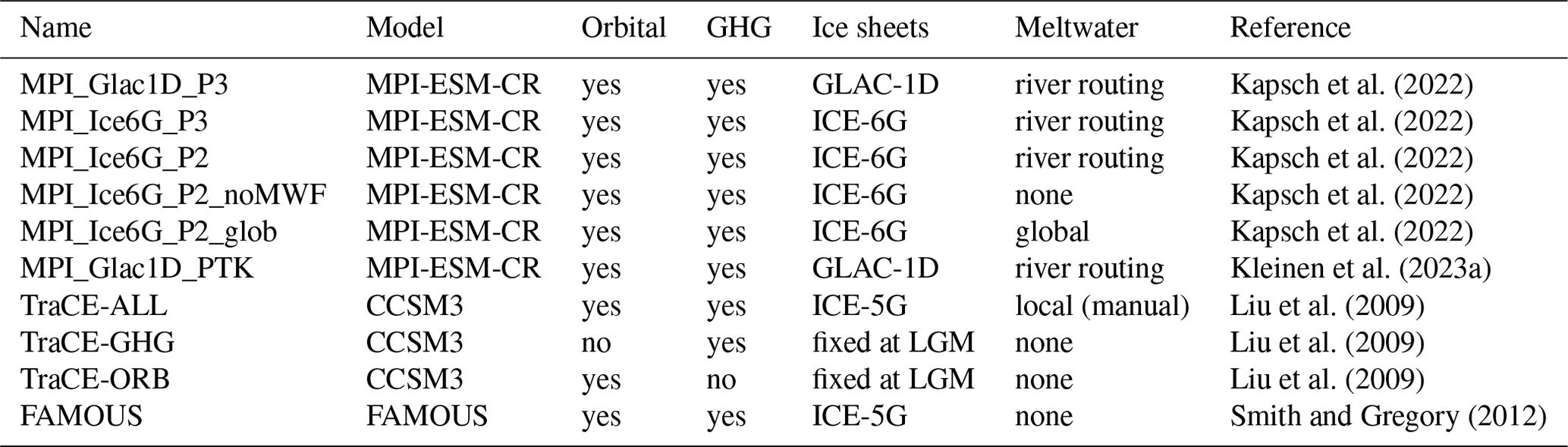
We use 10 previously published simulations from three climate models which all simulate the period 22 to 6 ka (Fig. 1, Table 1). Six simulations employ MPI-ESM-CR (Kapsch et al., 2022; Kleinen et al., 2023a, b). In these simulations, GHG concentrations and orbital parameters are updated transiently. Ice sheet topographies are changed according to the GLAC-1D or ICE-6G reconstructions (see Table 1). Meltwater from ice sheets is either transported into the ocean using dynamic river routing (Riddick et al., 2018), distributed uniformly over all grid cells, or removed from the system (see Table 1). MPI_Glac1D_PTK uses a parameter configuration that leads to a smaller LGM-to-Holocene temperature difference than in the other MPI-ESM simulations. Furthermore, atmospheric parameters in the “P3” simulations are slightly different from those in the “P2” simulations to correct a pre-industrial cold bias (Kapsch et al., 2022).

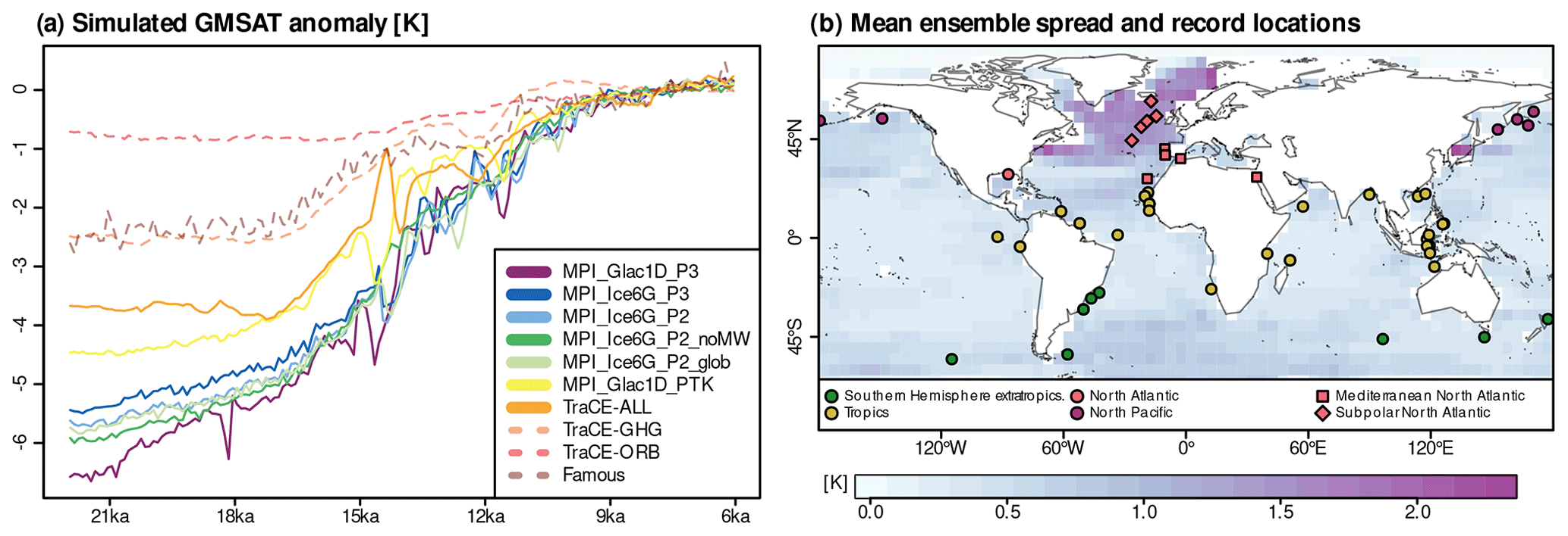
Figure 1 (a) GMSAT anomalies of the transient simulation ensemble members. Anomalies were computed with respect to the mean in the window 9 to 6 ka. (b) Locations of SST reconstruction records employed in the model–data comparison (dots) and simulation ensemble spread as measured by the standard deviation at each location and time step, averaged over all time steps (colors in the background). The colors of the dots indicate the regions considered in Sect. 4.2 and the shape of the dots in the North Atlantic mark the records used for the separation into Mediterranean and subpolar North Atlantic in Sect. 4.2 and Fig. 9. Ocean grid cells are selected based on the ICE-6G history (Peltier et al., 2015).

Kapsch et al. (2022)Kapsch et al. (2022)Kapsch et al. (2022)Kapsch et al. (2022)Kapsch et al. (2022)Kleinen et al. (2023a)Liu et al. (2009)Liu et al. (2009)Liu et al. (2009)Smith and Gregory (2012)

Table 1 Properties of the 10 transient simulations of the last deglaciation included in the simulation ensemble: the name used throughout the paper, the employed climate model, whether orbital and GHG forcings were varied transiently or fixed at LGM values, the employed ice sheet reconstructions, how meltwater fluxes were applied (local input through dynamical river routing, local input according to a manually defined scheme, distributed equally across all grid cells, or no meltwater input), and the main reference of the simulation.

We further include three CCSM3 simulations from the TraCE-21ka project (Liu et al., 2009). In TraCE-ALL, orbital parameters, GHG concentrations, ICE-5G ice sheet topographies, and manually prescribed meltwater fluxes are adapted transiently. In TraCE-GHG, all boundary conditions except for GHG concentrations are fixed at the 22 ka state of TraCE-ALL. Similarly, only orbital parameters are changed in TraCE-ORB. Finally, we use the ALL-5G simulation from the QUEST FAMOUS last glacial cycle ensemble (Smith and Gregory, 2012). Orbital parameters, GHG concentrations, and Northern Hemisphere ICE-5G ice sheet topographies are updated transiently. In contrast to the other simulations, the Antarctic ice sheet topography and land–sea mask are fixed to pre-industrial values, and the transient boundary conditions are applied with an acceleration factor of 10. No meltwater fluxes are applied in FAMOUS.

In the following, we denote the six MPI-ESM simulations and TraCE-ALL as the “main set of simulations” and TraCE-ORB, TraCE-GHG, and FAMOUS as “sensitivity experiments”. The latter three simulations either change only one boundary condition transiently or employ boundary conditions faster than they occurred in reality. Therefore, we do not expect them to cover all changes in the climate system with the same degree of realism as the other seven simulations. More information on the simulations is provided in the Supplement (Sect. S2).

The simulation ensemble has a large spread in the four components of the deglacial temperature evolution described in Sect. 1 (Fig. 1). In the main set of simulations, the deglacial GMSAT increase is between ∼ 4 K in TraCE-ALL and ∼ 6.5 K in MPI_Glac1D_P3. With ∼ 1 K in TraCE-ORB and ∼ 3 K in TRACE-GHG and FAMOUS, the deglacial warming is lower in the three sensitivity experiments. Deglacial warming starts later in TraCE-ALL than in the MPI-ESM simulations, and the warming trend is smoother in MPI-ESM than in TraCE-ALL. Two different aspects of meltwater injection appear to play an important role in the GMSAT histories of these runs: the method of application and the progression through time. Simulations without meltwater fluxes feature weak millennial-scale fluctuations (e.g., MPI_Ice6G_P2_noMWF), and simulations with locally applied meltwater fluxes (e.g., MPI_Ice6G_P2) generate stronger GMSAT fluctuations than the simulation with global injection (MPI_Ice6G_P2_glob). Differing meltwater histories lead to an abrupt warming at ∼ 14.5 ka in TraCE-ALL but cooling events in the MPI-ESM experiments with meltwater input.

2.2 Sea surface temperature reconstructions

We use temperature reconstructions from the PalMod 130k marine paleoclimate data synthesis v1.1.1 (Jonkers et al., 2023), which is a compilation of published proxy records derived from marine sediment cores. V1.1.1 is an update from Jonkers et al. (2020) with 252 published (near-)surface temperature time series covering various periods of the last glacial cycle. As described in Jonkers et al. (2020), age models are harmonized using the Bayesian age modeling algorithm BACON (Blaauw and Christen, 2011). For each sediment core, 1000 iterations of the age–depth model are saved in the database to quantify chronological uncertainties. The database combines temperature reconstructions from multiple proxies which are taken unchanged from the original publications. For some proxy records, reconstructions from different original publications are included in the database. We retain all records from the same sediment cores if they are based on different proxies. We average reconstructions originating from the same sediment core and proxy if all sample depths coincide. If the depths differ, we select the time series covering the longest period during the deglaciation. Reconstructions from the same proxy data but calibrated for different seasons are averaged to obtain pseudo-annual temperatures. More details on the preprocessing of the proxy records are provided in the Supplement (Sect. S3).

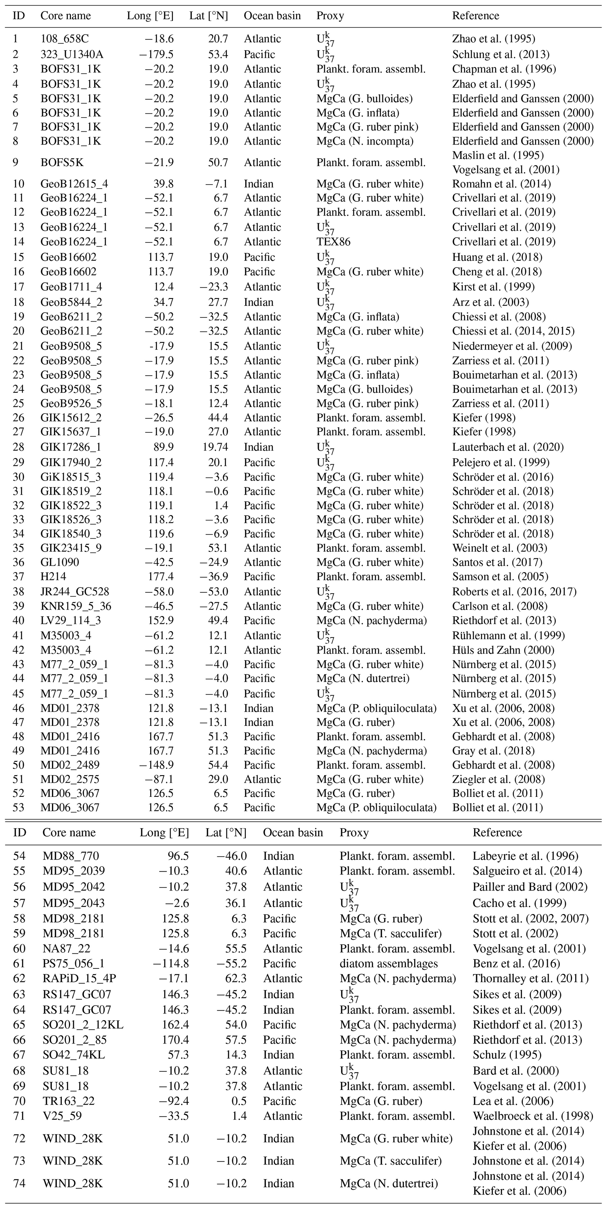
We select all (near-)surface temperature samples in the interval 22–6 ka from the database. Most of these records reflect surface or mixed-layer temperatures (Kucera et al., 2005; Rebotim et al., 2017; Tierney and Tingley, 2018). While the used sensors occupy a range of depths, we denote all samples as sea surface temperature (SST) reconstructions in the following. To compute robust statistics, we use only time series with at least 10 samples, which cover more than 8 kyr and have a mean temporal resolution of at least 1 kyr. 74 temperature records from 50 unique sediment cores satisfy these conditions (Fig. 1b, Table ). Most of them are located on continental margins with the biggest clusters located in the North Atlantic and the Indo-Pacific Warm Pool. A total of 38 temperature records are reconstructed from Mg $/$ Ca, 17 from U${}_{\mathrm{37}}^{\mathrm{k}}$, 17 from planktonic foraminifera assemblages, 1 from TEX₈₆, and 1 from diatom assemblages. Unlike some recent studies focusing on either assemblage-based temperature reconstructions (e.g., Paul et al., 2021) or geochemical proxies (e.g., Osman et al., 2021), we employ a multi-proxy approach using the calibrations proposed by the original authors for assemblages and geochemical proxies, respectively. We make this choice because the number of records in the database is too small to focus on specific proxy types, and proxy types tend to be regionally clustered, which makes a systematic assessment of differences between them unfeasible within our study design. For more discussion on the differences between proxy types, see Paul et al. (2021), and the references therein.

Zhao et al. (1995)Schlung et al. (2013)Chapman et al. (1996)Zhao et al. (1995)Elderfield and Ganssen (2000)Elderfield and Ganssen (2000)Elderfield and Ganssen (2000)Elderfield and Ganssen (2000)Maslin et al. (1995)Vogelsang et al. (2001)Romahn et al. (2014)Crivellari et al. (2019)Crivellari et al. (2019)Crivellari et al. (2019)Crivellari et al. (2019)Huang et al. (2018)Cheng et al. (2018)Kirst et al. (1999)Arz et al. (2003)Chiessi et al. (2008)Chiessi et al. (2014, 2015)Niedermeyer et al. (2009)Zarriess et al. (2011)Bouimetarhan et al. (2013)Bouimetarhan et al. (2013)Zarriess et al. (2011)Kiefer (1998)Kiefer (1998)Lauterbach et al. (2020)Pelejero et al. (1999)Schröder et al. (2016)Schröder et al. (2018)Schröder et al. (2018)Schröder et al. (2018)Schröder et al. (2018)Weinelt et al. (2003)Santos et al. (2017)Samson et al. (2005)Roberts et al. (2016, 2017)Carlson et al. (2008)Riethdorf et al. (2013)Rühlemann et al. (1999)Hüls and Zahn (2000)Nürnberg et al. (2015)Nürnberg et al. (2015)Nürnberg et al. (2015)Xu et al. (2006, 2008)Xu et al. (2006, 2008)Gebhardt et al. (2008)Gray et al. (2018)Gebhardt et al. (2008)Ziegler et al. (2008)Bolliet et al. (2011)Bolliet et al. (2011)Labeyrie et al. (1996)Salgueiro et al. (2014)Pailler and Bard (2002)Cacho et al. (1999)Stott et al. (2002, 2007)Stott et al. (2002)Vogelsang et al. (2001)Benz et al. (2016)Thornalley et al. (2011)Sikes et al. (2009)Sikes et al. (2009)Riethdorf et al. (2013)Riethdorf et al. (2013)Schulz (1995)Bard et al. (2000)Vogelsang et al. (2001)Lea et al. (2006)Waelbroeck et al. (1998)Johnstone et al. (2014)Kiefer et al. (2006)Johnstone et al. (2014)Johnstone et al. (2014)Kiefer et al. (2006)

Table 2 Information on the 74 proxy records selected for the deglacial model–data comparison.

3 Methods

This section first presents our model–data comparison algorithm (Sect. 3.1). The algorithm employs a simple PSM with two parameters that we estimate in Sect. 3.2. Section 3.3 describes the PPEs for assessing the reliability and robustness of our algorithm.

3.1 Model–data comparison algorithm

As visualized in Fig. 2, our model–data comparison algorithm consists of four main steps which we present in the following. An enhanced description of the algorithm with computational details is provided in the Supplement (Sect. S4).

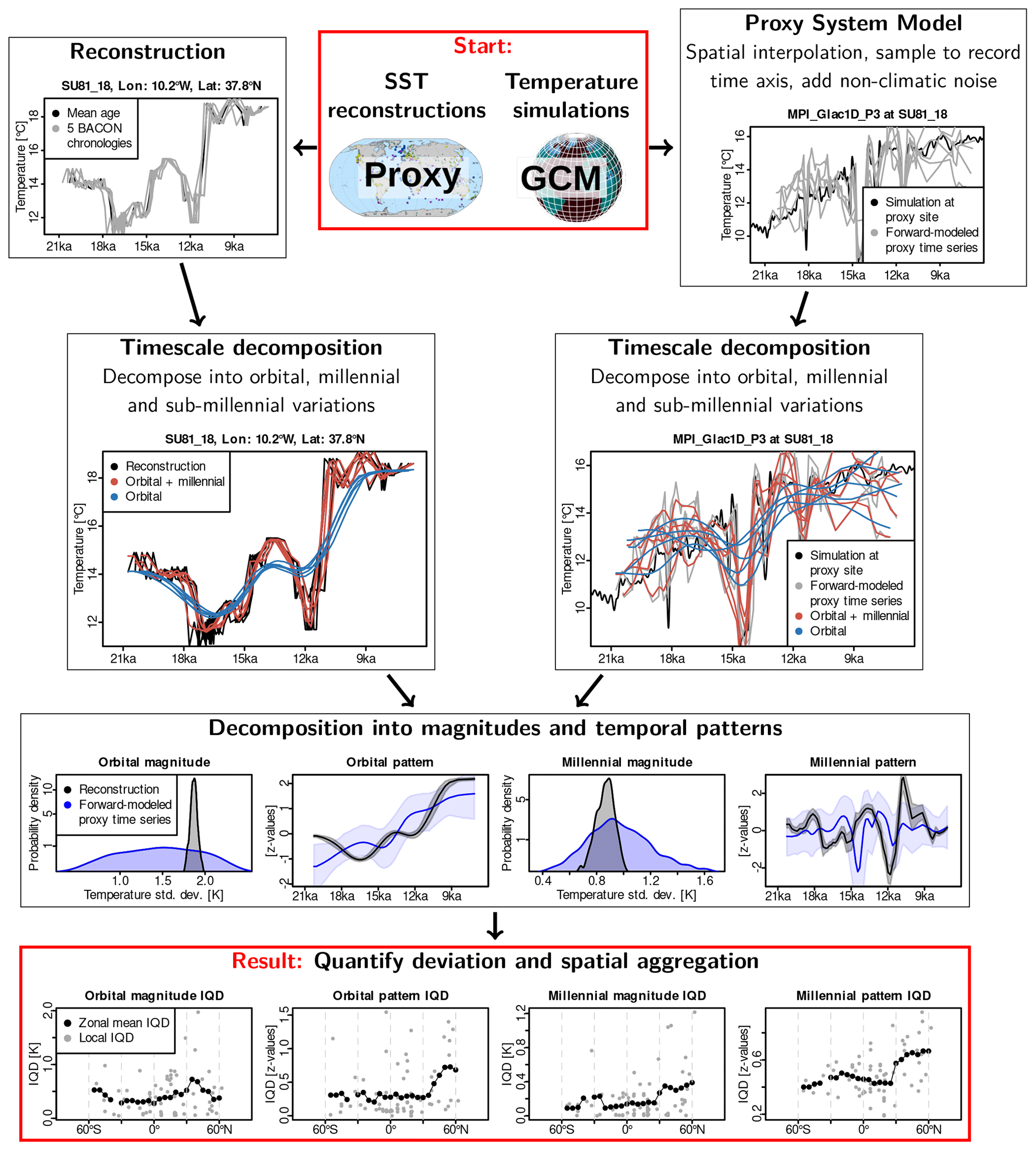
Figure 2 Flow chart describing the algorithm presented in this study (see Sect. 3 for details). We start at the top with two sets of data, reconstructed and simulated SSTs. Age uncertainties of the proxy records are quantified using multiple iterations from the age–depth model (top row, left). We apply a proxy system model (PSM) to the simulated SST fields to first obtain simulated time series interpolated to the proxy locations and then Monte Carlo realizations of forward-modeled proxy time series (top row, right). For each Monte Carlo realization, a timescale decomposition is performed to separate orbital- and millennial-scale variations using Gaussian smoothers (second row, left for reconstructions, right for forward-modeled proxy time series). Differences between the Monte Carlo realizations of reconstructions are due to chronological uncertainties, whereas differences in the Monte Carlo realizations of forward-modeled proxy time series result from the stochastic PSM. The orbital- and millennial-scale time series are decomposed into the magnitude and temporal pattern of the variations. This leads to probability distributions for reconstructions and forward-modeled proxy time series (third row). Finally, the integrated quadratic distance (IQD) between the probability distributions of reconstructions and forward-modeled proxy time series is computed for each of the four components (dots in the bottom row), and IQDs are averaged spatially. As an exemplary partition into regions, we show zonal mean IQDs in the bottom row for all latitudinal bands containing at least five proxy records (see Sect. 3.1 for a definition of the zonal mean averaging procedure).

3.1.1 Compute forward-modeled proxy time series from simulation output.

To compare simulations and reconstructions, we have to bridge the gaps between the two types of data in terms of spatio-temporal coverage and non-climatic influences on the proxy measurements. This is done in a forward approach, in which a PSM is applied to simulation output. The PSM output, which we call “forward-modeled proxy time series”, is compared to the measured proxies. We perform this comparison in temperature units instead of measured proxy units because it allows for averaging deviations from different proxies and no established forward calibrations exist for assemblage-based reconstructions. Our PSM takes simulated 3D (long × lat × time) mean annual SST fields (T_Sim) as input and modifies them to resemble a reconstructed SST record (T_FM, where FM stands for forward-modeled). The PSM consists of three steps: spatial interpolation to the proxy location (P_space), temporal downsampling to the proxy time axis (P_time), and a Gaussian additive noise process ε with a specified signal-to-noise ratio (SNR) and temporal autocorrelation structure. The noise process summarizes the effects of inherent uncertainties of the SST reconstructions (see Sect. 1) and uncertainties in the formulation of the PSM. Thus, the PSM is defined as follows:

$$\begin{array}{}\text{(1)}& T_{\mathrm{FM}}=P_{\mathrm{time}}\left(P_{\mathrm{space}}\left(T_{\mathrm{Sim}}\right)\right)+\mathit{\epsilon }.\end{array}$$

Accounting for reconstruction uncertainties, which is done in the temporal downsampling and additive noise components of the PSM, requires a probabilistic comparison framework. We implement such a framework using a Monte Carlo approach, which propagates uncertainties through the algorithm.

3.1.2 Decompose time series into magnitudes and temporal patterns of timescale-dependent variations.

We decompose each temperature time series into four components, orbital magnitude, orbital temporal pattern, millennial magnitude, and millennial temporal pattern, each of which is designed to assess one of the four questions posed in Sect. 1. For the timescale decomposition, we use Gaussian smoothers (Fig. 2, second row; see Figs. S2–S9 in the Supplement for further examples of timescale decompositions) as they are a robust method for the analysis of irregularly spaced time series in the time and frequency domain (Rehfeld et al., 2011). For each timescale, we define the magnitude of variations as the standard deviations of the filtered time series and the temporal pattern as the normalized, i.e., centered and standardized, time series (Fig. 2, third row).

Magnitude components quantify the strength of timescale-dependent variations, independent of their specific timing. Therefore, they are valuable for assessing the strength of the response to forcing, of spontaneous fluctuations, and of variations forced by time-uncertain boundary conditions. In contrast, temporal pattern components assess the direction, timing, and succession of timescale-dependent variations. They are particularly meaningful if variations are externally forced and if there are sufficiently tight constraints on the boundary condition reconstructions such that models can be expected to reproduce the timing of the observed pattern of variations. Since orbital- and millennial-scale variations are likely driven by different forcings and internal processes, we separate between deviations on these two timescales. We assess the deviations between forward-modeled proxy time series and proxy records for each component separately because computing a single score for the deviation between simulations and reconstructions is prone to conceal sources of discrepancies. For example, a simulation could reproduce the reconstructed spatio-temporal temperature pattern accurately but receive a poor score due to an underestimation of the LGM-to-Holocene temperature change.

3.1.3 Quantify deviations between reconstructions and forward-modeled proxy time series for individual proxy records.

The decompositions in step 2 result in probability distributions of forward-modeled proxy time series and the corresponding reconstructed SST records because we account for chronological uncertainties and include a noise process in the PSM. We quantify the deviations between these probability distributions with a distance function that takes into account the full, potentially multivariate probability distributions and not just summary statistics like the mean or standard deviation. We choose the integrated quadratic distance (IQD), which is a proper divergence function that has desirable mathematical properties for model selection as it penalizes overly confident or conservative uncertainty estimates compared to the unknown true uncertainties (Thorarinsdottir et al., 2013). Applying the distance function to the respective probability distributions results in a single number for the deviation between forward-modeled proxy time series and reconstructions for each of the four components in which we decompose the time series in step 2.

For two probability distributions ℙ and ℚ, the IQD takes positive values ($\mathrm{IQD}(\mathbb{P},\mathbb{Q})\ge \mathrm{0}$). It is only zero when ℙ and ℚ are equal ($\mathrm{IQD}(\mathbb{P},\mathbb{P})=\mathrm{0}$). Smaller IQD values imply a smaller deviation and thus a better agreement of forward-modeled proxy time series and reconstructions. In the absence of age and proxy uncertainties, the IQD reduces to the mean absolute difference between numbers (magnitudes) or time series (patterns). The IQD can be applied to quantities of arbitrary units. In our case, the units are temperature [K] for the comparison of magnitudes, and standard deviations [z] for patterns.

3.1.4 Average deviations in space.

Deviations between forward-modeled proxy time series and reconstructions can depend strongly on the unknown manifestation of non-climatic influences in the measured proxies and uncertainties in the PSM structure. Assuming that most non-climatic processes and PSM uncertainties are uncorrelated between proxy records, the influence of these processes can be reduced by spatially averaging deviations computed for individual proxy records. Computing averages in this last step instead of averaging temperature time series in the beginning avoids interpolating proxy records with irregular time axes to a common resolution. We analyze IQDs averaged on four spatial scales: locally, regionally (see color-coding of dots in Fig. 1b for the assignment of proxy records to the regions considered in this study), zonally, and globally. For local IQDs, we treat each proxy record individually, i.e., without averaging proxy records from the same core or nearby locations. Zonal IQDs are obtained by averaging over proxy records within overlapping bands of 20° width that move in 5° steps (Fig. 2, bottom row). We only consider latitudinal bands containing at least five proxy records to only incorporate spatial averages where we can assume that a substantial amount of non-climatic influences is averaged out.

3.2 Estimation of proxy system model parameters

The PSM described in Sect. 3.1 requires a SNR parameter quantifying the ratio between climatic and non-climatic variations and the specification of a temporal autocorrelation structure of the additive Gaussian noise process. Previous studies only estimated SNRs and autocorrelations for a subset of our proxy types (U${}_{\mathrm{37}}^{\mathrm{k}}$, Mg $/$ Ca) on sub-orbital timescales (Laepple and Huybers, 2014; Reschke et al., 2019). Therefore, we estimate the PSM parameters using the SST reconstruction database (see Sect. 2.2).

To obtain these estimates, we decompose the SST records into a similar structure as Eq. (1), i.e., the sum of a local mean SST signal P_space(T) and a realization of a Gaussian noise process ε, which aggregates all deviations from the local mean SST signal. The decomposition starts by constructing clusters of SST records centered around each of the 74 SST records selected from the database. The clusters contain the records within a radius of $l\in \mathit{\{}\mathrm{100},\mathrm{200},\mathrm{\dots },\mathrm{1000}\mathit{\}}$ km around the central record (see Fig. 3 for an example cluster with n=3 records centered around record SO201_2_12KL). For each cluster, we compute a local mean signal by averaging over the records in the cluster (red line in Fig. 3a). More specifically, we interpolate nearby records to a regular temporal resolution of 100 years, center the records, and average over the resulting time series. We use the mean age model of each record and not the age ensemble members since we account for chronological uncertainties at a different step of the PSM. Using the age ensembles instead of the mean ages strongly reduces the estimated SNR and likely biases it low (not shown). Note that we average records of different temporal resolutions, which tends to underestimate high-frequency contributions to ε. However, all records have at least a millennial resolution such that the relevant millennial and orbital timescales should be less affected by the interpolation and subsequent averaging.

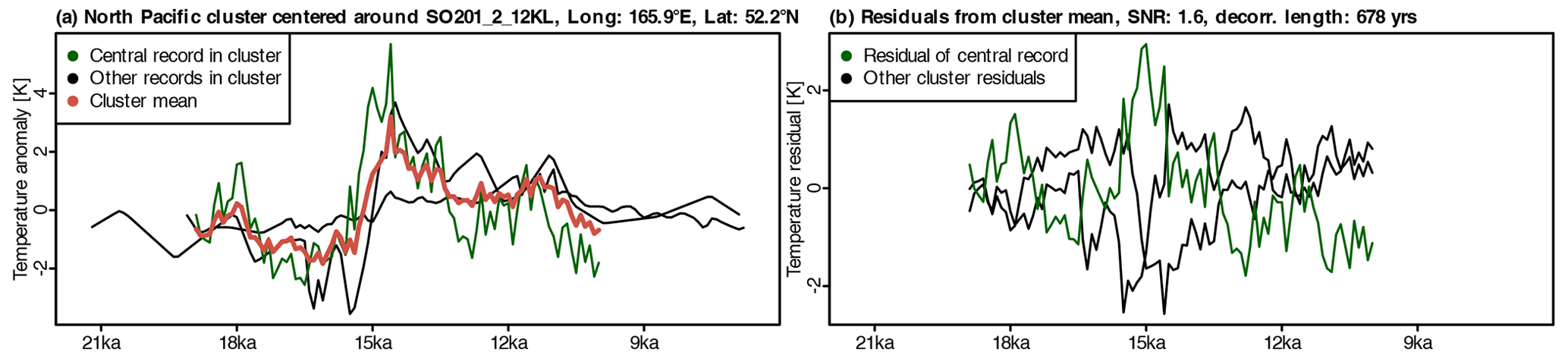
Figure 3 Visualization of the PSM parameter estimation as described in Sect. 3.2 for a cluster with 500 km radius and n=3 records in the North Pacific centered around the proxy record SO201_2_12KL. (a) All SST records in the cluster and the corresponding local mean SST reconstruction (red line) with the central record of the cluster in green. (b) Residual deviations from the local mean reconstruction with the central record in green. The SNR and decorrelation length for the central record (green) are given in the caption. SNRs are estimated by comparing the variance of the mean reconstruction (signal) against the variance of the residuals (noise). The decorrelation length of the noise process is estimated from the residual time series.

For the record in the center of the cluster, we compute the residual from the local mean signal (green line in Fig. 3b), which is treated as a realization of the Gaussian noise process (ε in Eq. 1). We compute the variance ratio between the local mean signal and the residual which provides an estimate of the SNR. Due to the short time series length, the structure of the temporal autocorrelation cannot be determined from the residuals. We choose to describe ε as an autoregressive process of order one (AR1) because it is determined by only two parameters and as a compromise between a white noise process without temporal autocorrelation and power law processes with long-range autocorrelations. This AR1 process is specified by the SNR and a decorrelation length, which we estimate from the residual. We iterate this process for all 74 records if the clusters around the respective records contain at least a specified number of records. We then take the medians of the SNRs and the decorrelation lengths in all clusters to reduce the noise in the parameter estimates, which results from the predominantly small cluster sizes (most clusters contain less than five records). As the estimates can be sensitive to the construction of the clusters, we apply this procedure for cluster radii of $l\in \mathit{\{}\mathrm{100},\mathrm{200},\mathrm{\dots },\mathrm{1000}\mathit{\}}$ km and for the minimum required number of records in a cluster of $n\in \mathit{\{}\mathrm{2},\mathrm{3}\mathit{\}}$.

The median SNR over all sensitivity experiments is 1.6±0.3 (1σ) and the median decorrelation length is 1289±212 years. When we decompose the SST variability of each proxy record into a signal and a noise component according to SNR = 1.6, the mean noise level across all records is 0.9±0.6 K. This estimate is consistent with an estimate of 0.6–1.3 K by Tierney et al. (2020) in a data assimilation framework characterizing LGM-to-Holocene anomalies. Our estimate is slightly higher than the SNR of 1.0 employed in the LGM climate field reconstruction by Paul et al. (2021).

3.3 Pseudo-proxy experiments

We use PPEs for the following three purposes: (i) to demonstrate the main features in the simulations that are captured by the model–data comparison algorithm; (ii) to diagnose how much model–data comparison results depend on limited temporal resolution, chronological uncertainties, and the magnitude and temporal autocorrelation structure of non-climatic noise; and (iii) to investigate how sensitive results are when noise magnitude and temporal autocorrelation structure in the PSM are different from their optimal values. Note that the difference between (ii) and (iii) is that (ii) is motivated by quantifiable limitations and uncertainties of reconstructions, while (iii) specifically targets the fact that the employed PSM is just an approximation of reality and its optimal parameters are unknown.

In PPEs, the underlying climate evolution is given by a reference simulation. The temperature time series of the reference simulation at each proxy location serves as the ground truth in the PPE. For each proxy record, the PSM from Sect. 3.1 is applied to the reference simulation to generate a single realization of forward-modeled proxy time series with a randomly selected iteration of the age–depth model and one realization of the non-climatic noise process. As this realization mimics the properties of the SST reconstructions, we call it a pseudo-proxy. We simulate pseudo-proxies at the locations and with the time axes and chronological uncertainties of the 74 selected proxy records from Sect. 2.2. Following this, the algorithm from Sect. 3.1 is employed to compute the deviations between N=100 realizations of forward-modeled proxy time series derived from each simulation and the pseudo-proxies.

For (i), we use an example PPE with a subset of simulations to illustrate how simulation characteristics such as parameter configurations and the implementation of boundary conditions influence their ranking by our algorithm. We use MPI_Glac1D_P3 as reference simulation and PSM parameters given by the estimates from Sect. 3.2 (SNR = 1.6, decorrelation length = 1289 years). For the PPE, we select simulations that differ from the reference simulations in boundary conditions (MPI_Ice6G_P2_noMWF, TraCE-ALL), parameter configuration (MPI_Glac1D_PTK), and employed climate model (TraCE-ALL). Additionally, two idealized modifications of MPI_Glac1D_P3, which are shifted in time by 2 kyr in either direction (MPI_Glac1D_P3-2k, MPI_Glac1D_P3+2k), show the effects of a timing mismatch in the deglacial temperature evolution on the model–data comparison results (Fig. 4a).

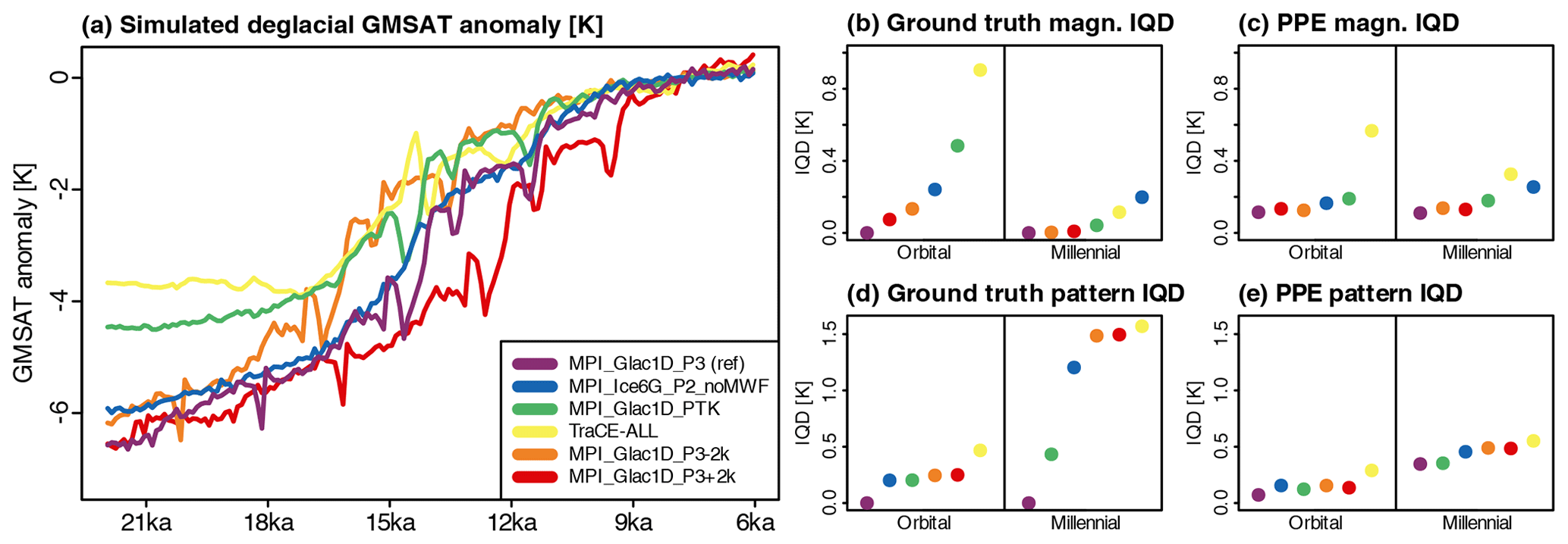
Figure 4 Visualization of the results for a PPE with SNR = 1.6, an AR1 noise process with a decorrelation length of 1289 years, and MPI_Glac1D_P3 as reference simulation. (a) GMSAT anomalies of the four simulations and the two time-shifted versions of MPI_Glac1D_P3 (anomalies with respect to the mean in the window 9 to 6 ka). Panels (b) and (d) show the ground-truth magnitude and pattern IQDs (see Sect. 3.3 for details). Panels (c) and (e) are the corresponding deviations between forward-modeled proxy time series and pseudo-proxies constructed from the reference simulation. Note that by definition the ground truth deviations in (b) and (d) of the reference simulation MPI_Glac1D_P3 from itself are zero.

For (ii) and (iii), we perform two sets of PPEs (Table 3). In the first set we assume that the noise magnitude and type in the PSM are known but we systematically vary the noise level of the records from very high (SNR $=\mathrm{1}/\mathrm{4}$) to very low (SNR = 16) and include PPEs without additive noise process (SNR = Inf). We further vary the noise type between white noise (no autocorrelation), an AR1 process with a decorrelation length of 1 kyr, and a self-similar process following a power law distribution with exponent one (red noise). Using all 10 transient simulations as reference simulations to avoid spurious results from selecting a specific reference simulation, we perform in total 240 PPEs (8 SNRs, 3 noise types, 10 reference simulations).

Table 3 Characteristics of the example PPE and the two sets of PPEs described in Sect. 3.3. For set 1, all combinations of reference simulations, pseudo-proxy SNRs, and pseudo-proxy noise types are employed with the same settings for pseudo-proxies and forward-modeled proxy time series. For set 2, the 12 combinations of reference simulations, pseudo-proxy SNRs, and pseudo-proxy noise types are employed with all combinations of forward-modeled proxy time series SNRs and noise types.

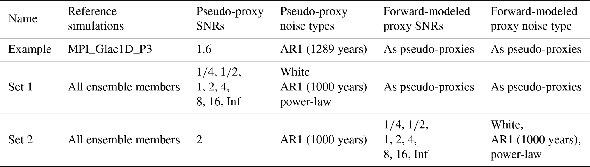
In the second set, the PSM structure used for generating the forward-modeled proxy time series employed in the model–data comparison algorithm deviates from the one selected to simulate the pseudo-proxies, thus imitating the case where the PSM structure is uncertain. For each of the 10 reference simulations, we draw a realization of pseudo-proxies with AR1 noise (SNR = 2, decorrelation length = 1 kyr). For each pseudo-proxy realization, we first apply the model–data comparison algorithm with varying noise levels in the PSM (SNR = $\mathrm{1}/\mathrm{4}$ to SNR = 16 and SNR = Inf) but the same autocorrelation structure as in the construction of the pseudo-proxies. Following this we apply the model–data algorithm with varying autocorrelation structure (white, AR1, and power-law noise) but the same noise level as in the construction of the pseudo-proxies.

Whether a certain IQD corresponds to an acceptable agreement between a simulation and a reconstruction is a subjective choice. Moreover, because the IQD uses the probability distribution of the forward-modeled proxy time series, its absolute value depends on the specification of the PSM. For example, a higher noise level results in a larger spread of the forward-modeled proxy time series created from the same simulation, such that the IQD for a high noise level will differ from the IQD for a low noise level, even if the simulated and reconstructed SST time series are the same. Therefore, we focus on the ability of the algorithm to reliably discriminate between simulations, i.e., determining whether simulation A is closer to reality than simulation B. In PPEs, we can compute the “ground truth deviation” between a simulation and the reference climate history that was used to construct the pseudo-proxies. We choose the mean absolute deviation from the reference simulation at the locations of the proxy records as ground truth deviation because the IQD reduces to the mean absolute difference in the absence of uncertainties. We then compute a reference ranking by sorting the simulations according to their ground truth deviations. Similarly, we can rank the simulations according to the IQDs between the forward-modeled proxy time series and the pseudo-proxies, which is the ranking that would be obtained in a real-world model–data comparison situation in which only the pseudo-proxies are known but not the underlying reference climate history. We call this the pseudo-proxy ranking.

Finally, we compare the reference ranking with the pseudo-proxy ranking. If the model–data comparison algorithm discriminated perfectly between simulations, the reference ranking and pseudo-proxy ranking would be identical. However, due to reconstruction uncertainties and limitations, this will not always be the case. To quantify the similarity of the two rankings, we introduce a measure called the “fraction of pairwise reversed rankings” (FPRR). This measure is based on pairwise comparisons of the rankings of simulations: if simulation A ranks higher than simulation B in the reference ranking but ranks lower in the pseudo-proxy ranking, we say that the ranking of the two simulations is reversed in the pseudo-proxy ranking, i.e., the two simulations are erroneously ranked by the model–data comparison algorithm. We assign 1 to the pairwise comparison if the ranking is reversed and 0 if it is not reversed. We compare the rankings for all pairs of simulations and define the FPRR as the mean of all pairwise comparisons. The FPRR is 0 when the pseudo-proxy and reference rankings are equal and is 1 if the two rankings are exactly reversed. The expected value for a random ranking of simulations is 0.5, which means that an FPRR below 0.5 indicates a better-than-random ranking. We focus on two aspects of the simulations' rankings: (i) the reliability of rankings, i.e., the expected probability of erroneously ranking simulations which we define as the median IQD in a set of PPEs with the same PSM parameters, and (ii) the robustness of rankings, i.e., how much the probability of an erroneous ranking depends on the reference climate history and the realization of non-climatic processes in the pseudo-proxies. Robustness is quantified by the spread of the IQD in a set of PPEs with the same PSM parameters and can be interpreted as a measure for the predictability of the reliability of model–data comparison results.

4 Results

We start this section with an example PPE that demonstrates the characteristics of the model–data comparison algorithm. We then use the PPE framework to systematically assess the dependency of model–data comparison results on uncertainties and limitations of SST reconstructions. Finally, we demonstrate our algorithm in a real-world setting by quantifying the deviations between deglacial simulations and SST reconstructions.

4.1 Pseudo-proxy experiments

4.1.1 Exemplifying pseudo-proxy experiment

As described in Sect. 3.3, we use an example PPE with MPI_Glac1D_P3 as reference simulation to demonstrate how a simulation's characteristics influence their ranking by our algorithm. The globally averaged ground truth deviations, i.e., IQDs between simulations and the reference simulation at the proxy locations with a regular temporal resolution, no chronological uncertainties, and no non-climatic noise are shown in Fig. 4b and d, and the IQDs from the comparison between forward-modeled proxy time series and pseudo-proxies are shown in Fig. 4c and e. For all four components of the deglacial temperature evolution (orbital magnitudes, millennial magnitudes, orbital patterns, and millennial patterns), the spread between IQDs corresponding to different simulations are smaller in the PPE (Fig. 4c, e) than in the ground truth deviations (Fig. 4b, d). This shows that in the presence of uncertainties, the forward-modeled proxy time series constructed from different simulations are harder to distinguish than the simulations in the uncertainty-free ground truth. However, the pseudo-proxy ranking mostly preserves the reference ranking (see Sect. 3.3 for a definition), which demonstrates the ability of the algorithm to still discriminate correctly between simulations in the presence of reconstruction limitations and uncertainties.

Comparing the IQDs with simulated global mean temperatures (Fig. 4a), we see that the orbital magnitude IQD rankings follow the differences in the magnitude of deglacial warming compared to the reference simulation. Meltwater fluxes have a strong influence on millennial magnitude rankings. MPI_Ice6G_P2_noMWF, in which no meltwater flux is applied, deviates substantially from the reference simulation. The varying spatial structure of millennial magnitudes due to the different meltwater history between TraCE-ALL and MPI_Glac1D_P3 seems to be exaggerated in the PPE. This leads to TraCE-ALL having a higher millennial magnitude IQD than MPI_Ice6G_P2_noMWF in the PPE but not in the ground truth.

The orbital pattern IQDs do not vary strongly between the MPI-ESM simulations, which all feature similar warming trends. In contrast, deglacial warming starts later and is more abrupt in TraCE-ALL, which results in a higher orbital pattern IQD. The difference in the meltwater histories is reflected in the millennial pattern component: MPI_Glac1D_P3 and MPI_Glac1D_PTK feature smaller IQDs than MPI_Ice6G_P2_noMWF, which does not exhibit pronounced millennial-scale fluctuations. The millennial pattern IQD is highest in TraCE-ALL, where a strong fluctuation around 14.5 ka is of opposite sign to MPI_Glac1D_P3.

In the reference rankings, as well as the PPE, the time-shifted versions of MPI_Glac1D_P3 are very similar to the reference simulation in the magnitude components (Fig. 4b, c). This is because the magnitude of orbital and millennial variations changes little under time shifts. In contrast, time-shifted versions deviate substantially from the reference simulation in the temporal patterns (Fig. 4d, e) because the timing of the start and end of the deglacial warming, as well as the millennial-scale fluctuations, differs from the reference simulation. This shows that the magnitude IQDs are insensitive to differences in the timing of events, whereas timing differences appear pronounced in the pattern IQDs.

4.1.2 Reliability and robustness of simulation rankings

We analyze the first set of 240 PPEs (see Sect. 3.3, set 1 in Table 3) by aggregating them according to the employed noise level and compare the respective FPRRs for three averaging scales: globally, zonally, and locally (Fig. 5). For all averaging scales, FPRRs increase for lower SNRs, i.e., pseudo-proxy rankings deviate more from the reference ranking for higher noise levels. However, even for the highest considered noise levels, the FPRRs are rarely above 0.5. Thus, there is almost always enough information of the underlying signal preserved to obtain a better than random ranking. There is no threshold behavior, but a steady FPRR increase for higher noise levels. This increase is expected since higher non-climatic noise levels make it harder to distinguish simulations.

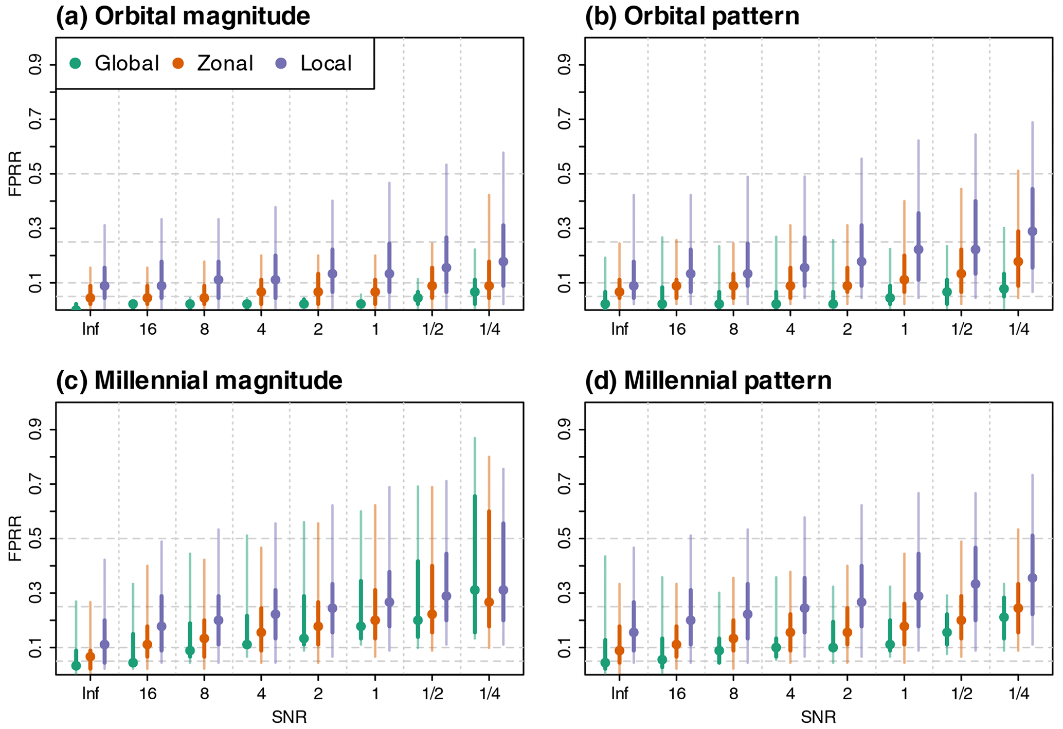
Figure 5 Fraction of pairwise reversed rankings (FPRR; see Sect. 3.3 for a definition) of simulations for globally averaged IQDs, zonally averaged IQDs, and IQDs of individual pseudo-proxy records. Shown are FPRRs for (a) orbital-scale magnitudes, (b) millennial-scale magnitudes, (c) orbital-scale temporal patterns, and (d) millennial-scale temporal patterns. Dots depict the medians across all PPEs with a given SNR (n=30 for each SNR). Bars show the spread across PPEs. Darker colors depict the 25th to 75th percentiles, whereas lighter colors depict the 5th to 95th percentiles. SNR = Inf corresponds to PPEs without additive noise process. Dashed horizontal lines indicate FPRRs of 0.05, 0.1, 0.25, and 0.5. FPRRs above 0.5 are worse than expected for a randomized ranking.

On average, rankings of orbital magnitudes differ least from the reference rankings, followed by orbital patterns, and millennial patterns. Millennial magnitude rankings are the least reliable under non-climatic noise. More reliable orbital than millennial rankings are expected because temperature variations are larger on orbital than millennial timescales whereas the noise level does not increase by the same rate on longer timescales. Median FPRRs mostly increase for decreasing spatial averaging scales, i.e., the reliability of rankings decreases from globally to locally averaged IQDs. The spread of FPRRs over the PPEs with the same noise level tends to increase with higher noise level and smaller spatial averaging scale, too. Thus, model–data comparison results are not just less reliable but also less robust for higher noise levels and smaller averaging scales (see also Sect. 3.3). For our SNR estimates from Sect. 3.2, the PPE results suggest below 10 % expected erroneous simulation rankings for orbital magnitudes and patterns and 10 %–20 % for millennial patterns and magnitudes.

In reality, the magnitude and temporal structure of non-climatic processes is uncertain. Therefore, we test how robust model–data comparison results are when either the noise level or the temporal autocorrelation structure in the forward-modeled proxy time series differs from the values selected to construct the pseudo-proxies (see set 2 in Table 3). Figure S10 in the Supplement shows the FPRR for overestimated or underestimated SNRs and for overestimated (power-law) or underestimated (white noise) temporal persistence of non-climatic processes. We find small influences from moderately (factor 2 to 4) overestimating or underestimating the noise level. Substantial differences from the results for the true noise level only occur for strong deviations (larger than factor 4) from the true level or when non-climatic processes are neglected entirely (SNR = Inf), especially for millennial magnitudes. For the latter, the reliability tends to decrease when the noise level is overestimated, whereas the robustness decreases when the noise level is underestimated. Neglecting non-climatic noise entirely for millennial magnitudes reduces the reliability more for global averages than on smaller spatial scales (see also Sect. 5.1). For all averaging scales and all four components, the effects of misspecified temporal autocorrelation structures are negligible. This supports the decision to choose an AR1 process in Sect. 3.2 instead of trying to estimate the structure of the temporal autocorrelation function.

4.2 Comparison of simulations against SST reconstructions

Next, we quantify the deviations between forward-modeled proxy time series derived from the 10 deglacial simulations (Sect. 2.1) and the 74 selected SST records (Sect. 2.2). We employ a PSM with an AR1 non-climatic noise process and vary the SNR between 1.1 and 2.2 and the decorrelation length between 865 and 1712 years (Sect. 3.2). We study globally and regionally averaged IQDs for the Southern Hemisphere extratropics (n= 10 proxy records), the tropics (n= 44), the extratropical North Atlantic (n= 13), and the extratropical North Pacific (n= 7) (Fig. 1). We select these regions based on detected inter-regional dissimilarities of the deglacial temperature evolution in an initial visual inspection of reconstructions and simulations. The averaged temporal evolution of the reconstructed temperatures and forward-modeled proxy time series at the proxy record locations is depicted for each of the four disjunct regions in Fig. 6. All regions contain more than five records and thus we expect the results to benefit from the spatial averaging effect found in the PPEs. Figure 7 shows the IQDs for all four components of the deglacial temperature evolution, simulations, and regions. An alternative visualization of the deviations, which combines magnitude and pattern deviations for a given timescale, is provided in the Supplement (Figs. S11, S12). In the next two subsections, we assess orbital- and millennial-scale variations of our main set of simulations. Finally, we analyze the model–proxy agreement of the three sensitivity experiments.

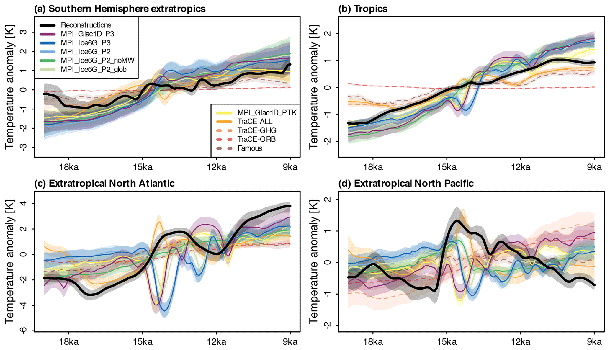
Figure 6 Regionally stacked SST variations for records in (a) the Southern Hemisphere extratropics (n=10 proxy records), (b) the tropics (n=44), (c) the extratropical North Atlantic (n=13), and (d) the extratropical North Pacific (n=7). Black lines denote the stacked reconstructions, whereas colored lines depict the stacked forward-modeled proxy time series derived from the 10 transient simulations. Shaded areas show uncertainties from chronologies and the PSM. Note that the stacks are not used in the model–data comparison algorithm but provide a visual impression of the reconstructed and simulated regional temporal evolution. The methodology to construct the stacks is described in the Supplement (Sect. S5).

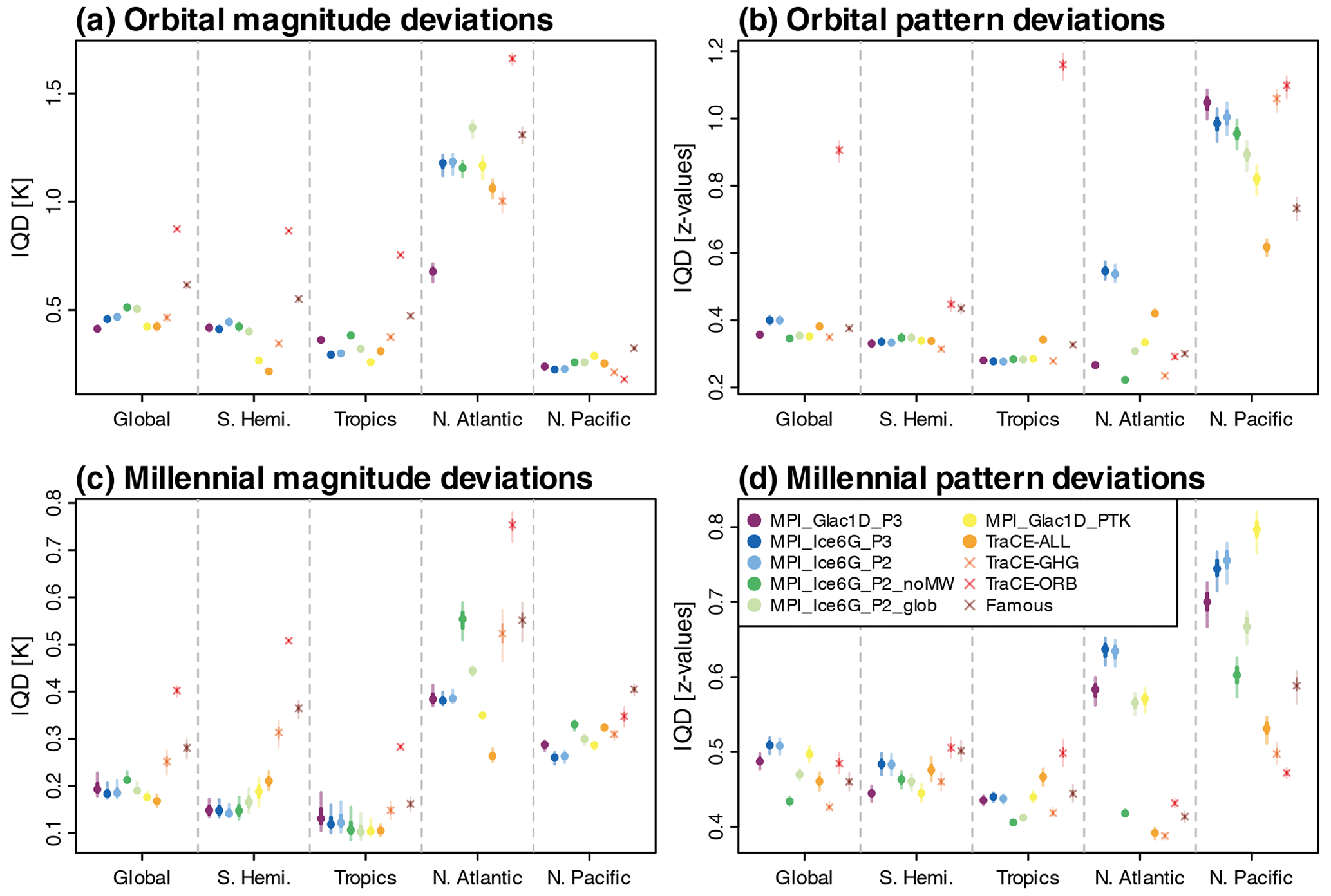
Figure 7 Global and regional mean IQDs of the 10 transient deglacial simulations from the 74 SST reconstruction records. Colored dots show median IQDs for (a) orbital magnitudes, (b) millennial magnitudes, (c) orbital temporal patterns, and (d) millennial temporal patterns. Darker colors depict the 25th to 75th percentiles resulting from varying the uncertain PSM parameters, whereas lighter colors depict the full range of uncertainties from varying the PSM parameters as described in Sect. 4.2. Note that the ranges of the y axes are different between the panels.

4.2.1 Orbital-scale variations

For orbital magnitudes, MPI_Glac1D_P3, MPI_Glac1D_PTK, and TraCE-ALL feature the smallest deviations between forward-modeled proxy time series and reconstructions in the global average (Fig. 7a). Among these three simulations, MPI_Glac1D_PTK and TraCE-ALL warm by ∼ 4 K during the deglaciation (see Fig. 1) and deviate less from the reconstructions than other simulations in the Southern Hemisphere and tropics. Meanwhile, MPI_Glac1D_P3 has the strongest deglacial warming among the simulations and deviates significantly less from the reconstruction in the North Atlantic than all other simulations. In the global average, these regionally varying agreements compensate each other, which shows that global mean temperature alone is insufficient to explain the rankings. In the tropics and Southern Hemisphere, forward-modeled proxy time series with median orbital magnitudes around 1 K tend to deviate least from the reconstructions (Figs. 7a, 8a). In the North Atlantic, no simulation matches the high orbital magnitudes of the reconstructions (Fig. 8a). Here, the simulation with the highest magnitude (MPI_Glac1D_P3) features the lowest IQDs. In the North Pacific, orbital magnitudes are much smaller than in the North Atlantic in reconstructions and all simulations, and IQDs are relatively similar for all simulations.

Figure 8 Mean absolute magnitudes of timescale-dependent variations of SST reconstructions (black) and forward-modeled proxy time series with the median PSM parameter estimates from Sect. 3.2 (color-coded). Depicted are globally and regionally averaged magnitudes of (a) orbital-scale and (b) millennial-scale variations. Points denote median magnitudes within a region. Darker color bars depict the 25th to 75th percentiles across all records within the respective region, whereas lighter colors depict the 5th and 95th percentile.

Turning to orbital patterns, the globally averaged IQD differences between simulations are relatively small (Fig. 7b). In the North Atlantic, two distinct regional clusters appear in the reconstructions (Fig. 9a, c): along the Iberian Margin and in the Mediterranean Sea (denoted Mediterranean North Atlantic; see Fig. 1b), the lowest SSTs occur during Heinrich Stadial 1 (∼ 17 ka), followed by two strong warming phases, which are interrupted by a warming hiatus during the Younger Dryas (∼ 12 ka). Meanwhile, warming is more monotonic in the subpolar North Atlantic (see Fig. 1b for a definition of the region). In contrast to the reconstructions, the orbital patterns are very similar between those two subregions of the North Atlantic in all of the simulations (Fig. 9a, c). Due to the differences between Subpolar and Mediterranean North Atlantic in the reconstructions, the lowest orbital pattern IQDs in the North Atlantic occur in MPI_Ice6G_P2_noMW and MPI_Glac1D_P3, which feature a smoother orbital pattern with weaker interruptions of the warming trend than other simulations. Among all examined regions, the highest orbital pattern IQDs occur in the North Pacific, where inter-model differences in orbital patterns are also the largest (Fig. 9e). Here, TraCE-ALL has the lowest IQD as it is the only simulation that somewhat resembles the pattern in the reconstructions with a temperature increase until ∼ 14 ka and subsequent cooling into the Holocene.

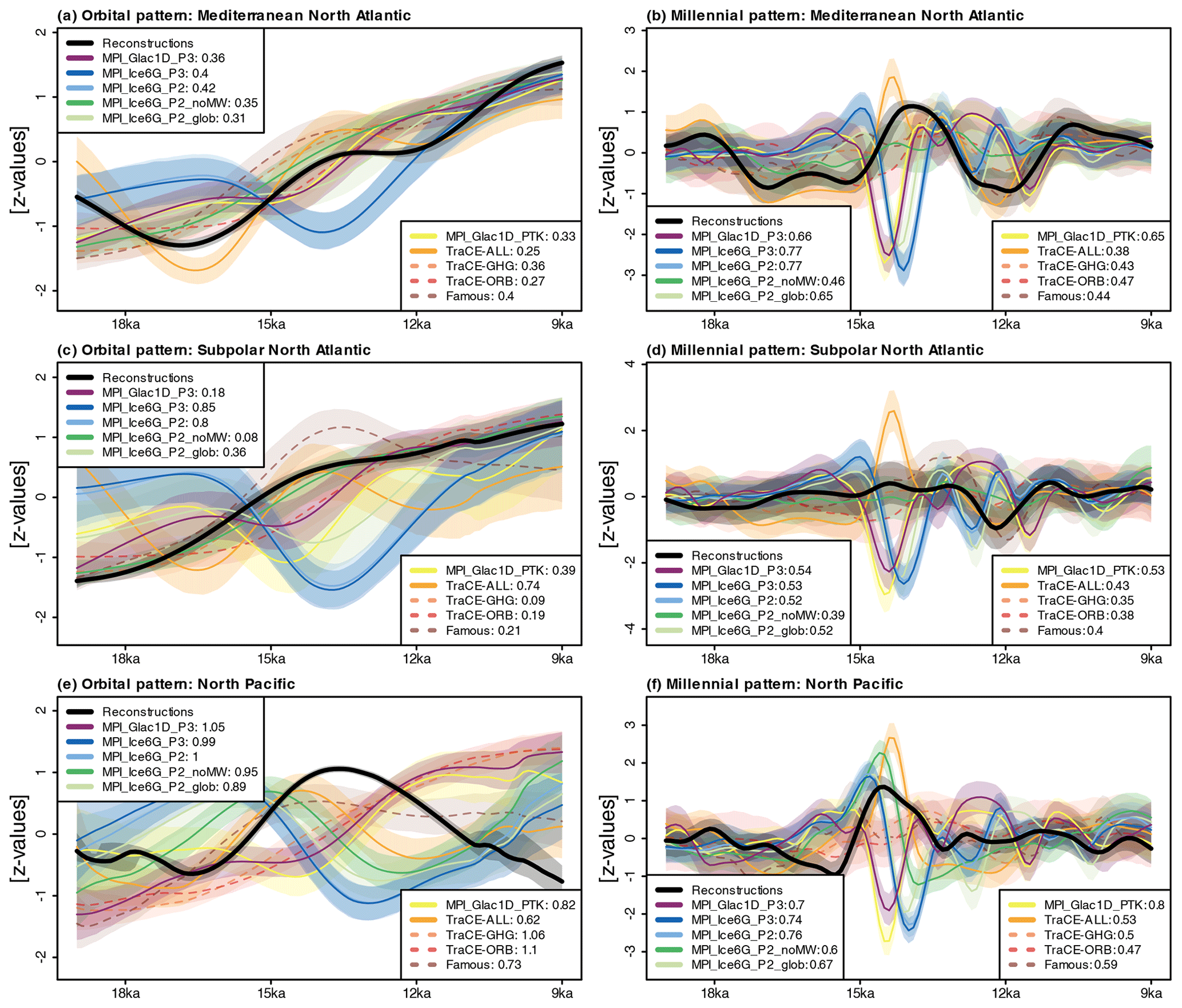
Figure 9 Regionally stacked temporal patterns of orbital-scale (a, c, e) and millennial-scale (b, d, f) variations for records in (a, b) the Mediterranean North Atlantic, (c, d) the Subpolar North Atlantic, and (e, f) the North Pacific (see Fig. 1 for the definition of the regions). Black lines denote the stacked reconstructions, whereas colored lines depict the stacked forward-modeled proxy time series derived from the 10 transient simulations. Shaded areas show uncertainties from chronologies and the PSM. The numbers in the legends next to each simulation are the averaged IQDs over all records in the respective regions. Note that the stacks are not used in the model–data comparison algorithm, but just facilitate the interpretation of the IQDs. The methodology to construct the stacks is described in the Supplement (Sect. S5).

4.2.2 Millennial-scale variations

Millennial magnitude IQDs exhibit small differences between the simulations containing meltwater-induced abrupt events when averaged globally as well as in the Southern Hemisphere extratropics and in the Tropics (Fig. 7c). The highest millennial magnitudes in reconstructions and simulations occur in the North Atlantic (Fig. 8b). Here, two simulations with medium millennial magnitudes, TraCE-ALL and MPI_Glac1D_PTK, have the smallest IQDs, whereas the largest deviations from the reconstructions occur for the simulation without meltwater input, MPI_Ice6G_P2_noMWF. Compared to the North Atlantic, millennial-scale variations are weaker in the North Pacific in reconstructions and simulations and IQDs are more similar between simulations.

Turning to millennial patterns, MPI_Ice6G_P2_noMWF, a simulation without distinct millennial-scale variations, features the lowest globally averaged IQD (Fig. 7d). This is because no single simulation with distinct millennial-scale variations reproduces the reconstructed millennial patterns effectively in all regions. The agreement between simulations and reconstructions even differs within the North Atlantic and between North Atlantic and North Pacific (Fig. 9). Here, the meltwater fluxes extracted from the ice sheet reconstructions through dynamic river routing in the MPI-ESM simulations lead to abrupt millennial-scale temperature variations that do not align with the reconstructions. TraCE-ALL matches the millennial-scale variability pattern in the Mediterranean North Atlantic and therefore features the smallest IQDs in this area (Fig. 9b). However, it deviates strongly from the reconstructions in the Subpolar North Atlantic (Fig. 9d) and North Pacific (Fig. 9f).

4.2.3 Comparison of sensitivity experiments

Finally, we assess the model–proxy agreement of the three sensitivity experiment simulations, TraCE-GHG, TraCE-ORB, and FAMOUS. TraCE-GHG forward-modeled proxy time series have mostly comparable IQDs to the main set of simulations (Fig. 7). Only for millennial magnitudes, the TraCE-GHG IQDs are substantially higher than for the main set of simulations, in particular in the Southern Hemisphere. In the North Atlantic, all simulations with freshwater input have lower millennial magnitude IQDs than TraCE-GHG. In the global average, TraCE-ORB has the highest IQDs for orbital magnitudes, orbital patterns, and millennial magnitudes (Fig. 7). This is the result of lower orbital and millennial magnitudes than the other simulations (Fig. 8) and the absence of a deglacial warming trend in the Southern Hemisphere (Fig.  6). TraCE-ORB does not deviate substantially more from the reconstructions than the other simulations only for millennial pattern IQDs. FAMOUS features higher magnitude IQDs than the main set of simulations in the global average and in most regions (Fig. 7). For the pattern components, FAMOUS IQDs are in the range of the main set of simulations in the global average and in all regions other than the Southern Hemisphere, where it has higher IQDs for orbital and millennial patterns.

5 Discussion

Our study is a first step towards quantitative spatio-temporal model–data comparison for transient simulations of past climate transitions, as demonstrated here for the last deglaciation. In this section, we explore reasons for the PPE results and their implications. We then discuss the agreement between transient simulations of the last deglaciation and SST reconstructions, provide ideas for testing potential reasons for disagreements, and suggest improvements for future applications.

5.1 Reliability and robustness of the model–data comparison algorithm

The systematic PPEs show that the reliability and robustness of simulation rankings decrease with increasing noise levels. This result is not surprising as higher noise levels make it harder to identify the underlying temperature signal. The effect can be reduced by spatially averaging results from multiple records. As we assume the non-climatic noise to be independent between records, averaging over IQDs from multiple records reduces the influence of the noise and thus effectively enhances the SNR. If modulations of the temperature signal were not independent between records in reality, the improvement from spatial averaging would be weakened.

Rankings for orbital-scale variations are more reliable and robust than for millennial-scale variations due to comparably smaller distortion by non-climatic noise. That orbital magnitude rankings tend to be more reliable and robust than orbital pattern rankings could be due to relatively subtle differences between simulations in the timing and shape of the deglacial warming trend compared to easier to identify differences in the magnitude of deglacial warming. On the other hand, we attribute more reliable and robust millennial pattern than magnitude rankings to the differing effects of non-climatic noise on these two components. Millennial patterns of simulations are often still distinguishable based on their most pronounced fluctuations that are comparatively less distorted by non-climatic noise. Meanwhile, non-climatic noise enhances the magnitude of reconstructed millennial-scale variations (in our PSM proportional to the variability of the simulation at a given location) and thus has a systematic effect on millennial magnitudes, which can further diminish the reliability of rankings.

If the assumed noise level in the model–data comparison is not strongly overestimated or underestimated (factor 4 and more), results remain reliable. Using explicitly conservative SNR values is not safeguarding from erroneous rankings as strongly overestimating noise levels reduces the reliability, whereas strongly underestimating noise levels reduces the robustness of rankings. Incorrect specifications of the temporal autocorrelation structure of non-climatic processes have a negligible effect in our PPEs. This rather unexpected result might be due to the relatively short time period of investigation (16 kyr) compared to the timescales we study. This hypothesis could be tested in future work by repeating the experiments for longer periods. Entirely neglecting existing non-climatic processes leads to less robust and reliable rankings for millennial-scale variations. On the one hand, this can be explained by non-climatic variations in reconstructions being interpreted as climate signals, such that rankings depend more on the unknown realization of non-climatic processes. On the other hand, underestimating millennial-scale variations by neglecting variability-enhancing processes can systematically distort millennial magnitude rankings. This effect is strongest for global averages.

Taken together, the PPE results suggest that the reliability and robustness of model–data comparison results can be improved the most by increasing the SNR. In contrast, reducing the uncertainty of SNR estimates or improving the specification of the temporal autocorrelation structures will barely improve rankings. A doubling of the SNR typically reduces erroneous rankings by 1–3 percentage points. Thus, incremental improvements, for example through process-based modeling of modulations of the recorded climate signal, will only have a small effect on the reliability of rankings. PPEs without non-climatic noise typically still have 5 %–10 % erroneous rankings for regionally averaged IQDs. This percentage could be reduced by more precise chronologies and higher temporal resolutions of records. Comparing global, zonal, and local estimates suggests that significantly improved reliability can also be achieved by increasing the number of proxy records and thus averaging over more records in regional averages, as long as non-climatic contributions are not strongly correlated between records.

5.2 Agreement of SST reconstructions and deglacial simulations

The diversity of the simulations in terms of employed climate models and experiment protocols makes interpreting the results challenging. Comparing TraCE-ALL and the six MPI-ESM simulations, we find that none of the simulations ranks among the simulations with the smallest deviation from the reconstructions across all four components and considered regions. We confirm this visual impression from Fig. 7 by computing rank histograms among the main set of simulations. Rankings are computed for each proxy record and each of the four components. Averaged over all records and components, the ranks of the simulations are between 3.8 (for MPI_Glac1D_PTK and MPI_Ice6G_P2_glob) and 4.2 (for MPI_Glac1D_P3) with TraCE-ALL at an average rank of 4.0 (Fig. S13 in the Supplement). However, the ranks of TraCE-ALL concentrate strongly at 1 (highest agreement) and 7 (lowest agreement). In contrast, the rank histograms of the MPI-ESM simulations are flatter; i.e., they feature more similar occurrence rates across ranks. Thus, TraCE-ALL IQDs are more often outside than inside the range of the MPI-ESM simulations, even though it does not feature a consistently higher or lower rank. The concentration of TraCE-ALL at extreme ranks tends to hold for all four components (Figs. S14–S17). At the moment, we cannot attribute the difference in the rank score histograms to differences between either the used climate models or the employed experiment protocols. This is due to the differences in the experiment protocol between TraCE-ALL and the MPI-ESM simulations, particularly regarding the location, timing, and magnitude of freshwater injections. Nevertheless, the flatter rank histograms of the MPI-ESM simulations, despite substantial experiment protocol and parameter configuration differences among them, hint at a substantial influence from climate model differences.

Examples of regionally varying mismatches between simulations, which compensate in global averages, are found for all four components of the deglacial temperature evolution (see Sect. 4.2). These compensations occur because simulations with higher variability than others have higher variability in almost all regions (Fig. 8). Additionally, simulations tend to have similar temporal patterns at least within each hemisphere (Figs. 6, 9). In contrast, the reconstructed variability magnitudes are the most similar to the simulations with the highest variability in some regions, but closer to those with low variability in others. Similarly, the reconstructed variability patterns vary more between and within ocean basins than in the simulations. Therefore, we attribute the absence of a simulation with consistently high agreement relative to the others to more regionally confined variability magnitudes and patterns in reconstructions than in simulations. In other words, the reconstructed spatial variability of the deglacial temperature evolution is higher than in all considered simulations. For the North Atlantic, the differences in the reconstructed deglacial temperature evolution between the Mediterranean and the Subpolar North Atlantic found in this study are consistent with a recent synthesis by Pedro et al. (2022).

This mismatch in the spatio-temporal variability structure could be caused by uncertainties in ice sheet reconstructions, shortcomings of the employed models, or temperature reconstruction characteristics that vary between regions. One can assess the role of systematic reconstruction deviations from mean annual SST by integrating process-based PSMs (e.g., Dolman and Laepple, 2018; Kretschmer et al., 2018; Osman et al., 2021) into our algorithm in future work. This could disentangle the importance of different processes occurring during the recording, archiving, and measuring of the proxy, e.g., recording season and depth preferences, confounding environmental variables, and bioturbation. Moreover, our procedure to estimate the PSM parameters requires interpolating the proxy records to a common time axis which is otherwise avoided in the model–data comparison algorithm. Developing a more sophisticated method for the parameter estimation would be beneficial for future applications of our algorithm.

The locations of proxy records are biased towards coastal regions, and, for some regions, our results rely on records clustered in small areas. This could reduce the model–data agreement if the resolution of models was insufficient for an accurate simulation of zonal temperature heterogeneity, e.g., due to coastal upwelling or deficiencies in the simulation of gyre circulations and air–sea interactions (Judd et al., 2020; Kwon et al., 2010; Ma et al., 2016; Paul et al., 2021; Seager et al., 2003). As higher-resolution simulations of the deglaciation are currently precluded by computational limitations, including more proxy data and physically motivated downscaling of simulation output could help test this explanation. Finally, the reconstructed meltwater peaks could be too high or the models' responses to them too strong, leading to a spatially too homogeneous SST response (He and Clark, 2022). Insights into this potential explanation could be gained from coupled atmosphere–ocean–ice sheet simulations (Ziemen et al., 2019) or replacing local meltwater input with freshwater fingerprints obtained from eddy-resolving ocean models (Love et al., 2021).

The simulation with transient changes of orbital parameters only (TraCE-ORB) deviates significantly more from the reconstructions than all other simulations for orbital magnitudes, orbital patterns, and millennial magnitudes. This is due to too small magnitudes of variability in most regions and the absence of a deglacial warming trend in the Southern Hemisphere when GHG and ice sheet changes are neglected. We also find a systematically larger orbital magnitude mismatch between FAMOUS and the reconstructions compared to the main set of simulations because of weaker deglacial warming in FAMOUS. This could be explained by the acceleration in the forcing, which can delay global warming, but more simulations are needed to confirm this hypothesis.

In contrast, the neglected orbital and ice sheet forcing in TraCE-GHG does not lead to clearly higher disagreements for orbital-scale variability and millennial patterns. For millennial magnitudes, however, the absence of ice sheet forcing degrades results strongly. In particular, in the global average, all simulations with meltwater input show a better agreement with reconstructions for millennial magnitudes than those without meltwater input. The improved agreement originates mainly from a higher millennial-scale variability in the North Atlantic, where the meltwater-induced variability is the strongest. Moreover, the MPI-ESM simulation without meltwater input and TraCE-GHG have the smallest millennial pattern disagreement in the global average, which suggests that none of the employed meltwater schemes leads to a temporal pattern of millennial-scale variability that is globally consistent with the reconstructions. The uncertainties in ice sheet reconstructions (Abe-Ouchi et al., 2015; Ivanovic et al., 2016; Stokes et al., 2015) currently prevent determining the reason for the millennial pattern disagreements. The contrast between higher model–proxy agreement in simulating millennial magnitudes but no improvement for millennial patterns in the fully forced simulations hints at limitations in our current understanding of the spatio-temporal structure of millennial-scale variability during the deglaciation. Addressing these challenges with designated protocols in the context of inter-model comparison projects could be a promising way forward.

Our results suggest that reproducing the patterns of a small set of proxies might be an insufficient strategy to capture the spatial structure of millennial-scale temperature patterns. For example, reproducing the patterns of a specific Atlantic meridional overturning circulation (AMOC) proxy (e.g., Pa $/$ Th ratios at Bermuda rise), as TraCE-ALL does (Liu et al., 2009), will not necessarily lead to a good model–proxy agreement for millennial-scale temperature patterns across different regions. Instead, other factors, such as the magnitude of the AMOC response or the background climatic state, could have a large influence on the regional manifestations of temperature variability. Alternatively, uncertainty regarding the origins of millennial-scale variability could lead to an adequate reproduction of the pattern of AMOC variability with an incorrect mechanism, which could result in a spatially varying degree of model–proxy agreement.

A single metric is likely insufficient for fully capturing the deviations between simulations and reconstructions in an interpretable way. When combining magnitude and pattern metrics in biplots (see Figs. S11, S12), simulations with local freshwater injection perform the best in the North Atlantic for either timescale: MPI_Glac1D_P3 for orbital timescales and TraCE-ALL for millennial timescales. While strong freshwater water-induced perturbations can have an imprint on the orbital-scale signal, when the perturbations are large enough to substantially influence time averages on orbital timescales, a good model–proxy agreement for orbital timescales does not imply a good agreement for millennial timescales and vice versa in our results. Instead, we argue that a varying importance of forcings and internal feedback processes on different temporal and spatial scales substantially affects the model–proxy agreements for different components.

As the PPEs and the real-world application have shown, the pattern IQDs are sensitive to the timing of timescale-dependent temperature fluctuations. Therefore, they are only meaningful if the goal of a simulation is to reproduce a specific succession of variations observed in reconstructions. Temporal alignment cannot be expected for internally driven variations such as spontaneous millennial-scale fluctuations (Obase and Abe‐Ouchi, 2019; Vettoretti et al., 2022) and in the presence of boundary conditions with large spatio-temporal uncertainties like deglacial meltwater fluxes. In these cases, the magnitude IQDs, which are insensitive to the timing of fluctuations, could be combined with a more insightful measure for temporal patterns, e.g., based on the similarity of spatial relationships in reconstructed and forward-modeled proxy time series (e.g., Adam et al., 2021).

Applications of our model–data algorithm are not restricted to SST reconstructions during the last deglaciation. With new syntheses becoming available (Herzschuh et al., 2023), an extension to terrestrial temperature records can be attempted. Moreover, other periods with climate transitions and changing background conditions can be assessed as long as a sufficient number of proxy records with absolute chronologies are available. Targets could, for example, be the penultimate deglaciation, the glacial inception, or the last glacial cycle. Finally, it is straightforward to adapt our algorithm for model–proxy comparison of other continuous variables such as oxygen isotopes, in particular if PSMs already exist that link the proxies to one or multiple simulated variables.

6 Conclusions

We present a new approach for the spatio-temporal comparison of reconstructed and simulated deglacial temperature evolutions. The algorithm applies proxy system models to simulation output and quantifies the deviation between the resulting forward-modeled proxy time series and temperature reconstructions. Thus, it can account for non-climatic processes that affect the temperature reconstructions and avoids the reconstruction of gridded fields or regional mean temperature time series from sparse and uncertain proxy data. We assess the reliability and robustness of the algorithm in pseudo-proxy experiments. For signal-to-noise ratios as estimated from a database of sea surface temperature reconstructions, the expected rate of simulation pairs that are ranked erroneously compared to the underlying ground truth is less than 10 % for magnitudes and temporal patterns of orbital-scale variations and 10 %–20 % for millennial-scale magnitudes and patterns, when deviations are regionally averaged. The quality of rankings is barely influenced by uncertainties in proxy system model parameters. The reliability and robustness of rankings could be improved most by including more data and increasing the signal-to-noise ratio.

Comparing 10 transient simulations of the last deglaciation with a global compilation of sea surface temperature reconstructions, we demonstrate that the algorithm provides insights into the importance of model differences and boundary conditions for explaining mismatches between simulations and reconstructions. The ranking of the simulations differs substantially between the considered regions and timescales, and no simulation features a consistently high agreement with the reconstructions. This suggests that optimizing for agreement with the temporal patterns of a specific proxy or reconstructions from a small region might be an inadequate strategy for capturing the spatial structure of millennial-scale temperature patterns during the deglaciation. We attribute these results to greater differences between and within ocean basins in reconstructions than in simulations. The mismatch could originate from uncertainties in boundary conditions, shortcomings of the employed climate models, or reconstruction characteristics that vary between regions. Further analyses are required to disentangle these potential explanations. In addition to assessing the temperature evolution during the last deglaciation, the proposed method can be applied to other continuous variables, e.g., oxygen isotopes, and other periods with climate transitions such as the penultimate deglaciation and the last glacial inception. Beyond quantifying disagreements between a given simulation and a database of reconstructions, our algorithm can be used for model tuning, testing the influence of uncertain boundary conditions, and understanding influences of non-climatic processes on model–data mismatches.