the Creative Commons Attribution 4.0 License.
the Creative Commons Attribution 4.0 License.
 | 04 Nov 2020
The Pliocene Model Intercomparison Project Phase 2: large-scale climate features and climate sensitivity
Alan M. Haywood
Harry J. Dowsett
Aisling M. Dolan
Kevin M. Foley
Stephen J. Hunter
Daniel J. Hill
Wing-Le Chan
Ayako Abe-Ouchi
Christian Stepanek
Gerrit Lohmann
Deepak Chandan
W. Richard Peltier
Ning Tan
Camille Contoux
Gilles Ramstein
Xiangyu Li
Zhongshi Zhang
Chuncheng Guo
Kerim H. Nisancioglu
Qiong Zhang
Youichi Kamae
Mark A. Chandler
Linda E. Sohl
Bette L. Otto-Bliesner
Ran Feng
Esther C. Brady
Anna S. von der Heydt
Michiel L. J. Baatsen
Daniel J. Lunt
The Pliocene epoch has great potential to improve our understanding of the long-term climatic and environmental consequences of an atmospheric CO2 concentration near ∼400 parts per million by volume. Here we present the large-scale features of Pliocene climate as simulated by a new ensemble of climate models of varying complexity and spatial resolution based on new reconstructions of boundary conditions (the Pliocene Model Intercomparison Project Phase 2; PlioMIP2). As a global annual average, modelled surface air temperatures increase by between 1.7 and 5.2 ∘C relative to the pre-industrial era with a multi-model mean value of 3.2 ∘C. Annual mean total precipitation rates increase by 7 % (range: 2 %–13 %). On average, surface air temperature (SAT) increases by 4.3 ∘C over land and 2.8 ∘C over the oceans. There is a clear pattern of polar amplification with warming polewards of 60∘ N and 60∘ S exceeding the global mean warming by a factor of 2.3. In the Atlantic and Pacific oceans, meridional temperature gradients are reduced, while tropical zonal gradients remain largely unchanged. There is a statistically significant relationship between a model's climate response associated with a doubling in CO2 (equilibrium climate sensitivity; ECS) and its simulated Pliocene surface temperature response. The mean ensemble Earth system response to a doubling of CO2 (including ice sheet feedbacks) is 67 % greater than ECS; this is larger than the increase of 47 % obtained from the PlioMIP1 ensemble. Proxy-derived estimates of Pliocene sea surface temperatures are used to assess model estimates of ECS and give an ECS range of 2.6–4.8 ∘C. This result is in general accord with the ECS range presented by previous Intergovernmental Panel on Climate Change (IPCC) Assessment Reports.
- Article
(9071 KB) - Full-text XML
-
Supplement
(31148 KB) - BibTeX
- EndNote


1.1 Pliocene climate modelling and overview of the Pliocene Model Intercomparison Project
Efforts to understand climate dynamics during the mid-Piacenzian warm period (MP; 3.264 to 3.025 million years ago), previously referred to as the mid-Pliocene warm period, have been ongoing for more than 25 years. This is because the study of the MP enables us to address important scientific questions. The inclusion of a Pliocene experiment within the Coupled Model Intercomparison Project Phase 6 (CMIP6) experimental protocols underlines the general potential of the Pliocene to address questions regarding the long-term sensitivity of climate and environments to forcing, as well as the determination of climate sensitivity specifically.
Beginning with the initial climate modelling studies of Chandler et al. (1994), Sloan et al. (1996), and Haywood et al. (2000), the complexity and number of climate models used to study the MP has since increased substantially (e.g. Haywood and Valdes, 2004). This progression culminated in 2008 with the initiation of a co-ordinated international model intercomparison project for the Pliocene (Pliocene Model Intercomparison Project, PlioMIP). PlioMIP Phase 1 (PlioMIP1) proposed a single set of model boundary conditions based on the U.S. Geological Survey PRISM3D dataset (Dowsett et al., 2010) and a unified experimental design for atmosphere-only and fully coupled atmosphere–ocean climate models (Haywood et al., 2010, 2011).
PlioMIP1 produced several publications analysing diverse aspects of MP climate. The large-scale temperature and precipitation response of the model ensemble was presented in Haywood et al. (2013a). The global annual mean surface air temperature was found to have increased compared to the pre-industrial era, with models showing warming of between 1.8 and 3.6 ∘C. The warming was predicted at all latitudes but showed a clear pattern of polar amplification resulting in a reduced Equator to pole surface temperature gradient. Modelled sea-ice responses were studied by Howell et al. (2016) who demonstrated a significant decline in Arctic sea-ice extent, with some models simulating a seasonally sea-ice-free Arctic Ocean driving polar amplification of the warming. The reduced meridional temperature gradient influenced atmospheric circulation in a number of ways, such as the poleward shift of the middle-latitude westerly winds (Li et al., 2015). In addition, Corvec and Fletcher (2017) studied the effect of reduced meridional temperature gradients on tropical atmospheric circulation. They demonstrated a weaker tropical circulation during the MP, specifically a weaker Hadley circulation, and in some climate models also a weaker Walker circulation, a response akin to model predictions for the future (IPCC, 2013). Tropical cyclones (TCs) were analysed by Yan et al. (2016) who demonstrated that average global TC intensity and duration increased during the MP, but this result was sensitive to how much tropical sea surface temperatures (SSTs) increased in each model. Zhang et al. (2013, 2016) studied the East Asian and west African summer monsoon response in the PlioMIP1 ensemble and found that both were stronger during the MP, whilst Li et al. (2018) reported that the global land monsoon system during the MP simulated in the PlioMIP1 ensemble generally expanded poleward with increased monsoon precipitation over land.
The modelled response in ocean circulation was also examined in PlioMIP1. The Atlantic Meridional Overturning Circulation (AMOC) was analysed by Zhang et al. (2013). No clear pattern of either weakening or strengthening of the AMOC could be determined from the model ensemble, a result at odds with long-standing interpretations of MP meridional SST gradients being a result of enhanced ocean heat transport (OHT; e.g. Dowsett et al., 1992). Hill et al. (2014) analysed the dominant components of MP warming across the PlioMIP1 ensemble using an energy balance analysis. In the tropics, increased temperatures were determined to be predominantly a response to direct CO2 forcing, while at high latitudes, changes in clear sky albedo became the dominant contributor, with the warming being only partially offset by cooling driven by cloud albedo changes.
The PlioMIP1 ensemble was used to help constrain equilibrium climate sensitivity (ECS; Hargreaves and Annan, 2016). ECS is defined as the global temperature response to a doubling of CO2 once the energy balance has reached equilibrium (this diagnostic is discussed further in Sect. 2.4). Based on the PRISM3 (Pliocene Research, Interpretation and Synoptic Mapping version 3) compilation of MP tropical SSTs, Hargreaves and Annan (2016) estimated that ECS is between 1.9 and 3.7 ∘C. In addition, the PlioMIP1 model ensemble was used to estimate Earth system sensitivity (ESS). ESS is defined as the temperature change associated with a doubling of CO2 and includes all ECS feedbacks along with long timescale feedbacks such as those involving ice sheets. In PlioMIP1, ESS was estimated to be a factor of 1.47 higher than the ECS (ensemble mean ECS=3.4 ∘C; ensemble mean ESS=5.0 ∘C; Haywood et al., 2013a).
1.2 From PlioMIP1 to PlioMIP2
The ability of the PlioMIP1 models to reproduce patterns of surface temperature change, reconstructed by marine and terrestrial proxies, was investigated via data–model comparison (DMC) in Dowsett et al. (2012, 2013) and Salzmann et al. (2013) respectively. Although the PlioMIP1 ensemble was able to reproduce many of the spatial characteristics of SST and surface air temperature (SAT) warming, the models appeared unable to simulate the magnitude of warming reconstructed at the higher latitudes, in particular in the high North Atlantic (Dowsett et al., 2012, 2013; Haywood et al., 2013a; Salzmann et al., 2013). This problem has also been reported as an outcome of DMC studies for other time periods including the early Eocene (e.g. Lunt et al., 2012). Haywood et al. (2013a, b) discussed the possible contributing factors to the noted discrepancies in DMCs, noting three primary causal groupings: uncertainty in model boundary conditions, uncertainty in the interpretation of proxy data and uncertainty in model physics (for example, recent studies have demonstrated that this model–proxy mismatch has been reduced by including explicit aerosol–cloud interactions in the newer generations of models; Sagoo and Storelvmo, 2017; Feng et al., 2019).
These findings substantially influenced the experimental design for the second phase of PlioMIP (PlioMIP2). Specifically, PlioMIP2 was developed to (a) reduce uncertainty in model boundary conditions and (b) reduce uncertainty in proxy data reconstruction. To accomplish (a), state-of-the-art approaches were adopted to generate an entirely new palaeogeography (compared to PlioMIP1), including accounting for glacial isostatic adjustments and changes in dynamic topography. This led to specific changes compared to the PlioMIP1 palaeogeography capable of influencing climate model simulations (Dowsett et al., 2016; Otto-Bliesner et al., 2017). These include the Bering Strait and Canadian Archipelago becoming subaerial and modifications of the land–sea mask in the Indonesian and Australian region for the emergence of the Sunda and Sahul shelves. To achieve (b), it was necessary to move away from time-averaged global SST reconstructions and towards the examination of a narrow time slice during the late Pliocene that has almost identical astronomical parameters to the present day. This made the orbital parameters specified in model experimental design consistent with the way in which orbital parameters would have influenced the pattern of surface climate and ice sheet configuration preserved in the geological record. Using the astronomical solution of Laskar et al. (2004), Haywood et al. (2013b) identified a suitable interglacial event during the late Pliocene (Marine Isotope Stage KM5c, 3.205 Ma). The new PRISM4 (Pliocene Research, Interpretation and Synoptic Mapping version 4) community-sourced global dataset of SSTs (Foley and Dowsett, 2019) targets the same interval in order to produce point-based SST data.
Here we briefly present the PlioMIP2 experimental design, details of the climate models included in the ensemble and the boundary conditions used. Following this, we present the large-scale climate features of the PlioMIP2 ensemble focused solely on an examination of the control MP simulation designated as a CMIP6 simulation (called midPliocene-eoi400) and its differences to simulated conditions for the pre-industrial era (PI). We also present key differences between PlioMIP2 and PlioMIP1. PlioMIP2 sensitivity experiments will be presented in subsequent studies. We conclude by presenting the outcomes from a DMC using the PlioMIP2 model ensemble and a newly constructed PRISM4 global compilation of SSTs (Foley and Dowsett, 2019) and by assessing the significance of the PlioMIP2 ensemble in understanding equilibrium climate sensitivity (ECS) and Earth system sensitivity (ESS).
2.1 Boundary conditions
All model groups participating in PlioMIP2 were required to use standardized boundary condition datasets for the core midPliocene-eoi400 experiment (for wider accessibility, this experiment will hereafter be referred to as PlioCore). These were derived from the U.S. Geological Survey PRISM dataset, specifically the latest iteration of the reconstruction known as PRISM4 (Dowsett et al., 2016). They include spatially complete gridded datasets at of latitude–longitude resolution for the distribution of land versus sea, topography and bathymetry, as well as vegetation, soils, lakes and land ice cover. Two versions of the PRISM4 boundary conditions were produced which are known as enhanced and standard. The enhanced version comprises all PRISM4 boundary conditions including all reconstructed changes to the land–sea mask and ocean bathymetry. However, groups which are unable to change their land–sea mask can use the standard version of the PRISM4 boundary conditions, which provides the best possible realization of Pliocene conditions based around a modern land–sea mask. In practice, all models except MRI-CGCM2.3 were able to utilize the enhanced boundary conditions. For full details of the PRISM4 reconstruction and methods associated with its development, the reader is referred to Dowsett et al. (2016; this special issue).
2.2 Experimental design
The experimental design for PlioCore and associated PI control experiments (hereafter referred to as PICtrl) was presented in Haywood et al. (2016a; this special issue), and the reader is referred to this paper for full details of the experimental design. In brief, participating model groups had a choice of which version of the PRISM4 boundary conditions to implement (standard or enhanced). This approach was taken in recognition of the technical complexity associated with the modification of the land–sea mask and ocean bathymetry in some of the very latest climate and earth system models. A choice was also included regarding the treatment of vegetation. Model groups could either prescribe vegetation cover from the PRISM4 dataset (vegetation sourced from Salzmann et al., 2008) or simulate the vegetation using a dynamic global vegetation model. If the latter was chosen, all models were required to be initialized with pre-industrial vegetation and spun up until an equilibrium vegetation distribution was reached. The concentration of atmospheric CO2 for experiment PlioCore was set at 400 parts per million by volume (ppmv), a value almost identical to that chosen for the PlioMIP1 experimental design (405 ppmv) and in line with the very latest high-resolution proxy reconstruction of atmospheric CO2 of ∼400 ppmv for ∼3.2 million years ago using boron isotopes (De La Vega et al., 2018). However, we acknowledge that there are uncertainties on the KM5c CO2 value; hence, the specification of Tier 1 PlioMIP2 experiments (Haywood et al., 2016a), which have CO2 of ∼350 and 450 ppmv, will be used to investigate CO2 uncertainty at a later date. All other trace gases, orbital parameters and the solar constant were specified to be consistent with each model's PICtrl experiment. The Greenland Ice Sheet (GIS) was confined to high elevations in the eastern Greenland mountains, covering an area approximately 25 % of the present-day GIS. The PlioMIP2 Antarctic ice sheet configuration is the same as PlioMIP1 and has no ice over western Antarctica. The reconstructed PRISM4 ice sheets have a total volume of 20.1×10⁶ km3, which is equal to a sea-level increase relative to the present day of less than ∼24 m (Dowsett et al., 2016; this special issue). The integration length was set to be as long as possible or a minimum of 500 simulated years; however, all but two of the modelling groups in PlioMIP2 contributed simulations that were in excess of 1000 years (Table S1 in the Supplement). All modelling groups were requested to fully detail their implementation of PRISM4 boundary conditions along with the initialization and spin-up of their experiments in separate dedicated papers that also present some of the key scientific results from each model or family of models (see the separate papers within this special volume: https://cp.copernicus.org/articles/special_issue642.html, last access: 16 September 2020, Haywood et al., 2016b). NetCDF versions of all boundary conditions used for the PlioCore experiment, along with guidance notes for modelling groups, can be found here: https://geology.er.usgs.gov/egpsc/prism/7.2_pliomip2_data.html (last access: 16 September 2020).
2.3 Participating models
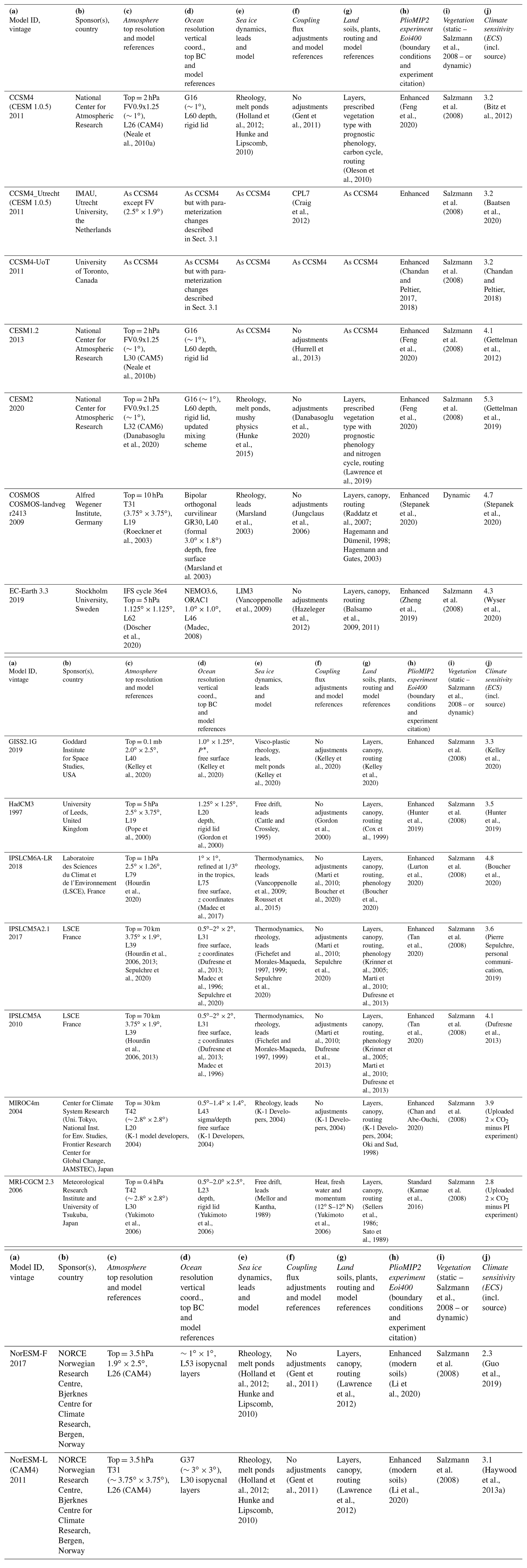
There are currently 16 climate models that have completed the PlioCore experiment to comprise the PlioMIP2 ensemble. These models were developed at different times and have differing levels of complexity and spatial resolution. A further model HadGEM3 is currently running the PlioCore experiment and results from this model will be compared with the rest of the PlioMIP2 ensemble in a subsequent paper. The current 16 model ensemble is double the size of the coupled atmosphere–ocean ensemble presented in the PlioMIP1 large-scale features publication (Haywood et al., 2013a). Summary details of the included models and model physics, along with information regarding the implementation of PRISM4 boundary conditions and each model's ECS, can be found in Tables 1 and S1. Each modelling group uploaded the final 100 years of each simulation for analysis. These were then regridded onto a regular grid using a bilinear interpolation to enable each model to be analysed in the same way. Means and standard deviations for each model were then calculated across the final 50 years.
Table 1Details of climate models used with the PlioCore experiment (a–g) plus details of boundary conditions (h), treatment of vegetation (i) and equilibrium climate sensitivity values (j) (∘C).
2.4 Equilibrium climate sensitivity (ECS) and Earth system sensitivity (ESS)
In Sect. 3.6, we use the PlioCore and PICtrl simulations to investigate ECS and ESS. The PlioCore experiments represent a 400 ppmv world that is in quasi-equilibrium with respect to both climate and ice sheets and hence represents an “Earth system” response to the 400 ppmv CO2 forcing. The Earth system response to a doubling of CO2 (i.e. 560–280 ppmv; ESS) can then be estimated as follows:
There will be errors in the estimate of ESS from the above equation; for example, the equation assumes that the sensitivity to CO2 is linear, which may not necessarily be the case. Further errors will occur because of changes between PlioCore and PICtrl which should not be included in estimates of ESS, such as land–sea mask changes, topographic changes, changes in soil properties and lake changes. However, all these additional changes are likely minimal compared to the ice sheet and greenhouse gas (GHG) changes and are expected to have only a negligible impact on the globally averaged temperature and therefore the estimate of ESS. For example, Pound et al. (2014) found that the inclusion of Pliocene soils and lake distributions in a climate model had an insignificant effect on global temperature (even though changes regionally could be important).
To assess the relationship across the ensemble between the reported ECS and the modelled ESS, we correlate reported ECS across the ensemble with the associated PlioCore–PICtrl temperature anomalies. We do this on global, zonal mean and local scales. A strong correlation at a particular location would suggest that MP proxy data at that location could be used to derive proxy-data-constrained estimate of ECS (similar to an emergent constraint), while a weak correlation would suggest that proxy data at that location could not be used in ECS estimates.
3.1 Surface air temperature (SAT)
Figure 1a shows the global mean surface air temperature (SAT) for each model. The top panel shows the PlioCore and PICtrl SATs, while the lower panel shows the anomaly between them. In this and all subsequent figures, the models are ordered by ECS (see Table 2) such that the model with the highest published ECS (i.e. CESM2; ECS=5.3) is shown on the left, while the model with the lowest published ECS (i.e. NorESM1-F; ECS=2.3) is on the right. Increases in PlioCore global annual mean SATs, compared to each of the contributing models PICtrl experiment, range from 1.7 to 5.2 ∘C (Fig. 1a; Table 2) with an ensemble mean ΔT of 3.2 ∘C. The multi-model median ΔT is 3.0 ∘C, while the 10th and 90th percentiles are 2.1 and 4.8 ∘C respectively. Analogous results from individual models of the PlioMIP1 ensemble are shown by the horizontal grey lines in Fig. 1a and have a mean warming of 2.7 ∘C. Pliocene warming for individual PlioMIP1 models falls into two distinct anomaly bands that are 1.8–2.2 ∘C (CCSM4, GISS-E2-R, IPSLCM5A, MRI2.2) and 3.2–3.6 ∘C (COSMOS, HadCM3, MIROC4m, NorESM-L). PlioMIP2 shows a greater range of responses than PlioMIP1, and PlioMIP2 results are more evenly scattered over the ensemble range. The ensemble mean temperature anomaly is larger in PlioMIP2 than in PlioMIP1 because of the addition of new and more sensitive models to PlioMIP2 rather than being due to the change in boundary conditions between PlioMIP1 and PlioMIP2.
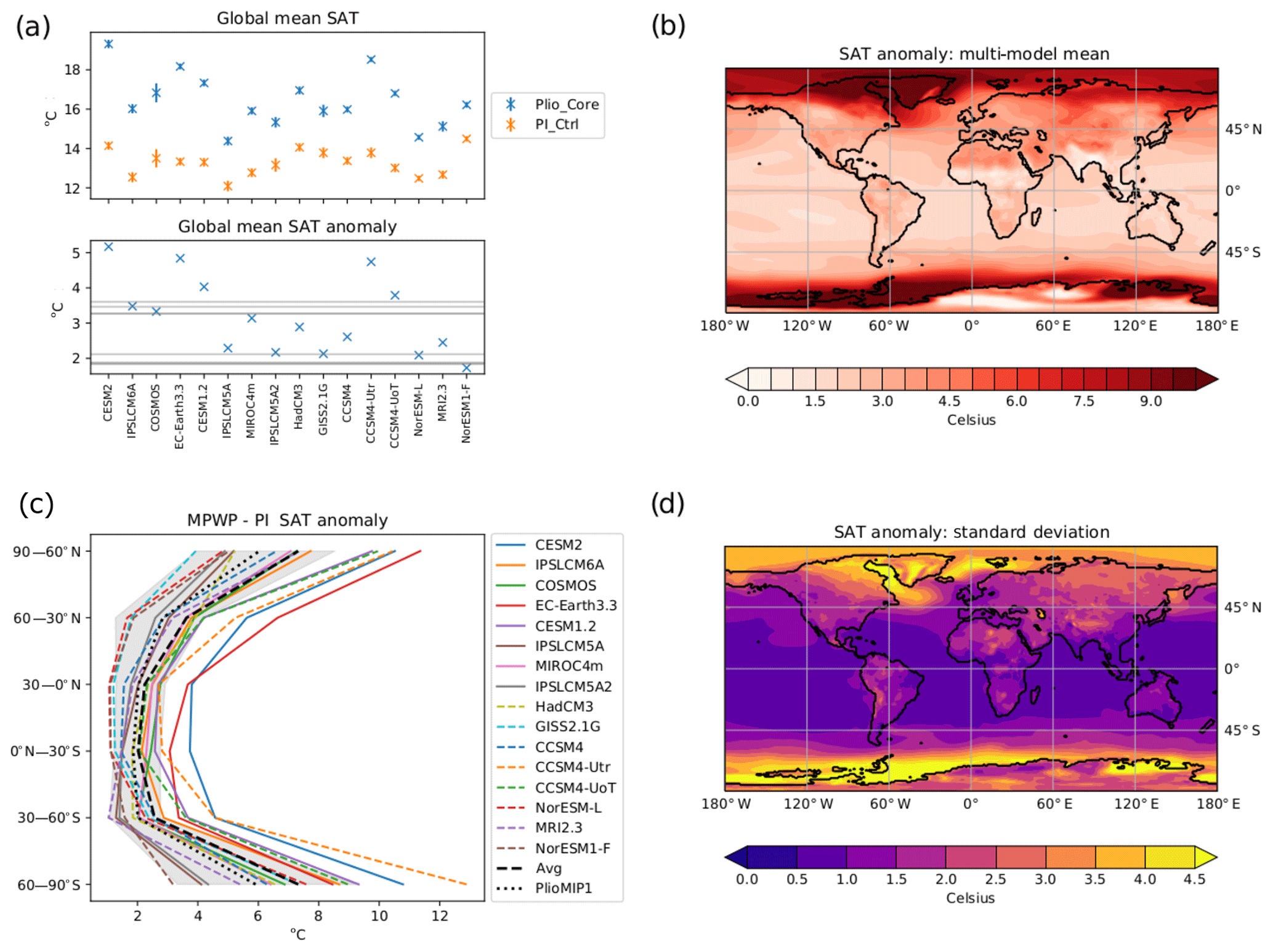
Figure 1(a) Global mean near-surface air temperature (SAT) for the PlioCore and PICtrl experiments from each PlioMIP2 model (upper panel) and the difference between them (PlioCore–PICtrl) (lower panel). Crosses show the mean value, while the vertical bars show the inter-annual standard deviation. Horizontal grey lines on the lower panel show the anomalies from individual PlioMIP1 models. (b) Multi-model mean PlioCore–PICtrl SAT anomaly. (c) Latitudinal mean PlioCore–PICtrl SAT anomaly from each PlioMIP2 model. The PlioMIP2 multi-model mean is shown by the dashed black line. The grey shaded area shows the range of values of the PlioMIP1 models. The PlioMIP1 multi-model mean is shown by the dotted black line. (d) Intermodel standard deviation for the PlioCore–PICtrl anomaly.
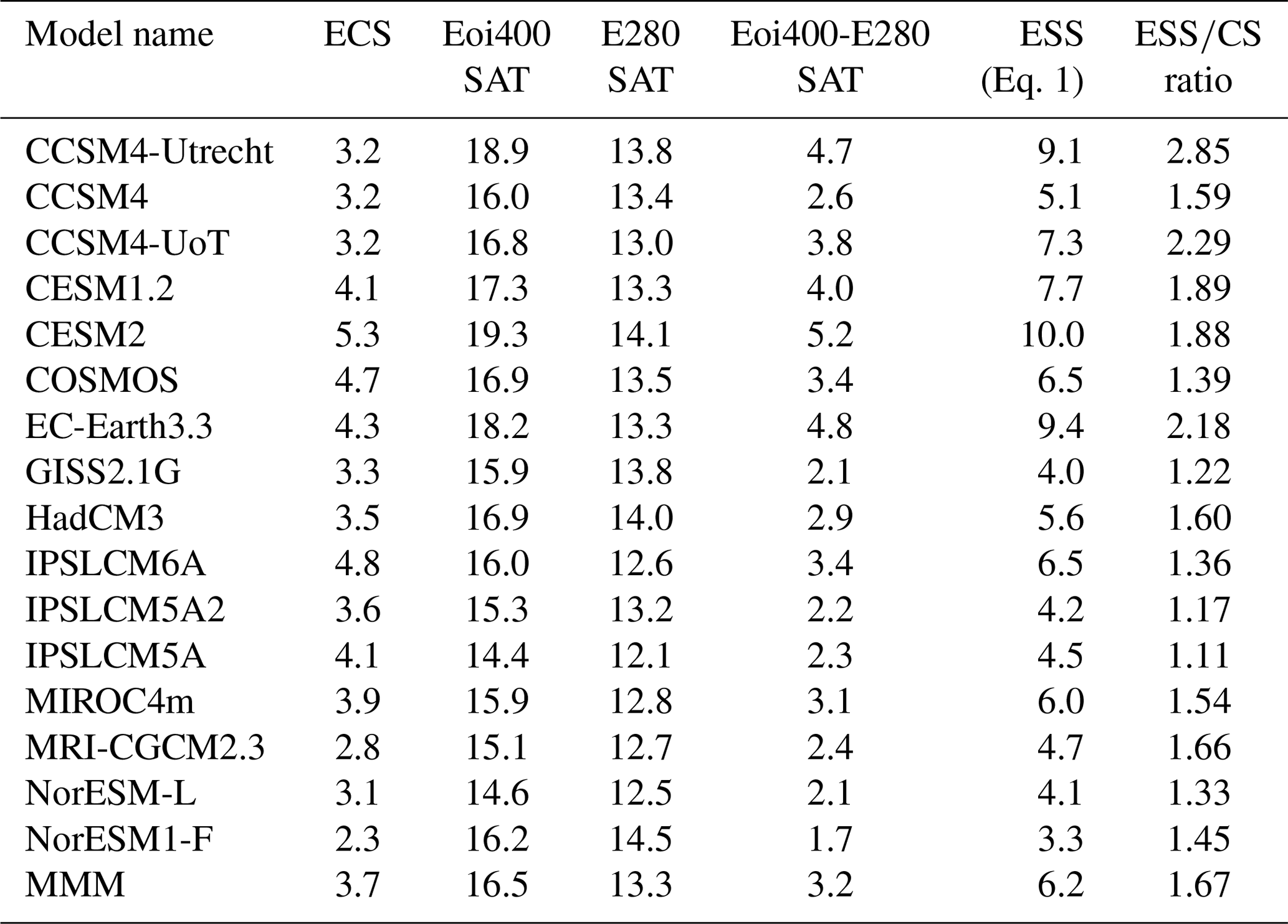
Table 2Details of the relationship between the equilibrium climate sensitivity (ECS) and the Earth system sensitivity (ESS) for each model. MMM denotes the multi-model mean.
PlioMIP2 shows increased SATs over the whole globe (Fig. 1b) with an ensemble average warming of ∼2.0 ∘C for the tropical oceans (20∘ N–20∘ S), which increases towards the high latitudes (Fig. 1b, c). Multi-model mean SAT warming can exceed 12 ∘C in Baffin Bay and 7 ∘C in the Greenland Sea (Fig. 1b), a result potentially influenced by the closure of the Canadian Archipelago and Bering Strait, as well as by the specified loss of most of the Greenland Ice Sheet (GIS) and the simulated reduction in Northern Hemisphere sea-ice cover (de Nooijer et al., 2020). In the Southern Hemisphere, warming is pronounced in regions of Antarctica that were deglaciated in the MP in both west and east Antarctica (Fig. 1b). Warming in the interior of east Antarctica is limited by the prescribed topography of the MP East Antarctic Ice Sheet (EAIS), which in some places exceeds the topography of the EAIS in the models' PICtrl experiments.
In terms of magnitude, the CESM2 model has the greatest apparent sensitivity to imposing MP boundary conditions with a simulated ΔT of 5.2 ∘C (Fig. 1a). This model was published in 2020 and has the highest ECS of all the PlioMIP2 models. This model was not included in PlioMIP1, and its response to Pliocene boundary conditions lies outside the range of all PlioMIP1 models both in global mean and for every latitude band (Fig. 1a, c). It is also warmer than the PlioMIP2 multi-model mean in nearly all grid boxes (Fig. S1 in the Supplement). Other particularly sensitive models (EC-Earth3.3, CESM1.2, CCSM4-Utr and CCSM4-UoT; shown as an anomaly from the multi-model mean in Fig. S1) are also new to PlioMIP2, and this explains why the simulated ΔT from PlioMIP2 exceeds that from PlioMIP1. The model with the lowest response to PlioMIP2 boundary conditions is the NorESM1-F model, which is also the model with the lowest published ECS. Although there is clearly some correlation between a model's ECS and its PlioCore–PICtl temperature anomaly, the relationship is not exact. In particular, the versions of CCSM4 that were run by Utrecht University (CCSM4-Utr) and the University of Toronto (CCSM-UoT) both show a large Pliocene response but have a modest ECS compared to the other models.
Three different versions of CCSM4 contributed to PlioMIP2 (see Table 1): the standard version run at the National Center for Atmospheric Research (NCAR) (hereafter referred to as CCSM) has a simulated ΔT=2.6 ∘C, while CCSM4-Utr has a simulated ΔT=4.7 ∘C, and CCSM4-UoT has a simulated ΔT=3.8 ∘C. A notable difference between these simulations is the response in the 60–90∘ S band where the mean warming in the CCSM4-Utr simulation is 4 ∘C higher than in the CCSM4-UoT simulation and 6.6 ∘C higher than in the CCSM4 simulation (Figs. 1c, S1). Table S1 shows that, even though the CCSM4 models differ in their response, they all appear to be close to equilibrium. In addition, they are all reported to have similar ECSs (Table 1), and they all have the same physics apart from changes to the standard ocean model in the CCSM4-UoT simulations and the PlioCore CCSM4-Utr simulation. These changes (discussed by Chandan and Peltier, 2017, this special issue) are as follows: (1) the vertical profile of background diapycnal mixing has been fixed to a hyperbolic tangent form, and (2) tidal mixing and dense water overflow parameterization schemes have been turned off. Although the exact cause of the differences in ΔT between the CCSM4 models remains unclear, the changes in the ocean parameterizations and differences in initialization may contribute to the ΔT differences, in particular the changes in ocean mixing between different versions of the model (Fedorov et al., 2010).
Analysis of the standard deviation of the model ensemble (Fig. 1d) indicates that models are generally consistent in terms of the magnitude of temperature response in the tropics, especially over the oceans. However, they can differ markedly in the higher latitudes where the inter-model standard deviation reaches more than 4.5 ∘C.
To evaluate whether the multi-model mean PlioCore–PICtrl anomaly at a grid box is “robust” we follow the methodology of Mba et al. (2018) and Nikulin et al. (2018). The anomaly is said to be robust if two conditions are fulfilled: (1) at least 80 % models agree on the sign of the anomaly, and (2) the signal-to-noise ratio (i.e. the ratio of the size of the mean anomaly to the inter-model standard deviation; Fig. 1b, d) is greater than or equal to 1. Regions where the SAT anomaly is considered robust according to these criteria are hatched in Fig. 2. It is seen that for SAT the PlioCore–PICtrl anomaly is considered robust across the ensemble over nearly all the globe.
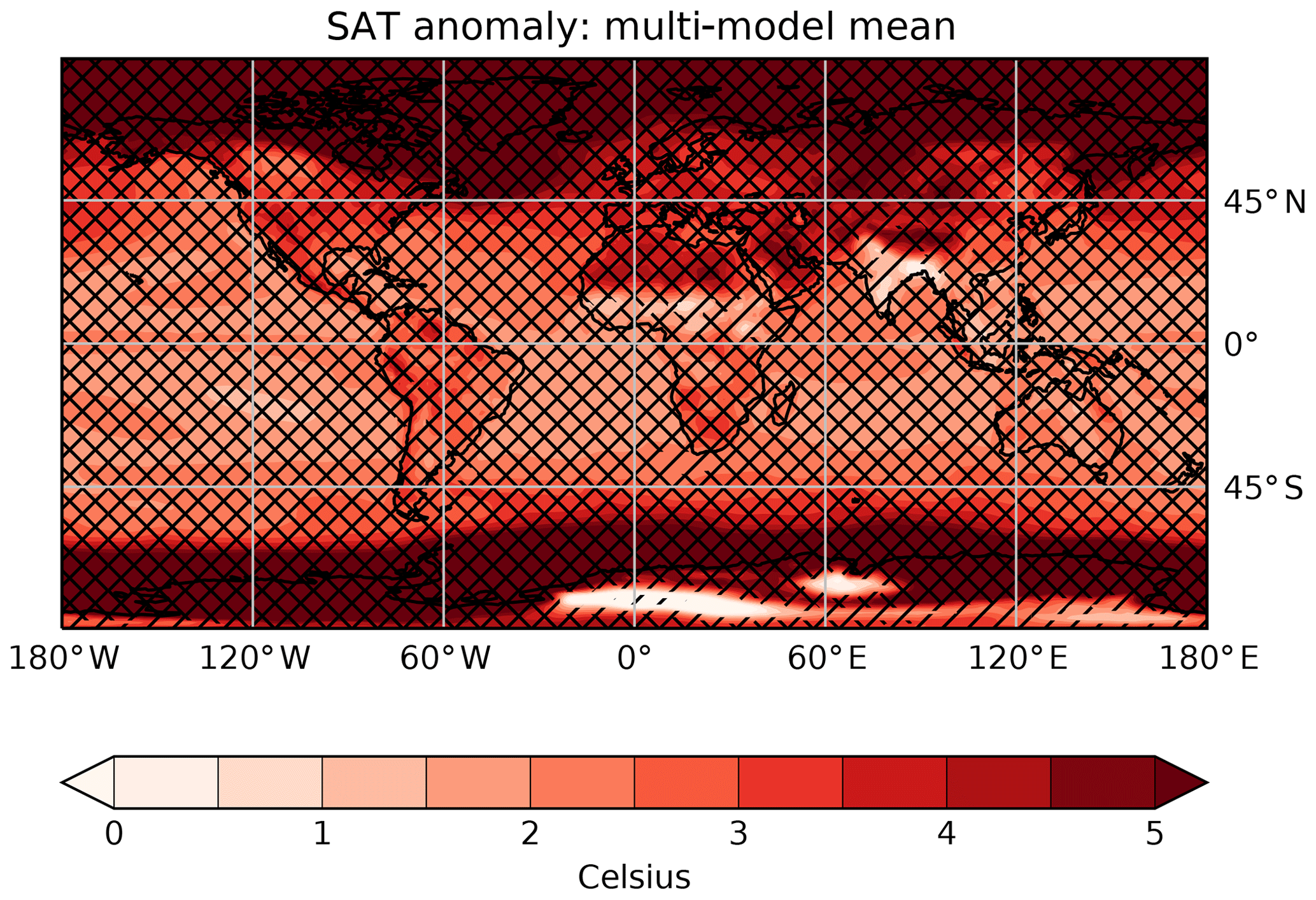
Figure 2PlioCore–PICtrl SAT multi-model mean anomaly. Grid boxes where at least 80 % of the models agree on the sign of the change are marked “∕”. Grid boxes where the ratio of the multi-model mean SAT change to the PICtrl intermodel standard deviation is greater than 1 are marked “\”. Grid boxes where both these conditions are satisfied show a robust signal.
3.2 Seasonal cycle of surface air temperature, land–sea temperature contrasts and polar amplification
The Northern Hemisphere (NH) averaged SAT anomaly over the seasonal cycle is presented in Fig. 3a. Overall, the ensemble mean anomaly (dashed black line) is fairly constant throughout the year; however, models within the ensemble have very different characteristics in terms of the monthly and seasonal distribution of the warming. Some members of the ensemble have a relatively flat seasonal cycle in ΔSAT (e.g. NorESM-L, NorESM1-F, COSMOS); however, others show a very strong seasonal cycle. The models that show a very strong seasonal cycle do not agree on the timing of the peak warming. For example, EC-Earth3.3 has the peak warming in October, CESM2 has peak warming in July, and MRI2.3 has peak warming in January/February. The lack of consistency in the seasonal signal of warming has interesting implications in terms of whether PlioMIP2 outputs could be used to examine the potential for seasonal bias in proxy datasets. To do this meaningfully would require clear consistency in model seasonal responses, which is absent in the PlioMIP2 ensemble. The grey shaded area in Fig. 3a shows the range of NH temperature responses in PlioMIP1, with the PlioMIP1 ensemble average shown by the dotted black line. Although the ensemble average from both PlioMIP2 and PlioMIP1 shows a relatively flat seasonal cycle, the range of responses is very different between the two ensembles. PlioMIP1 predicted a large range of temperature responses in the NH winter, which reduced in the summer. In PlioMIP2, however, the summer range is amplified compared to the winter. Indeed 7 of the 16 PlioMIP2 models show a NH summer temperature anomaly that is noticeably above that seen in any of the PlioMIP1 simulations. Some of these models (CESM2, EC-Earth3.3, CCSM4-Utr, CCSM4-UoT and CESM1.2) did not contribute to PlioMIP1, which shows that whichever models are included in an ensemble can strongly affect the ensemble response. However, other models (MIROC4m and HadCM3) that show an enhanced summer response in PlioMIP2 were also included in PlioMIP1, showing that there is also an impact of the change in boundary conditions on seasonal temperature. None of the PlioMIP2 models replicate the lowest warming seen in December–February (DJF) in the PlioMIP1 ensemble; this lowest value was derived from the GISS-E2-R model in PlioMIP1 which did not contribute to PlioMIP2.
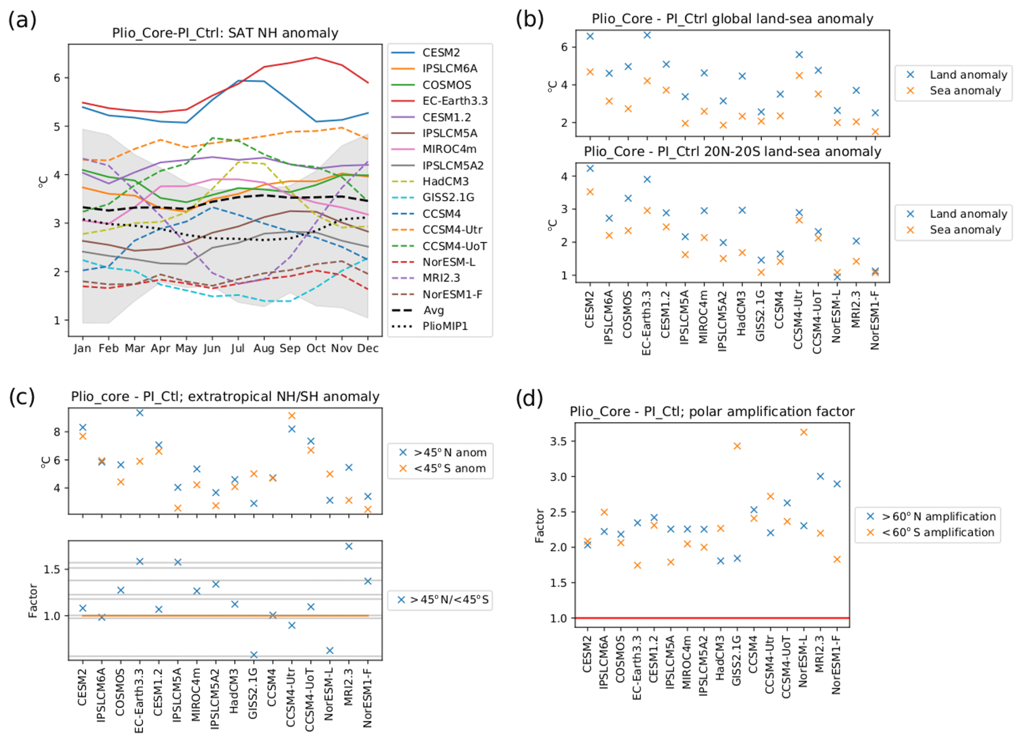
Figure 3(a) Monthly mean NH PlioCore–PICtrl SAT anomaly for each PlioMIP2 model, with the PlioMIP2 multi-model mean shown by the dashed black line. The grey shaded region shows the range of values simulated by the PlioMIP1 models, and the PlioMIP1 multi-model mean is shown by the dotted black line. (b) SAT anomaly for land (blue) and sea (orange) from each model averaged over the globe (top panel) and the 20∘ N–20∘ S region (lower panel). (c) SAT anomaly for the northern extratropics (blue) and southern extratropics (orange) (top panel) and the ratio between them (lower panel). The horizontal grey lines on the lower panel show the values from individual PlioMIP1 models. (d) SAT anomaly poleward of 60∘ divided by the globally averaged SAT anomaly for the NH (blue) and the SH (orange). The red line highlights a ratio of 1 (i.e. no polar amplification).
The ensemble results for land–sea temperature contrasts clearly indicate a greater warming over land than over the oceans (Fig. 3b). This result also holds when only the land–sea temperature contrast in the tropics is considered. The land amplification factor is similar in PlioMIP2 and PlioMIP1, and models in both ensembles cluster near a land amplification factor of ∼1.5. There is also no relationship between a model's climate sensitivity and the land amplification factor. The multi-model median (10th percentile/90th percentile) warming over the land and ocean is 4.5 ∘C (2.6 ∘C/6.1 ∘C) and 2.5 ∘C (1.9 ∘C/4.4 ∘C) respectively.
The extratropical NH (45–90∘ N) warms more than the extratropical Southern Hemisphere (SH) (45–90∘ S) in 5 of the 8 models (62 %) from PlioMIP1 and in 11 of the 16 models (69 %) from PlioMIP2 (Fig. 3c). This shows that neither the change in boundary conditions nor the addition of newer models to PlioMIP2 affects the ensemble proportion of enhanced NH warming; nor does the published ECS have any obvious impact on whether the warming is concentrated in the NH or the SH. The models that indicate greater SH versus NH warming (CCSM4-Utr, GISS2.1G, NorESM-L) are among those that have weaker differences between land and ocean warming (Fig. 3b).
Polar amplification (PA) can be defined as the ratio of polar warming (poleward of 60∘ in each hemisphere) to global mean warming (Smith et al., 2019). The PA for each model for the NH and the SH is shown in Fig. 3d. All models show PA>1 for both hemispheres, although whether there is more PA in the NH or SH is a model-dependent feature. The ensemble mean (median) PA is 2.3 (2.2) in both the NH and the SH, suggesting that across the ensemble PA is hemispherically symmetrical. This result is very similar to PlioMIP1 (not shown), which suggests that the enhanced warming in the PlioMIP2 ensemble does not affect the PA. For PlioMIP2, the NH median PA is 2.2 with the 10th and 90th percentiles at 1.9 and 2.8 respectively, while in the SH the median PA is 2.2, with the 10th and 90th percentiles at 1.8 and 3.1 respectively. Polar amplification is lower over the land than the ocean (Fig. S2) in both hemispheres. The NH mean (10th ∕ 50th ∕ 90th percentiles) PAs are 1.6 () and 2.7 () over the land and ocean respectively, while the SH mean (10th ∕ 50th ∕ 90th percentiles) PAs are 0.9 () and 1.9 () over the land and ocean respectively. Note that in the SH total PA is higher than both land and ocean PAs because of the change in the area of land between the PlioCore and PICntl experiments. There appears to be a weak relationship between the PA factor and a model's ECS. Those models which have a lower published ECS (those to the right of Fig. 3d) have a tendency towards a higher PA. This is not because these models have excess warming at high latitudes, but rather these models have less tropical warming than other models.
3.3 Meridional/zonal SST gradients in the Pacific and Atlantic
There has been great interest in the reconstruction of Pliocene SST gradients in the Atlantic and Pacific to provide first order assessments of Pliocene climate change and to assess possible mechanisms of Pliocene temperature enhancement and ocean–atmospheric dynamic responses (Rind and Chandler, 1991). For example, the meridional gradient in the Atlantic has been discussed in terms of the potential for enhanced ocean heat transport in the Pliocene (e.g. Dowsett et al., 1992). In addition, the zonal SST gradient across the tropical Pacific has been used to examine the potential for change in Walker Circulation and, through this, El Niño–Southern Oscillation (ENSO) dynamics and teleconnection patterns during the Pliocene (Fedorov et al., 2013; Burls and Fedorov, 2014; Tierney et al., 2019).
The multi-model mean meridional profile of zonal mean SSTs in the Atlantic Ocean is shown in Fig. 4a. In the tropics and subtropics, the SST increase between the PlioCore and PICtrl experiments is 1.5–2.5 ∘C. This difference increases to ∼5.0 ∘C in the NH at ∼55∘ N with an inter-model range of 2–11 ∘C. The Pliocene and pre-industrial meridional SST profile in the Pacific (Fig. 4b) is similar to that of the Atlantic but with little indication from the multi-model mean for a high-latitude enhancement in meridional temperature. However, a large range in the ensemble response is noted, and the importance of an adjustment of the vertical mixing parameterization towards the simulation of a reduced Pliocene meridional gradient has recently been shown (Lohmann et al., 2020).
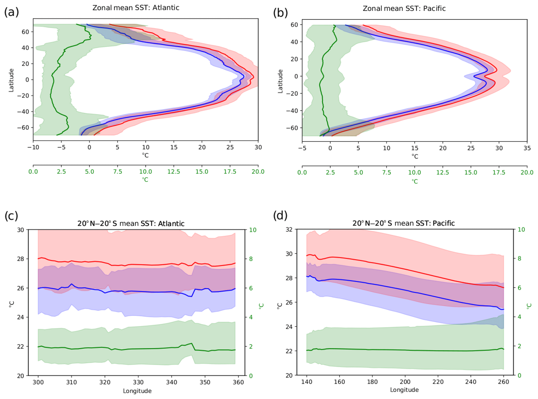
Figure 4Panels (a, b) show the zonally averaged SST over the Atlantic region (70∘ W–0∘ E) and the Pacific region (150∘ E–100∘ W) respectively. Panels (c, d) show the SST averaged between 20∘ N and 20∘ S for the Atlantic and Pacific respectively. In all figures, blue shows PICtrl, red shows PlioCore and green shows the anomaly between them. The solid line shows the multi-model mean, while the shaded area shows the range of modelled values.
In the tropical Atlantic (20∘ N–20∘ S), the multi-model mean zonal mean SST for the Pliocene increases by ∼1.9 ∘C (ensemble range from 0.8 to 3–4 ∘C) with a flat zonal temperature gradient across the tropical Atlantic (Fig. 4c). In the tropical Pacific, both Pliocene and pre-industrial ensembles clearly show the signature of both a western Pacific warm pool and the relatively cool waters in the eastern Pacific that are associated with upwelling (Fig. 4d). As such, a clear east–west temperature gradient is evident in the Pliocene tropical Pacific in the PlioMIP2 ensemble (similar to PlioMIP1) and is not consistent with a permanent El Niño (see Fig. S3). The PlioMIP2 ensemble supports a recent proxy-derived reconstruction for the Pacific that found Pliocene ocean temperatures increased in both the eastern and western tropical Pacific (Tierney et al., 2019).
Using the methodology of Mba et al. (2018) and Nikulin et al. (2018), the signal of SST change seen in the multi-model mean is robust over nearly all ocean grid cells (Fig. S4). Figure S3 shows the difference between the Pliocene ΔSST for each model in the PlioMIP2 ensemble and the Pliocene ΔSST of the multi-model mean. This illustrates that, despite the climate anomaly being larger than the inter-model standard deviation, there are still many regions (e.g. Southern Ocean, North Atlantic Ocean, Arctic Ocean) where there is a notable inter-model spread of the magnitude of the Pliocene SST anomalies.
3.4 Total precipitation rate
Simulated increases in PlioCore global annual mean precipitation rates compared to each contributing model's PICtrl experiment (hereafter referred to as ΔPrecip) range from 0.07 to 0.37 mm d−1 (Fig. 5a), which is notably larger than the PlioMIP1 range of 0.09–0.18 mm d−1 (shown as horizontal grey lines in Fig. 5a). The PlioMIP2 ensemble mean ΔPrecip is 0.19 mm d−1. The increase in the globally averaged precipitation anomaly in PlioMIP2 is due to the addition of new models to the ensemble which have high ECS and are also more sensitive to the PlioMIP2 boundary conditions. Models that were included in PlioMIP1 (COSMOS, IPSLCM5A, MIROC4m, HadCM3, CCSM4, NorESM-L and MRI2.3) show PlioMIP2 precipitation anomalies that are similar to PlioMIP1 results. The spatial pattern (Fig. 5b) shows enhanced precipitation over high latitudes and reduced precipitation over parts of the subtropics. The largest ΔPrecip is found in the tropics in regions of the world that are dominated by the monsoons (west Africa, India, East Asia). The enhancement in precipitation over northern Africa is consistent with previous Pliocene modelling results that have demonstrated a weakening in Hadley circulation linked to a reduced pole-to-Equator temperature gradient (e.g. Corvec and Fletcher, 2017). Greenland shows increased PlioCore precipitation in regions that have become deglaciated and are therefore substantially warmer. Latitudes associated with the westerly wind belts also show enhanced PlioCore precipitation with an indication of a poleward shift in higher-latitude precipitation. This result is consistent with findings from PlioMIP1 (Li et al., 2015). Other, more locally defined examples of ΔPrecip appear closely linked to localized variations in Pliocene topography and land–sea mask changes, for example, the Sahul and Sunda shelves that become subaerial in the PlioCore experiment. In general, the models that display the largest SAT sensitivity to the prescription of Pliocene boundary conditions also display the largest ΔPrecip (CESM2, CCSM4-Utr, EC-Earth3.3). This is consistent with a warmer atmosphere leading to a greater moisture carrying capacity and therefore greater evaporation and precipitation. The model showing the least sensitivity in terms of precipitation response is GISS2.1G.
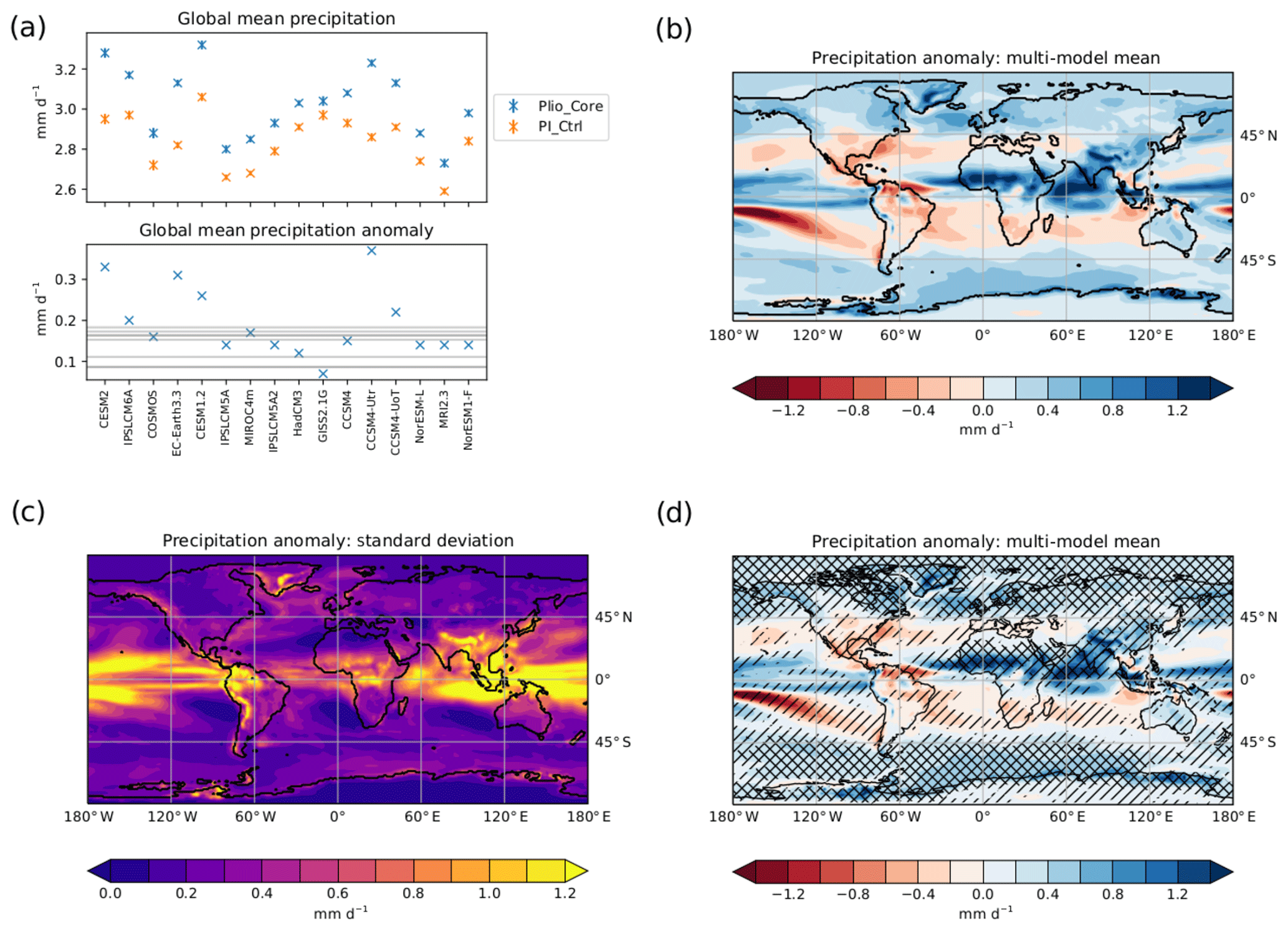
Figure 5(a) Globally averaged precipitation for PlioCore and PICtrl from each model (upper panel) and the anomaly between them (lower panel). The horizontal grey lines in the lower panel show the values that were obtained from each individual PlioMIP1 model. (b) Multi-model mean PlioCore–PICtrl precipitation anomaly. (c) Standard deviation across the models for the PlioCore–PICtrl precipitation anomaly. (d) PlioCore–PICtrl precipitation anomaly. Regions which have at least 80 % of the models agreeing on the sign of the change are marked with “∕”. Regions where the ratio of the multi-model mean precipitation change to the PICtrl intermodel standard deviation is greater than 1 are marked with “\”.
Analysis of the standard deviation within the ensemble demonstrates that, in contrast to SAT, models are most consistent regarding ΔPrecip in the extratropics (Fig. 5c). This is similar to the findings of PlioMIP1 (Haywood et al., 2013a) and is likely because more precipitation falls in the tropics than extratropics, and therefore the inter-model differences are larger in the tropics. The methodology of Mba et al. (2018) and Nikulin et al. (2018) (described in Sect. 3.1) was used to determine the robustness of ΔPrecip (Fig. 5d). Unlike the temperature signal, which was robust throughout most of the globe, there are large regions in the tropics and subtropics where the ensemble precipitation signal is uncertain. Changes in precipitation rates in the subtropics have some inter-model coherence in many places because at least 80 % of models agree on the sign of change. However, most of these predicted changes are not robust because the magnitude of change is not large compared to the standard deviation seen in the ensemble (Fig. 5c). This is consistent with results from CMIP5, which show that predicted precipitation changes have low confidence particularly in the low and medium emissions scenarios (IPCC, 2013). The signal of precipitation change is determined to be robust in the high latitudes and in the middle latitudes in regions influenced by the westerlies. This is also the case in regions influenced by the west African, Indian and East Asian summer monsoons (Fig. 5d). Figure S5 shows the difference between each model's ΔPrecip and the multi-model mean ΔPrecip (shown in Fig. 5b), highlighting that there is uncertainty in the ensemble with respect to the regional patterns of precipitation change.
3.5 Seasonal cycle of total precipitation and land–sea precipitation contrasts
Figure 6a shows the seasonal cycle of the precipitation anomaly averaged over the Northern Hemisphere. As was the case for SAT, the monthly and seasonal distribution of precipitation anomalies is highly model dependent, although the ensemble average shows a clear NH late spring to autumn PlioCore enhancement in precipitation (Fig. 6a). This is most strongly evident in the models CESM2, EC-Earth3.3 and CCSM4-Utr; however, it is also evident in other models. Some models show a different seasonal cycle to the ensemble mean, for example, the GISS2.1G model, which simulates the NH late spring to autumn ΔPrecip being suppressed compared to the rest of the year, and HadCM3, which has a bimodal distribution. An increase in NH summer precipitation is consistent with a general trend of west African, Indian and East Asian summer monsoon enhancement, and this will be discussed in detail in a forthcoming PlioMIP2 paper. In PlioMIP1 (ensemble average – dotted black line and model range – grey shaded area in Fig. 6a), the seasonal cycle in precipitation was much more muted. PlioMIP1 results in boreal winter are similar to PlioMIP2; however, the mean precipitation anomaly in PlioMIP2 between June and November is 40 % larger than PlioMIP1. This increase is mainly due to the inclusion of new and more sensitive models into PlioMIP2 (e.g. CESM2 and EC-Earth3.3). However, some models with enhanced summer precipitation (e.g. COSMOS) contributed to both PlioMIP1 and PlioMIP2, suggesting a role of boundary condition changes in enhancing the NH boreal summer precipitation. It is noted, however, that not all the new models in PlioMIP2 show enhanced summer precipitation relative to PlioMIP1. The GISS2.1G model, which was new to PlioMIP2, shows the most muted summer precipitation response in the NH in all PlioMIP2 and PlioMIP1 models. This means that the range of summer–autumn NH precipitation responses as shown by the ensemble increases significantly in PlioMIP2. For example, PlioMIP1 showed a NH precipitation response in October to be 0.13–0.42 mm d−1, while in PlioMIP2 this has increased to 0.05–0.70 mm d−1.
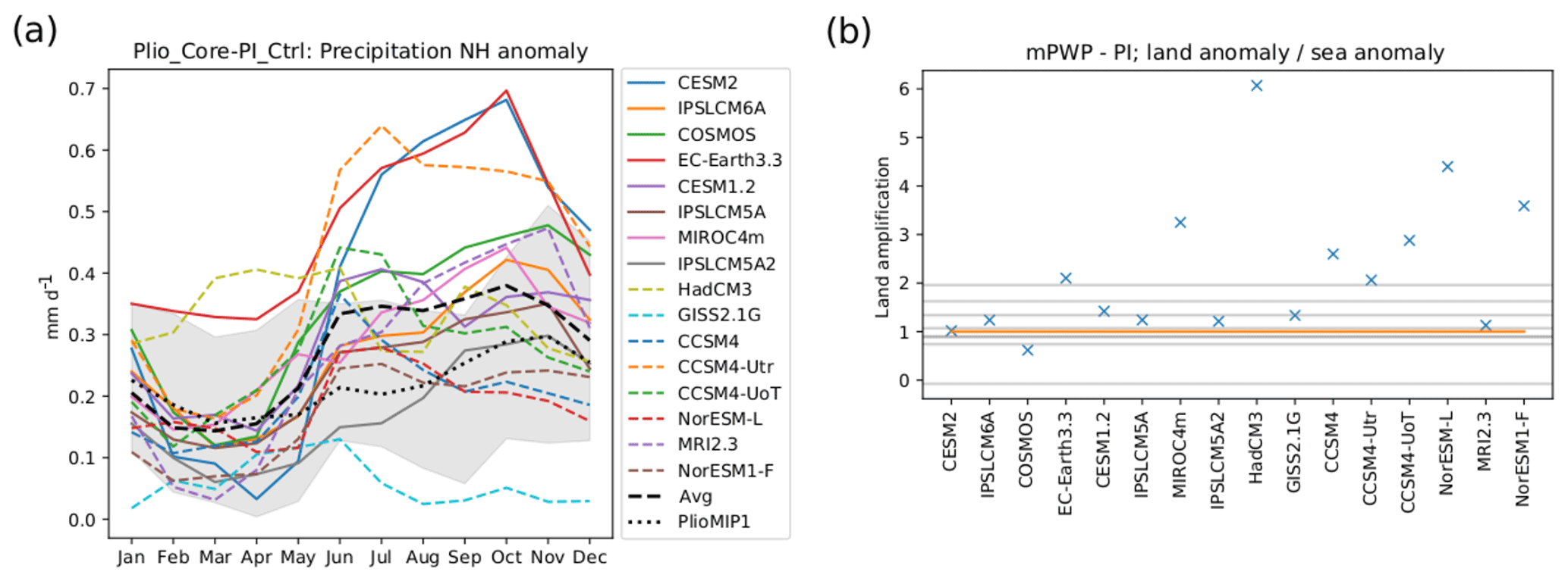
Figure 6(a) The NH averaged precipitation anomaly for each PlioMIP2 model and for each month with the dashed black line showing the PlioMIP2 multi-model mean. The grey shaded region shows the range of values obtained from PlioMIP1 with the PlioMIP1 multi-model mean shown by the dotted black line. (b) The ratio of the precipitation anomaly over land to the precipitation anomaly over sea for each PlioMIP2 model. Analogous results from individual PlioMIP1 models are shown by the thin grey lines. A ratio of 1.0, where the land precipitation anomaly is the same as the sea precipitation anomaly, is shown in orange.
In terms of the land–sea ΔPrecip contrast, the PlioMIP2 ensemble divides into two groups (Fig. 6b), one in which a clear pattern of precipitation anomaly enhancement over land compared to the oceans is seen (EC-Earth3.3, MIROC4m, HadCM3, CCSM4, CCSM4-Utr, CCSM4-UoT, NorESM-L and NorESM-F) and the other in which there is either a small or no enhancement in the land versus oceans (CESM2, IPSLCM6A, COSMOS, CESM1.2, IPSLCM5A, IPSLCM5A2, GISS2.1G and MRI2.3). Models which show the greatest precipitation enhancement over the land are generally those which have a lower published ECS (those to the right of Fig. 6b) and a small precipitation response over the oceans but a land precipitation anomaly similar to other models. Models with a higher ECS (e.g. CESM2) show a similar precipitation anomaly over the land and ocean. The horizontal grey lines in Fig. 6b show the land–sea ΔPrecip amplification for the PlioMIP1 models. None of the PlioMIP1 models have a ΔPrecip amplification factor >2; however, half of the PlioMIP2 models do. Further, four models which contributed to both PlioMIP1 and PlioMIP2 (MIROC4m, HadCM3, CCSM4, NorESM-L) have a much greater land amplification in PlioMIP2, showing that the change in boundary conditions strongly affects this diagnostic.
3.6 Climate and Earth system sensitivity
This section will consider the relationship between ECS and ESS across the ensemble. Table 2 shows the ECS for each model (referenced in Table 1) and the ESS estimated from the PlioCore–PICtrl temperature anomaly (Eq. 1). Since ice sheet changes were prescribed, there will be no transient response due to ice sheet changes, and the PlioCore experiment will be in equilibrium with the ice sheets. The mean ESS∕ECS ratio is 1.67, suggesting that the ESS based on the ensemble is 67 % larger than the ECS; however, the range is large with the GISS2.1G model suggesting that the ESS∕ECS ratio is 1.22, while the CCSM4_Utr model suggests that the ESS∕ECS ratio is 2.85.
The first analysis of how ECS relates to ESS will consider the correlation between ECS and the globally averaged PlioCore–PICtrl temperature anomaly. This is seen in Fig. 7a, and each cross represents the results from a different model in the PlioMIP2 ensemble. There is a significant relationship between ECS and the PlioCore–PICtrl temperature anomaly at the 95 % confidence level (p=0.01, R2=0.35) with the line of best fit being .

Figure 7(a) The globally averaged PlioCore–PICtrl SAT anomaly for each model versus the published equilibrium climate sensitivity (crosses) with the line of best fit shown in orange. (b) Statistical relationships between the latitudinally averaged PlioCore–PICtrl SAT anomaly and the published climate sensitivity. The proportion of climate sensitivity that can be explained by the SAT anomaly at each latitude (R2) is shown in red, while the probability that there is no correlation between the climate sensitivity and the SAT anomaly (p) is shown in blue. (c) Colours show the percentage variation in modelled ECS that is linearly related to the modelled PlioCore–PICtrl SAT anomaly at each grid square (R2). Hatching shows a significant relationship (at the 5 % confidence level) between the PlioCore–PICtrl SAT anomaly at that grid square and ECS.
Next, we investigate whether there is a correlation across the ensemble between ECS and the PlioCore–PICtrl SAT anomaly on spatial scales. In the analysis that follows, we will simply assess whether such a correlation exists and, if so, how strong it is by looking at p values and R-squared values calculated from the models in the ensemble. Figure 7b shows the relationship (p value – blue, R squared – red) across the ensemble between modelled ECS and the modelled zonal mean PlioCore–PICtrl SAT anomaly. We find a significant relationship (p<0.05) between ECS and the zonal mean Pliocene temperature anomaly throughout most of the tropics. This relationship becomes significant at the 99 % confidence level (p<0.01) between 38∘ N and 27∘ S, where a high proportion of the inter-model variability in global ECS can be related to the inter-model variability in the Pliocene SAT anomaly at an individual latitude, reaching a maximum of 65 % at ∼15∘ N.
Next the relationship between global ECS and the local PlioCore–PICtrl SAT anomaly is assessed. In Fig. 7c, colours show the R-squared correlation across the ensemble between modelled global ECS and the modelled local PlioCore–PICtrl SAT anomaly. The regions where the relationship between the two is significant at the 95 % confidence level are hatched. The relationship between ECS and the local PlioCore–PICtrl SAT anomaly is significant over most of the tropics and over some middle- and high-latitude regions including Greenland and parts of Antarctica. In many cases, the tropical oceans show a temperature anomaly more strongly related to ECS than the land, although this is not always the case.
Haywood et al. (2013a, b) proposed that the proxy data and climate model comparison in PlioMIP1 could include discrepancies owing to the comparison between time averaged PRISM3D SST and SAT data and climate model representations of a single time slice. In order to improve the integrity of the data–model comparisons in PlioMIP2, Foley and Dowsett (2019) synthesized alkenone SST data that can be confidently attributed to the Marine Isotope Stage (MIS) KM5c time slice that experiment PlioCore is designed to represent. Foley and Dowsett (2019) provide two different SST datasets. One dataset includes all SST data for an interval of 10 000 years around the time slice (5000 years to either side of the peak of MIS KM5c), and the other covers 30 000 years (up to 15 000 years to either side of the peak; this latter dataset will hereafter be referred to as F&D19_30). Age models used in the compilation are those originally released with the datasets, but later modifications of age models or the integration of additional data could result in mean SST values different from those reported in F&D19_30. All SST estimates are calibrated using Müller et al. (1998). Prescott et al. (2014) demonstrated that due to the specific nature of orbital forcing 20 000 years before and after the peak of MIS KM5c, age and site correlation uncertainty within that interval would be unlikely to introduce significant errors into SST-based DMC. Given this and in order to maximize the number of ocean sites where SST can be derived, we carry out a point-based SST data–model comparison using the F&D19_30 dataset.
We compare the multi-model mean SST anomaly to a proxy SST anomaly created by differencing the F&D19_30 dataset from observed pre-industrial SSTs derived for years 1870–1899 of the NOAA Extended Reconstructed Sea Surface Temperature (ERSST) version 5 dataset (Huang et al., 2017; Fig. 8a and b). Figure 8c shows the proxy data ΔSST minus the multi-model mean ΔSST. Using the multi-model mean results, 17 of the 37 sites show a difference in data–model ΔSST of no greater than ±1 ∘C (Fig. 8c). These are located mostly in the tropics but also include sites in the North Atlantic, along the coastal regions of California and New Zealand, and in the North Pacific. In terms of discrepancies, the clearest and most consistent signal comes from the Benguela upwelling system (off the south-west coast of Africa) where the multi-model mean does not predict the scale of warming seen in three of the four proxy reconstructions. The multi-model mean is insufficiently sensitive in the two Mediterranean Sea sites, along the east coast of North America (Yorktown Formation) and at one location west of Svalbard close to the sea-ice margin. The multi-model mean predicts a warming that is too great at one location off the Florida and Norwegian coasts. No discernible spatial pattern or structure is seen (outside of the Benguela and Mediterranean regions) for sites where the ensemble underestimates or overestimates the magnitude of SST change.
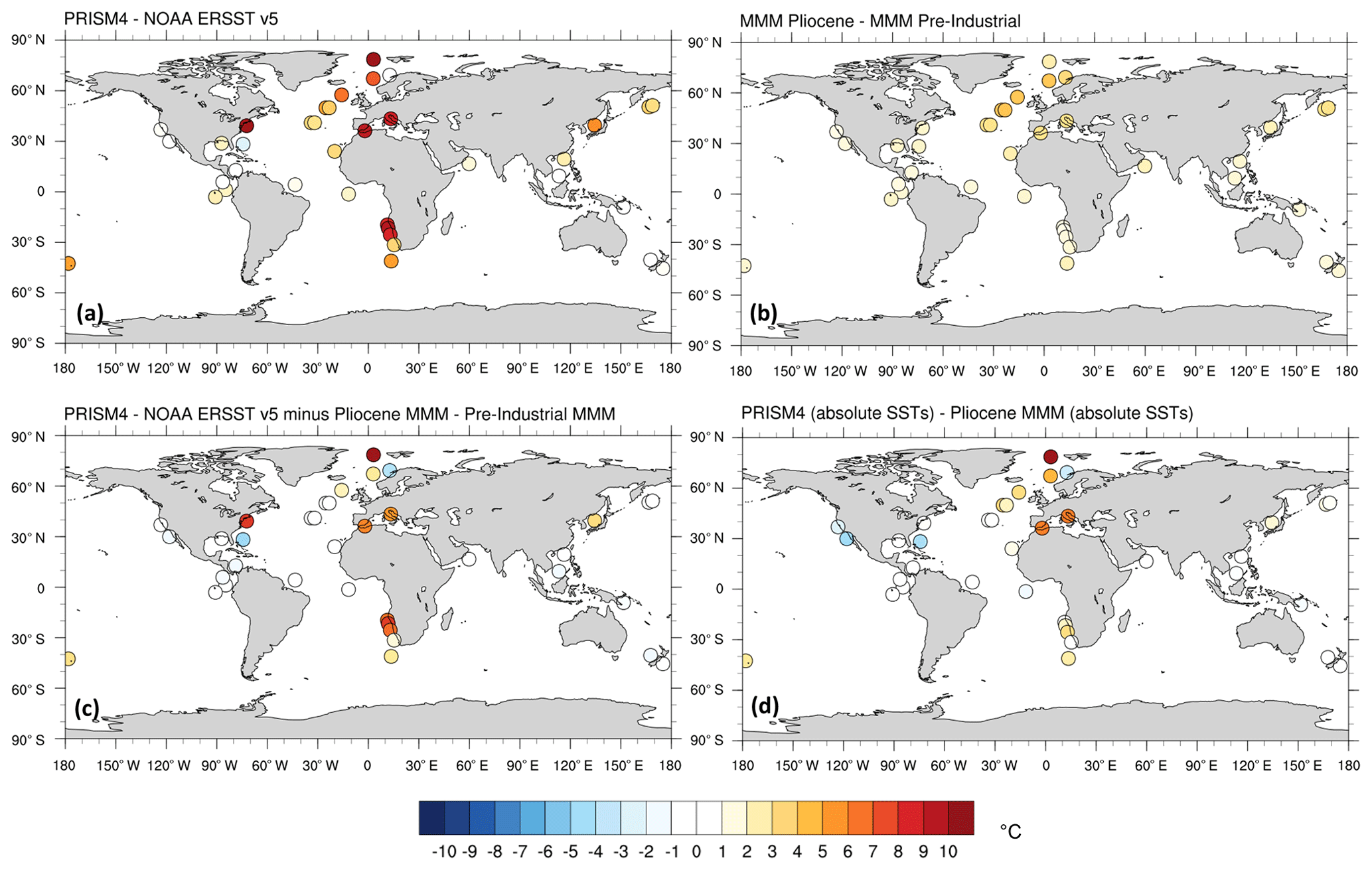
Figure 8(a) PRISM4–NOAA ERSSTv5 SST anomaly for the data points described in Sect. 4. (b) Multi-model mean PlioCore–PICtrl SST anomaly at the points where data are available. (c) The difference between the SST anomaly derived from the data (a) and that of the multi-model mean (b). (d) The PRISM4 SST data minus the PlioCore multi-model mean.
Comparing model-predicted and proxy-based absolute SST estimates for the MIS KM5c time slice (Fig. 8d) yields a similar outcome to the comparison of SST anomalies (Fig. 8c). However, the Benguela region shows greater data–model agreement when considering absolute SSTs than when considering anomalies. Furthermore, a somewhat clearer picture emerges of the model ensemble not producing SSTs that are warm enough in the higher latitudes of the North Atlantic, in the position of the modern North Atlantic gyre and especially in the Nordic Sea, although this appears site dependant as the ensemble overestimates absolute SSTs near Scandinavia.
The proxy data ΔSST minus the mean ΔSST for individual models is shown in Fig. S6. In regions where there was a strong discrepancy between the proxy data ΔSST and the multi-model mean ΔSST, none of the individual models show good data–model agreement. The EC-Earth3.3 model shows an improved agreement with the data in the Mediterranean, the Benguela upwelling system, the site along the east coast of North America and the site to the west of Svalbard. However, this improved data–model agreement is at the expense of reduced data–model agreement elsewhere; many of the low- and middle-latitude sites which had good data–model agreement for the multi-model mean have reduced data–model agreement in EC-Earth3.3. Other models which showed great warming in PlioMIP2 (i.e. CESM2 and CCSM4-Utr) also show a larger ΔSST than the data for some of the tropical- and middle-latitude sites which were in good agreement with the multi-model mean. Models that were less sensitive to Pliocene boundary conditions (i.e. GISS2.1G and NorESM-L) do not predict the amount of warming seen in the data for some of the North Atlantic sites, and the multi-model means performs better. Table 3 shows statistics for the data–model comparison for both individual models and the multi-model mean. The root mean square error (RMSE) between the model and the data is 3.72 for the multi-model mean but is lower in some individual models (namely CESM2, IPSLCM6A, EC-Earth3.3, CESM1.2 and CCSM4-UoT). In general, those models that have a lower data–model RMSE are those which have a higher ECS and a higher PlioCore–PICtrl warming, while less sensitive models have a higher model data RMSE. The average difference between the data and model across all the data points shows a similar pattern. The proxy data are on average 1.5 ∘C warmer than the multi-model mean. However, some individual models have a much smaller average data–model discrepancy (e.g. ∘C). The models with a lower data–model discrepancy are those which also have a lower data–model RMSE and have higher than average PlioCore–PICtl warming.
Table 3Statistical relationships between the proxy data ΔSST and the model ΔSST at each of the individual grid points. The average difference is calculated as , where n is the number of sites.
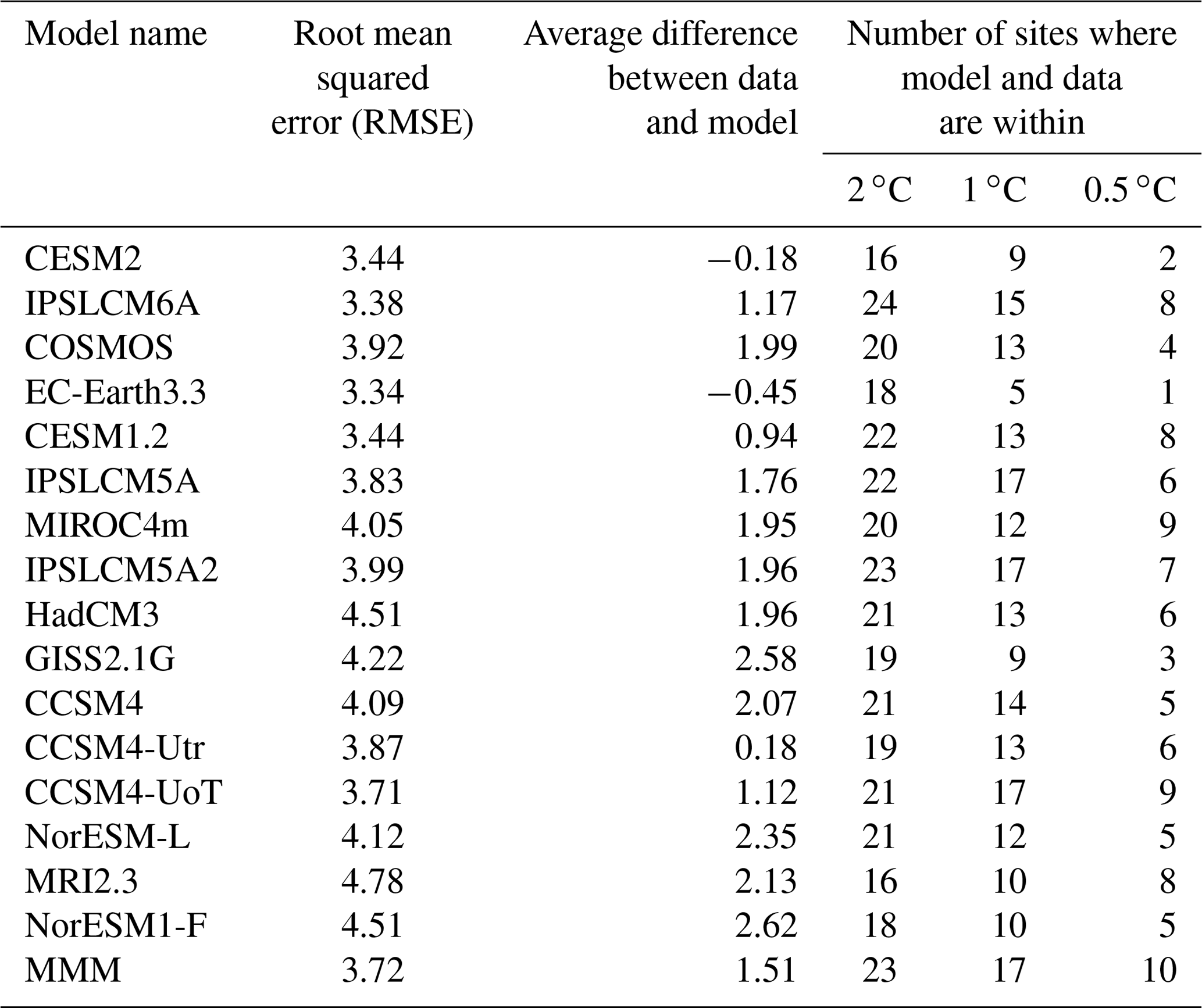
This initial analysis suggests that the most sensitive models agree better with the proxy data than the less sensitive models. However, further analysis does not fully support this result. If we consider how many of the 37 sites have “good” data–model agreement, a different picture emerges. Table 3 shows how many sites have model ΔSST within 2, 1 and 0.5 ∘C of the data ΔSST. Using these diagnostics, the multi-model mean (MMM) performs better than any of the 16 individual models. Those models which have the lowest RMSE and the best average data–model agreement are not those models which have the largest number of sites where model and data agree. For example, CESM2 and EC-Earth3.3 have a particularly low number of sites with good data–model agreement. The models with the highest number of sites with data–model agreements (e.g. ISPLCM6A, CCSM4-UoT, MIROC4m and CESM1.2) show a PlioCore–PICtl warming that is closer to the MMM. The fact that the MMM has more sites with “good” data–model agreement than any individual model highlights the benefit of performing a large multi-model ensemble as we have done for PlioMIP2. It allows inherent biases within individual models to cancel out and likely provides a more accurate way of estimating climate anomalies than can be done with a single model.
Models show a strong relationship between SST anomalies and global mean SAT anomalies (Fig. S7a; , Rsq=0.97) and also a strong correlation between SST averaged over 60∘ N–60∘ S and global mean SAT anomalies (Fig. S7b; , Rsq=0.97). This strong correlation suggests that proxy-based SST anomaly estimates can be used to infer global mean SAT anomalies provided that enough SST proxy data are available to reliably estimate SST anomalies. The multi-model median ratio of ΔSAT∕ΔSST is 1.4, while the multi-model median ratio of ΔSST to ΔSST (60∘ N–60∘ S) is 1.5.
5.1 Large-scale features of a warmer climate (palaeo versus future, older versus younger models)
The range in the global annual mean ΔSAT shown by the PlioMIP2 ensemble (from 1.7 to 5.2 ∘C) is akin to the best estimate (and uncertainty bounds) of predicted global temperature change by 2100 CE using the RCP4.5 (Representative Concentration Pathway) to 8.5 scenarios ( ∘C and ∘C; IPCC, 2013; Table 12.2). Comparing the degree of Pliocene temperature change to predicted changes at 2300 CE, the multi-model mean SAT change is between RCP4.5 (2.5±0.6 ∘C) and RCP6.0 (4.2±1.0 ∘C).
Studies have suggested that the Arctic temperature response to a doubling of atmospheric CO2 concentration may be 1–3 times that of the global annual mean temperature response (Hind et al., 2016). All 16 models within the PlioMIP2 ensemble simulate a polar amplification factor (PA; averaged over the NH and SH) between 2 and 3 (meaning that the high-latitude temperature increase is 2–3 times the global mean temperature increase); however, two models (GISS2.1G and NorESM-L) show PA>3 in the SH. An important caveat to note in the comparison between Pliocene and future predicted polar amplification factors is the major changes in the size of the ice sheets, which in terms of area-of-ice difference affect the SH far more than the NH.
Both model simulations and observations (Byrne and O'Gorman, 2013) show that as temperatures rise, the land warms more than the oceans. This is due to differential lapse rates linked to moisture availability on land. From a theoretical standpoint, the difference in land–sea warming is expected to be monotonic with increases in temperature. However, in reality the rise is non-monotonic and is regulated by latitudinal and regional variations in the availability of soil moisture that influences lapse rates (Byrne and O'Gorman, 2013). This is evident in the PlioMIP2 ensemble with the land–sea amplification of warming noted more strongly in the global mean than in the tropics where precipitation is most abundant (Fig. 3b). For perturbations to the pre-industrial era, modelling and observational studies have shown that land warms 30 % to 70 % more than the oceans (Lambert and Webb, 2011). The PlioMIP2 ensemble broadly supports this conclusion and previous work. It also supports studies that have indicated that the land–sea warming contrast is not dependent upon whether we are considering a transient (RCP-like) or an equilibrium-type climate change scenario (e.g. Lambert and Webb, 2011).
In predictions of future climate change, a consistent result from models is that the warming signal is amplified in the Northern compared to Southern Hemisphere in the extratropics. There have been several studies which have proposed mechanisms to explain this, including heat uptake by the Southern Ocean (Stouffer et al., 1989), as well as ocean heat transport mechanisms (Russell et al., 2006). Within the PlioMIP2 ensemble, 11 out of 16 models show a larger temperature change in the NH extratropics than the SH extratropics (Fig. 3c). This can in part be explained by the area of land in the NH being larger than in the SH and the already discussed amplification of warming over the land versus the oceans. However, the degree of difference is highly model dependent and not as large as has been reported for simulations of future climate change by the Intergovernmental Panel on Climate Change (IPCC, 2013). This may be linked to the intrinsic difference in response between a RCP-like transient and equilibrium climate experiment and in the Pliocene's substantially reduced ice sheets in Antarctica, which are not specified in future climate change simulations. Hence, the noted hemispheric difference in warming for the future may simply be a transient feature that would not be sustained as the ice sheets in Antarctica respond to the warming over centennial to millennial timescales.
The 3.2 ∘C increase in multi-model mean temperature is associated with a 7 % increase in global annual mean precipitation. According to the Clausius–Clapeyron equation, the water holding capacity of the atmosphere increases by about 7 % for each 1 ∘C of temperature increase. The increase in precipitation is therefore less than would be expected if it were assumed that all aspects of the hydrological cycle remained the same as in the pre-industrial era. This is in line with model simulations of future climate change linked to greater temperatures enhancing evaporation from the surface and the atmosphere having a greater moisture carrying capacity but sluggish moisture convection (Held and Soden, 2006).
A particularly robust feature across the ensemble is an increase in precipitation over the modern Sahara Desert and over the Asian monsoon region (Fig. 5d). These regions also experience enhanced precipitation under the RCP8.5 scenario for 2100 (IPCC, 2013, and Fig. SPM.8 therein). However, in other tropical and subtropical regions, the PlioCore model response is small compared to the pre-industrial inter-model standard deviation.
Corvec and Fletcher (2017) showed that in PlioMIP1 studies, the tropical overturning circulations in the MP were weaker than pre-industrial simulations, while Sun et al. (2013) showed that both Hadley cells expanded polewards, a result consistent with (but weaker than) the RCP4.5 scenario. These changes in circulation are consistent with the expansion of the subtropical highs and the corresponding reduction in subtropical oceanic precipitation seen in Fig. 5 for the PlioCore ensemble and in the IPCC (2013; Fig. 7) for RCP scenarios at year 2100.
Although there are many similarities in tropical atmospheric circulation response between Pliocene experiments and the RCP future climate change experiments, there are specific differences mainly relating to (a) the ice sheet changes and their effects on the Equator-to-pole temperature gradient during the Pliocene vis-à-vis the future and (b) the fixed versus transient GHG changes. Nonetheless, the similarities between the general features of the Pliocene experiments and future experiments continue to support the use of the Pliocene as one of the best geological analogues for the near future (Burke et al., 2018) despite the different boundary conditions.
It has been seen that some of the main differences between the PlioMIP1 and PlioMIP2 ensembles are due to the inclusion of new models in PlioMIP2 that were not available at the time of PlioMIP1. This suggests that recent developments in model physics lead to altered responses to Pliocene boundary conditions. For example, PlioMIP2 includes three IPSL models, IPSLCM5A (ΔSAT=2.3 ∘C), IPSLCM5A2 (ΔSAT=2.2 ∘C) and IPSLCM6A (ΔSAT=3.4 ∘C), while only IPSLCM5A contributed to PlioMIP1. PlioMIP2 includes three models from NCAR, CCSM4 (ΔSAT=2.6 ∘C), CESM1.2 (ΔSAT=4.0 ∘C) and CESM2 (ΔSAT=5.2 ∘C), while only CCSM4 contributed to PlioMIP1. Within both these model families, the newer versions provide a greater response to the Pliocene boundary conditions and also have a higher published climate sensitivity.
Across the ensemble there is a significant correlation between sensitivity and model resolution (Fig. S8) with a larger temperature anomaly and precipitation anomaly predicted in higher-resolution models (p<0.05). This suggests that low-resolution models may not be able to capture the full extent of climate change shown by higher-resolution models. However, it is noted that these relationships are only statistical correlations and some models do not show the same pattern. For example, the CCSM4-Utr model has much greater temperature and precipitation anomalies, and CCSM4 has lower temperature and precipitation anomalies than other models of a similar resolution.
5.2 Model representations of Pliocene climate vis-à-vis proxy data
One of the most fundamental changes in experimental design between PlioMIP2/PRISM4 and PlioMIP1/PRISM3D was the approach towards geological data synthesis for data–model comparison, in particular moving from SST and vegetation estimates for a broad time slab to a short SST time series encompassing the MIS KM5c time slice. This was necessary in order to assess to what degree climate variability within the Pliocene could affect the outcomes of data–model comparisons and, fundamentally, to derive greater confidence in the outcomes which could be derived from Pliocene data–model comparisons (Haywood et al., 2013a, b). In addition, PlioMIP2 contains many new models not used in PlioMIP1, and the PlioMIP2 boundary conditions have changed compared to PlioMIP1 (particularly the land–sea mask and the topography). Nevertheless, what emerges from the comparison of the PlioMIP2 SST ensemble to the F&D19_30 SST dataset is a nuanced picture of widespread data–model agreement with specific areas of concern.
Data model comparisons undertaken for PlioMIP1 indicated that the PlioMIP1 ensemble overestimated the amount of SST change as a zonal mean in the tropics (Dowsett et al., 2012, 2013; Fedorov et al., 2013). In PlioMIP2 point-based comparisons, there is little indication of a systematic mismatch between the data and the models. Models and proxy data appear to be broadly consistent in the tropics. The F&D19_30 dataset is comprised of alkenone-based SSTs. In contrast, the PRISM3D dataset used for DMC in PlioMIP1 was time averaged and composed of estimates from a combination of faunal analysis, Mg∕Ca and alkenone-based SSTs. Tierney et al. (2019) demonstrated that the PlioMIP1 ensemble compared well to alkenone-based SST estimates in the tropical Pacific for the whole mid-Pliocene Warm Period, not just the PlioMIP2 time slice, when the alkenone-based temperatures were recalculated using the BAYSPLINE calibration. Therefore, the choice of proxy and inter-proxy calibration alone can be enough to alter the interpretation of the extent to which the model and data agree. In addition, comparing the PlioMIP2 results to an additional dataset of published SSTs for the time slice (McClymont et al., 2020), we see that the first order outcome of data–model comparison is the same as that shown by the comparison to F&D19_30.
The Pliocene minus pre-industrial SST anomaly will not only depend on which SST dataset is chosen to represent the Pliocene but also on the choice of observed SST dataset used for the pre-industrial era. Figure S9 shows the proxy-data-reconstructed SST change using the F&D19_30 dataset but using two different observed datasets for pre-industrial SSTs to create the required proxy data SST anomaly. Using the recently released NOAA ERSST V5 dataset (Huang et al., 2017) to create the anomaly instead of the older HadISST data (Rayner et al., 2003) leads to three sites in the North Atlantic showing a much reduced Pliocene warming. It also means that several sites in the tropics now show a small (2 to 3 ∘C) warming during the Pliocene, while using HadISST data led to an absence of SST warming at these locations. The difference between using NOAA ERSST V5 and HadISST is sufficiently large that it can determine whether the PlioMIP2 ensemble is able to largely match (or mismatch) the proxy-reconstructed temperatures.
Another region of data–model mismatch noted in PlioMIP1 was the North Atlantic Ocean (NA). Haywood et al. (2013a) noted a difference in the model-predicted (multi-model mean) versus proxy-reconstructed (PRISM3D) warming signal of between 2 to 7 ∘C in the NA. The PlioMIP2 multi-model mean SST anomaly appears to be broadly consistent with the F&D19_30 dataset with an SST anomaly at two sites matching to within 1 ∘C and the other to within 3 ∘C (Fig. 8). There are several possible ways to account for this apparent improvement. Firstly, the total number of sites in the NA in F&D19_30 is reduced compared to the PRISM3D SST dataset (Dowsett et al., 2010). The site that led to the 7 ∘C difference noted in Haywood et al. (2013a) is not present in the F&D19_30 dataset. Secondly, the PlioMIP2 experimental design specified both the Canadian Archipelago and Bering Strait as closed. Otto-Bliesner et al. (2017) performed a series of sensitivity tests based on the NCAR CCSM4 PlioMIP1 experiment and found that the closure of these Arctic gateways strengthened the AMOC by inhibiting transport of less saline waters from the Pacific to the Arctic Ocean and from the Arctic Ocean to the Labrador Sea, leading to the warming of NA SSTs. Dowsett et al. (2019) also demonstrated an improved consistency between the proxy-based SST changes and model-predicted SST changes after closing these Arctic gateways in models. It is therefore likely that the multi-model mean SST change in the NA in PlioMIP2 has been influenced by the specified change in Arctic gateways leading to a regionally enhanced fit with proxy data. However, the question regarding the veracity of the specified changes in Arctic gateways in the PRISM4 reconstruction, given the uncertainty and lack of geological evidence either way, remains open and requires further study.
One of the clearest data–model inconsistencies occurs in the Benguela upwelling system, where proxy data indicate more SST warming than the multi-model mean. The simulation of upwelling systems is particularly challenging for global numerical climate models due to the spatial scale of the physical processes involved and the capability of models to represent changes in the structure of the water column (thermocline depth), as well as cloud–surface temperature feedbacks. Dowsett et al. (2013) noted SST discrepancies between the PRISM3D SST reconstruction and the PlioMIP1 ensemble. Their analysis of the seasonal vertical temperature profiles from PlioMIP1 for the Peru upwelling region indicated that models produced a simple temperature offset between PI and the Pliocene but did not simulate any change to thermocline depth.
An assumption that proxy data truly reflect mean annual SSTs in upwelling regions is also worthy of consideration. In upwelling zones, nutrients (and relatively cold waters) are brought to the surface increasing productivity. The upwelling of nutrient rich waters is often seasonally modulated, which could conceivably bias alkenone-based SSTs to the seasonal maximum for nutrient supply and therefore coccolithophore productivity and/or alkenone flux. In the modern ocean, across the most intense region of Benguela upwelling, the productivity seems to be year-round, whereas southern Benguela has the highest productivity during the summer (Rosell-Melé and Prahl, 2013). Ismail et al. (2015), based on observational data, demonstrated that it was surface heating, not vertical mixing related to upwelling, which controls the upper ocean temperature gradient in the region today. This lends some credence to the idea that the observed mismatch between PlioMIP2 ΔSST and the F&D19_30 proxy-based anomaly could arise from the complexities and/or uncertainties associated with interpreting alkenone-based SSTs in the region as simply an indication of mean annual SST (Leduc et al., 2014). However, we note that no seasonal bias has been identified in the modern dataset in the Benguela region (Tierney and Tingley, 2018).
5.3 Equilibrium climate sensitivity, Earth system sensitivity and Pliocene climate
From the analysis shown in Sect. 3.6, a strong relationship between ECS and the ensemble-simulated Pliocene temperature anomaly is discernible. This point is true for the globally averaged temperature anomaly, latitudinal average temperature anomalies in the tropics and specific grid-box-based temperature anomalies over large portions of the globe. Across the ensemble, the tropical Pliocene temperature anomaly is more strongly related to ECS than other latitudes, both as a latitudinal mean and when considering individual grid points. On a grid point by grid point basis, the tropical oceans are strongly related to modelled ECS, suggesting that SST data from the Pliocene tropics have the potential to constrain model estimates of ECS, which highlights the benefits for deriving estimates of ECS from a concentrated effort to reconstruct tropical SST response using the geological record.
For PlioMIP1, Hargreaves and Annan (2016) also found that modelled PlioCore–PICrtl SST anomalies over the tropics (30∘ N–30∘ S) were correlated with modelled ECS, according to
where α and C are constants and ε represents all errors in the regression equation. They then used Eq. (2) along with tropical SST data from PRISM3D (an interpolated dataset of Pliocene proxy SST) to provide a Pliocene-data-constrained estimate of ECS of 1.9–3.7 ∘C. In order to constrain ECS from the data and modelling used in PlioMIP2, we slightly amend the Hargreaves and Annan (2016) methodology because PlioMIP2 proxy data are more sparsely distributed than PlioMIP1 proxy data, and we cannot obtain a reliable estimate of tropical average SST from the data available. To estimate ECS for PlioMIP2, we instead rely on point-based observations (Fig. 8a) and local regressions between PlioCore–PICrtl SST and modelled ECS (Fig. 7c). Hence, we apply Eq. (2) with ΔSST from individual data sites, and α and C will now be location dependent. Using this altered methodology, a different estimate of ECS is obtained for each data point; these estimates are shown in Fig. 9 and have a range of 2.6–4.8 ∘C with a mean ECS of 3.6 ∘C and a standard deviation of 0.6 ∘C. Figure 9 does not imply that ECS is different for each location; instead each value in Fig. 9 is an estimate of ECS and incorporates the true Pliocene-constrained ECS along with several errors. For a data point to be included in Fig. 9, we required that two conditions were met. Firstly, we required that the relationship between local PlioCore–PICrtl and a model's ECS was significant at the 95 % confidence level (p<0.05; these regions are hatched in Fig. 7d). Secondly, we required that at least one of the models in the PlioMIP2 ensemble was within 1 ∘C of the data; this second condition meant that we excluded two sites off the eastern United States, two sites from the Mediterranean and two sites from Benguela – despite these sites showing a theoretical relationship between PlioCore–PICrtl and ECS. Altogether 13 data points fulfilled both these conditions and could be used to estimate ECS. The range of estimates of ECS from PlioMIP2 (2.6–4.8 ∘C) are similar to IPCC (1.5–4.5 ∘C) but are slightly higher than was estimated from PlioMIP1 (1.9–3.7 ∘C). It is not currently possible to add reliable error bars to the range of ECS estimates from PlioMIP2. However, as the Tier1 PlioMIP2 experiments with CO2 set to 350 and 450 ppmv become available, we will be able to provide an indication as to how uncertainties in the KM5c CO2 would affect the PlioMIP2/PRISM4-constrained estimates of ECS. In addition, as more orbitally tuned SST data become available, it will be necessary to revisit the ECS analysis in order to ensure maximum accuracy.
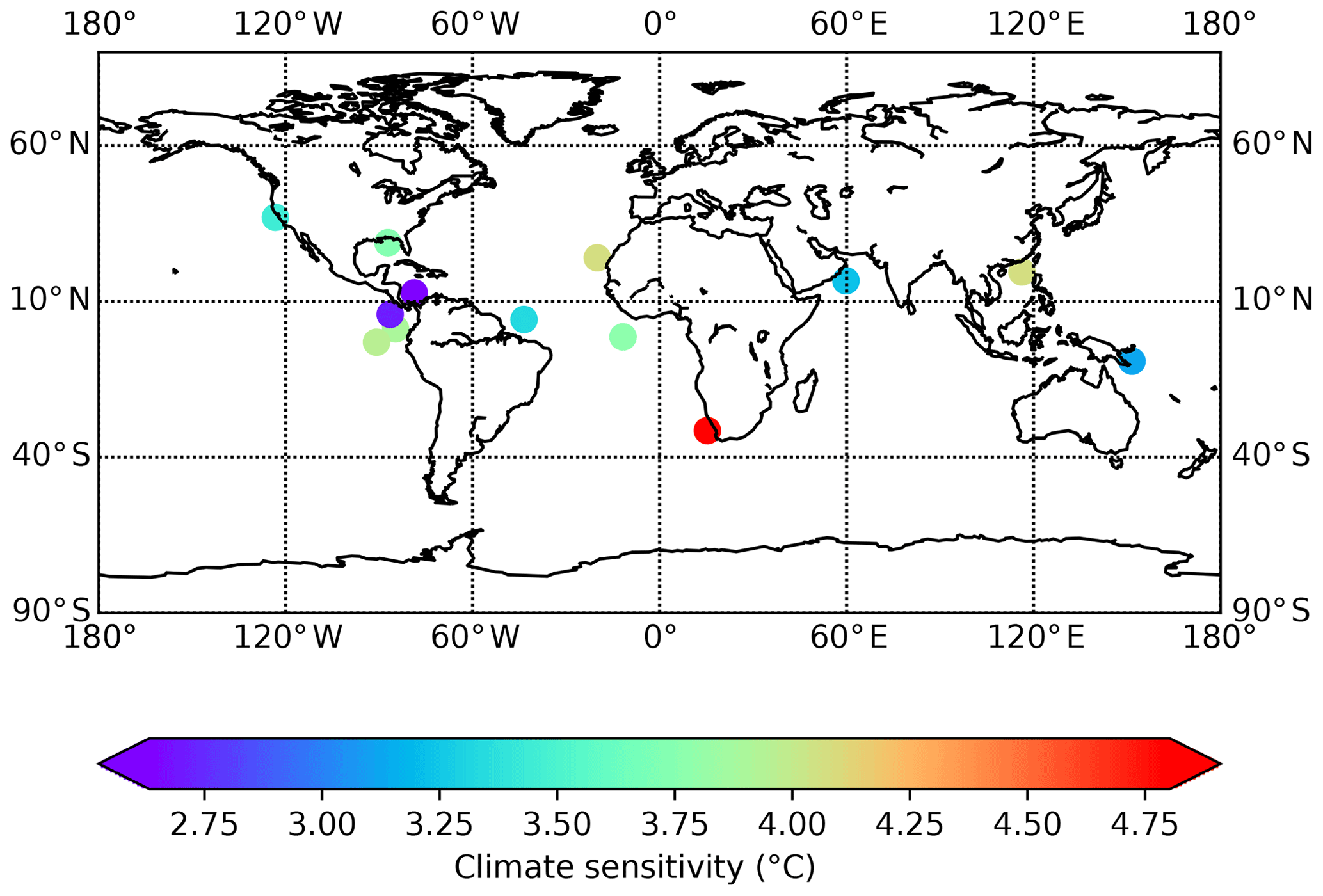
Figure 9Equilibrium climate sensitivity estimated from the data shown in Fig. 8 based on the modelled grid-point-based regressions between PlioCore–PICtrl and ECS. This analysis was limited to those data points which were within 1 ∘C of the range of PlioMIP2 models, and it was also limited to those sites which were in a grid box where the modelling suggested a significant relationship between the PlioCore–PICtrl SAT anomaly and the ECS.
The emergence of the concept of longer-term sensitivity, ESS, can be at least partly attributed to the study of the Pliocene epoch (Lunt et al., 2010; Haywood et al., 2013a). However, as Hunter et al. (2019) state clearly, the comparison between ECS, PlioCore–PICrtl, and ESS can only be robust if an assumption is made that the PlioMIP2 model boundary conditions are a good approximation to the equilibrated Earth system with enhanced atmospheric CO2 concentration. This may appear to be a reasonable assumption now since the changes in non-glacial elements of the PRISM4 palaeogeography are limited. Yet, within the bounds of plausible uncertainty, a larger number of additional palaeogeographic modifications remain possible for the late Pliocene than were incorporated into the PRISM4 reconstruction (see Hill, 2015 and De Schepper et al., 2015) and which may have a bearing on how well the Pliocene is seen to approximate an equilibrated modern Earth system in the years ahead.
PlioMIP1 determined a range in the ESS∕CS ratio of between 1.1 and 2.0 with a best estimate of 1.5. In PlioMIP2, which has benefited from the access to a larger array of models and new boundary conditions, the range and best estimate of the ESS∕CS ratio is similar but slightly larger (1.1 to 2.9 and 1.7 respectively). Therefore, new modelling and new constraints on the data for PlioMIP2 suggest a slight increase in estimates of both the ESS∕CS ratio and data-constrained estimates of ECS between PlioMIP1 and PlioMIP2.
The Pliocene Model Intercomparison Project Phase 2 represents one of the largest ensembles of climate models of different complexities and spatial resolution ever assembled to study a specific interval in Earth history. PlioMIP2 builds on the findings of PlioMIP1 and incorporates state-of-the-art reconstructions of Pliocene boundary conditions and new temporally consistent sea surface temperature proxy data which underpin the new data–model comparison. The major findings of the work include the following.
- -
Global annual mean surface air temperatures increase by 1.7 to 5.2 ∘C compared to the pre-industrial era with a multi-model average increase of 3.2 ∘C.
- -
The mean annual surface air temperature response is larger in PlioMIP2 than in PlioMIP1 mainly due to the addition of new and more sensitive models in PlioMIP2.
- -
The multi-model mean annual total precipitation rate increases by 7 % compared to the pre-industrial era, while the modelled range of precipitation increases by between 2 % and 13 %.
- -
The multi-model mean anomaly between the Pliocene and pre-industrial era is statistically robust for surface air temperature and sea surface temperature over most of the globe. The multi-model mean precipitation anomaly is robust at middle–high latitudes and in monsoon regions but is smaller than the inter-model standard deviation in many parts of the tropics and subtropics.
- -
The degree of polar amplification of surface air temperature change is generally consistent with RCP transient climate modelling experiments used to predict future climate, implying that CO2 changes dominate the ice sheet changes in the PlioCore experiments.
- -
The land warms more than the oceans in a manner akin to future climate change simulations.
- -
As an ensemble, average NH warming does not show a clear seasonal cycle, but a clear seasonal cycle is seen in many individual models.
- -
The difference in the average warming between the hemispheres is subdued relative to simulations of 2100 CE climate. This is likely due to the substantial changes to the albedo feedback mechanism in the Southern Hemisphere following the removal of large areas of the Antarctic ice sheet in the mid-Pliocene.
- -
There is a statistically significant relationship between ECS and Pliocene global annual average temperature change. The PlioMIP2 ensemble finds that ESS is greater than ECS by a best estimate of 67 %.
- -
Model estimates of the relationship between ECS and PlioCore–PICrtl, combined with the PlioMIP2 ΔSST, provide a data-constrained estimate of ECS with a range of 2.6–4.8 ∘C. This is larger than the values suggested from PlioMIP1 (1.9–3.7 ∘C).
- -
The PlioMIP2 model ensemble shows broad agreement on the polar amplification of the global warming signal and tropical enhancement of rainfall anomalies. Inter-model differences in simulated temperature are mostly found in polar regions and where the land–sea mask and orography of Pliocene palaeogeography differ from today.
- -
The PlioMIP2 ensemble appears to be broadly reconcilable with new temporally specific records of sea surface temperatures. Significant agreement between simulated and reconstructed temperature change is seen with notable local signals of data–model disagreement. Differences between observed pre-industrial sea surface temperature datasets are large enough to have a significant impact on how well models reproduce proxy-reconstructed ocean temperature changes.
The data required to produce the results in this paper is available in the Supplement. More complete data for PlioMIP2 (with the exception of IPSLCM6A and GISS2.1G) is available upon request from Alan M. Haywood (a.m.haywood@leeds.ac.uk). PlioMIP2 data from IPSLCM6A and GISS2.1G can be obtained from the Earth System Grid Federation (ESGF) (https://esgf-node.llnl.gov/search/cmip6/, last access: 16 September 2020, ESGF, 2020).
The supplement related to this article is available online at: https://doi.org/10.5194/cp-16-2095-2020-supplement.
AMH, HJD and AMD planned and coordinated PlioMIP2. AMH, JCT and AMD prepared the paper with contributions from all coauthors. HJD and KMF contributed data and advice for the data–model comparison. SJH, WLC, AAO, CS, GL, DC, WRP, NT, CC, GR, XL, ZZ, CG, KHN, QZ, QL, YK, MAC, LES, BLOB, RF, ECB, ASvdH and MLJB provided the PlioMIP2 experiments run with the individual models.
The authors declare that they have no conflict of interest.
This article is part of the special issues “PlioMIP Phase 2: experimental design, implementation and scientific results” and “Paleoclimate Modelling Intercomparison Project phase 4 (PMIP4) (CP/GMD inter-journal SI)”. It is not associated with a conference.
We acknowledge the use of NOAA_ERSST_V5 data provided by the NOAA/OAR/ESRL PSD, Boulder, Colorado, USA, from their website at https://www.esrl.noaa.gov/psd/ (last access: 12 September 2019). Alan M. Haywood, Julia C. Tindall, Aisling M. Dolan, Stephen J. Hunter and Daniel J. Hill acknowledge the FP7 Ideas programme: European Research Council (grant no. PLIO-ESS, 278636), the Past Earth Network (EPSRC grant no. EP/M008.363/1) and the University of Leeds Advanced Research Computing service. Julia C. Tindall was also supported through the Centre for Environmental Modelling and Computation (CEMAC), University of Leeds. Harry J. Dowsett and Kevin M. Foley acknowledge support from the USGS Climate Research and Development Program. This research used samples and/or data provided by the Ocean Drilling Program (ODP) and International Ocean Discovery Program (IODP). Any use of trade, firm, or product names is for descriptive purposes only and does not imply endorsement by the U.S. Government. Bette L. Otto-Bliesner, Esther C. Brady and Ran Feng acknowledge that material for their participation is based upon work supported by the National Center for Atmospheric Research, which is a major facility sponsored by the National Science Foundation (NSF) (cooperative agreement no. 1852977 and NSF OPP grant no. 1418411). The CESM project is supported primarily by the National Science Foundation. Computing and data storage resources, including the Cheyenne supercomputer (https://doi.org/10.5065/D6RX99HX), were provided by the Computational and Information Systems Laboratory (CISL) at NCAR. NCAR is sponsored by the National Science Foundation. Ning Tan, Camille Contoux and Gilles Ramstein were granted access to the HPC resources of TGCC under the allocations 2016-A0030107732, 2017-R0040110492 and 2018-R0040110492 (gencmip6) and 2019-A0050102212 (gen2212) provided by GENCI. The IPSL-CM6 team of the IPSL Climate Modelling Centre (https://cmc.ipsl.fr, last access: 16 September 2020) is acknowledged for having developed, tested, evaluated and tuned the IPSL climate model, as well as performed and published the CMIP6 experiments. Christian Stepanek acknowledges funding from the Helmholtz Climate Initiative REKLIM. Christian Stepanek and Gerrit Lohmann acknowledge funding via the Alfred Wegener Institute's research programme Marine, Coastal and Polar Systems. Qiong Zhang acknowledge support from the Swedish Research Council (2013-06476 and 2017-04232). Simulations with EC-Earth were performed on resources provided by the Swedish National Infrastructure for Computing (SNIC) at the National Supercomputer Centre (NSC). Wing-Le Chan and Ayako Abe-Ouchi acknowledge funding from JSPS (KAKENHI grant no. 17H06104 and MEXT KAKENHI grant no. 17H06323). Their simulations with MIROC4m were performed on the Earth Simulator at JAMSTEC, Yokohama, Japan. The work by Anna S. von der Heydt and Michiel L. J. Baatsen was carried out under the program of the Netherlands Earth System Science Centre (NESSC), financially supported by the Ministry of Education, Culture and Science (OCW grant no. 024.002.001). Simulations with CCSM4-Utr were performed at the SURFsara Dutch national computing facilities and were sponsored by NWO-EW (Netherlands Organisation for Scientific Research, Exact Sciences) (project no. 17189). W. Richard Peltier and Deepak Chandan were supported by Canadian NSERC Discovery Grant A9627, and they wish to acknowledge the support of SciNet HPC Consortium for providing computing facilities. SciNet is funded by the Canada Foundation for Innovation under the auspices of Compute Canada, the Government of Ontario, the Ontario Research Fund – Research Excellence, and the University of Toronto. Xiangyu Li acknowledges financial support from the China Scholarship Council (201804910023) and the China Postdoctoral Science Foundation (project no. 2015M581154). The NorESM simulations benefitted from resources provided by UNINETT Sigma2 – the National Infrastructure for High Performance Computing and Data Storage in Norway. The authors would also like to thank Tim Herbert and an anonymous reviewer for helpful comments on an earlier version of this paper.
This research has been supported by the Past Earth Network (EPSRC grant no. EP/M008.363/1).
This paper was edited by Appy Sluijs and reviewed by Tim Herbert and one anonymous referee.
Balsamo, G., Viterbo, P., Beljaars, A., van den Hurk, B., Hirschi, M., Betts, A. K., and Scipal, K.: A Revised Hydrology for the ECMWF Model: Verification from Field Site to Terrestrial Water Storage and Impact in the Integrated Forecast System, J. Hydrometeorol., 10, 623–643, https://doi.org/10.1175/2008jhm1068.1, 2009.
Balsamo, G., Pappenberger, F., Dutra, E., Viterbo, P., and van der Hurk, B.: A revised land hydrology in the ECMWF model: a step towards daily water flux prediction in a fully-closed water cycle, Hydrol. Process., 25, 1046–1054, https://doi.org/10.1002/hyp.7808, 2011.
Bitz, C. M., Shell, K. M., Gent, P. R., Bailey, D. A., Danabasoglu, G., Armour, K. C., Holland, M. M., and Kiehl, J. T.: Climate Sensitivity of the Community Climate System Model, Version 4, J. Climate, 25, 3053–3070, https://doi.org/10.1175/JCLI-D-11-00290.1, 2012.
Boucher, O., Servonnat, J., Albright, A. L., et al.: Presentation and evaluation of the IPSL‐CM6A‐LR climate model, J. Adv. Model. Earth Sy., 12, e2019MS002010, https://doi.org/10.1029/2019MS002010, 2020.
Burls, N. J. and Fedorov, A. V.: Simulating Pliocene warmth and a permanent El Nino-like state: The role of cloud albedo, Paleoceanography, 29, 893–910, https://doi.org/10.1002/2014pa002644, 2014.
Byrne, M. P. and O'Gorman, P. A.: Land-Ocean Warming Contrast over a Wide Range of Climates: Convective Quasi-Equilibrium Theory and Idealized Simulations, J. Climate, 26, 4000-4016, https://doi.org/10.1175/jcli-d-12-00262.1, 2013.
Cattle, H. and Crossley, J.: Modelling Arctic climate change, Philos. T. Roy. Soc. A, 352, 201–213, https://doi.org/10.1098/rsta.1995.0064, 1995.
Chan, W.-L. and Abe-Ouchi, A.: Pliocene Model Intercomparison Project (PlioMIP2) simulations using the Model for Interdisciplinary Research on Climate (MIROC4m), Clim. Past, 16, 1523–1545, https://doi.org/10.5194/cp-16-1523-2020, 2020.
Chandan, D. and Peltier, W. R.: Regional and global climate for the mid-Pliocene using the University of Toronto version of CCSM4 and PlioMIP2 boundary conditions, Clim. Past, 13, 919–942, https://doi.org/10.5194/cp-13-919-2017, 2017.
Chandan, D. and Peltier, W. R.: On the mechanisms of warming the mid-Pliocene and the inference of a hierarchy of climate sensitivities with relevance to the understanding of climate futures, Clim. Past, 14, 825–856, https://doi.org/10.5194/cp-14-825-2018, 2018.
Chandler, M., Rind, D., and Thompson, R.: Joint investigations of the middle Pliocene climate II: GISS GCM Northern Hemisphere results, Global Planet. Change, 9, 197–219, https://doi.org/10.1016/0921-8181(94)90016-7, 1994.
Corvec, S. and Fletcher, C. G.: Changes to the tropical circulation in the mid-Pliocene and their implications for future climate, Clim. Past, 13, 135–147, https://doi.org/10.5194/cp-13-135-2017, 2017.
Cox, P. M., Betts, R. A., Bunton, C. B., Essery, R. L. H., Rown-tree, P. R., and Smith, J.: The impact of new land surface physics on the GCM simulation of climate and climate sensitivity, Clim. Dynam., 15, 183–203, https://doi.org/10.1007/s003820050276, 1999.
Craig, A. P., Vertenstein, M., and Jacob, R.: A new flexible coupler for earth system modeling developed for CCSM4 and CESM1, Int. J. High Perform. C., 26, 31–42, https://doi.org/10.1177/1094342011428141, 2012.
Danabasoglu, G., Lamarque, J. F., Bacmeister, J., Bailey, D. A., DuVivier, A. K., Edwards, J., Emmons, L. K., Fasullo, J., Garcia, R., Gettelman, A., and Hannay, C.: The community earth system model version 2 (CESM2), J. Adv. Model. Earth Sy., 12, e2019MS001916, https://doi.org/10.1029/2019MS001916, 2020.
De La Vega, E., Chalk, T.B., Foster, G.L., Bysani, R., and Wilson, P.A.: Warming in a warm world: Orbital CO2 forcing variations in the warm Pliocene, in: 2018 AGU Fall Meeting, San Francisco, CA, 11 December 2018, Abstract PP21C-1434, 2018.
de Nooijer, W., Zhang, Q., Li, Q., Zhang, Q., Li, X., Zhang, Z., Guo, C., Nisancioglu, K. H., Haywood, A. M., Tindall, J. C., Hunter, S. J., Dowsett, H. J., Stepanek, C., Lohmann, G., Otto-Bliesner, B. L., Feng, R., Sohl, L. E., Tan, N., Contoux, C., Ramstein, G., Baatsen, M. L. J., von der Heydt, A. S., Chandan, D., Peltier, W. R., Abe-Ouchi, A., Chan, W.-L., Kamae, Y., and Brierley, C. M.: Evaluation of Arctic warming in mid-Pliocene climate simulations, Clim. Past Discuss., https://doi.org/10.5194/cp-2020-64, in review, 2020.
De Schepper, S., Schreck, M., Beck, K. M., Matthiessen, J., Fahl, K., and Mangerud, G.: Early Pliocene onset of modern Nordic Seas circulation related to ocean gateway changes, Nat. Commun., 6, 8659, https://doi.org/10.1038/ncomms9659, 2015.
Dowsett, H. J., Cronin, T. M., Poore, R. Z., Thompson, R. S., Whatley, R. C., and Wood, A. M.: Micropaleontological Evidence for Increased Meridional Heat Transport in the North Atlantic Ocean during the Pliocene, Science, 258, 1133–1135, https://doi.org/10.1126/science.258.5085.1133, 1992.
Dowsett, H., Robinson, M., Haywood, A., Salzmann, U., Hill, D., Sohl, L., Chandler, M., Williams, M., Foley, K., and Stoll, D.: The PRISM3D paleoenvironmental reconstruction, Stratigraphy, 7, 123–139, 2010.
Dowsett, H. J., Robinson, M. M., Haywood, A. M., Hill, D. J., Dolan, A. M., Stoll, D. K., Chan, W. L., Abe-Ouchi, A., Chandler, M. A., Rosenbloom, N. A., Otto-Bliesner, B. L., Bragg, F. J., Lunt, D. J., Foley, K. M., and Riesselman, C. R.: Assessing confidence in Pliocene sea surface temperatures to evaluate predictive models, Nat. Clim. Change, 2, 365–371, https://doi.org/10.1038/nclimate1455, 2012.
Dowsett, H. J., Foley, K. M., Stoll, D.K., Chandler, M.A., Sohl, L.E., Bentsen, M., Otto-Bliesner, B. L., Bragg, F. J., Chan, W.-L., Contoux, C., Dolan, A. M., Haywood, A. M., Jonas, J. A., Jost, A., Kamae, Y., Lohmann, G., Lunt, D. J., Nisancioglu, K. H., Abe-Ouchi, A., Ramstein, G., Riesselman, C. R., Robinson, M. M., Rosenbloom, N. A., Salzmann, U., Stepanek, C., Strother, S. L., Ueda, H., Yan, Q., and Zhang, Z.: Sea Surface Temperature of the mid-Piacenzian Ocean: A Data-Model Comparison, Scientific Reports, 3, 2013, https://doi.org/10.1038/srep02013, 2013.
Dowsett, H., Dolan, A., Rowley, D., Moucha, R., Forte, A. M., Mitrovica, J. X., Pound, M., Salzmann, U., Robinson, M., Chandler, M., Foley, K., and Haywood, A.: The PRISM4 (mid-Piacenzian) paleoenvironmental reconstruction, Clim. Past, 12, 1519–1538, https://doi.org/10.5194/cp-12-1519-2016, 2016.
Dowsett, H. J., Robinson, M. M., Foley, K. M., Herbert, T. D., Otto-Bliesner, B. L., and Spivey, W.: The mid-Piacenzian of the North Atlantic Ocean, Stratigraphy, 16, 119–144, https://doi.org/10.29041/strat.16.3.119-144, 2019.
Dufresne, J. L., Foujols, M. A., Denvil, S., Caubel, A., Marti, O., Aumont, O., Balkanski, Y., Bekki, S., Bellenger, H., Benshila, R., Bony, S., Bopp, L., Braconnot, P., Brockmann, P., Cadule, P., Cheruy, F., Codron, F., Cozic, A., Cugnet, D., Noblet, N., Duvel, J. P., Ethé, C., Fairhead, L., Fichefet, T., Flavoni, S., Friedlingstein, P., Grandpeix, J. Y., Guez, L., Guilyardi, E., Hauglustaine, D., Hourdin, F., Idelkadi, A., Ghattas, J., Joussaume, S., Kageyama, M., Krinner, G., Labetoulle, S., Lahellec, A., Lefebvre, M.P., Lefevre, F., Levy, C., Li, Z. X., Lloyd, J., Lott, F., Madec, G., Mancip, M., Marchand, M., Masson, S., Meurdesoif, Y., Mignot, J., Musat, I., Parouty, S., Polcher, J., Rio, C., Schulz, M., Swingedouw, D., Szopa, S., Talandier, C., Terray, P., Viovy, N., and Vuichard, N.: Climate change projections using the IPSL-CM5 Earth System Model: from CMIP3 to CMIP5, Clim. Dynam., 40, 2123–2165, https://doi.org/10.1007/s00382-012-1636-1, 2013.
ESGF: WCRP Coupled Model Intercomparison Project (Phase 6), available at: https://esgf-node.llnl.gov/search/cmip6/, last access: 16 September 2020.
Feng, R., Otto-Bliesner, B. L., Xu, Y. Y., Brad, E., Fletcher, T., and Ballantyne, A.: Contributions of aerosol-cloud interactions to mid-Piacenzian seasonally sea ice-free Arctic Ocean, Geophys. Res. Lett., 46, 9920–9929, https://doi.org/10.1029/2019GL083960, 2019.
Feng, R., Otto-Bliesner, B. L, Brady, E. C., and Rosenbloom, N. A.: Increasing Earth System Sensitivity in mid-Pliocene simulations from CCSM4 to CESM2, J. Adv. Model. Earth Sy., https://doi.org/10.1002/essoar.10501546.1, online first, 2020.
Fedorov, A. V., Brierley, C. M., and Emanuel, K.: Tropical cyclones and permanent El Niño in the early Pliocene epoch, Nature, 463, 1066–1070, https://doi.org/10.1038/nature08831, 2010.
Fedorov, A. V., Brierley, C. M., Lawrence, K. T., Liu, Z., Dekens, P. S., and Ravelo, A. C.: Patterns and mechanisms of early Pliocene warmth, Nature, 496, 43–49, https://doi.org/10.1038/nature12003, 2013.
Fichefet, T. and Maqueda, M. A. M.: Sensitivity of a global sea ice model to the treatment of ice thermodynamics and dynamics, J. Geophys. Res., 102, 12609–12646, https://doi.org/10.1029/97JC00480, 1997.
Fichefet, T. and Maqueda, M. A. M.: Modelling the influence of snow accumulation and snow-ice formation on the seasonal cycle of the Antarctic sea-ice cover, Clim. Dynam., 15, 251–268, https://doi.org/10.1007/s003820050280, 1999.
Foley, K. M. and Dowsett, H. J.: Community sourced mid-Piacenzian sea surface temperature (SST) data, US Geological Survey data release, https://doi.org/10.5066/P9YP3DTV, 2019.
Gent, P. R., Danabasoglu, G., Donner, L. J., Holland, M. M., Hunke, E. C., Jayne, S. R., Lawrence, D. M., Neale, R. B., Rasch, P. J., Vertenstein, M., and Worley, P. H.: The community climate system model version 4, J. Climate, 24, 4973–4991, https://doi.org/10.1175/2011JCLI4083.1, 2011.
Gettelman, A., Hannay, C., Bacmeister, J. T., Neale, R. B., Pendergrass, A. G., Danabasoglu, G., Lamarque, J. F., Fasullo, J. T., Bailey, D. A., Lawrence, D. M., and Mills, M. J.: High climate sensitivity in the Community Earth System Model Version 2 (CESM2), Geophys. Res. Lett., 46, 8329–8337, 2019.
Gettelman, A., Kay, J. E., and Shell, K. M.: The Evolution of Climate Sensitivity and Climate Feedbacks in the Community Atmosphere Model, J. Climate, 25, 1453–1469, https://doi.org/10.1175/JCLI-D-11-00197.1, 2012.
Gordon, C., Cooper, C., Senior, C. A., Banks, H., Gregory, J. M., Johns, T. C., Mitchell, J. F. B., and Wood, R. A.: The simulation of SST, sea ice extents and ocean heat transports in a version of the Hadley Centre coupled model without flux adjustments, Clim. Dynam., 16, 147–168, https://doi.org/10.1007/s003820050010, 2000.
Guo, C., Bentsen, M., Bethke, I., Ilicak, M., Tjiputra, J., Toniazzo, T., Schwinger, J., and Otterå, O. H.: Description and evaluation of NorESM1-F: a fast version of the Norwegian Earth System Model (NorESM), Geosci. Model Dev., 12, 343–362, https://doi.org/10.5194/gmd-12-343-2019, 2019.
Hagemann, S. and Gates, L. D.: Improving a subgrid runoff parameterization scheme for climate models by the use of high-resolution data derived from satellite observations, Clim. Dynam., 21, 349–359, https://doi.org/10.1007/s00382-003-0349-x, 2003.
Hagemann, S. and Dumenil, L.: A parametrization of the lateral waterflow for the global scale, Clim. Dynam., 14, 17–31, https://doi.org/10.1007/s003820050205, 1998.
Hargreaves, J. C. and Annan, J. D.: Could the Pliocene constrain the equilibrium climate sensitivity?, Clim. Past, 12, 1591–1599, https://doi.org/10.5194/cp-12-1591-2016, 2016.
Haywood, A. M. and Valdes, P. J.: Modelling Pliocene warmth: contribution of atmosphere, oceans and cryosphere, Earth Planet. Sc. Lett., 218, 363–377, https://doi.org/10.1016/S0012-821X(03)00685-X, 2004.
Haywood, A. M., Valdes, P. J., and Sellwood, B. W.: Global scale palaeoclimate reconstruction of the middle Pliocene climate using the UKMO GCM: initial results, Global Planet. Change, 25, 239–256, https://doi.org/10.1016/S0921-8181(00)00028-X, 2000.
Haywood, A. M., Dowsett, H. J., Otto-Bliesner, B., Chandler, M. A., Dolan, A. M., Hill, D. J., Lunt, D. J., Robinson, M. M., Rosenbloom, N., Salzmann, U., and Sohl, L. E.: Pliocene Model Intercomparison Project (PlioMIP): experimental design and boundary conditions (Experiment 1), Geosci. Model Dev., 3, 227–242, https://doi.org/10.5194/gmd-3-227-2010, 2010.
Haywood, A. M., Dowsett, H. J., Robinson, M. M., Stoll, D. K., Dolan, A. M., Lunt, D. J., Otto-Bliesner, B., and Chandler, M. A.: Pliocene Model Intercomparison Project (PlioMIP): experimental design and boundary conditions (Experiment 2), Geosci. Model Dev., 4, 571–577, https://doi.org/10.5194/gmd-4-571-2011, 2011.
Haywood, A. M., Hill, D. J., Dolan, A. M., Otto-Bliesner, B. L., Bragg, F., Chan, W.-L., Chandler, M. A., Contoux, C., Dowsett, H. J., Jost, A., Kamae, Y., Lohmann, G., Lunt, D. J., Abe-Ouchi, A., Pickering, S. J., Ramstein, G., Rosenbloom, N. A., Salzmann, U., Sohl, L., Stepanek, C., Ueda, H., Yan, Q., and Zhang, Z.: Large-scale features of Pliocene climate: results from the Pliocene Model Intercomparison Project, Clim. Past, 9, 191–209, https://doi.org/10.5194/cp-9-191-2013, 2013a.
Haywood, A. M., Dolan, A. M., Pickering, S. J., Dowsett, H. J., McClymont, E. L., Prescott, C. L., Salzmann, U., Hill, D. J., Hunter, S. J., Lunt, D. J., Pope, J. O., and Valdes, P. J.: On the identification of a Pliocene time slice for data-model comparison, Philos. T. Roy. Soc. A, 371, 20120515, https://doi.org/10.1098/rsta.2012.0515, 2013b.
Haywood, A. M., Dowsett, H. J., Dolan, A. M., Rowley, D., Abe-Ouchi, A., Otto-Bliesner, B., Chandler, M. A., Hunter, S. J., Lunt, D. J., Pound, M., and Salzmann, U.: The Pliocene Model Intercomparison Project (PlioMIP) Phase 2: scientific objectives and experimental design, Clim. Past, 12, 663–675, https://doi.org/10.5194/cp-12-663-2016, 2016a.
Haywood, A. M., Dolan, A., and Chan, W.-L. (Eds.): PlioMIP Phase 2: experimental design, implementation and scientific results, Clim. Past, https://cp.copernicus.org/articles/special_issue642.html (last access: last access: 16 September 2020), 2016b.
Hazeleger, W., Wang, X., Severijns, C., Stefanescu, S., Bintanja, R., Sterl, A., Wyser, K., Semmler, T., Yang, S., van den Hurk, B., van Noije, T., van der Linden, E., and van der Wiel, K.: EC-Earth V2.2: description and validation of a new seamless earth system prediction model, Clim. Dynam., 39, 2611–2629, https://doi.org/10.1007/s00382-011-1228-5, 2012.
Held, I. M. and Soden, B. J.: Robust responses of the hydrological cycle to global warming, J. Climate, 19, 5686–5699, https://doi.org/10.1175/JCLI3990.1, 2006.
Hill, D. J.: The non-analogue nature of Pliocene temperature gradients, Earth Planet. Sc. Lett., 425, 232–241, https://doi.org/10.1016/j.epsl.2015.05.044, 2015.
Hill, D. J., Haywood, A. M., Lunt, D. J., Hunter, S. J., Bragg, F. J., Contoux, C., Stepanek, C., Sohl, L., Rosenbloom, N. A., Chan, W.-L., Kamae, Y., Zhang, Z., Abe-Ouchi, A., Chandler, M. A., Jost, A., Lohmann, G., Otto-Bliesner, B. L., Ramstein, G., and Ueda, H.: Evaluating the dominant components of warming in Pliocene climate simulations, Clim. Past, 10, 79–90, https://doi.org/10.5194/cp-10-79-2014, 2014.
Hind, A., Zhang, Q., and Brattstrom, G.: Problems encountered when defining Arctic amplification as a ratio, Scientific Reports, 6, 30469, https://doi.org/10.1038/srep30469, 2016.
Holland, M. M., Bailey, D. A., Briegleb, B. P., Light, B., and Hunke, E.: Improved Sea Ice Shortwave Radiation Physics in CCSM4: The Impact of Melt Ponds and Aerosols on Arctic Sea Ice, J. Climate, 25, 1413–1430, https://doi.org/10.1175/JCLI-D-11-00078.1, 2012.
Hourdin, F., Musat, I., Bony, S., Braconnot, P., Codron, F., Dufresne, J. L., Fairhead, L., Filiberti, M. A., Friedlingstein, P., Grandpeix, J. Y., Krinner, G., Levan, P., Li, Z. X., and Lott, F.: The LMDZ4 general circulation model: climate performance and sensitivity to parametrized physics with emphasis on tropical convection, Clim. Dynam., 27, 787–813, https://doi.org/10.1007/s00382-006-0158-0, 2006.
Hourdin, F., Grandpeix, J. Y., Rio, C., Bony, S., Jam, A., Cheruy, F., Rochetin, N., Fairhead, L., Idelkadi, A., Musat, I., Dufresne, J. L., Lahellec, A., Lefebvre, M. P., and Roehrig, R.: LMDZ5B: the atmospheric component of the IPSL climate model with revisited parameterizations for clouds and convection, Clim. Dynam., 40, 2193–2222, https://doi.org/10.1007/s00382-012-1343-y, 2013.
Hourdin, F., Rio, C., Grandpeix, J.‐Y., Madeleine, J.‐B., Cheruy, F., Rochetin, N., Musat, I., Idelkadi, A., Fairhead, L., Foujols, M.‐A., Mellul, L., Traore, A.‐K., Dufresne, J.‐L., Boucher, O., Lefebvre, M.‐P., Millour, E., Vignon, E., Jouaud, J., Diallo, F. B., Lott, F., Caubel, A., Meurdesoif, Y., and Ghattas, J.: LMDZ6: Improved atmospheric component of the IPSL coupled model, J. Adv. Model. Earth Sy., 12, e2019MS001892, https://doi.org/10.1029/2019MS001892, 2020.
Howell, F. W., Haywood, A. M., Otto-Bliesner, B. L., Bragg, F., Chan, W.-L., Chandler, M. A., Contoux, C., Kamae, Y., Abe-Ouchi, A., Rosenbloom, N. A., Stepanek, C., and Zhang, Z.: Arctic sea ice simulation in the PlioMIP ensemble, Clim. Past, 12, 749–767, https://doi.org/10.5194/cp-12-749-2016, 2016.
Huang, B. Y., Thorne, P. W., Banzon, V. F., Boyer, T., Chepurin, G., Lawrimore, J. H., Menne, M. J., Smith, T. M., Vose, R. S., and Zhang, H. M.: Extended Reconstructed Sea Surface Temperature, Version 5 (ERSSTv5): Upgrades, Validations, and Intercomparisons, J. Climate, 30, 8179–8205, https://doi.org/10.1175/JCLI-D-16-0836.1, 2017.
Hunke, E. C., Lipscomb, W. H., and Turner, A. K.: Sea-ice models for climate study: retrospective and new directions, J. Glaciol., 56, 1162–1172, https://doi.org/10.3189/002214311796406095, 2010.
Hunke, E. C., Lipscomb, W. H., Turner, A. K., Jeffery, N., and Elliott, S.: CICE: The Los Alamos Sea Ice Model. Documentation and Software User's Manual, Version 5.1, Tech. Rep. LA-CC-06-012, T-3 Fluid Dynamics Group, Los Alamos National Laboratory, 2015.
Hunter, S. J., Haywood, A. M., Dolan, A. M., and Tindall, J. C.: The HadCM3 contribution to PlioMIP phase 2, Clim. Past, 15, 1691–1713, https://doi.org/10.5194/cp-15-1691-2019, 2019.
Hurrell, J. W., Holland, M. M., Gent, P. R., Ghan, S., Kay, J. E., Kushner, P. J., Lamarque, J. F., Large, W. G., Lawrence, D., Lindsay, K., and Lipscomb, W. H.: The community earth system model: A framework for collaborative research, B. Am. Meteorol. Soc., 94, 1339–1360, https://doi.org/10.1175/BAMS-D-12-00121.1, 2013.
IPCC: Climate Change 2013: The Physical Science Basis. Contribution of Working Group I to the Fifth Assessment Report of the Intergovernmental Panel on Climate Change, edited by: Stocker, T. F., Qin, D., Plattner, G. K., Tignor, M., Allen, S. K., Boschung, J., Nauels, A., Xia, Y., Bex, V., and Midgley, P. M., Cambridge University Press, Cambridge, United Kingdom and New York, NY, USA, 2013.
Ismail, H. E., Agenbag, J. J., de Villiers, S., and Ximba, B. J.: Relation between upwelling intensity and the variability of physical and chemical parameters in the southern Benguela upwelling system, International Journal of Oceanography, 2015, 510713, https://doi.org/10.1155/2015/510713, 2015.
Jungclaus, J. H., Keenlyside, N., Botzet, M., Haak, H., Luo, J. J., Latif, M., Marotzke, J., Mikolajewicz, U., and Roeckner, E.: Ocean circulation and tropical variability in the coupled model ECHAM5/MPI-OM, J. Climate, 19, 3952–3972, https://doi.org/10.1175/JCLI3827.1, 2006.
K-1 model developers: K-1 coupled model (MIROC) description. K-1 technical report, edited by: Hasumi, H. and Emori, S., Center for Climate System Research, The University of Tokyo, Japan, 34 pp., 2004.
Kamae, Y., Yoshida, K., and Ueda, H.: Sensitivity of Pliocene climate simulations in MRI-CGCM2.3 to respective boundary conditions, Clim. Past, 12, 1619–1634, https://doi.org/10.5194/cp-12-1619-2016, 2016.
Kelley, M., Schmidt, G. A., Nazarenko, L., Bauer, S. E., Ruedy, R., Russell, G. L., Ackerman, A. S., Aleinov, I., Bauer, M., Bleck, R., Canuto, V., Cesana, G., Cheng, Y., Clune, T. L., Cook, B. I., Cruz, C. A., Del Genio, A. D., Elsaesser, G. S., Faluvegi, G., Kiang, N. Y., Kim, D., Lacis, A. A., Leboissetier, A., LeGrande, A. N., Lo, K. K., Marshall, J., Matthews, E. E., McDermid, S., Mezuman, K., Miller, R. L., Murray, L. T., Oinas, V., Orbe, C., Pérez García-Pando, C., Perlwitz, J. P., Puma, M. J., Rind, D., Romanou, A., Shindell, D. T., Sun, S., Tausnev, N., Tsigaridis, K., Tselioudis, G., Weng, E., Wu, J., and Yao, M.-S.: GISS-E2.1: Configurations and climatology, J. Adv. Model. Earth Sy., 12, e2019MS002025, https://doi.org/10.1029/2019MS002025, 2020.
Krinner, G., Viovy, N., de Noblet-Ducoudre, N., Ogee, J., Polcher, J., Friedlingstein, P., Ciais, P., Sitch, S., and Prentice, I. C.: A dynamic global vegetation model for studies of the coupled atmosphere-biosphere system, Global Biogeochem. Cy., 19, GB1015, https://doi.org/10.1029/2003GB002199, 2005.
Lambert, F. H., Webb, M. J., and Joshi, M. M.: The Relationship between Land-Ocean Surface Temperature Contrast and Radiative Forcing, J. Climate, 24, 3239–3256, https://doi.org/10.1175/2011JCLI3893.1, 2011.
Laskar, J., Robutel, P., Joutel, F., Gastineau, M., Correia, A. C. M., and Levrard, B.: A long-term numerical solution for the insolation quantities of the Earth, Astron. Astrophys., 428, 261–285, https://doi.org/10.1051/0004-6361:20041335, 2004.
Lawrence, D. M., Oleson, K. W., Flanner, M. G., Fletcher, C. G., Lawrence, P. J., Levis, S., Swenson, S. C., and Bonan, G. B.: The CCSM4 Land Simulation, 1850–2005: Assessment of Surface Climate and New Capabilities, J. Climate, 25, 2240–2260, https://doi.org/10.1175/JCLI-D-11-00103.1, 2012.
Lawrence, D. M., Fisher, R. A., Koven, C. D., Oleson, K. W., Swenson, S. C., Bonan, G., Collier, N., Ghimire, B., van Kampenhout, L., Kennedy, D., and Kluzek, E.: The Community Land Model version 5: Description of new features, benchmarking, and impact of forcing uncertainty, J. Adv. Model. Earth Sy., 11, 4245–4287, 2019.
Leduc, G., Garbe-Schonberg, D., Regenberg, M., and Contoux, C.: The late Pliocene Benguela upwelling status revisited by means of multiple temperature proxies, Geochem. Geophy. Geosy., 15, 475–491, https://doi.org/10.1002/2013GC004940, 2014.
Li, X. Y., Jiang, D. B., Zhang, Z. S., Zhang, R., Tian, Z. P., and Yan, Q.: Mid-Pliocene westerlies from PlioMIP simulations, Adv. Atmos. Sci., 32, 909–923, https://doi.org/10.1007/s00376-014-4171-7, 2015.
Li, X. Y., Jiang, D. B., Tian, Z. P., and Yang, Y. B.: Mid-Pliocene global land monsoon from PlioMIP1 simulations, Palaeogeogr. Palaeocl., 512, 56–70, 2018.
Li, X., Guo, C., Zhang, Z., Otterå, O. H., and Zhang, R.: PlioMIP2 simulations with NorESM-L and NorESM1-F, Clim. Past, 16, 183–197, https://doi.org/10.5194/cp-16-183-2020, 2020.
Lohmann, G., Knorr, G., Hossain, A., and Stepanek, C.: Flat Miocene and Pliocene temperature gradients and reduced seasonality: sensitivity experiments with atmospheric CO2 concentrations and ocean mixing, Paleoceanography and Paleoclimatology, in review, 2020.
Lunt, D. J., Haywood, A. M., Schmidt, G. A., Salzmann, U., Valdes, P. J., and Dowsett, H. J.: Earth system sensitivity inferred from Pliocene modelling and data, Nat. Geosci., 3, 60–64, https://doi.org/10.1038/NGEO706, 2010.
Lunt, D. J., Dunkley Jones, T., Heinemann, M., Huber, M., LeGrande, A., Winguth, A., Loptson, C., Marotzke, J., Roberts, C. D., Tindall, J., Valdes, P., and Winguth, C.: A model–data comparison for a multi-model ensemble of early Eocene atmosphere–ocean simulations: EoMIP, Clim. Past, 8, 1717–1736, https://doi.org/10.5194/cp-8-1717-2012, 2012.
Lurton, T., Balkkanski, Y., Bastrikov, V., Bekki, S., Bopp, L., Braconnot, P., Brockmann, P., Cadule, P., Contoux, C., Cozic, A., Cugnet, D., Dufresne, J.-L., Ethé, C., Foujols, M.-A., Ghattas, J., Hauglustaine, D., Hu, R.-M., Kageyama, M., Khodri, M., Lebas, N., Levavasseur, G., Marchand, M., Ottlé, C., Peylin, P., Sima, A. Szopa, S., Thiéblemont, R., Vuichard, N., Boucher., O.: Implementation of the CMIP6 forcing data in the IPSL-CM6A-LR model, J. Adv. Model. Earth Sy., 12, e2019MS001940, https://doi.org/10.1029/2019MS001940, 2020.
Madec, G.: NEMO Ocean Engine, Note du Pole de Modlisation, Institut Pierre-Simon Laplace (IPSL), Paris, France, No. 27, ISSN No. 1288e1618, 2008.
Madec, G.: NEMO ocean engine, Technical note, IPSL, NEMO book.pdf, https://doi.org/10.5281/zenodo.1464816, 2017.
Madec, G. and Imbard, M.: A global ocean mesh to overcome the North Pole singularity, Clim. Dynam., 12, 381–388, https://doi.org/10.1007/BF00211684, 1996.
Marsland, S. J., Haak, H., Jungclaus, J. H., Latif, M., and Roske, F.: The Max-Planck-Institute global ocean/sea ice model with orthogonal curvilinear coordinates, Ocean Model., 5, 91–127, https://doi.org/10.1016/S1463-5003(02)00015-X, 2003.
Marti, O., Braconnot, P., Dufresne, J. L., Bellier, J., Benshila, R., Bony, S., Brockmann, P., Cadule, P., Caubel, A., Codron, F., de Noblet, N., Denvil, S., Fairhead, L., Fichefet, T., Foujols, M. A., Friedlingstein, P., Goosse, H., Grandpeix, J. Y., Guilyardi, E., Hourdin, F., Idelkadi, A., Kageyama, M., Krinner, G., Levy, C., Madec, G., Mignot, J., Musat, I., Swingedouw, D., and Talandier, C.: Key features of the IPSL ocean atmosphere model and its sensitivity to atmospheric resolution, Clim. Dynam., 34, 1–26, https://doi.org/10.1007/s00382-009-0640-6, 2010.
Mba, W. P., Longandjo, G. N. T, Moufouma-Okia, W., Bell, J. P., James, R., Vondou, D. A., Haensler, A., Fotso-Nguemo, T. C., Guenang, G. M., Tchotchou, A. L. D., Kamsu-Tamo, P. H., Takong, R. R., Nikulin, G., Lennard, C. J., and Dosio, A.: Consequences of 1.5 degrees celsius and 2 degrees celsius global warming levels for temperature and precipitation changes over Central Africa, Environ. Res. Lett., 13, 055011, https://doi.org/10.1088/1748-9326/aab048, 2018.
Mellor, G. L. and Kantha, L.: An Ice-Ocean Coupled Model, J. Geophys. Res., 94, 10937–10954, https://doi.org/10.1029/JC094iC08p10937, 1989.
Müller, P. J., Kirst, G., Ruhland, G., von Storch, I., and Rosell-Mele, A.: Calibration of the alkenone paleotemperature index based on core-tops from the eastern South Atlantic and the global ocean (60∘ N–60∘ S), Geochim. Cosmochim. Ac., 62, 1757–1772, https://doi.org/10.1016/S0016-7037(98)00097-0, 1998.
Neale, R. B., Richter, J. H., Conley, A. J., Park, S., Lauritzen, P. H., Gettelman, A., Williamson, D. L., Vavrus, S. J., Taylor, M. A., Collins, W. D., and Zhang, M.: Description of the NCAR Community Atmosphere Model (CAM 4.0), NCAR, Boulder, CO, Tech. Note NCAR/TN-485+STR, 2010a.
Neale, R. B., Chen, C. C., Gettelman, A., Lauritzen, P. H., Park, S., Williamson, D. L., Conley, A. J., Garcia, R., Kinnison, D., Lamarque, J. F., and Marsh, D.: Description of the NCAR community atmosphere model (CAM 5.0), NCAR, Boulder, CO, Tech. Note NCAR/TN-486+STR, 1, 1–12, 2010b.
Nikulin, G., Lennard, C., Dosio, A., Kjellström, E., Chen, Y. M., Hänsler, A., Kupiainen, M., Laprise, R., Mariotti, L., Maule, C. F., van Meijgaard, E., Panitz, H. J., Scinocca, J. F., and Somot, S.: The effects of 1.5 and 2 degrees of global warming on Africa in the CORDEX ensemble, Environ. Res. Lett., 13, 065003, https://doi.org/10.1088/1748-9326/aab1b1, 2018.
Oki, T. and Sud, Y. C.: Design of Total Runoff Integrating Pathways (TRIP) – A Global River Channel Network, Earth Interact., 2, 1–36, https://doi.org/10.1175/1087-3562(1998)002<0001:DOTRIP>2.3.CO;2, 1998.
Oleson, K. W., Lawrence, D. M., Bonan, G. B., Flanner, M. G., Kluzek, E., Lawrence, P. J., Levis, S., Swenson, S. C., Thornton, P. E., Dai, A., Decker, M., Dickinson, R., Feddema, J., Heald, C. L., Hoffman, F., Lamarque, J.-F., Mahowald, N., Niu, G.-Y., Qian, T., Randerson, J., Running, S., Sakaguchi, K., Slater , A., Stockli, R., Wang, A., Yang, Z.-L., Zeng, X., and Zeng, X.: Technical Description of version 4.0 of the Community Land Model (CLM), No. NCAR/TN-478+STR, University Corporation for Atmospheric Research, https://doi.org/10.5065/D6FB50WZ, 2010.
Otto-Bliesner, B., Jahn, A., Feng, R., Brady, E., Hu, A., and Löfverström, M.: Changes in Arctic Gateways Amplify North Atlantic Warming in the Late Pliocene: Arctic Gateways and Pliocene Climate, Geophys. Res. Lett., 44, 957–964, https://doi.org/10.1002/2016GL071805, 2017.
Pope, V. D., Gallani, M. L., Rowntree, P. R., and Stratton, R. A.: The impact of new physical parametrizations in the Hadley Centre climate model: HadAM3, Clim. Dynam., 16, 123–146, https://doi.org/10.1007/s003820050009, 2000.
Pound, M. J., Tindall, J., Pickering, S. J., Haywood, A. M., Dowsett, H. J., and Salzmann, U.: Late Pliocene lakes and soils: a global data set for the analysis of climate feedbacks in a warmer world, Clim. Past, 10, 167–180, https://doi.org/10.5194/cp-10-167-2014, 2014.
Prescott, C. L., Haywood, A. M., Dolan, A. M., Hunter, S. J., Pope, J. O., and Pickering, S. J.: Assessing orbitally-forced interglacial climate variability during the mid-Pliocene Warm Period, Earth Planet. Sc. Lett., 400, 261–271, https://doi.org/10.1016/j.epsl.2014.05.030, 2014.
Raddatz, T. J., Reick, C. H., Knorr, W., Kattge, J., Roeckner, E., Schnur, R., Schnitzler, K. G., Wetzel, P., and Jungclaus, J.: Will the tropical land biosphere dominate the climate-carbon cycle feedback during the twenty-first century?, Clim. Dynam., 29, 565–574, https://doi.org/10.1007/s00382-007-0247-8, 2007.
Rind, D. and Chandler, M. A.: Increased ocean heat transports and warmer climate, J. Geophys. Res., 96, 7437–7461, https://doi.org/10.1029/91JD00009, 1991.
Roeckner, E., Bäuml, G., Bonaventura, L., Brokopf, R., Esch, M., Giorgetta, M., Hagemann, S., Kirchner, I., Kornblueh, L., Manzini, E., Rhodin, A., Schlese, U., Schulzweida, U., and Tompkins, A.: The atmospheric general circulation model ECHAM5. PART I: Model description, Report 349, Max-Planck-Institut für Meteorologie, Hamburg, Germany, 2003.
Rosell-Mele, A. and Prahl, F. G.: Seasonality of temperature estimates as inferred from sediment trap data, Quaternary Sci. Rev., 72, 128–136, https://doi.org/10.1016/j.quascirev.2013.04.017, 2013.
Rousset, C., Vancoppenolle, M., Madec, G., Fichefet, T., Flavoni, S., Barthélemy, A., Benshila, R., Chanut, J., Levy, C., Masson, S., and Vivier, F.: The Louvain-La-Neuve sea ice model LIM3.6: global and regional capabilities, Geosci. Model Dev., 8, 2991–3005, https://doi.org/10.5194/gmd-8-2991-2015, 2015.
Russell, J. L., Dixon, K. W., Gnanadesikan, A., Stouffer, R. J., and Toggweiler, J. R.: The Southern Hemisphere Westerlies in a Warming World: Propping Open the Door to the Deep Ocean, J. Climate, 19, 6382–6390, https://doi.org/10.1175/JCLI3984.1, 2006.
Sagoo, N. and Storelvmo, T.: Testing the sensitivity of past climates to the indirect effects of dust, Geophys. Res. Lett., 44, 5807–5817, https://doi.org/10.1002/2017GL072584, 2017.
Salzmann, U., Haywood, A. M., Lunt, D. J., Valdes, P. J., and Hill, D. J.: A new global biome reconstruction and data-model comparison for the Middle Pliocene, Global Ecol. Biogeogr., 17, 432–447, https://doi.org/10.1111/j.1466-8238.2008.00381.x, 2008.
Salzmann, U., Dolan, A. M., Haywood, A. M., Chan, W.-L., Voss, J., Hill, D. J., Abe-Ouchi, A., Otto-Bliesner, B., Bragg, F. J., Chandler, M. A., Contoux, C., Dowsett, H. J., Jost, A., Kamae, Y., Lohmann, G., Lunt, D. J., Pickering, S. J., Pound, M. J., Ramstein, G., Rosenbloom, N. A., Sohl, L., Stepanek, C., Ueda, H., and Zhang, Z.: Challenges in reconstructing terrestrial warming of the Pliocene revealed by data-model discord, Nat. Clim. Change, 3, 969–974, https://doi.org/10.1038/NCLIMATE2008, 2013.
Sato, N., Sellers, P. J., Randall, D. A., Schneider, E. K., Shukla, J., Kinter, J. L., Hou, Y.-Y., and Albertazzi, E.: Effects of implementing the simple biosphere model in a general circulation model, J. Atmos. Sci., 46, 2757–2782, https://doi.org/10.1175/1520-0469(1989)046<2757:EOITSB>2.0.CO;2, 1989.
Sellers, P. J., Mintz, Y., Sud, Y. C., and Dalcher, A.: A simple biosphere model (SiB) for use within general circulation models, J. Atmos. Sci., 43, 505–531, https://doi.org/10.1175/1520-0469(1986)043<0505:ASBMFU>2.0.CO;2, 1986.
Sepulchre, P., Caubel, A., Ladant, J.-B., Bopp, L., Boucher, O., Braconnot, P., Brockmann, P., Cozic, A., Donnadieu, Y., Dufresne, J.-L., Estella-Perez, V., Ethé, C., Fluteau, F., Foujols, M.-A., Gastineau, G., Ghattas, J., Hauglustaine, D., Hourdin, F., Kageyama, M., Khodri, M., Marti, O., Meurdesoif, Y., Mignot, J., Sarr, A.-C., Servonnat, J., Swingedouw, D., Szopa, S., and Tardif, D.: IPSL-CM5A2 – an Earth system model designed for multi-millennial climate simulations, Geosci. Model Dev., 13, 3011–3053, https://doi.org/10.5194/gmd-13-3011-2020, 2020.
Sloan, L. C., Crowley, T. J., and Pollard, D.: Modeling of middle Pliocene climate with the NCAR GENESIS general circulation model, Mar. Micropaleontol., 27, 51–61, https://doi.org/10.1016/0377-8398(95)00063-1, 1996.
Smith, D. M., Screen, J. A., Deser, C., Cohen, J., Fyfe, J. C., García-Serrano, J., Jung, T., Kattsov, V., Matei, D., Msadek, R., Peings, Y., Sigmond, M., Ukita, J., Yoon, J.-H., and Zhang, X.: The Polar Amplification Model Intercomparison Project (PAMIP) contribution to CMIP6: investigating the causes and consequences of polar amplification, Geosci. Model Dev., 12, 1139–1164, https://doi.org/10.5194/gmd-12-1139-2019, 2019.
Stepanek, C., Samakinwa, E., and Lohmann, G.: Contribution of the coupled atmosphere–ocean–sea ice–vegetation model COSMOS to the PlioMIP2, Clim. Past Discuss., https://doi.org/10.5194/cp-2020-10, in review, 2020.
Stouffer, R. J., Manabe, S., and Bryan, K.: Interhemispheric asymmetry in climate response to a gradual increase of atmospheric CO2, Nature, 342, 660–662, https://doi.org/10.1038/342660a0, 1989.
Sun, Y., Ramstein, G., Contoux, C., and Zhou, T.: A comparative study of large-scale atmospheric circulation in the context of a future scenario (RCP4.5) and past warmth (mid-Pliocene), Clim. Past, 9, 1613–1627, https://doi.org/10.5194/cp-9-1613-2013, 2013.
Tan, N., Contoux, C., Ramstein, G., Sun, Y., Dumas, C., Sepulchre, P., and Guo, Z.: Modeling a modern-like pCO2 warm period (Marine Isotope Stage KM5c) with two versions of an Institut Pierre Simon Laplace atmosphere–ocean coupled general circulation model, Clim. Past, 16, 1–16, https://doi.org/10.5194/cp-16-1-2020, 2020.
Tierney, J. E. and Tingley, M. P.: BAYSPLINE: A New Calibration for the Alkenone Paleothermometer, Paleoceanography and Paleoclimatology, 33, 281–301, https://doi.org/10.1002/2017PA003201, 2018.
Tierney, J. E., Haywood, A. M., Feng, R., Bhattacharya, T., and Otto-Bliesner, B. L.: Pliocene Warmth Consistent with Greenhouse Gas Forcing, Geophys. Res. Lett., 46, 9136–9144, https://doi.org/10.1029/2019GL083802, 2019.
Vancoppenolle, M., Fichefet, T., Goosse, H., Bouillon, S., Madec, G., and Maqueda, M. A. M.: Simulating the mass balance and salinity of Arctic and Antarctic sea ice. 1. Model description and validation, Ocean Model., 27, 33–53, https://doi.org/10.1016/j.ocemod.2008.10.005, 2009.
Wyser, K., van Noije, T., Yang, S., von Hardenberg, J., O'Donnell, D., and Döscher, R.: On the increased climate sensitivity in the EC-Earth model from CMIP5 to CMIP6, Geosci. Model Dev., 13, 3465–3474, https://doi.org/10.5194/gmd-13-3465-2020, 2020.
Yukimoto, S., Noda, A., Kitoh, A., Hosaka, M., Yoshimura, H., Uchiyama, T., Shibata, K., Arakawa, O., and Kusunoki, S.: Present-day climate and climate sensitivity in the Meteorological Research Institute coupled GCM version 2.3 (MRI-CGCM2.3), J. Meteorol. Soc. Jpn., 84, 333–363, https://doi.org/10.2151/jmsj.84.333, 2006.
Zhang, R., Yan, Q., Zhang, Z. S., Jiang, D., Otto-Bliesner, B. L., Haywood, A. M., Hill, D. J., Dolan, A. M., Stepanek, C., Lohmann, G., Contoux, C., Bragg, F., Chan, W.-L., Chandler, M. A., Jost, A., Kamae, Y., Abe-Ouchi, A., Ramstein, G., Rosenbloom, N. A., Sohl, L., and Ueda, H.: Mid-Pliocene East Asian monsoon climate simulated in the PlioMIP, Clim. Past, 9, 2085–2099, https://doi.org/10.5194/cp-9-2085-2013, 2013.
Zhang, R., Zhang, Z. S., Jiang, D. B., Yan, Q., Zhou, X., and Cheng, Z. G.: Strengthened African summer monsoon in the mid-Piacenzian, Adv. Atmos. Sci., 33, 1061–1070, https://doi.org/10.1007/s00376-016-5215-y, 2016.
Zhang, Z.-S., Nisancioglu, K. H., Chandler, M. A., Haywood, A. M., Otto-Bliesner, B. L., Ramstein, G., Stepanek, C., Abe-Ouchi, A., Chan, W.-L., Bragg, F. J., Contoux, C., Dolan, A. M., Hill, D. J., Jost, A., Kamae, Y., Lohmann, G., Lunt, D. J., Rosenbloom, N. A., Sohl, L. E., and Ueda, H.: Mid-pliocene Atlantic Meridional Overturning Circulation not unlike modern, Clim. Past, 9, 1495–1504, https://doi.org/10.5194/cp-9-1495-2013, 2013.
Zheng, J., Zhang, Q., Li, Q., Zhang, Q., and Cai, M.: Contribution of sea ice albedo and insulation effects to Arctic amplification in the EC-Earth Pliocene simulation, Clim. Past, 15, 291–305, https://doi.org/10.5194/cp-15-291-2019, 2019.