Towards high-resolution climate reconstruction using an off-line data assimilation and COSMO-CLM 5.00 model

Data assimilation (DA) methods have been used recently to constrain the climate model forecasts by paleo-proxy records. Both DA and climate models are computationally very expensive. Moreover, in paleo-DA, the time step of consequence for observations is usually too long for a dynamical model to follow the previous analysis state and the chaotic behavior of the model becomes dominant. The majority of recent paleoclimate studies using DA have performed low- or intermediate-resolution global simulations along with an “off-line” DA approach. In an off-line DA, the re-initialization cycle is completely removed after the assimilation step. In this paper, we design a computationally affordable DA to assimilate yearly pseudo-observations and real observations into an ensemble of COSMO-CLM high-resolution regional climate model (RCM) simulations over Europe, for which the ensemble members slightly differ in boundary and initial conditions. Within a perfect model experiment, the performance of the applied DA scheme is evaluated with respect to its sensitivity to the noise levels of pseudo-observations. It was observed that the injected bias in the pseudo-observations linearly impacts the DA skill. Such experiments can serve as a tool for the selection of proxy records, which can potentially reduce the state estimation error when they are assimilated. Additionally, the sensitivity of COSMO-CLM to the boundary conditions is addressed. The geographical regions where the model exhibits high internal variability are identified. Two sets of experiments are conducted by averaging the observations over summer and winter. Furthermore, the effect of the spurious correlations within the observation space is studied and a optimal correlation radius, within which the observations are assumed to be correlated, is detected. Finally, the pollen-based reconstructed quantities at the mid-Holocene are assimilated into the RCM and the performance is evaluated against a test dataset. We conclude that the DA approach is a promising tool for creating high-resolution yearly analysis quantities. The affordable DA method can be applied to efficiently improve climate field reconstruction efforts by combining high-resolution paleoclimate simulations and the available proxy records.

1 Introduction

It is now well known that many of the long-term processes (millennial scale) in the climate system have a large impact on predicting the climate, even for shorter timescales (decadal and yearly) (Evans et al., 2013; Acevedo et al., 2015; Latif et al., 2016; Steiger and Smerdon, 2017). The improvement of future predictions of the climate models depends largely on the understanding of such processes. However, cutting-edge science appears to be immature in describing processes that take place on timescales beyond the yearly cycle of the climate system (Latif et al., 2016). One of the main challenges is the lack of information for longer time periods, with observational datasets usually covering less than the recent century. Alternative information on past climate behavior with timescales beyond the available observational datasets is indeed required. Two methods are commonly employed for reconstructing the climate prior to instrumental records: paleo-proxy reconstructions and climate models (Hakim et al., 2013).

Climate proxy archives (tree ring, coral, sediment, and glacial) are examples of indirect climate observations that suffer from several structural ill conditions (Acevedo et al., 2015; Jones and Mann, 2004). The data recording processes involved in such archives are very complex, encompassing physical, biological, and chemical processes (Evans et al., 2013). The temporal resolution of climate proxies does not exceed seasonal timescales. Differentiating the climate and human impact on proxies is also challenging work. Furthermore, inverting proxy records into climate information is traditionally done in the framework of statistical modeling and multivariate linear regression techniques dominate this area (Acevedo et al., 2015). Using more sophisticated statistical models is problematic because the overlapping time span between the instrumental (weather station observations) and proxy records becomes too short to train the statistical models.

Climate models may serve as an alternative method for the investigation of long-term paleoclimate variability. They create dynamically consistent climate states by using numerical methods (Goosse, 2016). However, their reconstructed states are very sensitive to the initial conditions and to the imposed forcings, as well as to the parameterization schemes used for the representation of sub-grid-scale processes (small-scale processes that are not explicitly resolved by the model). An improvement of the spatial resolution of climate models is thought to be of crucial importance for the study of past climate changes, in particular when comparing their results against proxy data that are highly affected by local-scale processes (Renssen et al., 2001; Bonfils et al., 2004; Masson et al., 1999; Fallah and Cubasch, 2015; Russo and Cubasch, 2016; Russo, 2016). As a consequence, along with GCMs, high-resolution regional climate models (RCMs) are recently being applied in paleoclimate studies. Several recent studies have applied a time slice climate simulation method (Kaspar and Cubasch, 2008) to dynamically downscale the global paleoclimate simulations with a higher resolution (Prömmel et al., 2013; Fallah et al., 2016; Russo and Cubasch, 2016). Simulation of the climate of the past using RCMs is a challenging approach due to their high computational costs and the dependency of such models on the driving general circulation model (GCM). Given the computational costs of RCMs, previous studies could conduct only a single time slice climate simulation. An individual model simulation may not provide a sophisticated measure of the uncertainty in the climate state.

In addition to the two abovementioned methodologies, a novel and appealing technique for the reconstruction of the climate of the past is data assimilation (DA). According to Talagrand (1997), the assimilation of observations is the process through which the state of the atmospheric or oceanic flow is estimated by using the available observations and the physical laws that govern its evolution, presented in the form of a numerical model. DA has recently emerged as a powerful tool for paleoclimate studies, mathematically blending together the information from proxy records and climate models (Evensen, 2003; Hughes et al., 2010; Brönnimann, 2011; Bhend et al., 2012; Dee et al., 2016; Hakim et al., 2013; Steiger et al., 2014; Matsikaris et al., 2015, 2016; Hakim et al., 2016; Acevedo et al., 2017; Okazaki and Yoshimura, 2017; Perkins and Hakim, 2017). For a review of the DA techniques applied in paleoclimate studies, we refer to the works of Acevedo et al. (2015, 2017) and Steiger and Hakim (2016). One limiting aspect of classical DA methods is the fact that realistic climate models may not have predictive skills longer than several months (Acevedo et al., 2017; Perkins and Hakim, 2017). The models lose their forecasting skills shortly after initialization and evolve freely until the next step in which the observations are available. Considering the complexity of the implementation of DA methods into climate models, their high computational expenses, and the short forecasting horizon of the models, an alternative DA approach (off-line or “no-cycling”) was applied by several scholars (Franke et al., 2017; Okazaki and Yoshimura, 2017; Dee et al., 2016; Acevedo et al., 2017; Steiger and Hakim, 2016; Chen et al., 2015; Steiger et al., 2014). In an off-line DA, the model initialization from the analysis has been abandoned and the background ensembles are derived from precomputed simulations (Okazaki and Yoshimura, 2017). In this paper we conduct a test by assimilating yearly averaged pseudo-observations and real observations into an ensemble of RCM simulations over Europe via an off-line DA approach. The main purpose of our study is to contribute to the simulation of the climate in general and to paleo-DA efforts in particular by addressing the following points.

• i.

  What is the geographic distribution of model bias in an ensemble of regional climate simulations (members differ slightly in boundary and initial conditions)?

• ii.

  What is the optimum radius within which the observations are correlated?

• iii.

  Can this particular off-line DA approach be used to constrain regional climate simulations in time and space?

• iv.

  What is the range of observation errors within which the observations reduce the model's bias via DA?

This paper is structured as follows. Section 2 starts by introducing the off-line DA basics and the experiment design. Furthermore, the concept of the perfect model experiment and the metrics, which measure the performance of this method, are described. In Sect. 3 we present our results of constrained model simulations. We discuss and summarize our work in Sect. 4.

2 Data and methods

2.1 Optimal interpolation basics

Prior to describing the experimental design, we give a brief review of the optimal interpolation (OI) method (for the full review see Barth et al., 2008a, b). OI or “objective analysis” or “kriging” is one of the most commonly used and simple DA methods applied since the 1970s (Barth et al., 2008b). The unknown state of the climate (X) is a vector, which has to be estimated conditioned on the available observations (Y). Given the state vector X, the state on observation locations is obtained by an interpolation method (here, nearest neighbor). Here, this operation is noted as matrix H (observation operator) and consequently the state at the observation locations is defined as HX. If the observations are in the form of proxy data, the operator H will bring the model state to the proxy state by means of a proxy forward model. The ultimate goal of OI is to estimate the real state of the climate, which is labeled as the “nature” run (X^N). After any DA cycle, the so-called analysis (X^A) is calculated given the observation (Y) and the background X^B (first guess or forecast). The background and observation can be written as

$$\begin{array}{}\text{(1)}& {\displaystyle }& {\displaystyle }{\mathit{X}}^{\mathrm{B}}={\mathit{X}}^{\mathrm{N}}+{\mathit{\eta }}^{\mathrm{B}},\text{(2)}& {\displaystyle }& {\displaystyle }Y=\mathbf{H}{\mathit{X}}^{\mathrm{N}}+\mathit{\epsilon },\end{array}$$

where ε and η^B denote the observation and background errors, respectively. In the applied OI scheme here, it is assumed that the background and observations are unbiased.

$$\begin{array}{}\text{(3)}& {\displaystyle }& {\displaystyle }E\left[{\mathit{\eta }}^{\mathrm{B}}\right]=\mathrm{0}\text{(4)}& {\displaystyle }& {\displaystyle }E\left[\mathit{\epsilon }\right]=\mathrm{0}\end{array}$$

Other hypotheses are that the information about the observation and background errors are known (prior knowledge) and they are independent.

$$\begin{array}{}\text{(5)}& {\displaystyle }& {\displaystyle }E\left[{\mathit{\eta }}^{\mathrm{B}}{\mathit{\eta }}^{{\mathrm{B}}^T}\right]={\mathbf{P}}^{\mathrm{B}}\text{(6)}& {\displaystyle }& {\displaystyle }E\left[\mathit{\epsilon }{\mathit{\epsilon }}^T\right]=\mathbf{R}\text{(7)}& {\displaystyle }& {\displaystyle }E\left[{\mathit{\eta }}^{\mathrm{B}}{\mathit{\epsilon }}^T\right]=\mathrm{0}\end{array}$$

The OI scheme is considered as the best linear unbiased estimator (BLUE) of the nature state X^N. A BLUE has the following characteristics.

1. It is linear for Y and X^B.

2. It is not biased:

   $$\begin{array}{}\text{(8)}& E\left[{\mathit{X}}^{\mathrm{A}}\right]={\mathit{X}}^{\mathrm{N}}.\end{array}$$

3. It has the lowest error variance (optimal error variance).

The unbiased linear equation between X^B and Y can be written as

$$\begin{array}{}\text{(9)}& {\mathit{X}}^{\mathrm{A}}={\mathit{X}}^{\mathrm{B}}+\mathbf{K}\left(Y-\mathbf{H}{\mathit{X}}^{\mathrm{B}}\right),\end{array}$$

where K is the “Kalman gain” matrix. Equation (9) can be written as

$$\begin{array}{}\text{(10)}& {\mathit{\eta }}^{\mathrm{A}}={\mathit{\eta }}^{\mathrm{B}}+\mathbf{K}\left(\mathit{\epsilon }-\mathbf{H}{\mathit{\eta }}^{\mathrm{B}}\right)=(I-\mathbf{KH}){\mathit{\eta }}^{\mathrm{B}}+\mathbf{K}\mathit{\epsilon }.\end{array}$$

Thus, the error covariance of the analysis will be

$$\begin{array}{}\text{(11)}& {\mathbf{P}}^{\mathrm{A}}\left(\mathbf{K}\right)=E\left[{\mathit{\eta }}^{\mathrm{A}}{\mathit{\eta }}^{{\mathrm{A}}^T}\right]=(I-\mathbf{KH}){\mathbf{P}}^{\mathrm{B}}(I-\mathbf{KH}{)}^T+{\mathbf{KRK}}^T,\end{array}$$

where R is the observation error covariance matrix.

The trace of matrix P^A indicates the total error covariance of the analysis:

$$\begin{array}{ll}{\displaystyle }\mathrm{Trace}\left({\mathbf{P}}^{\mathrm{A}}\right(\mathbf{K}\left)\right)& {\displaystyle }=\mathrm{Trace}\left({\mathbf{P}}^{\mathrm{B}}\right)+\mathrm{Trace}\left({\mathbf{KHP}}^{\mathrm{B}}{\mathbf{H}}^T{\mathbf{K}}^T\right)\\ \text{(12)}& {\displaystyle }& {\displaystyle }-\mathrm{2}\mathrm{Trace}\left({\mathbf{P}}^{\mathrm{B}}{\mathbf{H}}^T{\mathbf{K}}^T\right)+\mathrm{Trace}\left({\mathbf{KRK}}^T\right).\end{array}$$

Given that the total error variance of the analysis has its minimum value, a small δK will not modify the total variance:

$$\begin{array}{ll}{\displaystyle }& {\displaystyle }\mathrm{Trace}\left({\mathbf{P}}^{\mathrm{Analysis}}\left(\mathbf{K}+\mathit{\delta }\mathbf{K}\right)\right)-\mathrm{Trace}\left({\mathbf{P}}^{\mathrm{A}}\left(\mathbf{K}\right)\right)=\mathrm{0}\\ {\displaystyle }& {\displaystyle }=\mathrm{2}\mathrm{Trace}\left({\mathbf{KHP}}^{\mathrm{B}}{\mathbf{H}}^T\mathit{\delta }{\mathbf{K}}^T\right)\\ {\displaystyle }& {\displaystyle }-\mathrm{2}\mathrm{Trace}\left({\mathbf{P}}^{\mathrm{B}}{\mathbf{H}}^T\mathit{\delta }{\mathbf{K}}^T\right)+\mathrm{2}\mathrm{Trace}\left(\mathbf{KR}\mathit{\delta }{\mathbf{K}}^T\right)\\ \text{(13)}& {\displaystyle }& {\displaystyle }=\mathrm{2}\mathrm{Trace}\left(\left[\mathbf{K}\left({\mathbf{HP}}^{\mathrm{B}}{\mathbf{H}}^T+\mathbf{R}\right)\right]\mathit{\delta }{\mathbf{K}}^T\right).\end{array}$$

Assuming that δK is arbitrary, the Kalman gain is

$$\begin{array}{}\text{(14)}& \mathbf{K}={\mathbf{P}}^{\mathrm{B}}{\mathbf{H}}^T{\left({\mathbf{HP}}^{\mathrm{B}}{\mathbf{H}}^T+\mathbf{R}\right)}^{-\mathrm{1}}.\end{array}$$

Finally, the error covariance of the BLUE is given by

$$\begin{array}{ll}{\displaystyle }{\mathbf{P}}^{\mathrm{A}}& {\displaystyle }={\mathbf{P}}^{\mathrm{B}}-{\mathbf{KHP}}^{\mathrm{B}}\\ \text{(15)}& {\displaystyle }& {\displaystyle }={\mathbf{P}}^{\mathrm{B}}-{\mathbf{P}}^{\mathrm{B}}{\mathbf{H}}^T({\mathbf{HP}}^{\mathrm{B}}{\mathbf{H}}^T+\mathbf{R}{)}^{-\mathrm{1}}{\mathbf{HP}}^{\mathrm{B}}.\end{array}$$

The calculation of the covariance matrices for RCM is very expensive. Therefore, an ensemble of the model states is applied to approximate the mean and covariance of the forecast (Evensen, 1994). Following a stochastic approach (Hamill, 2006), an observation ensemble is created by adding random noise (in the observational range) to the Y. In our experiment, we tested the impact of different observation errors on the analysis skill in more detail. The error covariance of the BLUE, P^B, can be localized through the following parameterization:

$$\begin{array}{ll}{\displaystyle }& {\displaystyle }{\mathbf{P}}^{\mathrm{B}}\left(x_{\mathrm{1}},\mathrm{\dots },x_n,y_{\mathrm{1}},\mathrm{\dots },y_n\right)=\\ \text{(16)}& {\displaystyle }& {\displaystyle }\mathit{\sigma }{\left(x_{\mathrm{1}},\mathrm{\dots },x_n\right)}^{\mathrm{2}}\exp \left(-{\displaystyle \frac{{\left(x_{\mathrm{1}}-y_{\mathrm{1}}\right)}^{\mathrm{2}}}{{L^{\mathrm{2}}}_{\mathrm{1}}}}\mathrm{\dots }-{\displaystyle \frac{{\left(x_n-y_n\right)}^{\mathrm{2}}}{{L^{\mathrm{2}}}_n}}\right),\end{array}$$

where $\mathit{\sigma }(x_{\mathrm{1}},\mathrm{\dots },x_n{)}^{\mathrm{2}}$ is the error variance and L_n the correlation length (or “localization radius”). The background state on each grid point may be highly correlated with observations over regions far apart. The correlation length is defined to overcome these spurious relations.

2.2 Observation system simulation experiment

Models contain systematic errors that may have diverse origins (dynamical core, parameterization, and initialization). DA schemes are also based on simplified hypotheses and are imperfect (e.g., here the Gaussian parameterization for P^B). The interaction of error sources with one another obscures the tracing of the origins of such biases. These caveats are neglected by using a simplified numerical experiment called an observation system simulation experiment (OSSE). The usage of OSSEs is increasing in the field of climate DA as a validation tool (Annan and Hargreaves, 2012; Bhend et al., 2012; Steiger et al., 2014; Acevedo et al., 2015; Dee et al., 2016; Acevedo et al., 2017; Okazaki and Yoshimura, 2017). Firstly, one simulation is selected as the natural state of the climate X^N or the prediction target. Then by using the output from the nature run and by adding random draws from a white noise distribution, pseudo-observations are created that are interpolated over the observation locations. The location of 500 random meteorological stations of the “ENSEMBLES daily gridded observational dataset for precipitation, temperature and sea level pressure in Europe called E-OBS” (Haylock et al., 2008) are used to create the pseudo-observation data (Fig. 1). Finally, the OI scheme is applied to assimilate the pseudo-observation into the free ensemble run (an unconstrained ensemble of simulations) and the observationally constrained run X^DA is obtained. Here we neglect the reinitialization step of the DA and draw the forecast state from a precomputed free ensemble simulation. Recently, such assimilation methodologies have been labeled as off-line DA (Huntley and Hakim, 2010).

2.3 Ensemble generation technique

RCM simulations tend to follow the trajectory of the driving GCM; however, it is known that RCMs deviate from the driving GCM, both on smaller scales that are not resolved by the GCM and on larger scales that are resolved by the GCM (Becker et al., 2015). RCMs are very sensitive to the choice of the domain and are usually tuned for the selected area. Modifying the RCM domain in size or geographic area will set new boundary conditions for the RCM. In the context of domain manipulation, several studies analyzed the impact of the domain size on regional model simulations, finding that it might have a significant impact on predictive skill and climatological characteristics of the models (Larsen et al., 2013; Goswami et al., 2012; Colin et al., 2010). In addition, a shift of the model domain generates different large-scale patterns in the simulation outputs (Miguez-Macho et al., 2004), which are the consequence of the “large-scale secondary circulations” in the RCM and are relative to the driving data (Becker et al., 2015). There are different popular methods for generating RCM ensembles, e.g., the use of different parameterizations (Wang et al., 2011), different driving data (Verbunt et al., 2007), or different initialization dates (Hollweg et al., 2008). However, the uncertainty introduced by the selection of a specific model domain is rarely considered, but the usefulness of this approach is shown in Pardowitz et al. (2016) and Mazza et al. (2017). The advantage of this method is that it is easy to implement and allows for a consistent model setup among the ensemble members. The multiple members are created by shifting the model domains relative to each other.

Figure 1 RCM domains: the thin black box shows the nature and the dashed boxes show the shifted members (only two are shown for the northwest and southeast with five grid points of distance from nature). The red pluses show 500 random meteorological stations of the “ENSEMBLES daily gridded observational dataset for precipitation, temperature and sea level pressure in Europe called E-OBS” (Haylock et al., 2008). The thick black box shows the evaluation domain.

2.4 Experimental design

The CCLM model version cosmo_131108_5.00_clm8 (Asharaf et al., 2012) is used as the dynamical model and the nearest-neighbor interpolation is applied as the observation forward model. We have to note that model–data mapping is still a limiting factor in paleo-DA (Dee et al., 2016; Goosse, 2016). For a review of proxy system models we refer to the recent work of Dee et al. (2016). Here, our focus is only on the DA scheme and its usability in paleoclimate. Two sets of observations are used by time averaging daily values over the winter (DJF) and summer (JJA) seasons. The time average climate analysis is conducted by using the OI scheme as the DA tool. The horizontal resolution of the simulations is set to 0.44^∘ × 0.44^∘. Our OSSE consists of two sets of simulations.

• Nature simulation. This is a 10-year-long simulation over Europe driven by global atmospheric reanalysis data (6-hourly) produced by the European Centre for Medium-Range Weather Forecasts (ECMWF), the so-called ERA-Interim (Dee et al., 2011) (initial and boundary conditions are taken from ERA-Interim). This run will be used as the “target” state of the climate in the investigations and is labeled as the nature run.

• Shifted domain simulations. All the model parameters are set as in the nature run but simulation domains are shifted in four distinct directions (northeast, northwest, southeast, and southwest) and with five different shifting values (one to five grid points) from the nature domain. These shifting directions allow for optimal different boundaries compared to the nature run (Fig. 1). Due to high computational expenses of such simulations we conducted 10-year simulations (total number of $\mathrm{21}\times \mathrm{10}=\mathrm{210}$ model years). The state vector is taken from the evaluation domain (thick black box in Fig. 1).

2.5 Model skill metric

The skill of the analysis (X^A) can be quantified by the root mean square error (RMSE):

$$\begin{array}{}\text{(17)}& \mathrm{RMSE}\left(\langle {\mathit{X}}^{\mathrm{A}}\rangle \right)={\left(\stackrel{\mathrm{‾}}{{\left({\mathit{X}}^{\mathrm{N}}-\langle {\mathit{X}}^{\mathrm{A}}\rangle \right)}^{\mathrm{2}}}\right)}^{\frac{\mathrm{1}}{\mathrm{2}}},\end{array}$$

where $\stackrel{\mathrm{‾}}{\phantom{gg}}$ and 〈  〉 denote the time and ensemble mean operator. The mean and spread of the ensemble are presented as

$$\begin{array}{}\text{(18)}& {\displaystyle }& {\displaystyle }\langle {\mathit{X}}^{\mathrm{A}}\rangle ={\displaystyle \frac{\mathrm{1}}{N}}\sum _{n=\mathrm{1}}^{\mathrm{N}}{x}_n^{\mathrm{A}},\text{(19)}& {\displaystyle }& {\displaystyle }\mathit{\sigma }(i,j)=\sqrt{{\displaystyle \frac{\mathrm{1}}{N-\mathrm{1}}}\sum _{n=\mathrm{1}}^N{\left({\mathit{ϵ}}_n(i,j)\right)}^{\mathrm{2}}},\end{array}$$

where ${\mathit{ϵ}}_n(i,j)={\mathit{X}}_m(i,j)-\stackrel{\mathrm{‾}}{\langle \mathit{X}\rangle }(i,j)$, N is the ensemble index, and (i,j) the indices of horizontal positions. The same approach is used to calculate the skill for the free ensemble quantities.

Figure 2 10-year ensemble spread and RMSE for the seasonal mean of 2 m temperature (K).

To maintain clarity we focus only on the temperature at 2 m (T2M) as a variable. For evaluation, the relaxation zone where the boundary data are relaxed in the RCM (here 20 grid points next to the lateral boundaries) is removed. The sea surface temperature in our CCLM simulation is interpolated from the driving model (here ERA-Interim) and not calculated by the model dynamics; the spread of the ensemble for T2M is zero over oceans. Therefore the RMSEs over oceans are masked out from the analysis and only values over land are shown.

3 Results

3.1 Unconstrained ensemble runs

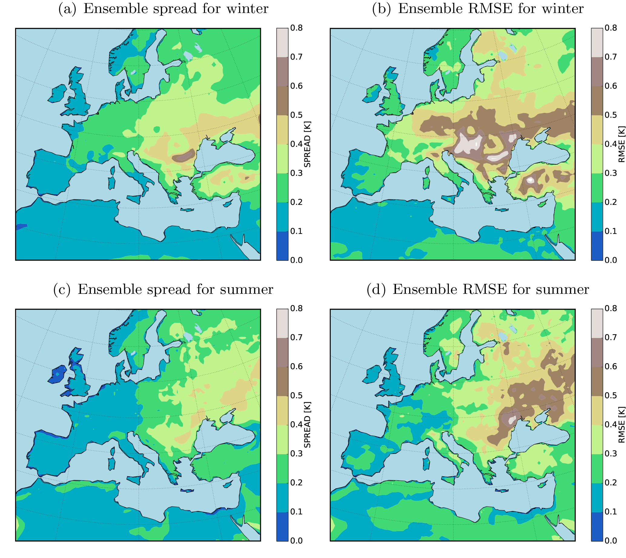
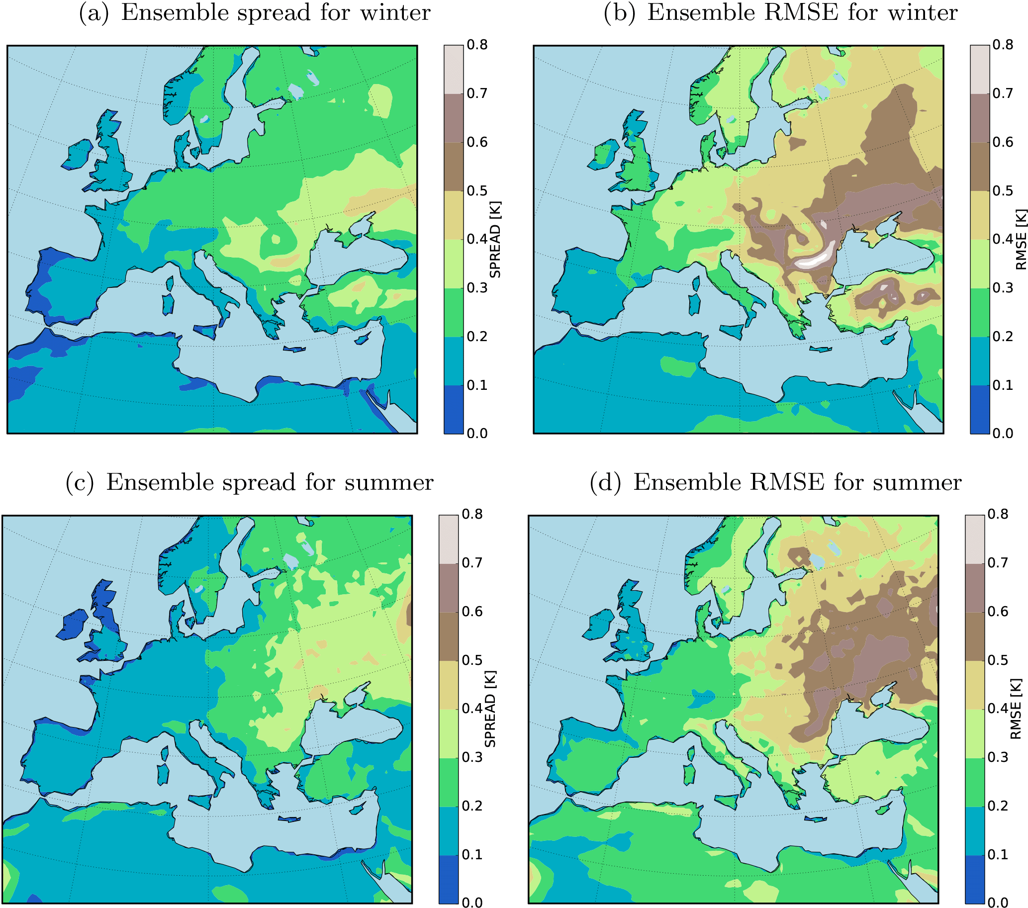
Figure 2 shows the seasonal mean RMSE and the spread of the ensemble for T2M over the evaluation domain. A slight change in the boundary conditions (shifting of the domain) of the model leads to large RMSEs (up to 1 K in seasonal means over 10 years) in the forecasted quantities (Fig. 2). Maximum RMSE values are located on the regions where the spread of the ensemble is also large. An interesting feature of the RMSE pattern is the accumulation of the errors in the center and northeast of the domain for both the winter and summer seasons. West and north of the domain is largely dominated by the ocean where the temperature quantities are forced by the reanalysis data. There is a small difference between the ensemble members on these areas, and the maximum error values are mostly located on land. On the other hand, the maximum lateral inflow occurs on the west and the northwest boundaries. These features have to be considered cautiously when conducting long-term climate simulations using CCLM. The long seasonal time-averaging filter relatively dampens the RMSE and the spread of the ensemble. The errors will increase drastically for daily quantities. One of our main motivations in this paper is to test the usage of OI in the calculation of analysis quantities by assimilating the pseudo-observations and real observations in the free ensemble simulations.

3.2 Constrained ensemble runs

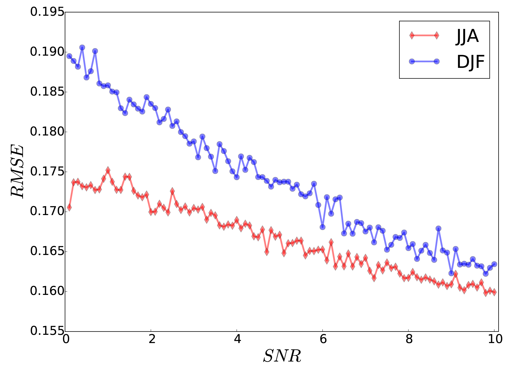
Prior to conducting the analysis calculation, we searched for an optimal correlation length (L) for the covariance localization, which minimizes the RMSE of the analysis. The mean RMSE over the evaluation domain is calculated for different values of L ($\mathrm{0.1}{}^{\circ }\le L\le \mathrm{6}{}^{\circ }$). The RMSE values show a minimum at a correlation length of 1.7^∘ (∼190 km) for summer (JJA) and 2.1^∘ (∼230 km) for winter (DJF) (Fig. 3). For a long-term time averaging, e.g., yearly or decadal periods, the correlation length will increase accordingly (Chen et al., 2015). The increase rate of the RMSE with respect to the correlation length is larger during the summer than in winter. The error reduction of the DA is influenced by the shape of the white noise added to create the pseudo-observation data. Here, we assess the noise levels by the signal-to-noise ratio (SNR), which is the ratio of the variance of clean observation to the variance of added white noise. Figure 4 shows the averaged seasonal near-surface temperature RMSE for the analysis of the ensemble run. The RMSE values are reduced linearly with increasing SNR. In the study of Acevedo et al. (2017), the RMSE values did not change significantly between 2 and 11 SNR values. One possible reason for such a behavior might be due to the regional domain of RCM over Europe, which is dominated by local effects. On the other hand, ∼70 % of the GCM domain in Acevedo et al. (2017) was covered by the oceans where no proxy was assimilated. In our experiment, the field mean filter does not flatten the RMSE reduction rate for larger SNR values over Europe. For the rest of the paper the results are shown with SNR =3.

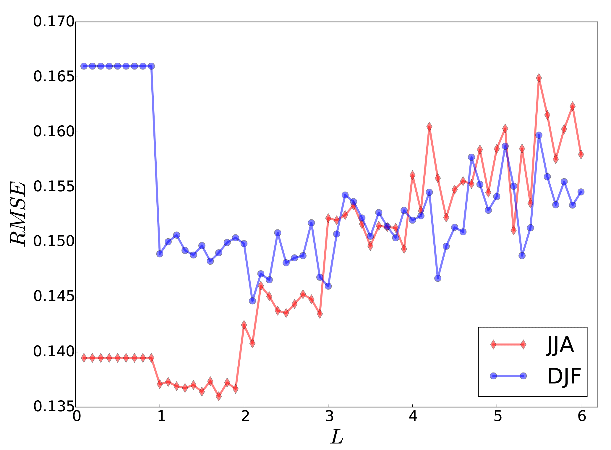
Figure 3 Field mean of RMSE for near-surface temperature (K) analysis over the evaluation domain for different correlation lengths (L, in ^∘C) for winter (blue) and summer (red).

Figure 4 Field mean of seasonal near-surface temperature RMSE (K) of the analysis vs. SNR.

Figures 5 and 6 show the error reduction of the analysis for summer and winter. The assimilation of 500 pseudo-observations has significantly reduced the mean of the errors for both seasons. However, the spread of the errors is more highly reduced in summer than in winter. The regions with the largest error reduction are located in highly populated areas by pseudo-observations (e.g., Germany, Sweden, and Denmark). One interesting feature is the error reduction over the south of the domain where only three observations are available. Usually, in an off-line DA the observational information would not be accumulated over time and could not be conveyed to unobserved regions (Acevedo, 2015). There are two outliers in the ensemble spread during the winter that contribute to the larger error spread during the winter (Fig. 6b). The DA has successfully detected these two outliers and reduced the errors significantly (Fig. 6b).

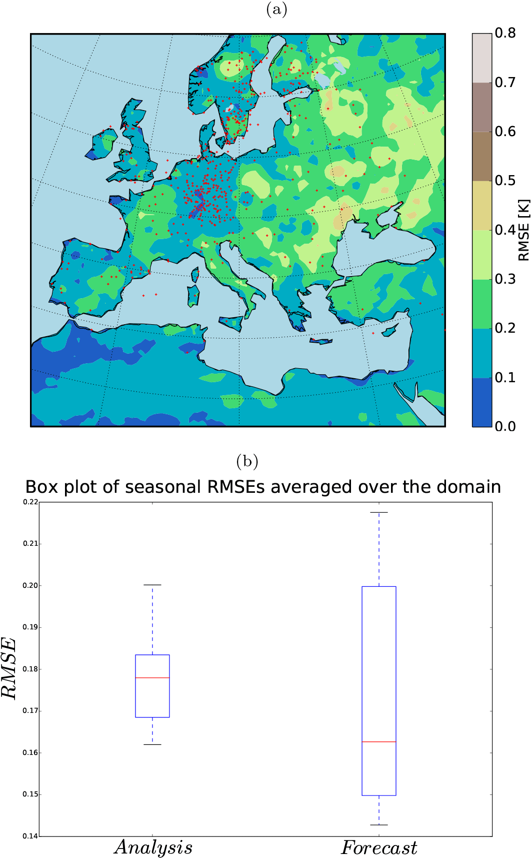
Figure 5 (a) 10-year RMSE (K) of the analysis for summer (JJA) and (b) the field mean RMSE (K) of the analysis and the free ensemble run for summer (JJA).

Figure 6 (a) 10-year RMSE (K) of the analysis for winter (DJF) with and (b) the field mean RMSE (K) of the analysis and the free ensemble run for winter (DJF).

Figure 7 36-year ensemble spread and RMSE for the seasonal mean of 2 m temperature (K).

3.3 Long ensemble runs

As defined by the World Meteorological Organization (WMO) the climate is explained by averaging the weather state for a period of at least 30 years. Therefore, we conducted a new set of five 36-year-long simulations (one nature and four shifted runs). The computational cost of RCM was the only limiting factor to choose this number of members ($\mathrm{5}\times \mathrm{36}=\mathrm{180}$ years of model run). The members were perturbed by shifting the domain four grid points to the northeast, northwest, southwest, and southeast. The 36-year ensemble spread and RMSE show similar patterns as in the previous experiment using 20 members (Fig. 7). The analysis quantities indicate a significant error reduction in both the median and spread of the ensemble (Figs. 8 and 9). Figure 10 illustrates the time evolution of field mean RMSEs for the free ensemble and analysis quantities. There is a linear trend in free-run RMSE. However, the linear trend is removed in the RMSE of the analysis for the summer. This feature was previously observed in an off-line DA experiment using an intermediate complexity model and the EnKF approach (Acevedo et al., 2017). Furthermore, the results show that the analysis RMSEs are significantly reduced compared to the free ensemble run.

Figure 8 (a) 36-year RMSE (K) of the analysis for summer (JJA) and (b) the field mean RMSE (K) of the analysis and the free ensemble for summer (JJA). Red squares indicate the mean of RMSEs.

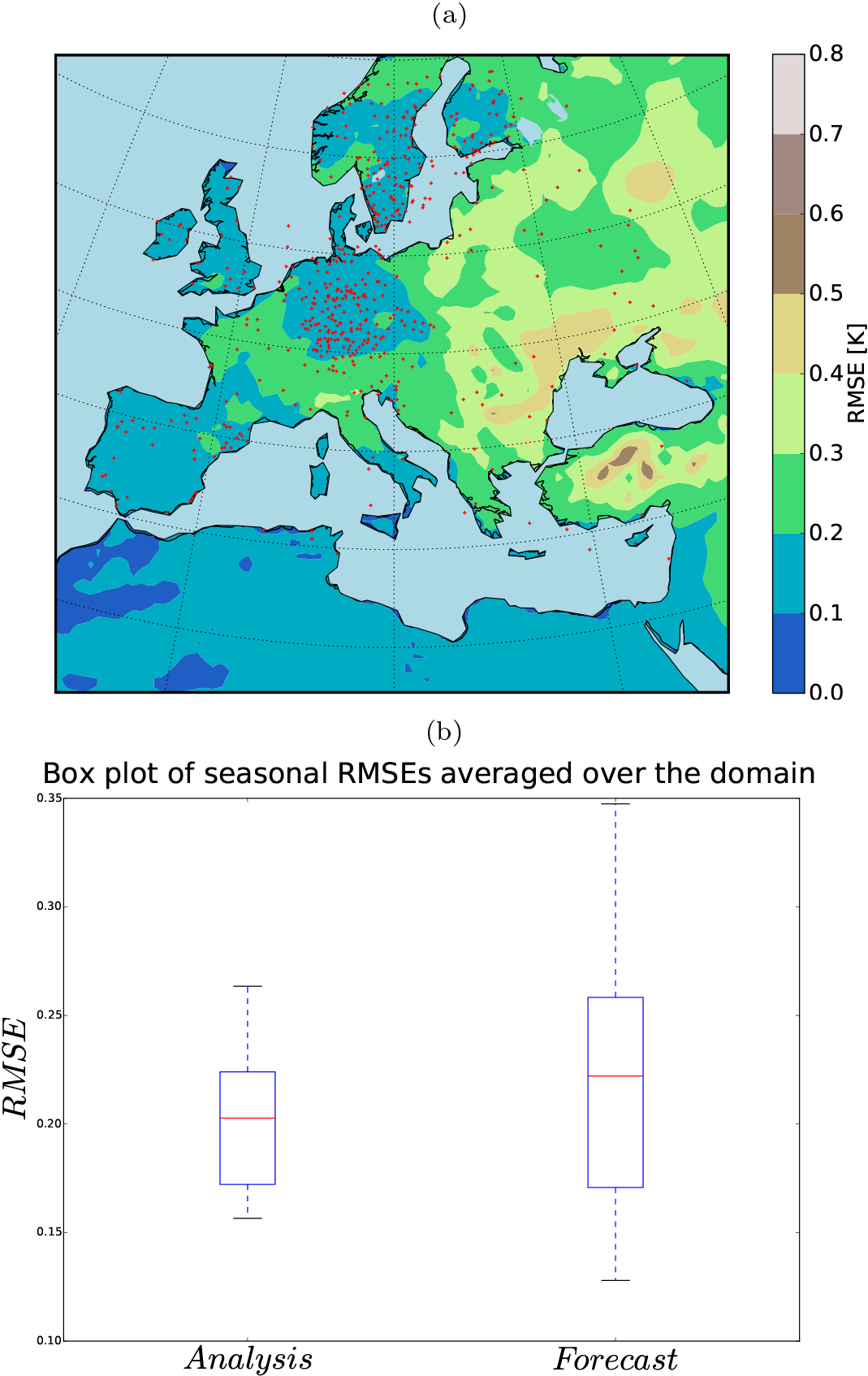
Figure 9 (a) 36-year RMSE (K) of the analysis for winter (DJF) and (b) the field mean RMSE (K) of the analysis and the free ensemble run for winter (DJF). Red squares indicate the mean of RMSEs.

3.4 Random background selection

Following the methodology of Steiger et al. (2014) and Dee et al. (2016) for background selection, using a random climatology from a large climate simulation pool instead of an ensemble simulation at the observation instant might remove the trend previously observed in the RMSEs for winter. Under this setup, the RMSE reduction shows a coherent pattern (Fig. 11a) and the uprising trend in RMSE is removed (Fig. 11b). However, the analysis RMSE mean is in the range of the background state. In our experiment, the background itself had acceptable skills over large portions of the domain. Using random states affects the model skills, for example over the western part of the domain (i.e., Spain, Portugal, France, and Morocco). We conclude that using random states would be beneficial if the model had no significant skills at any region of its domain. Such significant skills of the background might be a characteristic of this particular RCM, which is tuned for Europe.

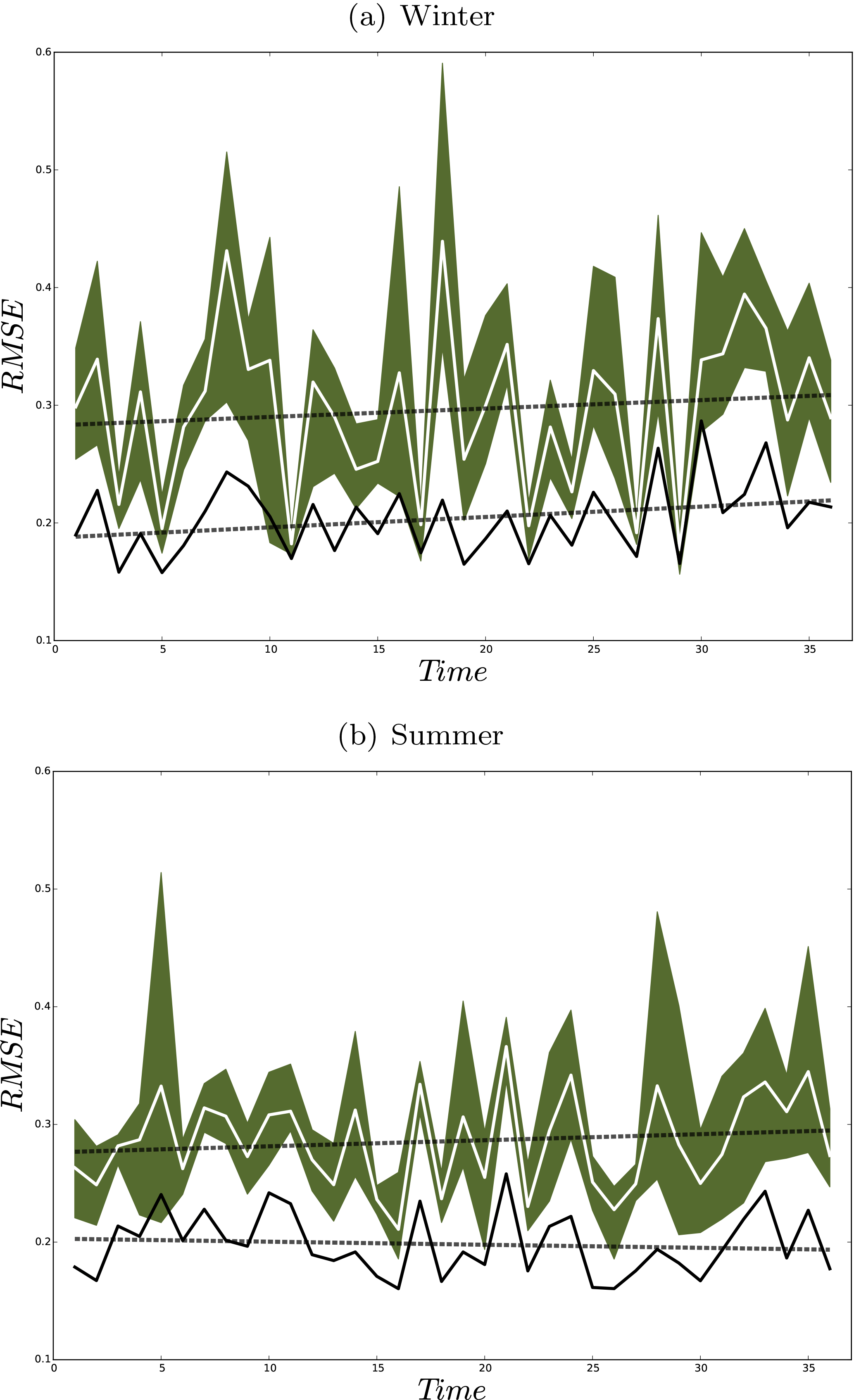
Figure 10 Yearly field mean RMSE (K) of the ensemble mean (white line) and analysis (black line) for winter (a) and for summer (b). Shadings show the ensemble members and dashed lines indicate the linear trends.

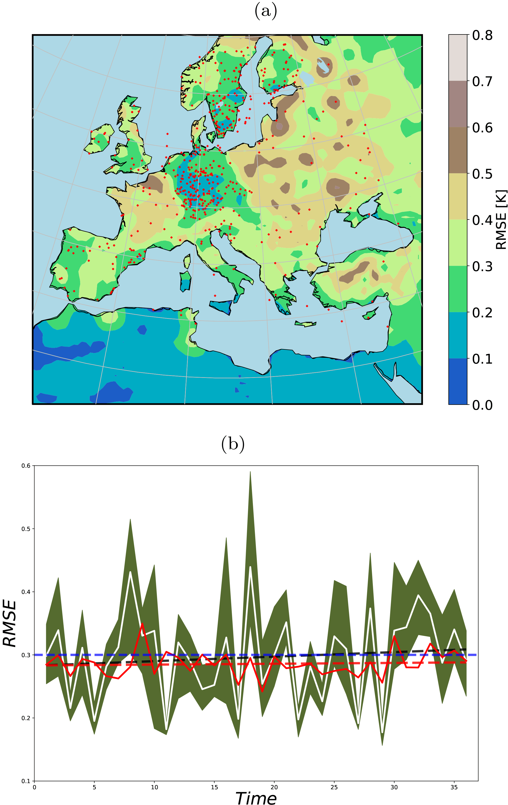
Figure 11 (a) 36-year-averaged RMSE of the analysis using 40 random states as background; (b) field mean of RMSE from the free ensemble (shading shows the ensemble spread, the white line the mean) and from the analysis using random background states (red line). Dashed lines are the linear fits and the blue line shows the 0.3 K RMSE value (plotted only for comparison of the trends).

3.5 Application to a paleo-study: the case of summer temperatures over Europe at the mid-Holocene

A test with the real data will shed light on the applied DA efficiency. Therefore, we design additional experiments using real proxies and precomputed COSMO-CLM simulations at the mid-Holocene. Here, we briefly explain the method and present the results for a single summertime (JJA) time slice of 6000 years before present (6KBP). We use the pollen-based temperature reconstructions of Mauri et al. (2015) as the observation and the model simulations of Russo and Cubasch (2016) as the background in our DA method; 20 % of the proxy data are kept as the test data (randomly selected), and the remaining 80 % as the training dataset. The proxy data do not have a regular timing. Two approaches are applied for averaging the proxy data.

• a.

  Averaging with respect to their distance to the target year (6KBP): a time window centered on the target year (e.g., reference time ±500 years) is chosen and the values as well as their standard errors are weighted by their time distance to the target year. The weights are chosen from a normal distribution with a standard deviation of 100. A total of three weighting time spans are defined (five bins). Figure 12 shows the weights assigned to each time interval with respect to the reference time. The data falling in each particular time bin are weighted equally.

• b.

  Averaging with respect to their uncertainties provided as standard error by Mauri et al. (2015) at the recorded time: all reconstructions within the time window of the reference year ±500 years are chosen. The weighted arithmetic mean of the temperatures and its standard errors are used to calculate the time slice values (6KBP). Each proxy is weighted first by its standard error.

Then the weighted mean is calculated by

$$\begin{array}{}\text{(20)}& \stackrel{\mathrm{‾}}{x}={\displaystyle \frac{{\sum }_{i=\mathrm{1}}^n\left(x_i{\mathit{\sigma }}_i^{-\mathrm{2}}\right)}{{\sum }_{i=\mathrm{1}}^n{\mathit{\sigma }}_i^{-\mathrm{2}}}}.\end{array}$$

The uncertainty of the weighted mean is given then by

$$\begin{array}{}\text{(21)}& {\mathit{\sigma }}_{\stackrel{\mathrm{‾}}{x}}^{\mathrm{2}}={\displaystyle \frac{\mathrm{1}}{{\sum }_{i=\mathrm{1}}^n{\mathit{\sigma }}_i^{-\mathrm{2}}}},\end{array}$$

where σ is the standard error. Figure 13 shows the schematic of weighting the observations with respect to their standard errors.

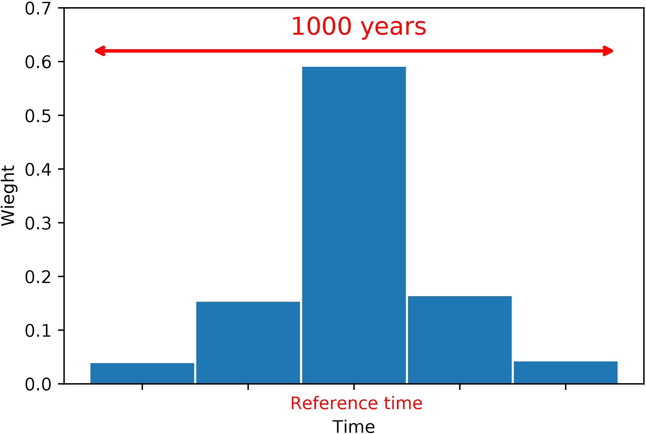
Figure 12 Schematic showing the weights for observations with respect to their distance to the target year. A time window of 1000 years is chosen. The observations are weighted depending on their distances to the reference time.

Finally, for the model, the 25-year time average is assigned as the expected value and the standard deviation from the mean as the uncertainty measure. Figure 14 shows the schematic of the approach. Please note that, here, a single model run of 25 years is used as the background. We assume that each year of the model simulation could serve as an ensemble member for the target time slice (6KBP). Therefore, the analysis is done for a single step using the background information of the 25 years. Figure 15a shows the analysis results for summer T2M temperature anomalies from the preindustrial time (6KBP–0.2KBP) over Europe obtained by the application of approach (a) for averaging the proxy data. The testing proxy data are represented by circles, while their standard error is represented as superimposed squares. The analysis and the proxy show a good agreement, especially for proxy records with low standard error. In contrast, the model forecast (without assimilation) and the proxies (Fig. 15b) show little agreement. The assimilated reconstructions are shown in Fig. 16. The positive anomalous region over Romania in the analysis is due to the cluster of proxy data with low standard error over this region. By applying method (b) for averaging, the analysis pattern is very similar to the previous method (Figs. 17 and 18). Overall, we conclude that the proposed DA approach contributes to the error reduction in the analysis values for which the pure model outputs might not capture the local patterns.

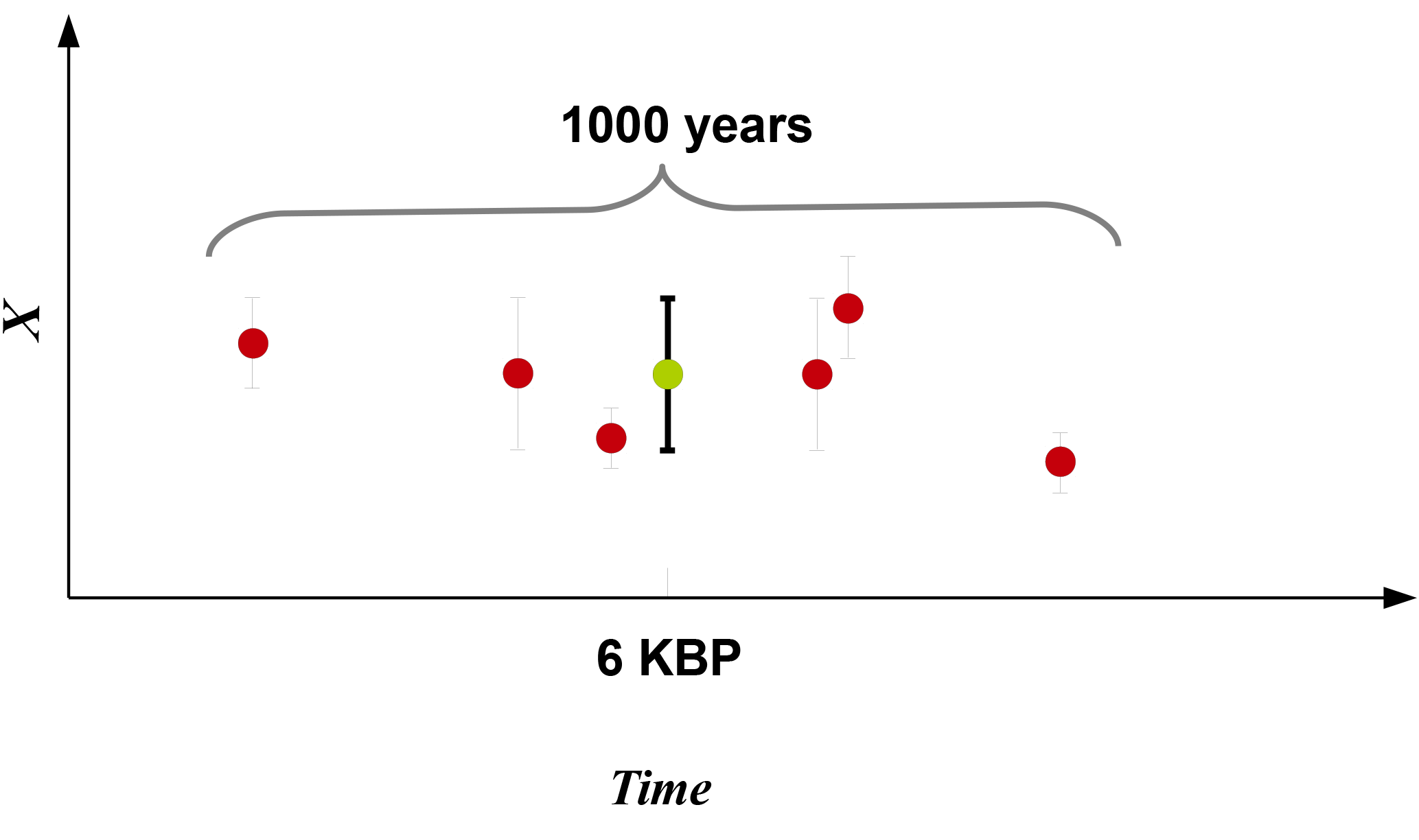
Figure 13 Schematic showing the weights for observations with respect to their standard error. A time window of 1000 years is chosen. The red dots represent the proxies in the 1000-year time window and the green dot represents the weighted mean.

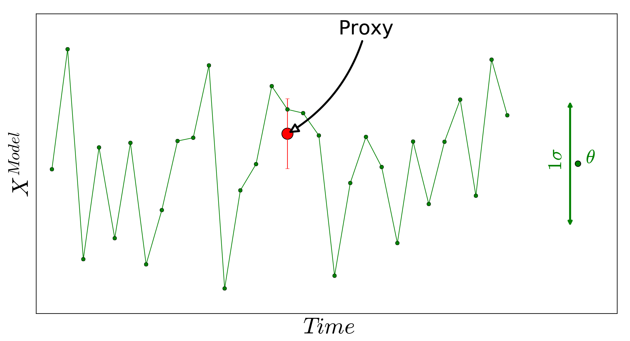
Figure 14 Schematic showing how the expected value (the mean) and the deviation from the mean for the time slice simulation are selected. The model simulation is 25 years long. The green line represents the model state.

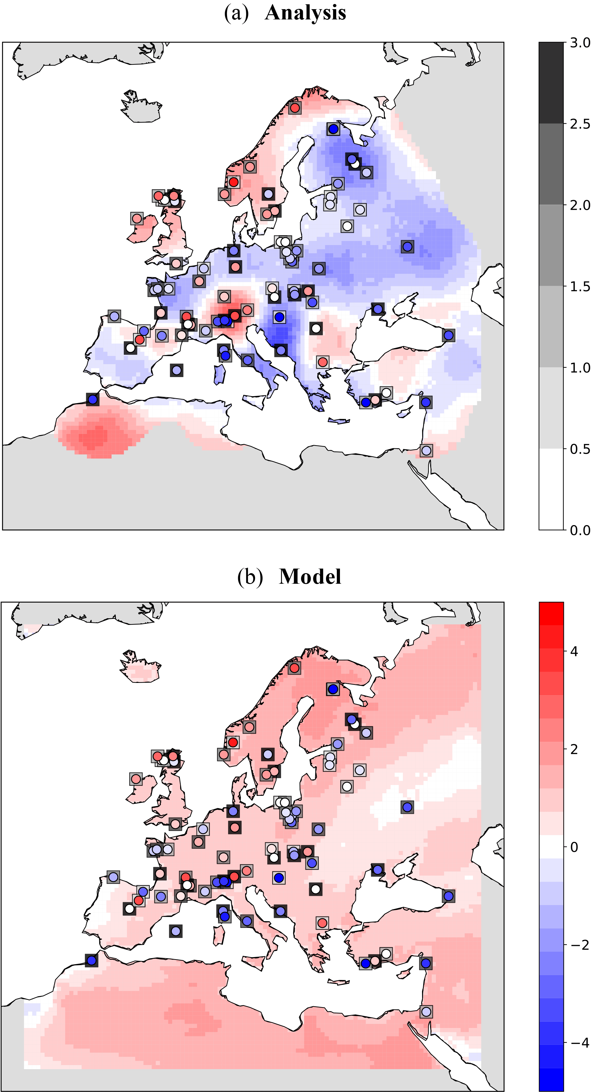
Figure 15 DA results of T2M during summer at 6KBP using weighted arithmetic mean by time distances: (a) analysis values along with the testing observations (circles) and their standard error (squares). Values with an error covariance of analysis greater than 0.9 are masked out from analysis and (b) the model forecast.

We have to mention that the analysis presented here is based on the combination of the proxy reconstructions and the climate model, and any interpretation of the patterns should take into account the uncertainties provided by these two sources of information. Several factors have driven our decision to apply the proposed DA method to this particular paleoclimate case study. Among these, the most important one was the attempt to contribute to the reconstruction of summer temperatures over the Mediterranean region at the mid-Holocene. This has been the subject of a long-standing debate within the paleoclimate community: on the one hand, climate model simulations (Braconnot et al., 2007; Fischer and Jungclaus, 2011; Bonfils et al., 2004; Russo and Cubasch, 2016) and some reconstructions based on specific proxy types (such as chironomids, Samartin et al., 2017) have shown that the area was characterized by warmer summer conditions with respect to present day; on the other hand, climate reconstructions based on other proxies, in particular the ones based on pollen data (Cheddadi et al., 1996; Davis et al., 2003; Mauri et al., 2015), have given support to the idea of opposite, colder conditions over the area.

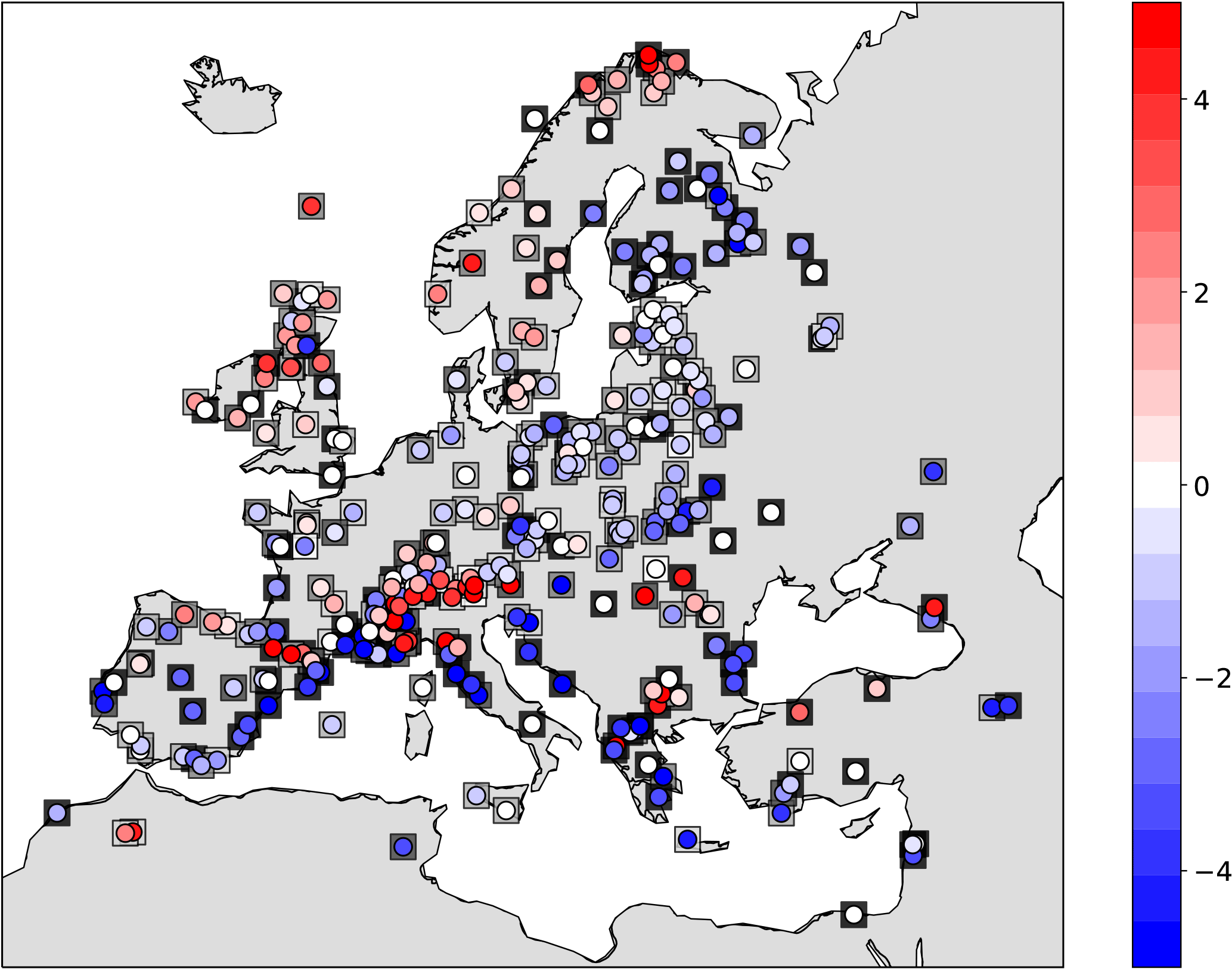
Figure 16 Weighted arithmetic mean using time distances: anomalies (6KBP–0.2KBP) of assimilated observations (circles) superposed on their standard errors (squares) with values in K. Color bar of the standard errors as in Fig. 15a.

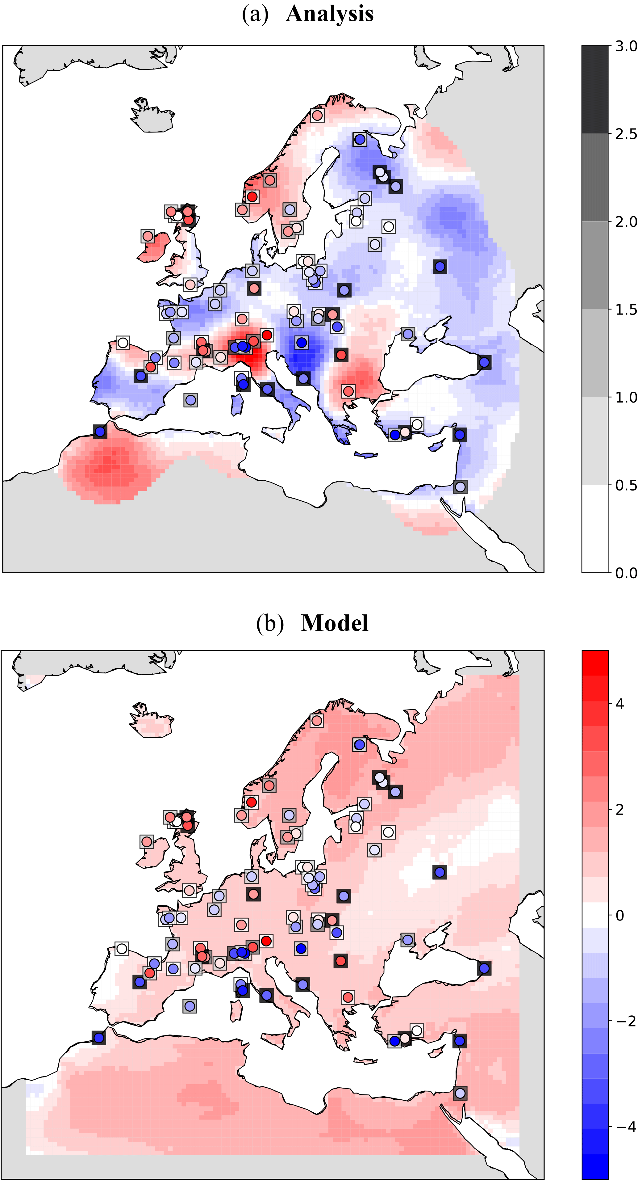
Figure 17 DA results of T2M during summer at 6KBP using weighted arithmetic mean by standard errors: (a) analysis values along with the testing observations (circles) and their standard error (squares). Values with an error covariance of analysis greater than 0.9 are masked out from analysis and (b) the model forecast.

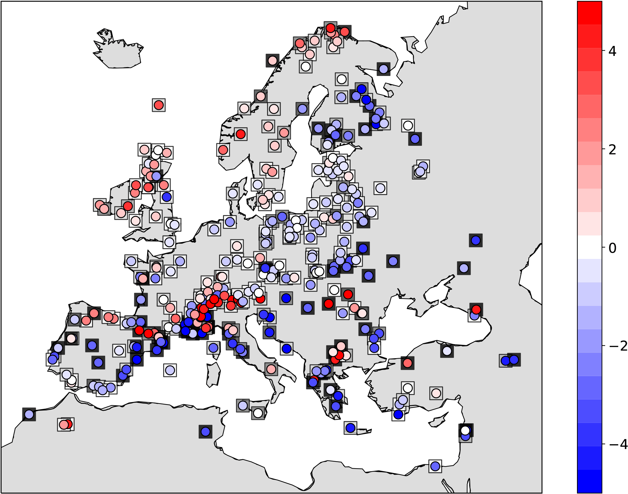
Figure 18 Weighted arithmetic mean using standard errors: anomalies (6KBP–0.2KBP) of assimilated observations (circles) superposed on their standard errors (squares) with values in K. Color bar of the standard errors as in Fig. 17a.

This dualism seemed to be finally solved in a recent study by Samartin et al. (2017), in which they showed that summer temperatures reconstructed from chironomids over northern Italy were higher at the mid-Holocene compared to present times. This pattern was also captured by other proxy records from different parts of the Mediterranean area and the results of climate models. Indeed, they criticized temperature reconstructions based on pollen data for this region due to the fact that Mediterranean vegetation is mainly controlled by effective precipitation rather than temperatures. Our results are in agreement with Samartin et al. (2017) over northern Italy and the Alpine region despite the presence of heterogeneous colder conditions over southern Europe. Indeed, we believe that this complicated puzzle is not solved yet and more efforts should be put into joint cooperation among different proxy experts and climate modelers. We emphasize the fact that data assimilation could be considered a very useful tool for the syntheses of different climate records and physical representation of the climate system. This could offer a more reliable picture than individual proxy datasets or a single climate simulation.

4 Conclusion and discussion

Using a computationally fast DA approach, we assimilated pseudo-observations and real observations within an ensemble of precomputed RCM simulations. The ensemble is created by slightly perturbing the boundary and initial conditions of its members via the domain-shifting method. In the framework of a perfect model experiment the performance of free ensemble and analysis quantities is evaluated. Such experiments facilitate the estimation of observation, background, and analysis error. In the first set of experiments, we conducted an ensemble of 20 simulations driven by ERA-Interim for the duration of 10 years. The nearest-neighbor interpolation is applied as the observation operator plus a random white noise with known standard deviation to create a set of pseudo-observations from the nature run. Pseudo-observations are assimilated within the ensemble of RCM runs by means of the OI approach. By conducting a set of simulations using four perturbed members and a nature run, we repeated the perfect model experiment for a time expansion of 36 years. This allowed us to draw conclusions on the time evolution of the DA skill for a typical climatological period (more than 30 years). In a final step, we assimilated pollen-based temperature reconstructions of the mid-Holocene precomputed RCM simulation with a 25-year duration at 0.44^∘ horizontal resolution and compared the results with a test dataset.

The comparison of ensemble mean of COSMO-CLM model outputs and the pseudo-observations shows that the model seems to be well tuned for central Europe. A region of significant model bias for both the winter and summer seasons is located over the east side of the domain. This area is located far from the ocean where the ERA-Interim data are prescribed (no coupled ocean was implemented). Therefore, we speculate that the model generates more variabilities and is free to evolve over this region (answer to question (i) in the Introduction). Furthermore, we iterated the DA experiment on different values of correlation length for the summer and winter to find the optimal correlation length quantity. The optimum radius of correlation is found to be 1.7^∘ (∼190 km) for summer (JJA) and 2.1^∘ (∼230 km) for winter (answer to question (ii) in the Introduction). Afterward, we showed that the skill of OI is linearly influenced by the SNRs used to create the noisy observations (answer to question (iv) in the Introduction).

Our experiments showed that the ensemble OI is useful for conducting an analysis of seasonally averaged quantities (answer to question (iii) in the Introduction). Despite the inhomogeneity of the observation distribution over the domain, the analysis presents error reduction over most of the domain. For a small ensemble with a longer integration period of 36 years, the analysis significantly outperforms the ensemble mean. However, for the winter season, the analysis error increases with time and it consists of the same rising trend as in the error of the ensemble mean. For the summertime the trend was removed in the analysis. This was previously observed in the study of Acevedo et al. (2017) by assimilating summertime tree ring width pseudo-observations in an AGCM using the EnKF. However, our simulations are very short compared to the one of Acevedo et al. (2017). Using a random climatology from a large climate simulation pool as the background instead of using an ensemble simulation at the observation period, following Steiger et al. (2014) and Dee et al. (2016), has removed the winter RMSE trend. However, the mean RMSE value was not significantly reduced compared to the background. For the real-world experiment, the magnitude of the analysis skills might have been influenced by using the climate of a single run for the background state. As long RCM runs are now available (i.e., this study; Russo and Cubasch, 2016; Fallah et al., 2016; the Coordinated Downscaling Experiment – European Domain, EURO-CORDEX), which can serve as a large climate analog for the background state, we suggest further DA experiments to reconstruct high-resolution climate fields given the time-averaged observations.

In this paper inverse model outputs (temperature reconstructions) are exerted directly. In a real-world experiment, it is recommended to use proxy system models (PSMs) to remove the simplistic assumptions of inverse climate modeling and let the assimilation take place at the observation space instead of the model space (Dee et al., 2016; Dolman and Laepple, 2018). However, there is a huge gap in the recent knowledge of PSMs and more efforts should be made to move the knowledge of forward proxy modeling one step forward (Acevedo et al., 2017). For example, a previous study (Acevedo et al., 2017) using a proxy forward model showed that the error reduction for other model values like precipitation was not significant. In such setups, the success of paleo-DA is largely affected by the skill of the proxy forward model.

A major drawback of our experiment is the linearity assumption of the forecast model and the Gaussianity of the observation and model errors. In OI the background error covariance is usually prescribed and calculated once during the entire assimilation procedure. Our experiment showed that although the spread of the ensemble increases slightly in time, each individual member and the ensemble mean show a similar trend. This similar behavior of the members might be due to the systematic behavior of the CCLM. We suggest a multi-model ensemble approach to account for a wider range of internal variabilities. However, conducting such experiments is prohibitively expensive with today's computational powers.