the Creative Commons Attribution 4.0 License.
the Creative Commons Attribution 4.0 License.
 | 15 Aug 2018
Solar and volcanic forcing of North Atlantic climate inferred from a process-based reconstruction
Christophe Sturm
Florian Adolphi
Bo M. Vinther
Martin Werner
Gerrit Lohmann
Raimund Muscheler
The effect of external forcings on atmospheric circulation is debated. Due to the short observational period, the analysis of the role of external forcings is hampered, making it difficult to assess the sensitivity of atmospheric circulation to external forcings, as well as persistence of the effects. In observations, the average response to tropical volcanic eruptions is a positive North Atlantic Oscillation (NAO) during the following winter. However, past major tropical eruptions exceeding the magnitude of eruptions during the instrumental era could have had more lasting effects. Decadal NAO variability has been suggested to follow the 11-year solar cycle, and linkages have been made between grand solar minima and negative NAO. However, the solar link to NAO found by modeling studies is not unequivocally supported by reconstructions, and is not consistently present in observations for the 20th century. Here we present a reconstruction of atmospheric winter circulation for the North Atlantic region covering the period 1241–1970 CE. Based on seasonally resolved Greenland ice core records and a 1200-year-long simulation with an isotope-enabled climate model, we reconstruct sea level pressure and temperature by matching the spatiotemporal variability in the modeled isotopic composition to that of the ice cores. This method allows us to capture the primary (NAO) and secondary mode (Eastern Atlantic Pattern) of atmospheric circulation in the North Atlantic region, while, contrary to previous reconstructions, preserving the amplitude of observed year-to-year atmospheric variability. Our results show five winters of positive NAO on average following major tropical volcanic eruptions, which is more persistent than previously suggested. In response to decadal minima of solar activity we find a high-pressure anomaly over northern Europe, while a reinforced opposite response in pressure emerges with a 5-year time lag. On centennial timescales we observe a similar response of circulation as for the 5-year time-lagged response, with a high-pressure anomaly across North America and south of Greenland. This response to solar forcing is correlated to the second mode of atmospheric circulation, the Eastern Atlantic Pattern. The response could be due to an increase in blocking frequency, possibly linked to a weakening of the subpolar gyre. The long-term anomalies of temperature during solar minima shows cooling across Greenland, Iceland and western Europe, resembling the cooling pattern during the Little Ice Age (1450–1850 CE). While our results show significant correlation between solar forcing and the secondary circulation pattern on decadal (r=0.29, p<0.01) and centennial timescales (r=0.6, p<0.01), we find no consistent relationship between solar forcing and NAO. We conclude that solar and volcanic forcing impacts different modes of our reconstructed atmospheric circulation, which can aid in separating the regional effects of forcings and understanding the underlying mechanisms.
Please read the corrigendum first before continuing.
-
Notice on corrigendum
The requested paper has a corresponding corrigendum published. Please read the corrigendum first before downloading the article.
-
Article
(8868 KB)
- Corrigendum
-
Supplement
(955 KB)
-
The requested paper has a corresponding corrigendum published. Please read the corrigendum first before downloading the article.
- Article
(8868 KB) - Full-text XML
- Corrigendum
-
Supplement
(955 KB) - BibTeX
- EndNote


Climate variability in the North Atlantic region can, to a large extent, be explained by different modes of atmospheric circulation. This is particularly true for the variability during winter. The dominant mode is the North Atlantic Oscillation (NAO), which is a measure of the strength and position of the westerly winds across the North Atlantic. Traditionally, the NAO is defined as the pressure difference between Iceland and the Azores (Walker and Bliss, 1932). Using gridded data, the NAO can be defined as the first principal component (PC1) of sea level pressure (SLP) in the North Atlantic region (Hurrell et al., 2003). The second most important pattern, PC2 of SLP, is often referred to as the Eastern Atlantic Pattern (Wallace and Gutzler, 1981). Modes of circulation can also be identified using cluster analysis, and the secondary modes include Atlantic ridge- and trough-type variability, characterized by mid-Atlantic and Scandinavian blockings, respectively (Hurrell et al., 2003). These different modes, for example, determine the severity of European winters (Hurrell et al., 2003). In paleoclimate studies, climate variability and changes in atmospheric circulation are often attributed to external forcing related to solar variability or volcanic eruptions (e.g., Ortega et al., 2015; Wang et al., 2017). Using reanalysis of weather observations (1871–2008) it has been shown that a positive phase of the NAO occurs in the winters following major tropical volcanic eruptions, while climate models generally fail to reproduce this dynamical response to the forcing (Driscoll et al., 2012; Zambri and Robock, 2016; Swingedouw et al., 2017). For the past millennium, Ortega et al. (2015) found a positive NAO response in the second winter following the 11 largest tropical eruptions in their reconstructed NAO. However, more persistent climate effects of volcanic eruptions were found by Sigl et al. (2015) who inferred cooler European summer temperatures lasting up to 10 years following major tropical eruptions during the past 2500 years, raising the question if a more persistent impact on winter circulation also can be expected. The observed NAO does not show a consistent correlation to the solar forcing (Gray et al., 2013). However, anomalies in SLP during 1950–2010 exhibit a NAO-like pattern correlated to the 11-year solar cycle (Ineson et al., 2011; Adolphi et al., 2014). It has been hypothesized that solar-induced anomalies in the stratosphere can propagate to the troposphere (Haigh and Blackburn, 2006; Kodera and Kuroda, 2005) possibly synchronizing NAO variability to the 11-year solar cycle (Thieblemont et al., 2015) with a maximum response lagging 2–4 years due to ocean memory effects (Scaife et al., 2013; Gray et al., 2013). Several paleoclimate studies have indicated solar influences on climate in the North Atlantic region on centennial timescales (Bond et al., 2001; Sejrup et al., 2010; Moffa-Sanchez et al., 2014; Adolphi et al., 2014; Jiang et al., 2015), and it has been suggested that the climate conditions during the Little Ice Age was linked to negative NAO forced by low solar activity (Shindell et al., 2001; Swingedouw et al., 2011). However, the nature of the solar influence in terms of mechanisms and dynamical response is debated.
Our understanding of past climate dynamics and the impact of external forcings relies heavily on analysis of past changes. Gridded data sets of climate variables based on meteorological observations have been developed for these purposes (Compo et al., 2011). Such reanalysis data sets are constrained in quality and coverage back in time due to sparse instrumental data, and we rely on climate reconstructions based on proxy data to go beyond the instrumental era. Previously, reconstructions of climate indices (such as, for example, the NAO) have been site-based, with the reconstruction essentially done by extrapolating observed empirical relationships back in time. This approach results in a wide spread of reconstructions of past atmospheric circulation modes (Pinto and Raible, 2012). Recently, efforts have been done to develop reanalysis-type climate reconstructions based on climate proxy data. However, those reconstructions are focused on annual mean data, not taking into account the migration of circulation patterns from summer to winter (Hurrell et al., 2003), and have low skill for atmospheric circulation over the North Atlantic (Hakim et al., 2016; Steiger et al., 2017).
Stable water isotope ratios in ice cores carry quantitative information about past climate (Johnsen and Vinther, 2007). For Greenland ice cores, seasonal isotope variability is attainable. In particular, the winter isotope signal has been shown to be highly correlated to atmospheric circulation and temperature (Vinther et al., 2003, 2010). However, the strength of the relation between the main patterns of variability of the ice core isotope signal and the NAO has been suggested to vary in strength (Vinther et al., 2003), indicating that a simple (regression-based) relation between the ice core records and NAO bears large uncertainties for reconstruction purposes.
Here we present a climate reconstruction for the North Atlantic region for winter covering 1241–1970 CE, and analyze the impact of solar and volcanic forcing. For our reconstruction we combine a simulation using a coupled atmosphere–ocean model with stable isotope diagnostics embedded in the hydrological cycle with eight seasonally resolved isotope records from Greenland ice cores. We do not calibrate the reconstructed meteorological variables to observations, as we solely rely on matching the modeled isotopic composition to the ice core data. Testing the reconstruction against reanalysis data and observations, the reconstruction has good skill not only for the NAO but also for secondary circulation modes. We find the average response to major tropical volcanic eruptions to be a positive NAO for the five consecutive winters after eruptions, which is more persistent than previous studies have shown. However, we find no persistent relationship between solar forcing and the NAO. On the other hand, we find a strong impact of solar forcing on the secondary modes of circulation represented by PC2 of reconstructed SLP. We achieve the strongest correspondence between the solar forcing and reconstructed PC2 of SLP with a time lag of 5 years, indicating that an atmosphere–ocean feedback is in play. Taking this time lag into account, we find a consistent relationship between PC2 of the reconstructed SLP and solar forcing on decadal to centennial timescales.
2.1 Model simulation
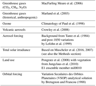
We use the isotope-enabled version of the atmosphere–ocean model ECHAM5/MPI-OM (Werner et al., 2016) to simulate the period 800–2000 CE forced by greenhouse gases, volcanic aerosols, total solar irradiance, land use and orbital forcing (see Table 1). For our study, ECHAM5 is run with a T31 spectral resolution () with 19 vertical layers, 5 of which are in the stratosphere. Our simulation uses a similar setup as the E1 COSMOS ensemble by Jungclaus et al. (2010), except for an updated solar forcing (see Sect. 2.2) and fully prescribed CO2, where the E1 simulations incorporate a carbon cycle module. We apply the identical physical general circulation models (GCMs) (ECHAM5/MPI-OM) as the E1 ensemble, as well as similar forcings, and our simulation generally yields a very similar climate as the E1 ensemble. The performance of the atmospheric component of the model used in this study, ECHAM5-wiso, was evaluated for the Arctic region and Antarctica using different configurations of spatial resolution by Werner et al. (2011). For the configuration used in this study (T31), the model has a warm bias and is not depleted enough in δ18O; however, the climatological relation between δ18O and temperature compares well to observations, despite the relatively course resolution. Greenland is represented by 50 grid points in the simulation.
MacFarling Meure et al. (2006)Marland et al. (2003)Paul et al. (1998)Crowley et al. (2008)Tanre et al. (1984)Lefohn et al. (1999)Muscheler et al. (2016, 2007)Pongratz et al. (2008)Jungclaus et al. (2010)Bretagnon and Francou (1988)Table 1List of forcings for the ECHAM5/MPI-OM model simulation.
2.2 Solar forcing
The solar forcing record employed in this study is based on the solar modulation record inferred from the combined neutron monitor and tree-ring 14C data (Muscheler et al., 2016, 2007). In contrast to Schmidt et al. (2011, 2012) it covers the last 2000 years and consistently uses the solar modulation record for the complete period, while in Schmidt et al. (2011, 2012) the 14C-based record is combined with sunspot-based data for the period after 1850 CE. Therefore, our approach employs an internally self-consistent forcing record for the last 2000 years, and agrees well with the latest recommended solar forcing reconstruction for the past millennium (Jungclaus et al., 2017). The 11-year solar cycle is based on the neutron monitor and 14C data for the last 500 years where the underlying data has a sufficiently high temporal resolution. For the period before 1500 CE an artificial 10.5-year cycle was added and the phasing was adjusted to allow for a smooth connection to the subsequent start of the data-based solar cycle. The amplitude of the solar cycle modulation was inferred from the data-based part of the record, i.e., by employing the relationship between the solar cycle amplitude and the longer-term solar modulation levels (11-year averages) during last 500 years. This solar modulation record was scaled to the total solar irradiance (TSI) record by Schmidt et al. (2011, 2012) including longer-term trends in TSI (see “MEA (back)”, Fig. 8 in Schmidt et al., 2011). This was done by linearly transforming the solar modulation to a TSI record in order to reproduce the long-term changes (11-year average) in TSI from the Maunder minimum to the most recent 50 years, i.e., leading to a similar range of long-term TSI changes as suggested by Schmidt et al. (2011).
2.3 Climate reconstruction
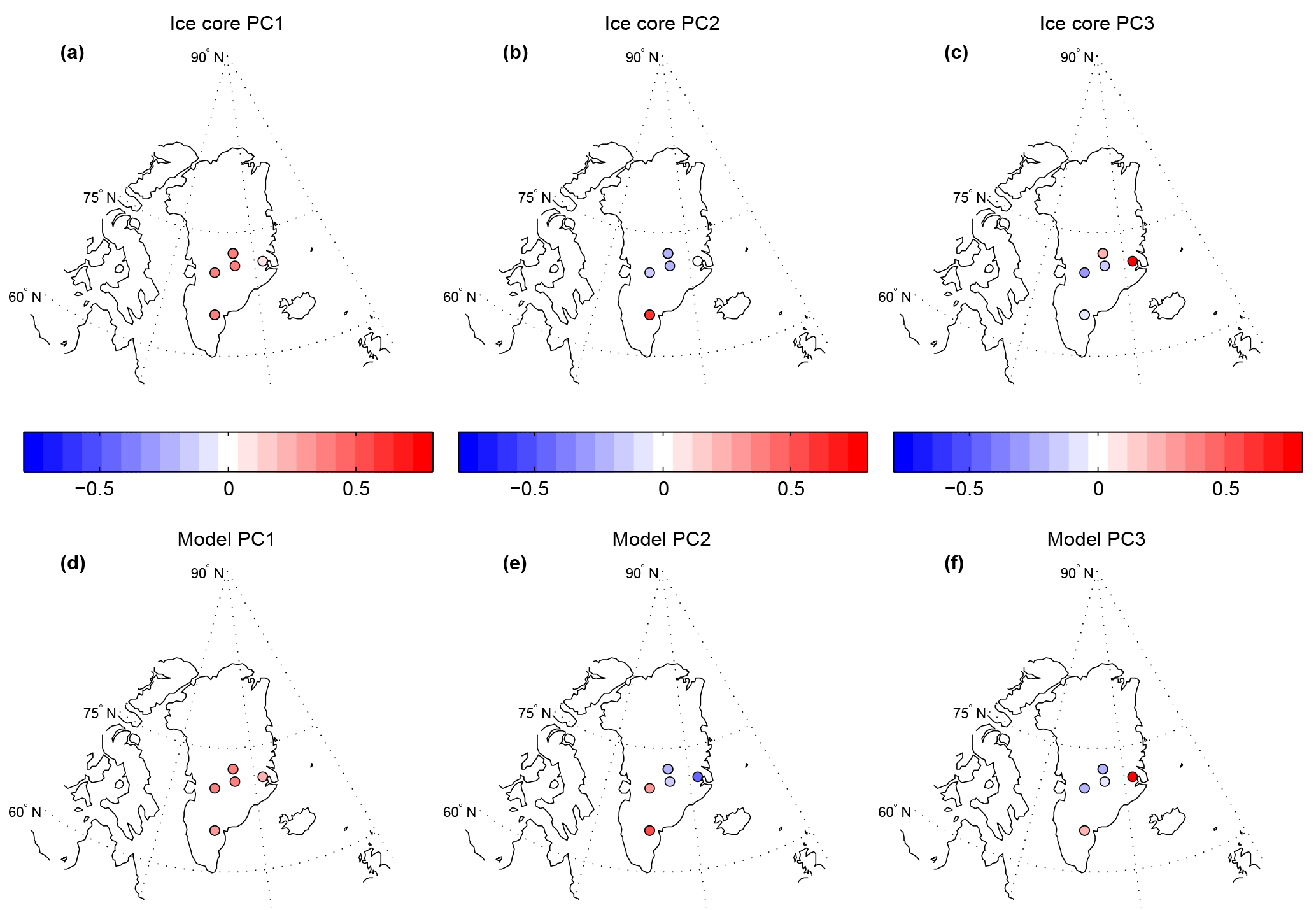
Figure 1Spatial patterns of the three main modes of variability in the δ18O ice core records used in this study and the modeled modes of variability at these sites. The pattern of the loadings on ice core δ18O PCs are shown in (a, b, c) and modeled loadings on δ18O PCs at the ice core sites are shown in (d, e, f).
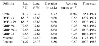
We use winter seasonal means (November–April) for eight Greenland ice cores (Vinther et al., 2010) for the period 1241–1970 CE (Table 2). All ice cores are synchronized via volcanic reference horizons, and the dating uncertainty is estimated to 1 year for the oldest parts of the records used here (Vinther et al., 2006). Under the assumption that δ18O in precipitation is a result of a number of processes mainly determined by atmospheric variability, we treat each year of the model run (see above) as a sample in a sampling space relating δ18O in precipitation with circulation, temperature, etc. By extracting precipitation-weighted winter seasonal means (November–April) of δ18O from the model at the eight ice core sites, we can find the model years best matching the isotope pattern of each winter in the ice core data. In order not to over-fit noise in the ice core data (post-depositional processes etc. White et al., 1997), we first perform a principal component analysis of the ice core δ18O and the model δ18O from grid cells covering the investigated ice core sites. We retain the first three PCs explaining a total of 60 % and 97 % of variability in the ice core and model δ18O, respectively. The loadings of the 3 PCs for the model data match the loading of the ice core data well (Fig. 1). Notice that this step is done without performing any selection of the model data, meaning that the modeled spatiotemporal variability in the δ18O in precipitation corresponds well to that of the ice core data. As we only explain part of the variability in the δ18O data using the first 3 PCs, we use an ensemble approach to take into account that the matching of a given ice core δ18O pattern will result in a suite of well-matching model years. To match each year in the ice core data, the model data are evaluated using a χ2 measure between the 3 PCs of Greenland ice core δ18O and the 3 PCs of the modeled δ18O:
where PC(k)model and PC(k)icecore are the values from a given year of the normalized time series of model and ice core δ18O PCs, respectively. Each model year is evaluated against each year of the ice core data and then sorted in ascending order of the quality of the fit. This creates 1201 (number of model years, see above) fits of model output for each year of the ice core data, i.e., 1201 resampled (with replacement) and sorted model years for the entire length of the ice core data (1241–1970 CE). We define the sorted model output as ensemble members, such that the best fitting model year, for each year of the ice core data, belongs to ensemble member 1, the second best fitting model years belong to ensemble member 2, and so forth. Using a Chi-square goodness-of-fit test, with respect to the measure in Eq. (1), we evaluate the ensemble members against the PCs of Greenland ice core δ18O and reject model fits with likelihood p>0.01 of not fitting the ice core data. This leaves us with 39 time series of reshuffled model data fitted to the ice core data. The temporal succession of the reshuffled model output does not resemble the order of the years in the original model run, and there are no systematic preferences of the method to pick certain time periods of the model run to match certain time periods of the reconstruction. For example if we exclude the years 1851–2000 from the model run and perform the reconstruction using the remaining years, the reconstruction is almost identical to the reconstruction using all model years. This also means that the timing of the forcing used for the model run has no relation to the timing or impact of specific forcings in the reconstruction, i.e., the forcings of the model run effectively serve to produce enough range in order to match the simulation to the isotope variability in the ice cores. Since the timing of the forcings used for the model simulation is not a factor influencing the reconstruction, the model performance for the response to forcings does not influence the reconstruction. We treat the 39 model fits as an ensemble solution fitting the model output to the ice cores δ18O, and we calculate the ensemble mean reconstructed δ18O and the standard deviation showing the ensemble spread. For the target climate variables (SLP, T2m) we extract the DJF ensemble mean corresponding to the reconstructed δ18O constituting the reconstruction of these variables. Note that using this approach the method is optimized to fit modeled δ18O to ice core δ18O records and, in contrast to presently existing reconstructions, it is not calibrated to match observations of any of the target variables of the reconstruction (i.e., SLP or T2m).
Table 2Site details of ice core records used for the reconstruction (Vinther et al., 2010). BC* indicates the at the core was drilled to bedrock.
As a first test we correlate the reconstructed δ18O to winter means of ice core data from 20 cores covering the last 200 years of the reconstruction, i.e., including ice core data not part of the reconstruction. The correlation shows a spread between 0.4 and 0.9 with the highest correlations found for the high accumulation sites, and where multiple ice cores for the same site are used for the reconstruction. This supports the idea that the skill of the model fit to the seasonal ice core data is largely limited by the signal-to-noise ratio of the ice core data (Fig. S1 in the Supplement). High accumulation sites are generally less sensitive to wind scoring and post-depositional diffusion. Despite using the variability of the PCs to fit the model output to the ice core data, the reconstructed range of δ18O matches the ice core data well (Fig. S2). Furthermore we test the fit of the reshuffled model δ18O to the ice core data of the eight sites to investigate if any time periods stand out, as well as the mean fit of the method across the whole period of the reconstruction. We find no trends in the performance in terms of fitting the modeled PCs to the ice core data PCs. As the method performs equally well during any period as during the instrumental period (post-1850) in terms of matching the ice core isotope variability, it is likely that our reconstruction of SLP and T2m is equally valid for any period as it is for the instrumental period. This conclusion can be drawn as the reconstruction is not calibrated to either SLP or T2m, and is only constrained by the ice core isotope variability.
2.4 Statistical tests and filtering of data
We test the significance for anomalies of climate field variables with a two-tailed Student's t test. For low-pass and band-pass filtering of data series, we use a fast Fourier transform approach if data is used for correlation analysis. In Fig. 2b we use a “loess” filter to smooth the data for visualization of the multidecadal variability. When calculating significance for correlations of filtered data we use the method by Ebisuzaki (1997) to take autocorrelation into account.
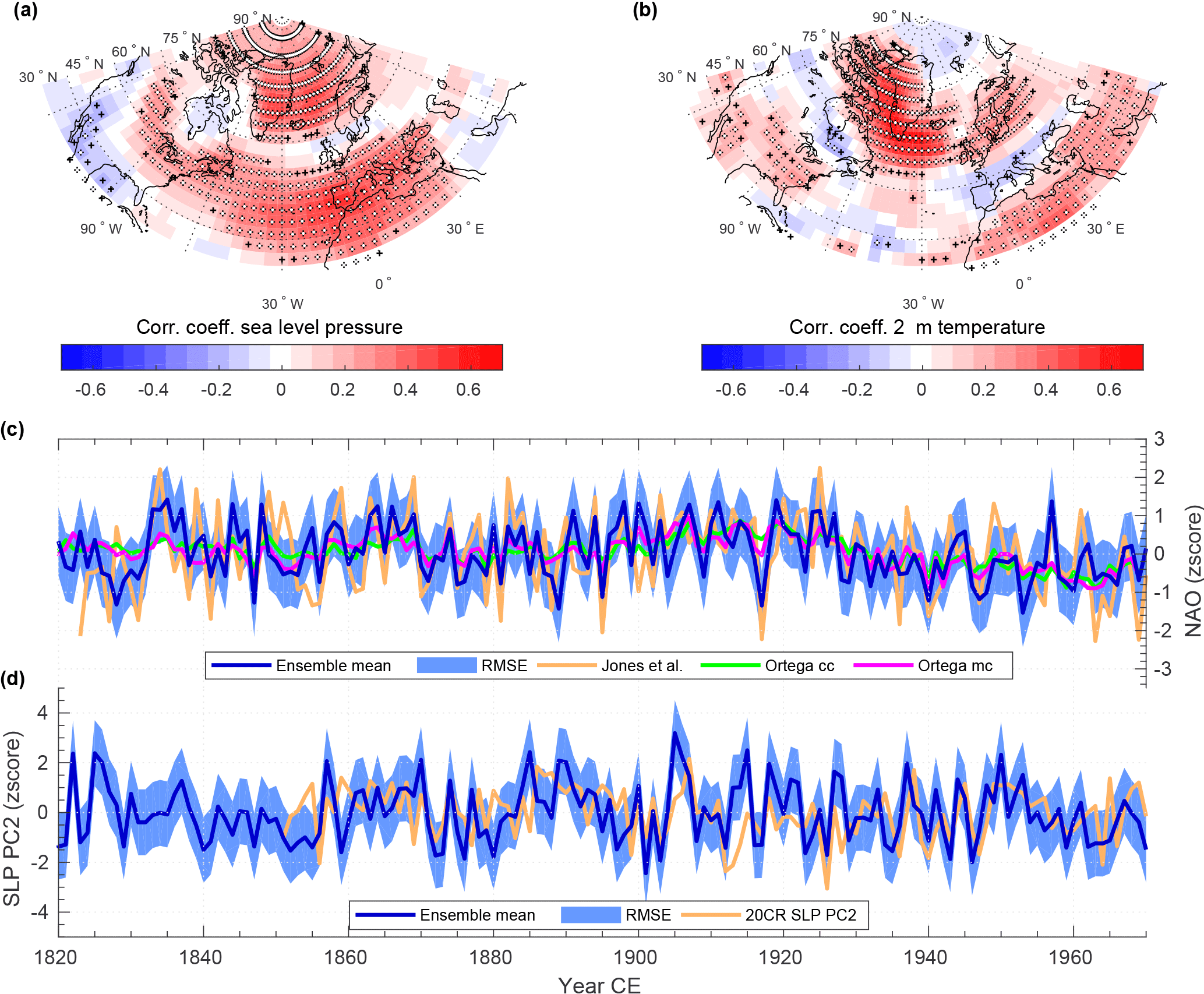
Figure 2Evaluation of the winter circulation reconstruction. Grid point correlation between reconstructed DJF SLP (a) and T2m (b), and reanalysis data (Compo et al., 2011) (1851–1970) interpolated to the model grid (lat. × long. ). The white stippling indicates significance p<0.05, and black stippling indicates significance p<0.1. (c) Ensemble mean reconstructed DJF NAO (PC1 of reconstructed DJF SLP Hurrell et al., 2003) with root mean square error (RMSE) compared to observed DJF NAO (Jones et al., 1997), NAOcc and NAOmc by Ortega et al. (2015). (d) Ensemble mean PC2 of reconstructed DJF SLP with RMSE compared to PC2 of reanalysis DJF SLP (Compo et al., 2011).
3.1 Evaluation of climate reconstruction
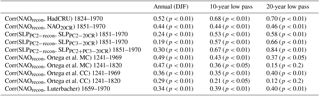
Comparing to the 20th Century Reanalysis (Compo et al., 2011; 20CR), our reconstruction shows skill for SLP and T2m in the North Atlantic region (Fig. 2a, b), the main mode of atmospheric circulation (NAO) as well as secondary circulation modes (Fig. 2c, d and Table 3). This is a completely independent test of the reconstruction as the reconstruction has not been calibrated to reanalysis data or observations. For T2m, the pattern of significant correlations with the 20CR data can be associated with the main circulation modes (Figs. S3 and S4), albeit with decreasing skill with the distance to the ice cores. We interpret the high skill near Greenland as being due to the direct physical connection between the local temperature in Greenland and the temperature along the path of the vapor, and the isotopic signal in Greenland ice cores. Contrary to previous millennial-scale reconstructions, our reconstructed NAO shows similar strength of year-to-year variability as the observed NAO indicating that the reconstruction preserves the known characteristic variability in the NAO (Figs. 2d, e and 3a). In addition to capturing the NAO, our reconstruction has skill in representing Atlantic ridge- or trough-type variability as projected on PC2 of SLP over the North Atlantic. The correlation of the reconstructed SLP PC2 and PC2 of the 20CR SLP is 0.24 (p<0.01) and increases to 0.53 (p<0.01) on decadal timescales (Table 3). However, comparing the SLP patterns of PC2 in our reconstruction and reanalysis (Fig. S3) implies that the variability captured by PC2 of the reconstruction is likely split between PC2 and PC3 in the reanalysis. Indeed, the reconstructed PC2 of SLP is also correlated to PC3 of the reanalysis SLP (, p<0.01, Table 3). Correlating the reconstructed PC2 of SLP against the sum of the reanalysis PC2 and PC3 shows increased correlations between the reconstruction and reanalysis, in particularly on decadal and bi-decadal timescales (Table 3). This indicates that the variability projected on PC2 and PC3 of the reanalysis data is partly summarized in PC2 of the reconstruction. The difference in distribution of the variability on the PCs in the reconstruction and reanalysis is likely due to (i) the intrinsic variability of the model used for the reconstruction and (ii) the reconstruction only capturing the North Atlantic variability as recorded in the isotopic composition of the Greenland ice core data.
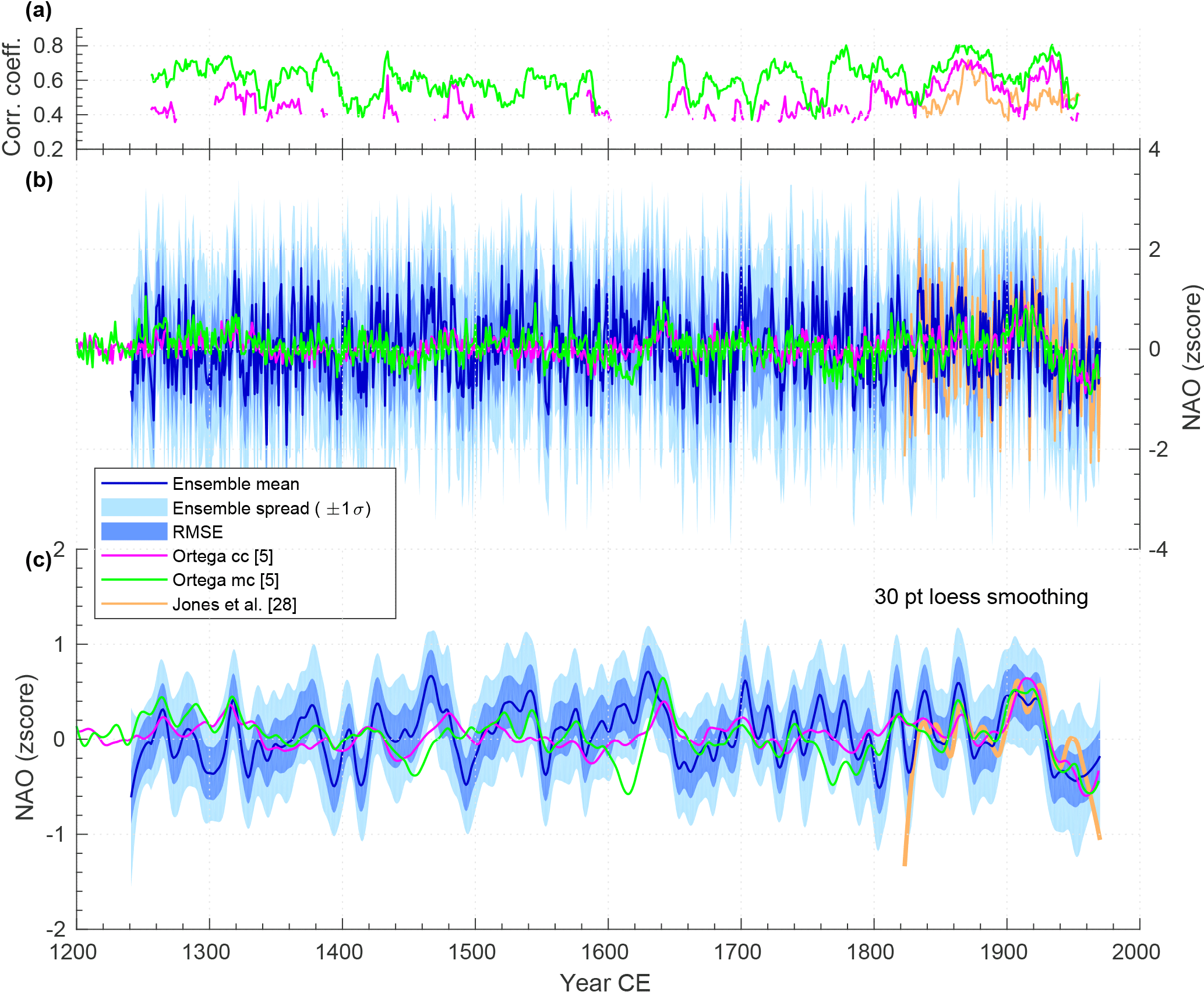
Figure 3Comparison of instrumental NAO and proxy-based NAO reconstructions. (a) Moving 31-point correlation between reconstructed NAO from this study and NAOcc (magenta), NAOmc (green; Ortega et al., 2015) and observed NAO (yellow; Jones et al., 1997). Only significant correlations are plotted (p<0.05). (a) Ensemble mean reconstructed NAO (PC1 of reconstructed SLP Hurrell et al., 2003) with error estimated by ensemble spread and RMSE, compared to observed NAO (Jones et al., 1997) and NAO reconstructions by Ortega et al. (2015). The amplitude of all time series are scaled to fit the decadal variability in the observed NAO. (c) Same as (b), except filtered with a 30 point “loess” filter.
Table 3Correlations of reconstructed NAO and PC2 of reconstructed SLP, and observed NAO, 20CR PC2 and PC3 of SLP, as well as NAO reconstructions by Ortega et al. (2015) and Luterbacher et al. (2004). All correlations are for detrended data, and p values are calculated with the random-phase test by Ebisuzaki (1997) to take into account autocorrelation.
The reconstructed NAO shows strong multidecadal variability, while no major trends are found on centennial timescales, as opposed to the reconstruction by Trouet et al. (2009), and in agreement with the NAO reconstructions by Ortega et al. (2015) (Fig. 3). The NAO reconstructions by Ortega et al. (2015) consists of two multi-proxy NAO reconstructions. Of these reconstructions, one is calibration-constrained (NAOcc) and the other model-constrained (NAOmc) (Fig. 3b), where NAOmc only uses proxies from sites that were estimated from model simulations to have a stable relation to the NAO. It should be noted that both the reconstruction by Ortega et al. (2015) and this study use some of the same Greenland ice core data (Crete, DYE-3, GRIP), which obviously could lead to a correspondence in variability. We find the NAO in our SLP reconstruction has best correspondence with NAOmc for interannual variability, while for multidecadal timescales prior to the instrumental period, there is little coherency between our reconstruction and both NAOmc and NAOcc (Table 3). This lack of coherence of multidecadal variability is similar to the aforementioned divergence between previous NAO reconstructions. For an independent comparison we used reconstructed NAO and gridded reconstructed SLP over Europe (Luterbacher et al., 2001), as well as gridded reconstructed temperature (Luterbacher et al., 2004) over Europe. However, we restricted the comparison to 1659–1970 due to the methodological differences in the reconstructions for Europe prior to and post-1659, and the use of Greenland ice core data for the European temperature reconstruction covering 1500–1658. For the NAO reconstruction by Luterbacher et al. (2001), our reconstruction shows slightly lower correlation on interannual timescales compared to the correlation to NAOmc, but similar correlation on decadal to multidecadal timescales (Table 3). The comparison between our reconstruction and these reconstructions for Europe shows similar pattern and correlation levels for SLP as with the 20CR data, and moderate, but significant, correlations for temperature (Fig. S5).
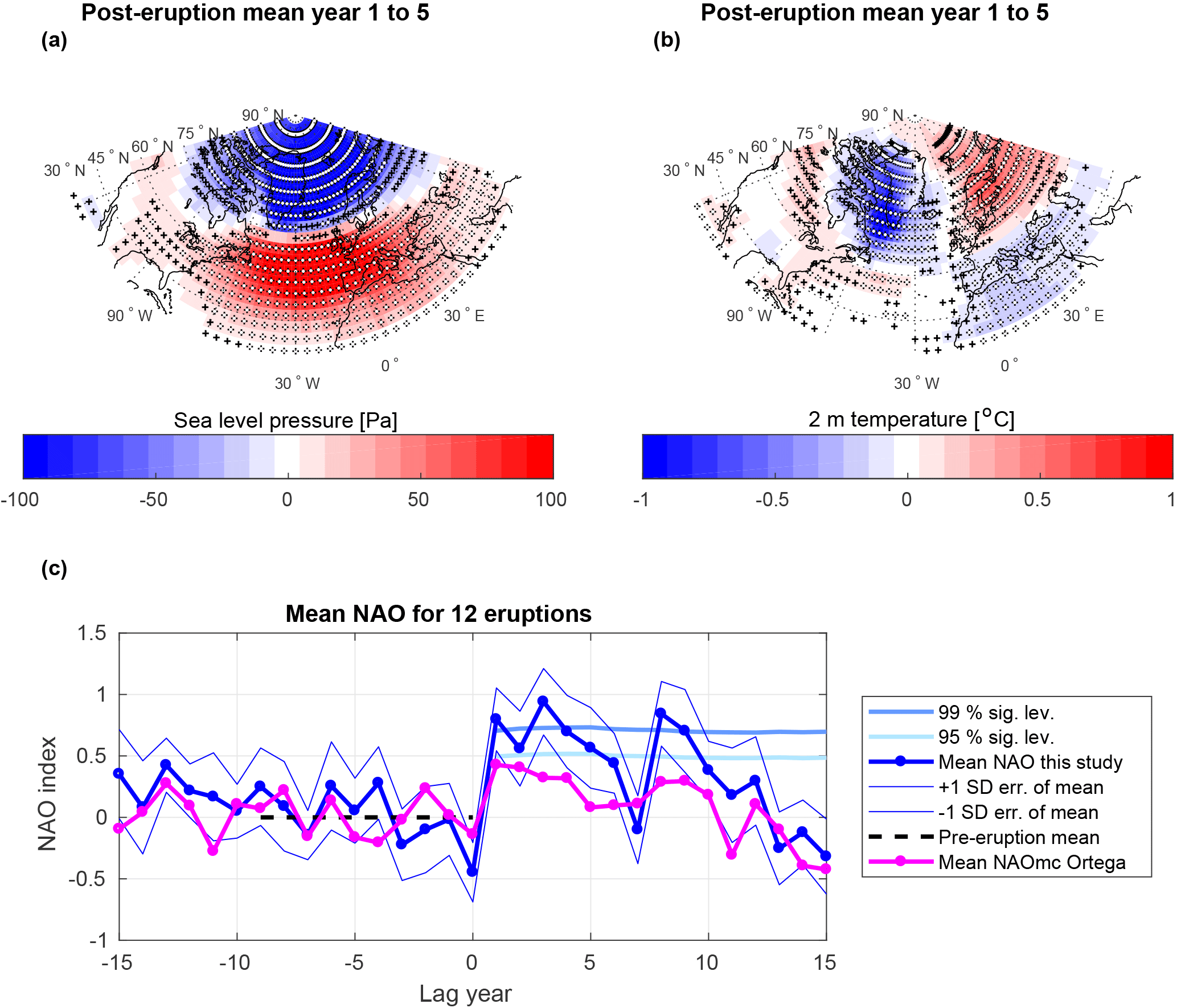
Figure 4Superimposed epoch analysis of the mean response in atmospheric circulation to the 12 largest tropical volcanic eruptions (Sigl et al., 2015; Table S1). The response in SLP and T2m is normalized to the mean fields of the 10 years preceding the eruption. (a) Mean DJF SLP anomalies (Pa) for the first five post-eruption years. (b) Mean DJF T2m anomalies (∘C) for the first five post-eruption years. The white stippling indicates significant anomalies p<0.01, and black stippling indicates significant anomalies p<0.05 (two-tailed Student's t test). (c) Mean response in reconstructed NAO (blue) with the time series normalized to the mean NAO of the 10 years preceding the eruption. For comparison the same analysis is carried out for the NAOmc reconstruction (magenta) by Ortega et al. (2015). The significance levels in (c) are estimated from 100 000 random samples of 12 years drawn from the reconstructed NAO. See Fig. S6 for significance levels for NAOmc.
Our reconstructed NAO shows higher correlation (, p<0.01) to the observed NAO (Jones et al., 1997) (DJF, 1824–1970) than NAOmc and NAOcc, which have correlations to the observed NAO of 0.46 and 0.47, respectively. Even more important, the skill of our reconstructed NAO is achieved without calibrating to the observed NAO. In summary, we think that our reconstruction is the most suitable for analyzing the influence of volcanic eruptions and solar activity on circulation, because (i) our reconstruction not only has good skill for the NAO but also for the secondary modes of circulation, which, as we will show later, is crucial for investigating the impact of solar forcing; (ii) high-frequency variability is preserved, making it possibly better to detect rapid shifts in circulation after volcanic eruptions; and finally (iii) our reconstruction is not calibrated to observed SLP or T2m, making it free of biases that could arise from tuning a reconstruction to observations during the instrumental era.
3.2 Response of atmospheric circulation to external forcing
In this section we investigate the reconstructed response in SLP and temperature to major tropical volcanic eruptions and solar variability. The mean post-eruption SLP and T2m anomalies in response to 12 major tropical eruptions show the characteristics of a positive NAO (Fig. 4a, b). On average, we find a significant positive NAO response during the five consecutive winters following the eruptions (Fig. 4c). Performing the same analysis on NAOmc yields a similar response, while not reaching as high significance levels and persistence as our reconstruction, likely due to the attenuated year-to-year variability in NAOmc (Figs. 2c, 4c and S6). Due to the short time span between some of the volcanic eruptions, it is not possible to consistently analyze any longer-term response than 5 years for single eruptions, since it would limit the number of eruptions and, hence, the robustness of the statistical analysis. We analyzed the decadal to multi-decadal response to volcanic forcing by calculating the correlation between reconstructed NAO and volcanic forcing from tropical eruptions (Toohey and Sigl, 2017) after filtering both data series with a band-pass filter. The correlation analysis of filtered data estimates the combined effect of the eruptions during the reconstructed time frame. Due to the very abrupt nature of the volcanic forcing, heavy filtering can introduce artificial forcing prior to the onset of the actual forcing. We find that smoothing the volcanic forcing data using a low-pass filter with no less than 1/10 cycle per year only has negligible effects on the analysis. Performing a time-lag correlation analysis on the band-pass filtered data (1/10 to 1/100 cycles per year) we obtain significant correlations (p<0.01) with the reconstructed NAO lagging the volcanic forcing 1 to 6 years (Fig. S7). This corresponds well to the results of the analysis of the mean NAO response for the 12 major tropical eruptions. Maximum correlation is reached at time lags of 3 to 4 years with a correlation of 0.33. This shows the cumulative effect of several volcanic eruptions which can cause trends in the NAO on longer timescales than single eruptions.
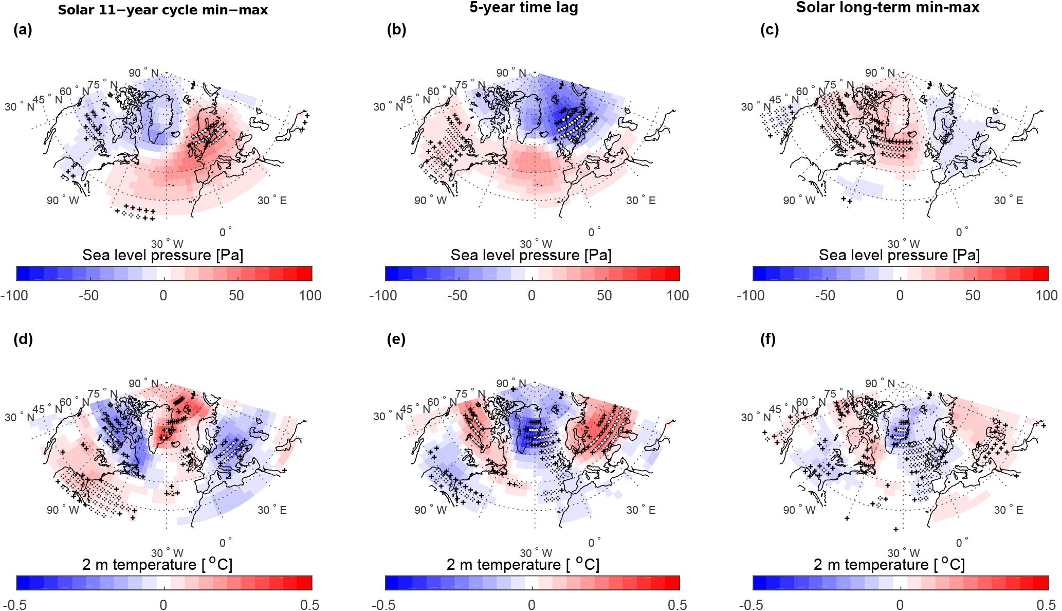
Figure 5Reconstructed atmospheric response to solar forcing. (a) DJF SLP anomalies (Pa) in response to the 11-year solar cycle (solar min. minus solar max. defined in Fig. S10). (b) DJF SLP anomalies (Pa) in response to the 5-year lagged 11-year solar cycle (solar min. minus solar max.). (c) DJF SLP anomalies (Pa) in response to the long-term solar forcing (solar min. minus solar max. defined in Fig. S11). (d, e, f) corresponding figures to (a, b, c), but for T2m (∘C). The white stippling indicates significant anomalies p<0.05, and black stippling indicates significant anomalies p<0.1 (two-tailed Student's t test).
For the analysis of solar influences on circulation, we analyzed the average response to the 11-year solar cycle and the multidecadal to centennial solar variability. We calculated the difference between reconstructed SLP and T2m for years of low and high solar activity using the annual sunspot number (Clette and Lefèvre, 2016; 1700–1970) and a 14C-based solar reconstruction (1241–1970; see Sect. 2.2) for the short-term and long-term cycles, respectively. The response to the 11-year solar cycle (solar low minus high) is a high pressure over Scandinavia corresponding well to the pattern found for reanalysis data (Figs. 5a, d and 6a, c). This anomalous high pressure could be due to increased frequency in Scandinavian blockings, which has been shown to impact Greenland δ18O (Ortega et al., 2014; Rimbu et al., 2017). Investigating the time-lagged response to the 11-year solar cycle, we find the strongest response in reconstructed SLP and T2m when lagging the solar forcing with 5 years, which also matches the time-lagged pattern found in reanalysis data (Figs. 5b, e and 6b, d). This pattern projects on PC2 of the reconstructed SLP, also with the strongest correlation between forcing and response when lagging the sunspot data by 5 years. Taking this time lag into account yields a consistent relationship between solar forcing and PC2 of reconstructed SLP on decadal to multidecadal timescales (Fig. 7, Table 4). The 5-year lagged response in circulation is not simply due to the response to the solar maximum approximately half a cycle later in the 11-year solar cycle, but a reinforced response. This is most clearly seen in the stronger correlations for the time-lagged response, both for the original data and the filtered data (Table 4, Figs. 7 and S8). The relation between PC2 of reconstructed SLP and solar forcing persists also for centennial variability, which is seen by comparing the circulation response to the 14C-based solar reconstruction (Table 4, Fig. S9). The pattern of the response in SLP to the long-term solar minima is an Atlantic ridge-type pattern (anomalous high south of Greenland), which also projects on PC2 of SLP, with an associated cooling pattern for the western North Atlantic (Fig. 5c, f). Compared to the 5-year lagged response to the 11-year cycle this pattern has the strongest response in SLP south of Greenland, with a similar, but more widespread cooling in the eastern North Atlantic. Even though the SLP response looks slightly different for short- and long-term solar forcing variations, the main feature, a wave structure over the North Atlantic and Scandinavia, is consistent (Fig. 5b, c). This similarity in the 5-year lagged and long-term response can also be seen in the patterns of the temperature anomalies (Fig. 5e, f). The temperature response to the long-term solar minima is a cooling across Greenland, Iceland and western Europe during solar minima (Fig. 5f). This cooling pattern corresponds well to the suggested cooling during the Little Ice Age in proxy records from Greenland (Stuiver et al., 1997), Iceland (Moffa-Sanchez et al., 2014) and Europe (Luterbacher et al., 2004). A NAO-type response to long-term solar forcing would give opposing temperature responses in Greenland and Europe, which is not the case. We find no consistent relation between our reconstructed NAO and solar forcing. Instead we would like to stress the importance of the connection between solar activity and the secondary circulation patterns, which possibly shows the main response to solar forcing on decadal to centennial timescales, with correlations of 0.29 (p<0.01) and 0.6 (p<0.01), respectively.
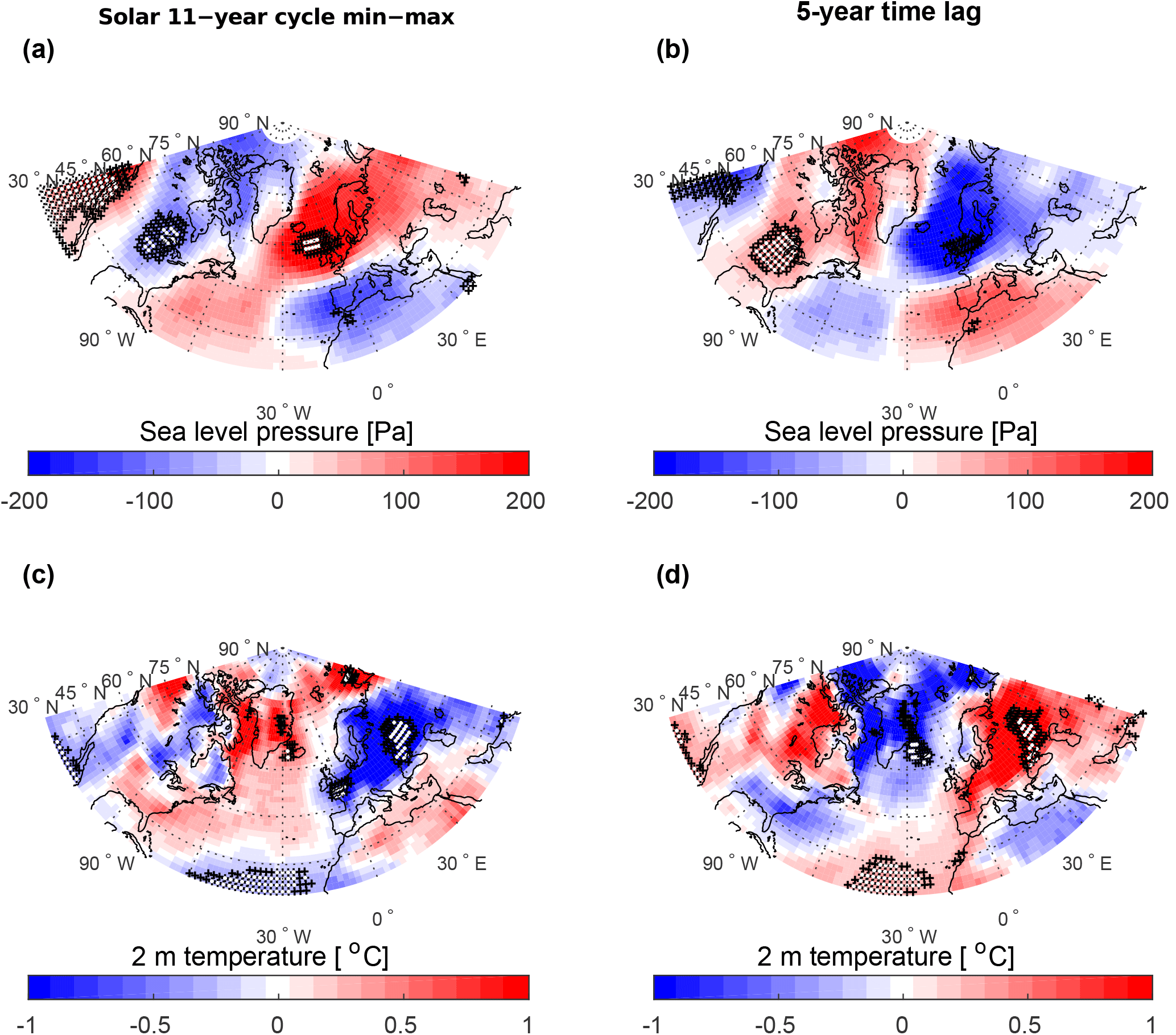
Figure 620CR (1948–2010) atmospheric response to solar forcing. (a) DJF SLP anomalies (Pa) in response to the 11-year solar cycle (solar min. minus solar max. defined in Fig. S12). (b) DJF SLP anomalies (Pa) in response to the 5-year lagged 11-year solar cycle (solar min. minus solar max.). (c, d) corresponding figures to (a, b), but for T2m (∘C). The white stippling indicates significant anomalies p<0.05, and black stippling indicates significant anomalies p<0.1 (two-tailed Student's t test). The time interval for this analysis in limited to 1948–2010 due to limitation of the data quality prior to this, although similar results can be achieved for the period 1851–2010.
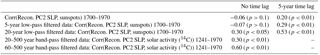
Table 4Correlation between solar forcing and PC2 of SLP, with and without time lag. The first column indicates which data are used, and if any filtering is done to the data. The second column is correlation coefficients between solar forcing and PC2 of reconstructed SLP, with solar forcing either being represented by sunspot number or 14C data. The third column is correlation coefficients between solar forcing and PC2 of reconstructed SLP, with solar forcing represented by sunspot number shifted for a lag of 5 years. All correlations are for detrended data, and p values are calculated with the random-phase test by Ebisuzaki (1997) to take into account autocorrelation.
The model simulation used for our reconstruction translates the climate variability recorded in the Greenland ice cores to climate variability in the North Atlantic region. In the initial test of the isotope variability, it is shown that the spatiotemporal δ18O variability in the ice cores is well represented by the model (Fig. 1). This is a fundamental prerequisite which allows us to match the modeled δ18O to the ice core δ18O year-by-year. While the skill of the reconstruction is higher in the vicinity around Greenland, the reconstruction shows significant correlations to reanalysis data wide spread across the North Atlantic region. This skill depends on (i) the integrative nature of the δ18O as recorded in the ice cores, and represented by the modeled δ18O; (ii) the modeled atmospheric teleconnection patterns in terms of temperature and circulation; and (iii) how these patterns are connected to modeled δ18O for Greenland. Clearly, the reconstruction is strongly dependent on the climate model when it comes to whether or not it is possible at all to use our method, and when it comes to the skill of reconstructed spatial patterns. The resolution of our model simulation is relatively course and using a higher-resolution simulation could improve the representation of several processes. For example, vapor transport to dry polar regions is often inhibited in models with courser resolution, resulting in too little precipitation in the interior of ice sheets and a positive bias in δ18O (Masson-Delmotte et al., 2008; Sjolte et al., 2011). This is related to cloud parameterizations and course-resolution models having difficulties in explicitly representing frontal zones in connection with synoptic weather systems. The orography in course-resolution models is also more smooth, loosing orographical features such as the southern dome of the Greenland ice sheet, which also affects atmospheric circulation and small-scale spatial variability. In our approach we match the modeled PCs of δ18O, meaning that we are matching regional-scale patterns in δ18O, which partly addresses the problem of matching course model output to site-specific proxy data. However, having a higher-resolution model simulation could for example improve the spatiotemporal representation of Greenland δ18O, allowing more than 3 PCs to be fitted, and generally giving a better representation of temperature, pressure and precipitation in the reconstruction. For reasons discussed above, it would be desirable using different GCMs to test for model dependencies of the reconstruction, as well as testing for added value of ensemble reconstructions with several different GCMs. Doing these tests is presently limited by the availability of millennium length simulations using isotope-enabled GCMs.
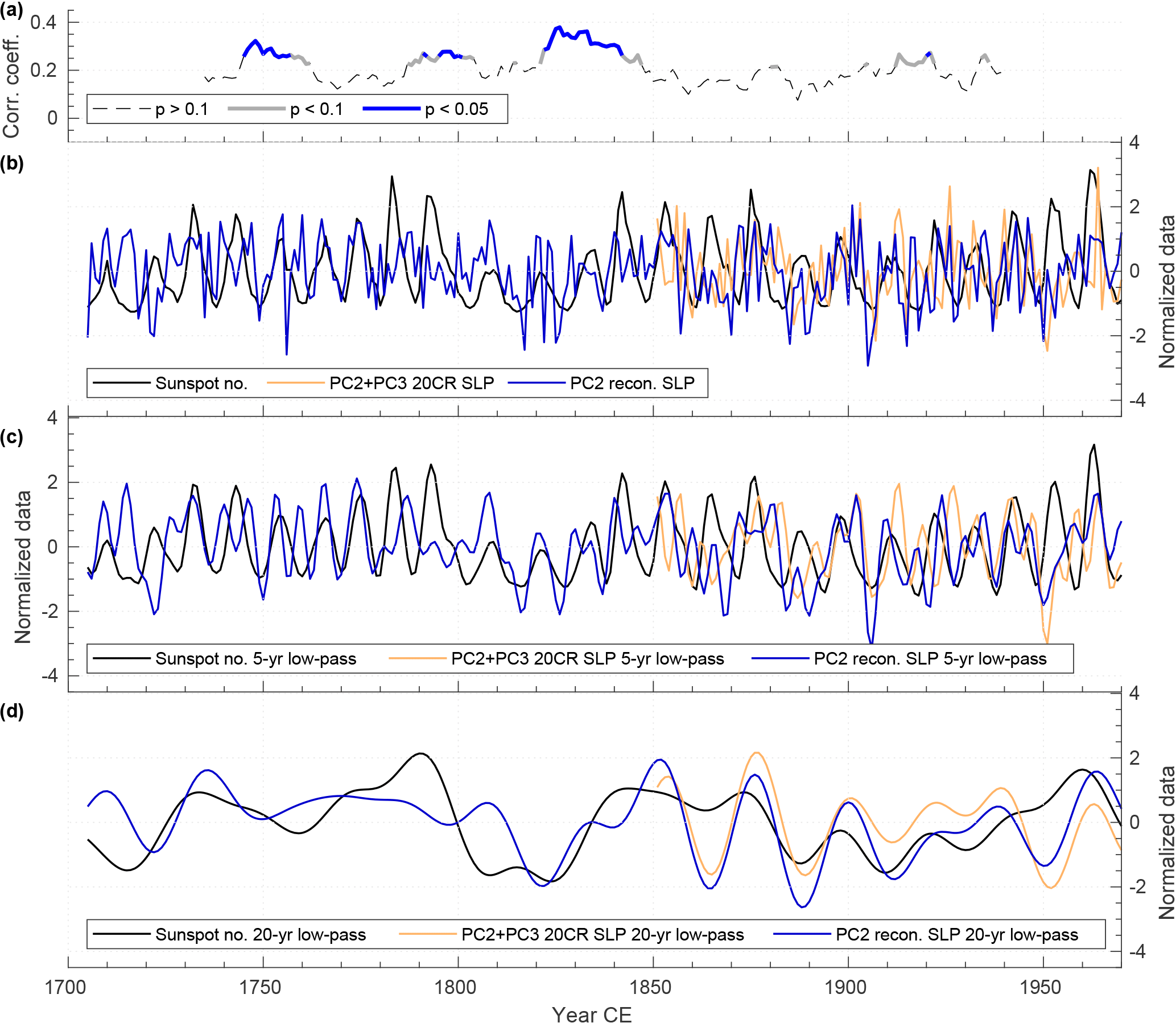
Figure 7Reconstructed PC2 of SLP plotted with the 5-year lagged sunspot number. (a) Moving 61-point correlation between reconstructed PC2 of SLP and sunspot number shifted for a 5-year time lag. (b) Time series of sunspot number shifted for a 5-year time lag, PC2+PC3 of 20CR SLP (see text and Table 4) and PC2 of reconstructed SLP. (c) Same as (b), except filtered with a 5-year low-pass filter. (d) Same as (b), except filtered with a 20-year low-pass filter.
We selected the proxy records for this study based on the criterion of having seasonal resolution, small dating uncertainty, a long time span and a wide regional spread. In order to provide a quantitative link to the isotope-enabled GCM we selected only isotope-based proxies. For the time being, this leaves us with the eight Greenland ice cores used in this study. Other seasonal resolution ice cores from Greenland are available, but only covering a limited time span, and comparing to these cores shows that the reconstructed δ18O also compares well to the isotopic variability at these sites (Fig. S2). However, including more Greenland ice cores of similar quality would generally improve the signal to noise ratio of the reconstruction, and such records should be included if available for subsequent studies. Obtaining seasonal resolution in ice core data is mainly limited by the accumulation rate and seasonality of precipitation, which depends on the regional climate setting of the drill site (Vinther et al., 2010; Zheng et al., 2018). Including other archives than ice cores would give a more widespread regional coverage, potentially providing better constraints on circulation patterns and climate trends. Some oxygen isotope records from tree rings in Sweden (e.g., Edwards et al., 2017) and speleothems from the European Alps (e.g., de Jong et al., 2013) covering the past millennium primarily reflect winter climate conditions. Both records in these examples have 5-year resolution, and the speleothem record has hiatuses, which reflect some of the challenges in using these proxy records. However, there could be benefits to using a larger selection of data, despite the different temporal resolution (Steiger and Hakim, 2016).
The comparison between the response to volcanic forcing between our reconstruction and NAOmc (Fig. 3c) shows that the mean response look qualitatively very similar in the two reconstructions. However, as already mentioned, due to the preserved high-frequency variability, our reconstruction shows both a more immediate and persistent NAO response to volcanoes. This underlines the importance of producing climate reconstructions that do preserve high-frequency variability, in particular if the reconstruction is used as baseline for model evaluation. In our analysis of the reconstructed response to volcanic eruptions we choose eruptions larger than or of similar magnitude to the 1991 Pinatubo eruption (). As discussed by Swingedouw et al. (2017), climate effects of smaller eruptions can be difficult to detect due to stochastic climate variability. We find that we can detect an impact on reconstructed NAO from tropical eruptions selected in the range from −4 to (Sigl et al., 2015), yielding a significant positive NAO 1 year after the eruptions, on average. This appears to be the limit of detection for our reconstruction, possibly owing both to the partly stochastic variability in the NAO and to noise in the reconstruction.
Model studies of the volcanic response to major tropical eruptions during the past millennium show a large spread in the modeled NAO response, with either no consistent response or 1–2 years of significant response (Swingedouw et al., 2017; Zambri et al., 2017). In contrast to this we find a clear tendency for positive NAO for the five consecutive winters following the year of eruption as an average response to the 12 largest tropical eruptions during 1241–1970 CE. An immediate strengthening of the polar vortex following eruptions is in agreement with the observed response of atmospheric circulation (Driscoll et al., 2012), which then translates to a positive NAO as the stratospheric anomaly propagates to the troposphere. The presence of volcanic aerosols gradually tails off during the first 2–3 years (Crowley and Unterman, 2013) and a more sustained positive NAO for up to 5 years could be explained via a positive ocean feedback through a tri-pole sea surface temperature (SST) response to the strongly anomalous positive NAO (Cayan, 1992). Ongoing efforts to improve the simulation of volcanic forcing and response could help close the gap between models and observations as well as reconstructions (Zanchettin et al., 2016).
It has been suggested that the observed increase in blocking frequency over the North Atlantic in response to solar minima (Woollings et al., 2010) is coupled to a weakening of the polar night jet in response to a weaker stratospheric equator–pole temperature gradient. This mechanism could be in play on both decadal and centennial timescales. A recent study investigated the response of circulation to solar activity using a regression-based analysis between sunspot data and gridded observed SLP and SST data (Gray et al., 2016). The authors analyzed the time-lagged response to solar forcing, and found that the solar response could be explained via two mechanisms (Gray et al., 2016). One involving the aforementioned stratosphere–troposphere coupling acting on time lags of 0–2 years, and one for time lags of 3–4 years involving ocean temperature anomalies being stored beneath the mixed layer and reinforced from the previous winter (Gray et al., 2016). The reinforcement of SST anomalies from year-to-year has also been shown in a simulation of the response to the solar 11-year cycle (Andrews et al., 2015). Such a mechanism could be the cause of the time lag we see in the reconstructed response to solar forcing, although we get the maximum response at 5-year time lag, compared to the 3–4 year time lag found in observations (Gray et al., 2016). However, this difference could be due to differences in the methodologies of the analysis of the response to solar forcing, and that the aforementioned study (Gray et al., 2016) is focusing on the NAO-like response seen in their analysis. A possible mechanism based on our findings is as follows. An initial increase in atmospheric blockings weakens the subpolar gyre (SPG; Moffa-Sanchez et al., 2014) , thereby decreasing the heat transport to the north-western North Atlantic giving favorable conditions for mid-Atlantic blocking. This pattern is reinforced year-by-year and the main atmospheric response shifts to the node of PC2 of SLP south of Greenland under sustained forcing conditions on longer timescales (Fig. 5c). A recent model study (Moreno-Chamarro et al., 2017) suggested that the cooling during the Little Ice Age was connected to a weakening in the SPG, sustained by way of atmosphere–ocean feedbacks. Although the authors do not relate this to solar forcing, but with preconditioned initial model variability, the anomalies in SLP and temperature associated with the weakening of the SPG are very similar to the reconstructed pattern of the response to long-term solar forcing. One explanation could be that low solar activity is the preconditioning factor in reality, causing the response to solar forcing seen in our reconstruction, while the climate response to solar forcing might not be fully captured by the MPI-ESM (Mitchell et al., 2015) used by Moreno-Chamarro et al. (2017). Our study of the reconstructed North Atlantic winter circulation shows a complex response to solar forcing which is, in contrast to a prevalent hypothesis, not directly linked to the NAO. The complexity is also reflected in a nonuniform temperature response to solar forcing, with both regional warming and cooling. This also means that part of this signal will be smoothed out if such analysis is carried out on hemispherical mean temperature (e.g., Schurer et al., 2015). In our study we do not exclude that there could be an influence of the solar 11-year cycle on NAO. However, unlike for PC2 of reconstructed SLP, we find no consistent relationship between reconstructed NAO and solar forcing across multiple timescales. Furthermore, the results suggest that sustained longer-term solar forcing leads to a shift in the atmospheric circulation response compared to the response to the short-term forcing, possibly due to feedback processes involving the ocean integrating the long-term effects of anomalous atmospheric circulation.
Our study presents a new climate reconstruction of SLP and temperature for the North Atlantic region. The reconstruction not only resolves the first mode of atmospheric circulation (PC1), the NAO, but also captures the second mode (PC2), referred to as the Eastern Atlantic Pattern. In the analysis of our reconstruction we find that solar and volcanic forcing impacts different modes of the atmospheric circulation during winter, which can aid to separate the regional effects of forcings and understand the underlying mechanisms. The reconstructed response to forcings can also serve as a baseline for climate model evaluation. Although atmospheric variability to a large extent is a stochastic process, the variability in our reconstruction also shows an overall significant impact of forcings. The squared correlation coefficient can provide an estimate for explained variance in the external forcings. Using this approach, tropical volcanic forcing accounts for about 10 % of the decadal to multidecadal variability in the reconstructed NAO, while solar forcing accounts for about 40 % of the variability in PC2 of reconstructed SLP on centennial timescales.
The time series of PC1 and PC2 of reconstructed SLP in the North Atlantic region are available at the PANGAEA open-access data library (https://doi.pangaea.de/10.1594/PANGAEA.892841, Sjolte, 2018). To obtain the complete climate field reconstructions of SLP and T2m, or the ECHAM5/MPI-OM simulation, please contact the corresponding author.
The supplement related to this article is available online at: https://doi.org/10.5194/cp-14-1179-2018-supplement.
JS developed the method, performed the analysis, conducted the model simulation and wrote the first version of the manuscript. CS initiated the study and contributed to setting up the model simulation. FA contributed to the method development and analysis. BV provided seasonal ice core data. MW provided technical support for model simulation and access to climate model. GL provided insights into model setup. RM contributed with solar activity reconstruction and provided insight into the solar forcing of climate. All authors discussed and edited the manuscript.
The authors declare that they have no conflict of interest.
This work was supported by the Swedish Research Council (grant DNR2011-5418
& DNR2013-8421 to Raimund Muscheler), the Crafoord foundation and the
strategic research program of ModEling the Regional and Global Earth system
(MERGE) hosted by the Faculty of Science at Lund University. The model
simulation was carried out at the AWI Computer and Data Center,
Bremerhaven.
Edited by: Marit-Solveig
Seidenkrantz
Reviewed by: two anonymous referees
Adolphi, F., Muscheler, R., Svensson, A., Aldahan, A., Possnert, G., Beer, J., Sjolte, J., Bjorck, S., Matthes, K., and Thieblemont, R.: Persistent link between solar activity and Greenland climate during the Last Glacial Maximum, Nat. Geosci., 7, 662–666, https://doi.org/10.1038/NGEO2225, 2014. a, b
Andrews, M. B., Knight, J. R., and Gray, L. J.: A simulated lagged response of the North Atlantic Oscillation to the solar cycle over the period 1960–2009, Environ. Res. Lett., 10, 054022, https://doi.org/10.1088/1748-9326/10/5/054022, 2015. a
Bond, G., Kromer, B., Beer, J., Muscheler, R., Evans, M., Showers, W., Hoffmann, S., Lotti-Bond, R., Hajdas, I., and Bonani, G.: Persistent solar influence on north Atlantic climate during the Holocene, Science, 294, 2130–2136, https://doi.org/10.1126/science.1065680, 2001. a
Bretagnon, P. and Francou, G.: Planetary theories in rectangular and spherical variables – vsop-87 solutions, Astron. Astrophys., 202, 309–315, 1988. a
Cayan, D. R.: Latent and sensible heat-flux anomalies over the northern oceans – Driving the sea-surface temperature, J. Phys. Oceanogr., 22, 859–881, https://doi.org/10.1175/1520-0485(1992)022<0859:LASHFA>2.0.CO;2, 1992. a
Clette, F. and Lefèvre, L.: The New Sunspot Number: Assembling All Corrections, Sol. Phys., 291, 2629–2651, https://doi.org/10.1007/s11207-016-1014-y, 2016. a
Compo, G. P., Whitaker, J. S., Sardeshmukh, P. D., Matsui, N., Allan, R. J., Yin, X., Gleason, Jr., B. E., Vose, R. S., Rutledge, G., Bessemoulin, P., Broennimann, S., Brunet, M., Crouthamel, R. I., Grant, A. N., Groisman, P. Y., Jones, P. D., Kruk, M. C., Kruger, A. C., Marshall, G. J., Maugeri, M., Mok, H. Y., Nordli, O., Ross, T. F., Trigo, R. M., Wang, X. L., Woodruff, S. D., and Worley, S. J.: The Twentieth Century Reanalysis Project, Q. J. Roy. Meteor. Soc., 137, 1–28, https://doi.org/10.1002/qj.776, 2011. a, b, c, d
Crowley, T. J. and Unterman, M. B.: Technical details concerning development of a 1200 yr proxy index for global volcanism, Earth Syst. Sci. Data, 5, 187–197, https://doi.org/10.5194/essd-5-187-2013, 2013. a
Crowley, T. J., Zielinski, G., Vinther, B., Udisti, R., Kreutz, K., Cole-Dai, J., and Castellano, J.: Volcanism and the Little Ice Age, PAGES Newsletter, 16, 22–23, 2008. a
de Jong, R., Kamenik, C., and Grosjean, M.: Cold-season temperatures in the European Alps during the past millennium: variability, seasonality and recent trends, Quaternary Sci. Rev., 82, 1–12, https://doi.org/10.1016/j.quascirev.2013.10.007, 2013. a
Driscoll, S., Bozzo, A., Gray, L. J., Robock, A., and Stenchikov, G.: Coupled Model Intercomparison Project 5 (CMIP5) simulations of climate following volcanic eruptions, J. Geophys. Res.-Atmos., 117, D17105, https://doi.org/10.1029/2012JD017607, 2012. a, b
Ebisuzaki, W.: A method to estimate the statistical significance of a correlation when the data are serially correlated, J. Climate, 10, 2147–2153, https://doi.org/10.1175/1520-0442(1997)010<2147:AMTETS>2.0.CO;2, 1997. a, b, c
Edwards, T. W., Hammarlund, D., Newton, B. W., Sjolte, J., Linderson, H., Sturm, C., Amour, N. A. S., Bailey, J. N.-L., and Nilsson, A. L.: Seasonal variability in Northern Hemisphere atmospheric circulation during the Medieval Climate Anomaly and the Little Ice Age, Quaternary Sci. Rev., 165, 102–110, https://doi.org/10.1016/j.quascirev.2017.04.018, 2017. a
Gray, L. J., Scaife, A. A., Mitchell, D. M., Osprey, S., Ineson, S., Hardiman, S., Butchart, N., Knight, J., Sutton, R., and Kodera, K.: A lagged response to the 11 year solar cycle in observed winter Atlantic/European weather patterns, J. Geophys. Res.-Atmos., 118, 13405–13420, https://doi.org/10.1002/2013JD020062, 2013. a, b
Gray, L. J., Woollings, T. J., Andrews, M., and Knight, J.: Eleven-year solar cycle signal in the NAO and Atlantic/European blocking, Q. J. Roy. Meteor. Soc., 142, 1890–1903, https://doi.org/10.1002/qj.2782, 2016. a, b, c, d, e
Haigh, J. D. and Blackburn, M.: Solar influences on dynamical coupling between the stratosphere and troposphere, Space Sci. Rev., 125, 331–344, https://doi.org/10.1007/s11214-006-9067-0, 2006. a
Hakim, G. J., Emile-Geay, J., Steig, E. J., Noone, D., Anderson, D. M., Tardif, R., Steiger, N., and Perkins, W. A.: The lastmillennium climate reanalysis project: Framework and first results, J. Geophys. Res.-Atmos., 121, 6745–6764, https://doi.org/10.1002/2016JD024751, 2016. a
Hurrell, J. W., Kushnir, Y., Visbeck, M., and Ottersen, G. (Eds.): An overview of the North Atlantic Oscillation, in: The North Atlantic Oscillation, Climatic Significance and Environmental Impact, AGU Geophysical Monograph, 134, 1–35, American Geophysics Union, Washington, DC, 2003. a, b, c, d, e, f
Ineson, S., Scaife, A. A., Knight, J. R., Manners, J. C., Dunstone, N. J., Gray, L. J., and Haigh, J. D.: Solar forcing of winter climate variability in the Northern Hemisphere, Nat. Geosci., 4, 753–757, https://doi.org/10.1038/NGEO1282, 2011. a
Jiang, H., Muscheler, R., Bjorck, S., Seidenkrantz, M.-S., Olsen, J., Sha, L., Sjolte, J., Eiriksson, J., Ran, L., Knudsen, K.-L., and Knudsen, M. F.: Solar forcing of Holocene summer sea-surface temperatures in the northern North Atlantic, Geology, 43, 203–206, https://doi.org/10.1130/G36377.1, 2015. a
Johnsen, S. and Vinther, B.: Ice Core Records Greenland Stable Isotopes, in: Encyclopedia of Quaternary Science, edited by: Elias, S. A., 1250–1258, Elsevier, Oxford, https://doi.org/10.1016/B0-44-452747-8/00345-8, 2007. a
Jones, P., Jonsson, T., and Wheeler, D.: Extension to the North Atlantic Oscillation using early instrumental pressure observations from Gibraltar and south-west Iceland, Int. J. Climatol., 17, 1433–1450, https://doi.org/10.1002/(SICI)1097-0088(19971115)17:13<1433::AID-JOC203>3.0.CO;2-P, 1997. a, b, c, d
Jungclaus, J. H., Lorenz, S. J., Timmreck, C., Reick, C. H., Brovkin, V., Six, K., Segschneider, J., Giorgetta, M. A., Crowley, T. J., Pongratz, J., Krivova, N. A., Vieira, L. E., Solanki, S. K., Klocke, D., Botzet, M., Esch, M., Gayler, V., Haak, H., Raddatz, T. J., Roeckner, E., Schnur, R., Widmann, H., Claussen, M., Stevens, B., and Marotzke, J.: Climate and carbon-cycle variability over the last millennium, Clim. Past, 6, 723–737, https://doi.org/10.5194/cp-6-723-2010, 2010. a, b
Jungclaus, J. H., Bard, E., Baroni, M., Braconnot, P., Cao, J., Chini, L. P., Egorova, T., Evans, M., González-Rouco, J. F., Goosse, H., Hurtt, G. C., Joos, F., Kaplan, J. O., Khodri, M., Klein Goldewijk, K., Krivova, N., LeGrande, A. N., Lorenz, S. J., Luterbacher, J., Man, W., Maycock, A. C., Meinshausen, M., Moberg, A., Muscheler, R., Nehrbass-Ahles, C., Otto-Bliesner, B. I., Phipps, S. J., Pongratz, J., Rozanov, E., Schmidt, G. A., Schmidt, H., Schmutz, W., Schurer, A., Shapiro, A. I., Sigl, M., Smerdon, J. E., Solanki, S. K., Timmreck, C., Toohey, M., Usoskin, I. G., Wagner, S., Wu, C.-J., Yeo, K. L., Zanchettin, D., Zhang, Q., and Zorita, E.: The PMIP4 contribution to CMIP6 – Part 3: The last millennium, scientific objective, and experimental design for the PMIP4 past1000 simulations, Geosci. Model Dev., 10, 4005–4033, https://doi.org/10.5194/gmd-10-4005-2017, 2017. a
Kodera, K. and Kuroda, Y.: A possible mechanism of solar modulation of the spatial structure of the North Atlantic Oscillation, J. Geophys. Res.-Atmos., 110, d02111, https://doi.org/10.1029/2004JD005258, 2005. a
Lefohn, A., Husar, J., and Husar, R.: Estimating historical anthropogenic global sulfur emission patterns for the period 1850-1990, Atmos. Environ., 33, 3435–3444, https://doi.org/10.1016/S1352-2310(99)00112-0, 214th National Meeting of the American-Chemical-Society, Las Vegas, Nevada, 07–11 September, 1997, 1999. a
Luterbacher, J., Xoplaki, E., Dietrich, D., Jones, P. D., Davies, T. D., Portis, D., Gonzalez-Rouco, J. F., von Storch, H., Gyalistras, D., Casty, C., and Wanner, H.: Extending North Atlantic oscillation reconstructions back to 1500, Atmos. Sci. Lett., 2, 114–124, https://doi.org/10.1006/asle.2002.0047, 2001. a, b
Luterbacher, J., Dietrich, D., Xoplaki, E., Grosjean, M., and Wanner, H.: European seasonal and annual temperature variability, trends, and extremes since 1500, Science, 303, 1499–1503, https://doi.org/10.1126/science.1093877, 2004. a, b, c
MacFarling Meure, C., Etheridge, D., Trudinger, C., Steele, P., Langenfelds, R., van Ommen, T., Smith, A., and Elkins, J.: Law Dome CO2, CH4 and N2O ice core records extended to 2000 years BP, Geophys. Res. Lett., 33, L14810, https://doi.org/10.1029/2006GL026152, 2006. a
Marland, G., Boden, T. A., and Andres, R. J.: Global, regional and national emissions, in: Trends: a compendium of data on global change, Carbon Dioxide Information Center, Oak Ridge National Laboratory, US Department of Energy, Oak Ridge, TN, 2003. a
Masson-Delmotte, V., Hou, S., Ekaykin, A., Jouzel, J., Aristarain, A., Bernardo, R. T., Bromwich, D., Cattani, O., Delmotte, M., Falourd, S., Frezzotti, M., Gallée, H., Genoni, L., Isaksson, E., Landais, A., Helsen, M. M., Hoffmann, G., Lopez, J., Morgan, V., Motoyama, H., Noone, D., Oerter, H., Petit, J. R., Royer, A., Uemura, R., Schmidt, G. A., Schlosser, E., Simões, J. C., Steig, E. J., Stenni, B., Stievenard, M., van den Broeke, M. R., van de Wal, R. S. W., van de Berg, W. J., Vimeux, F., and White, J. W. C.: A Review of Antarctic Surface Snow Isotopic Composition: Observations, Atmospheric Circulation, and Isotopic Modeling, J. Climate, 21, 3359–3387, https://doi.org/10.1175/2007JCLI2139.1, 2008. a
Mitchell, D. M., Misios, S., Gray, L. J., Tourpali, K., Matthes, K., Hood, L., Schmidt, H., Chiodo, G., Thiéblemont, R., Rozanov, E., Shindell, D., and Krivolutsky, A.: Solar signals in CMIP-5 simulations: the stratospheric pathway, Q. J. Roy. Meteor. Soc., 141, 2390–2403, https://doi.org/10.1002/qj.2530, 2015. a
Moffa-Sanchez, P., Born, A., Hall, I. R., Thornalley, D. J. R., and Barker, S.: Solar forcing of North Atlantic surface temperature and salinity over the past millennium, Nat. Geosci., 7, 275–278, https://doi.org/10.1038/ngeo2094, 2014. a, b, c
Moreno-Chamarro, E., Zanchettin, D., Lohmann, K., and Jungclaus, J. H.: An abrupt weakening of the subpolar gyre as trigger of Little Ice Age-type episodes, Clim. Dynam., 48, 727–744, https://doi.org/10.1007/s00382-016-3106-7, 2017. a, b
Muscheler, R., Joos, F., Beer, J., Müller, S. A., Vonmoos, M., and Snowball, I.: Solar activity during the last 1000 yr inferred from radionuclide records, Quaternary Sci. Rev., 26, 82–97, https://doi.org/10.1016/j.quascirev.2006.07.012, 2007. a, b
Muscheler, R., Adolphi, F., Herbst, K., and Nilsson, A.: The Revised Sunspot Record in Comparison to Cosmogenic Radionuclide-Based Solar Activity Reconstructions, Sol. Phys., 291, 3025–3043, https://doi.org/10.1007/s11207-016-0969-z, 2016. a, b
Ortega, P., Swingedouw, D., Masson-Delmotte, V., Risi, C., Vinther, B., Yiou, P., Vautard, R., and Yoshimura, K.: Characterizing atmospheric circulation signals in Greenland ice cores: insights from a weather regime approach, Clim. Dynam., 43, 2585–2605, https://doi.org/10.1007/s00382-014-2074-z, 2014. a
Ortega, P., Lehner, F., Swingedouw, D., Masson-Delmotte, V., Raible, C. C., Casado, M., and Yiou, P.: A model-tested North Atlantic Oscillation reconstruction for the past millennium, Nat., 523, 71–74, https://doi.org/10.1038/nature14518, 2015. a, b, c, d, e, f, g, h, i, j
Paul, J., Fortuin, F., and Kelder, H.: An ozone climatology based on ozonesonde and satellite measurements, J. Geophys. Res.-Atmos., 103, 31709–31734, https://doi.org/10.1029/1998JD200008, 1998. a
Pinto, J. G. and Raible, C. C.: Past and recent changes in the North Atlantic oscillation, Wires Clim. Change, 3, 79–90, https://doi.org/10.1002/wcc.150, 2012. a
Pongratz, J., Reick, C., Raddatz, T., and Claussen, M.: A reconstruction of global agricultural areas and land cover for the last millennium, Global Biogeochem. Cy., 22, GB3018, https://doi.org/10.1029/2007GB003153, 2008. a
Rimbu, N., Lohmann, G., Werner, M., and Ionita, M.: Links between central Greenland stable isotopes, blocking and extreme climate variability over Europe at decadal to multidecadal time scales, Clim. Dynam., 49, 649–663, https://doi.org/10.1007/s00382-016-3365-3, 2017. a
Scaife, A. A., Ineson, S., Knight, J. R., Gray, L., Kodera, K., and Smith, D. M.: A mechanism for lagged North Atlantic climate response to solar variability, Geophys. Res. Lett., 40, 434–439, https://doi.org/10.1002/grl.50099, 2013. a
Schmidt, G. A., Jungclaus, J. H., Ammann, C. M., Bard, E., Braconnot, P., Crowley, T. J., Delaygue, G., Joos, F., Krivova, N. A., Muscheler, R., Otto-Bliesner, B. L., Pongratz, J., Shindell, D. T., Solanki, S. K., Steinhilber, F., and Vieira, L. E. A.: Climate forcing reconstructions for use in PMIP simulations of the last millennium (v1.0), Geosci. Model Dev., 4, 33–45, https://doi.org/10.5194/gmd-4-33-2011, 2011. a, b, c, d, e
Schmidt, G. A., Jungclaus, J. H., Ammann, C. M., Bard, E., Braconnot, P., Crowley, T. J., Delaygue, G., Joos, F., Krivova, N. A., Muscheler, R., Otto-Bliesner, B. L., Pongratz, J., Shindell, D. T., Solanki, S. K., Steinhilber, F., and Vieira, L. E. A.: Climate forcing reconstructions for use in PMIP simulations of the Last Millennium (v1.1), Geosci. Model Dev., 5, 185–191, https://doi.org/10.5194/gmd-5-185-2012, 2012. a, b, c
Schurer, A. P., Tett, S. F. B., and Hegerl, G. C.: Small influence of solar variability on climate over the past millennium (vol 7, pg 104, 2014), Nat. Geosci., 8, 159, https://doi.org/10.1038/NGEO2342, 2015. a
Sejrup, H. P., Lehman, S. J., Haflidason, H., Noone, D., Muscheler, R., Berstad, I. M., and Andrews, J. T.: Response of Norwegian Sea temperature to solar forcing since 1000 A.D., J. Geophys. Res.-Oceans, 115, c12034, https://doi.org/10.1029/2010JC006264, 2010. a
Shindell, D. T., Schmidt, G. A., Mann, M. E., Rind, D., and Waple, A.: Solar Forcing of Regional Climate Change During the Maunder Minimum, Science, 294, 2149–2152, https://doi.org/10.1126/science.1064363, 2001. a
Sigl, M., Winstrup, M., McConnell, J. R., Welten, K. C., Plunkett, G., Ludlow, F., Buentgen, U., Caffee, M., Chellman, N., Dahl-Jensen, D., Fischer, H., Kipfstuhl, S., Kostick, C., Maselli, O. J., Mekhaldi, F., Mulvaney, R., Muscheler, R., Pasteris, D. R., Pilcher, J. R., Salzer, M., Schuepbach, S., Steffensen, J. P., Vinther, B. M., and Woodruff, T. E.: Timing and climate forcing of volcanic eruptions for the past 2,500 years, Nature, 523, 543–549, https://doi.org/10.1038/nature14565, 2015. a, b, c
Sjolte, J.: Reconstructed main atmospheric circulation modes during winter in the North Atlantic region covering 1241–1970 CE, based on Greenland ice cores and an isotope enabled climate model simulation, PANGAEA, https://doi.org/10.1594/PANGAEA.892841, 2018. a
Sjolte, J., Hoffmann, G., Johnsen, S. J., Vinther, B. M., Masson-Delmotte, V., and Sturm, C.: Modeling the water isotopes in Greenland precipitation 1959–2001 with the meso-scale model REMO-iso, J. Geophys. Res.-Atmos., 116, D18105, https://doi.org/10.1029/2010JD015287, 2011. a
Steiger, N. and Hakim, G.: Multi-timescale data assimilation for atmosphere-ocean state estimates, Clim. Past, 12, 1375–1388, https://doi.org/10.5194/cp-12-1375-2016, 2016. a
Steiger, N. J., Steig, E. J., Dee, S. G., Roe, G. H., and Hakim, G. J.: Climate reconstruction using data assimilation of water isotope ratios from ice cores, J. Geophys. Res.-Atmos., 122, 1545–1568, https://doi.org/10.1002/2016JD026011, 2017. a
Stuiver, M., Braziunas, T., Grootes, P., and Zielinski, G.: Is There Evidence for Solar Forcing of Climate in the GISP2 Oxygen Isotope Record?, Quaternary Res., 48, 259–266, https://doi.org/10.1006/qres.1997.1931, 1997. a
Swingedouw, D., Terray, L., Cassou, C., Voldoire, A., Salas-Mélia, D., and Servonnat, J.: Natural forcing of climate during the last millennium: fingerprint of solar variability, Clim. Dynam., 36, 1349–1364, https://doi.org/10.1007/s00382-010-0803-5, 2011. a
Swingedouw, D., Mignot, J., Ortega, P., Khodri, M., Menegoz, M., Cassou, C., and Hanquiez, V.: Impact of explosive volcanic eruptions on the main climate variability modes, Global Planet. Change, 150, 24–45, https://doi.org/10.1016/j.gloplacha.2017.01.006, 2017. a, b, c
Tanre, D., Geleyn, J.-F., and Slingo, J. M.: Aerosols and Their Climatic Effects, chap. First results of the introduction of an advanced aerosol-radiation interaction in the ECMWF low resolution global model, 133–177, Deepak Publishing, Hampton, VA, 1984. a
Thieblemont, R., Matthes, K., Omrani, N.-E., Kodera, K., and Hansen, F.: Solar forcing synchronizes decadal North Atlantic climate variability, Nat. Commun, 6, 8268, https://doi.org/10.1038/ncomms9268, 2015. a
Toohey, M. and Sigl, M.: Volcanic stratospheric sulfur injections and aerosol optical depth from 500 BCE to 1900 CE, Earth Syst. Sci. Data, 9, 809–831, https://doi.org/10.5194/essd-9-809-2017, 2017. a
Trouet, V., Esper, J., Graham, N. E., Baker, A., Scourse, J. D., and Frank, D. C.: Persistent Positive North Atlantic Oscillation Mode Dominated the Medieval Climate Anomaly, Science, 324, 78–80, https://doi.org/10.1126/science.1166349, 2009. a
Vinther, B., Jones, P., Briffa, K., Clausen, H., Andersen, K., Dahl-Jensen, D., and Johnsen, S.: Climatic signals in multiple highly resolved stable isotope records from Greenland, Quaternary Sci. Rev., 29, 522–538, https://doi.org/10.1016/j.quascirev.2009.11.002, 2010. a, b, c, d
Vinther, B. M., Johnsen, S. J., Andersen, K. K., Clausen, H. B., and Hansen, A. W.: NAO signal recorded in the stable isotopes of Greenland ice cores, Geophys. Res. Lett., 30, 1387, https://doi.org/10.1029/2002GL016193, 2003. a, b
Vinther, B. M., Clausen, H. B., Johnsen, S. J., Rasmussen, S. O., Andersen, K. K., Buchardt, S. L., Dahl-Jensen, D., Seierstad, I. K., Siggaard-Andersen, M.-L., Steffensen, J. P., Svensson, A., Olsen, J., and Heinemeier, J.: A synchronized dating of three Greenland ice cores throughout the Holocene, J. Geophys. Res.-Atmos., 111, d13102, https://doi.org/10.1029/2005JD006921, 2006. a
Walker, G. T. and Bliss, E. W.: World Weather V, Mem. Roy. Meteor. Soc., 4, 53–84, 1932. a
Wallace, J. M. and Gutzler, D. S.: Teleconnections in the Geopotential Height Field during the Northern Hemisphere Winter, Mon. Weather Rev., 109, 784–812, https://doi.org/10.1175/1520-0493(1981)109<0784:TITGHF>2.0.CO;2, 1981. a
Wang, J., Yang, B., Ljungqvist, F. C., Luterbacher, J., Osborn, T. J., Briffa, K. R., and Zorita, E.: Internal and external forcing of multidecadal Atlantic climate variability over the past 1,200 years, Nat. Geosci., 10, 512–517, https://doi.org/10.1038/NGEO2962, 2017. a
Werner, M., Langebroek, P. M., Carlsen, T., Herold, M., and Lohmann, G.: Stable water isotopes in the ECHAM5 general circulation model: Toward high-resolution isotope modeling on a global scale, J. Geophys. Res.-Atmos., 116, D15109, https://doi.org/10.1029/2011JD015681, 2011. a
Werner, M., Haese, B., Xu, X., Zhang, X., Butzin, M., and Lohmann, G.: Glacial-interglacial changes in , HDO and deuterium excess – results from the fully coupled ECHAM5/MPI-OM Earth system model, Geosci. Model Dev., 9, 647–670, https://doi.org/10.5194/gmd-9-647-2016, 2016. a
White, J. W. C., Barlow, L. K., Fisher, D., Grootes, P., Jouzel, J., Johnsen, S. J., Stuiver, M., and Clausen, H.: The climate signal in the stable isotopes of snow from Summit, Greenland: Results of comparisons with modern climate observations, J. Geophys. Res.-Oceans, 102, 26425–26439, https://doi.org/10.1029/97JC00162, 1997. a
Woollings, T., Lockwood, M., Masato, G., Bell, C., and Gray, L.: Enhanced signature of solar variability in Eurasian winter climate, Geophys. Res. Lett., 37, l20805, https://doi.org/10.1029/2010GL044601, 2010. a
Zambri, B. and Robock, A.: Winter warming and summer monsoon reduction after volcanic eruptions in Coupled Model Intercomparison Project 5 (CMIP5) simulations, Geophys. Res. Lett., 43, 10920–10928, https://doi.org/10.1002/2016GL070460, 2016. a
Zambri, B., LeGrande, A. N., Robock, A., and Slawinska, J.: Northern Hemisphere winter warming and summer monsoon reduction after volcanic eruptions over the last millennium, J. Geophys. Res.-Atmos., 122, 7971–7989, https://doi.org/10.1002/2017JD026728, 2017. a
Zanchettin, D., Khodri, M., Timmreck, C., Toohey, M., Schmidt, A., Gerber, E. P., Hegerl, G., Robock, A., Pausata, F. S. R., Ball, W. T., Bauer, S. E., Bekki, S., Dhomse, S. S., LeGrande, A. N., Mann, G. W., Marshall, L., Mills, M., Marchand, M., Niemeier, U., Poulain, V., Rozanov, E., Rubino, A., Stenke, A., Tsigaridis, K., and Tummon, F.: The Model Intercomparison Project on the climatic response to Volcanic forcing (VolMIP): experimental design and forcing input data for CMIP6, Geosci. Model Dev., 9, 2701–2719, https://doi.org/10.5194/gmd-9-2701-2016, 2016. a
Zheng, M., Sjolte, J., Adolphi, F., Vinther, B. M., Steen-Larsen, H. C., Popp, T. J., and Muscheler, R.: Climate information preserved in seasonal water isotope at NEEM: relationships with temperature, circulation and sea ice, Clim. Past, 14, 1067–1078, https://doi.org/10.5194/cp-14-1067-2018, 2018. a
The requested paper has a corresponding corrigendum published. Please read the corrigendum first before downloading the article.
- Article
(8868 KB) - Full-text XML
- Corrigendum
-
Supplement
(955 KB) - BibTeX
- EndNote