Statistical precursor signals for Dansgaard–Oeschger cooling transitions

Given growing concerns about climate tipping points and their risks, it is important to investigate the capability of identifying robust precursor signals for the associated transitions. In general, the variance and short-lag autocorrelations of the fluctuations increase in a stochastically forced system approaching a critical or bifurcation-induced transition, making them theoretically suitable indicators to warn of such transitions. Paleoclimate records provide useful test beds if such a warning of a forthcoming transition could work in practice. The Dansgaard–Oeschger (DO) events are characterized by millennial-scale abrupt climate changes during the glacial period, manifesting most clearly as abrupt temperature shifts in the North Atlantic region. Some previous studies have found such statistical precursor signals for the DO warming transitions. On the other hand, statistical precursor signals for the abrupt DO cooling transitions have not been identified. Analyzing Greenland ice core records, we find robust and statistically significant precursor signals of DO cooling transitions in most of the interstadials longer than roughly 1500 years but not in the shorter interstadials. The origin of the statistical precursor signals is mainly related to so-called rebound events, humps in the temperature observed at the end of interstadial, some decades to centuries prior to the actual transition. We discuss several dynamical mechanisms that give rise to such rebound events and statistical precursor signals.

1 Introduction

A tipping point is a critical threshold beyond which a system reorganizes, often abruptly and/or irreversibly (IPCC, 2023). Once a tipping point is passed, a system can abruptly transition to an alternative stable or oscillatory state (Boers et al., 2022). Empirical and modeling evidence suggests that some components of the Earth system might indeed exhibit tipping behavior, which poses arguably one of the greatest potential risks in the context of ongoing anthropogenic global warming (Armstrong McKay et al., 2022; Boers et al., 2022). Paleoclimate evidence supports the fact that abrupt climate changes due to crossing tipping points actually occurred in the past (Dakos et al., 2008; Brovkin et al., 2021; Boers et al., 2022). The Dansgaard–Oeschger events (Dansgaard et al., 1993) are one of such past abrupt climate changes during the last glacial period and the focus of this study.

Tipping point behavior is mathematically classified into three different types (Ashwin et al., 2012). (1) Bifurcation-induced tipping is an abrupt or qualitative change of a system owing to a bifurcation of a stable state (more generally a quasi-static attractor). (2) Noise-induced tipping is an escape from a neighborhood of a quasi-static attractor caused by the action of noisy fluctuations (Ditlevsen and Johnsen, 2010). (3) Rate-induced tipping occurs when a system fails to track a continuously changing quasi-static attractor (Ashwin et al., 2012; Wieczorek et al., 2023; O'Sullivan et al., 2023). In real-world systems, tipping behaviors often result from a combination of several of the above (Ashwin et al., 2012).

The theory of critical slowing down (CSD) provides a framework to anticipate critical (or bifurcation-induced) transitions (Carpenter and Brock, 2006; Scheffer et al., 2009; Kuehn, 2013; Boers, 2018, 2021; Boers and Rypdal, 2021; Boers et al., 2022; Bury et al., 2020). The framework is based on the fact that the stability of a stable state is gradually lost as the system approaches the bifurcation point. Theoretically, the variance of the fluctuations around the fixed point diverges and the autocorrelation with a sufficiently small lag increases toward 1 at the critical point of a codimension-1 bifurcation (Boers et al., 2022; Scheffer et al., 2009; Bury et al., 2020), where the codimension-1 bifurcations are, in simple terms, the bifurcations that can be typically encountered by the change of a single control parameter (Thompson and Sieber, 2011). Thus, the changes in CSD indicators such as the increase of the variance as well as the autocorrelation can be seen as statistical precursor signals (SPSs) of critical transitions. See Dakos et al. (2012) as well as Boers et al. (2022) for various methods and CSD indicators for anticipating critical transitions.

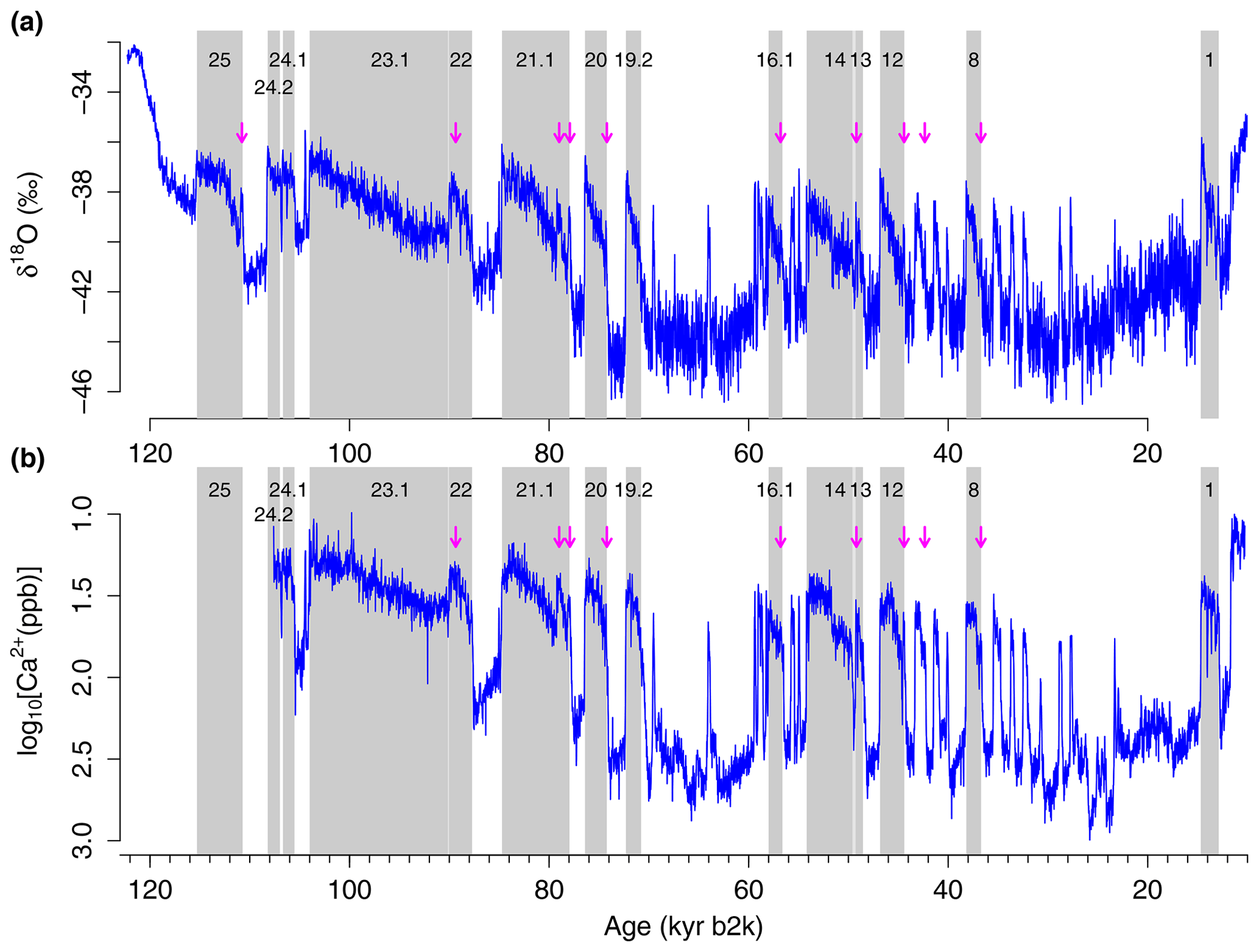
Figure 1 Greenland records from the NGRIP ice core: (a) δ¹⁸O and (b) log ₁₀[Ca²⁺] (Seierstad et al., 2014; Rasmussen et al., 2014). The interstadial parts longer than 1000 years are highlighted with gray shades; their numbering is given at the top of each record (Rasmussen et al., 2014). The rebound events are indicated by arrows (see Sect. 2.1 for their list). Both records are presented at 20-year resolution. The log ₁₀[Ca²⁺] record is available only up to DO-24.1. The compositions of GI-23.1 and GI-22, as well as of GI-14 and GI-13, are considered individual long interstadials (Capron et al., 2010; Rasmussen et al., 2014). The vertical axis for log ₁₀[Ca²⁺] in (b) is reversed to ease visual comparison with the δ¹⁸O record.

Dansgaard–Oeschger (DO) events are millennial-scale abrupt climate transitions during glacial intervals (Dansgaard et al., 1993). They are most clearly imprinted in the δ¹⁸O and calcium ion concentration [Ca²⁺] records from the Greenland ice cores (Fig. 1) (Rasmussen et al., 2014; Seierstad et al., 2014). The δ¹⁸O and [Ca²⁺] are interpreted as proxies for site temperature and atmospheric circulation changes, respectively. DO warmings occur typically within a few decades and are followed by gradual cooling during relatively warm glacial states termed “interstadials”, before a rapid return to cold states referred to as “stadials”. The amplitude of the abrupt warming transitions ranges from 5 to 16.5 °C (Kindler et al., 2014, and references therein). The Greenland temperatures change concurrently with the North Atlantic temperatures (Bond et al., 1993; Martrat et al., 2004), atmospheric circulation patterns (Yiou et al., 1997), seawater salinity (Dokken et al., 2013), sea-ice cover (Sadatzki et al., 2019), and the Atlantic Meridional Overturning Circulation (AMOC), as inferred from indices such as $\mathrm{Pa}/\mathrm{Th}$ and δ¹³C (Henry et al., 2016). The combined proxy evidence suggests that the DO events arise from interactions among these components (Menviel et al., 2020; Boers et al., 2018). The prevailing view is that the mode switching of the AMOC plays a principal role in generating DO events (Broecker et al., 1985; Rahmstorf, 2002), but it remains debated whether the inferred AMOC changes are a driver of DO events or a response to the changes in the atmosphere–ocean–sea-ice system in the North Atlantic, Nordic Seas, and the Arctic (Li and Born, 2019; Dokken et al., 2013). Recently, an increasing number of comprehensive climate models succeeded in simulating DO-like self-sustained oscillations, suggesting that DO events can arise spontaneously from complex interactions between the AMOC, ocean stratification/convection, atmosphere, and sea ice (Peltier and Vettoretti, 2014; Vettoretti et al., 2022; Brown and Galbraith, 2016; Klockmann et al., 2020; Zhang et al., 2021; Kuniyoshi et al., 2022; Malmierca-Vallet and Sime, 2023).

The DO events are considered the archetype of climate tipping behavior (Boers et al., 2022; Brovkin et al., 2021). Early works found an SPS based on autocorrelation for one specific DO warming – the onset of Bølling–Allerød interstadial (Dakos et al., 2008). In subsequent works, the existence of SPS for DO warmings was questioned considering that DO warmings are noise induced rather than bifurcation induced (Ditlevsen and Johnsen, 2010; Lenton et al., 2012). However, a couple of later studies detected SPS for several DO warmings either by ensemble averaging of CSD indicators for many events (Cimatoribus et al., 2013) or by using wavelet-transform techniques focusing on a specific frequency band (Rypdal, 2016; Boers, 2018). On the other hand, it has so far not been shown whether DO coolings are preceded by characteristic CSD-based precursor signals as well.

Recent studies have inferred that the AMOC is currently at its weakest in at least a millennium (Rahmstorf et al., 2015; Caesar et al., 2018) (see also Kilbourne et al. (2022) for possible uncertainties). The declining AMOC trend is projected to continue in the coming century, although the projections of the AMOC strength in the next 100 years are model dependent (Masson-Delmotte et al., 2021). Furthermore, the studies applying CSD indicators to observed AMOC fingerprints (Boers, 2021; Ben-Yami et al., 2023; Ditlevsen and Ditlevsen, 2023) as well as a long-term reconstruction of the Atlantic multidecadal variability (Michel et al., 2022) suggest that the AMOC stability may have declined and the AMOC might be approaching a dangerous tipping point. In this context, it is important to investigate whether CSD-based precursor signals can be detected for the DO cooling transitions as well, supposing that the DO events reflect past AMOC changes. However, of course, predictability of past events does not necessarily imply any predictability in the future, especially given that the recent AMOC weakening is presumably driven by global warming and is thus from a mechanistic point of view different from past AMOC weakenings in the glacial period.

In this study we report SPS for DO cooling transitions recorded in δ¹⁸O and log ₁₀[Ca²⁺] (Seierstad et al., 2014; Rasmussen et al., 2014) from three Greenland ice cores: the North Greenland Ice Core Project (NGRIP), the Greenland Ice Core Project (GRIP), and the Greenland Ice Sheet Project 2 (GISP2) (see Fig. 1 for NGRIP). The important source of observed SPS stems from so-called rebound events, humps in the temperature proxy occurring at the end of interstadials, some decades to centuries prior to the transition (Capron et al., 2010). When CSD indicators such as variance or lag-1 autocorrelation are used for anticipating a tipping point, we conventionally assume that a system gradually approaches a bifurcation point. However, if DO cycles are spontaneous oscillations as suggested in the comprehensive climate models (see above), in a strict sense there might not be any bifurcation occurring around the timings of the abrupt transition in the DO cycles. Nevertheless, with conceptual models of DO cycles, we demonstrate that CSD indicators may show precursor signals for abrupt transitions due to particular dynamics near a critical point or a critical manifold.

The remainder of this paper is organized as follows. In Sect. 2, the data and method are described. In Sect. 3, we identify robust and statistically significant SPSs for several DO cooling transitions following interstadials with sufficient data length and show that rebound events prior to cooling transition are the source of observed SPSs. In Sect. 4 we discuss the results by using conceptual models. A summary is given in Sect. 5.

2 Data and methods

2.1 Greenland ice core records

We explore CSD-based precursor signals for DO cooling transitions recorded in δ¹⁸O and log ₁₀[Ca²⁺] (Seierstad et al., 2014; Rasmussen et al., 2014) from three Greenland ice cores: NGRIP, GRIP, and GISP2 (see Fig. 1 for NGRIP). Multiple records are used for a robust assessment because each has regional fluctuations as well as proxy- and ice-core-dependent uncertainties. The six records have been synchronized and are given at 20-year resolution (Seierstad et al., 2014; Rasmussen et al., 2014). They continuously span the last 104 kyr b2k (kiloyears before 2000 CE), beyond which only NGRIP δ¹⁸O is available up to a part of the Eemian Interglacial. In addition, we use a version of the NGRIP δ¹⁸O and dust records at 5 cm depth resolution (EPICA community members, 2004; Gkinis et al., 2014; Ruth et al., 2003) in order to check the dependence of results on temporal resolutions, with the caveat that these high-resolution records span only the last 60 kyr.

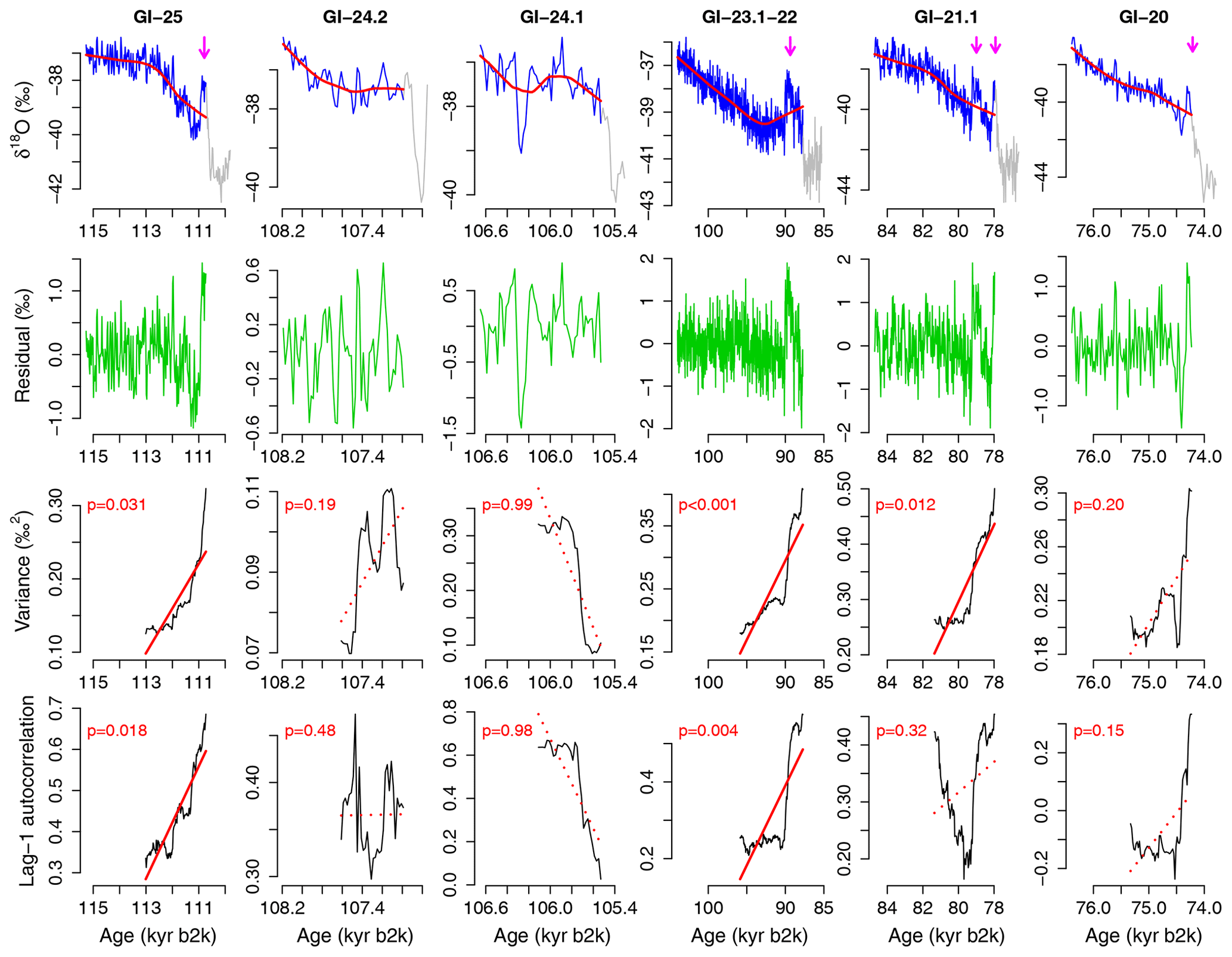
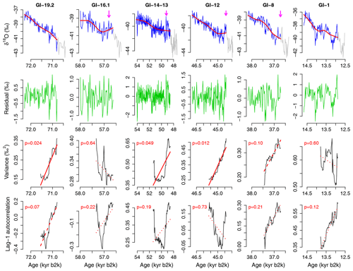
Figure 2 Analysis of CSD-based precursor signals of abrupt DO cooling transitions, for the first six interstadials of NGRIP δ¹⁸O, from 115 ka to 74 kyr b2k. Top row: interstadials longer than 1000 years (blue). The cooling transition and stadial parts are shown in gray (Rasmussen et al., 2014). Nonlinear trends are calculated with the locally weighted scatterplot smoothing (LOESS) (red). The smoothing span α that defines the fraction of data points involved in the local regression is set to 50 % of each interstadial length. The rebound events are indicated by arrows (see Sect. 2.1). Second row: residuals (green) resulting from subtracting the nonlinear trends (red) from the records (blue). Third row: variance estimate in rolling windows (black) with size equal to 50 % of each interstadial length. Values are plotted at the right edge of each rolling window. The linear trend is shown by a solid red line for p<0.05, by a dashed red line for $\mathrm{0.05}<p<\mathrm{0.1}$, and by a dotted line for p>0.1. Fourth row: same as third row but for the lag-1 autocorrelation (i.e., a lag of 20 years).

Figure 3 Same as Fig. 2 but for the next six interstadials, from 74 ka to 12 kyr b2k.

We follow the classification of interstadials and stadials and associated timings of DO warming and cooling transitions by Rasmussen et al. (2014), where Greenland interstadials (stadials) are labeled with “GI” (“GS”) with a few exceptions below. A rebound event is an abrupt warming often observed before an interstadial abruptly ends (Capron et al., 2010) (arrows in Figs. 1, 2, and 3). Generally, a long interstadial accompanies a long rebound event (their durations are correlated with R²=0.95, Capron et al., 2010). In Capron et al. (2010) and Rasmussen et al. (2014), GI-14 and the subsequent interstadial, GI-13, are seen as one long interstadial, with GI-13 considered to be a strongly expressed rebound event ending GI-14 because the changes in δ¹⁸O and log ₁₀[Ca²⁺] during the quasi-stadial GS-14 do not reach the baseline levels of adjacent stadials. Similarly GI-23.1 and GI-22 are also seen as one long interstadial, and GI-22 is regarded as a rebound event (and GS-23.1 as quasi-stadial) (Capron et al., 2010; Rasmussen et al., 2014). GI-20a is also recognized as a rebound event in Rasmussen et al. (2014). Given that the rebound events are warmings following a colder spell during interstadial conditions that does not reach the stadial levels (Rasmussen et al., 2014), we regard the following nine epochs as rebound-type events: GI-8a, the hump at the end of GI-11 (42 240–∼42 500 yr b2k), GI-12a, GI-13, the hump at the end of GI-16.1 (56 500–∼56 900 yr b2k), GI-20a, GI-21.1c-b-a (two warming transitions), GI-22, and GI-25a. When we examine the effect of rebound events on our results, we exclude the entire parts including the cold spells prior to the rebound events.

The start (warming) and end (cooling) of each DO event are identified in 20-year resolution based on both δ¹⁸O and [Ca²⁺] in Rasmussen et al. (2014). The estimated uncertainty of event timing varies from event to event. We remove the 2σ uncertainty range of the event timing (40 to 400 years) estimated in Rasmussen et al. (2014) from our calculation of CSD indicators. It effectively excludes parts of the transitions themselves from the calculation of the CSD indicators. Since the calculation of CSD indicators requires a minimum length of data points, we mainly focus on interstadials longer than 1000 years after removing 2σ uncertainty ranges of the transition timings, using 20-year resolution data (Table S1 in the Supplement). This results in 12 DO interstadials to be investigated (Fig. 1, gray shades). We deal with the interstadials shorter than 1000 years but longer than 300 years using high-resolution records in Sect. 3.2.

2.2 Statistical indicators of critical slowing down

Based on the theory of critical slowing down (CSD), we posit that the stability of a dynamical system perturbed by noise is gradually lost as the system approaches a bifurcation point (Boers et al., 2022; Scheffer et al., 2009; Bury et al., 2020). For the fold bifurcation (also known as the saddle-node bifurcation), the variance of the fluctuations around a local stable state diverges and the autocorrelation function of the fluctuations increases toward 1 at any lag τ. The same is true for the transcritical as well as the pitchfork bifurcation (Bury et al., 2020). For the Hopf bifurcation, the variance increases, but the autocorrelation function of the form $C\left(\mathit{\tau }\right)=e^{\mathit{\nu }\left|\mathit{\tau }\right|}\cos \mathit{\omega }\mathit{\tau }$ may increase or decrease depending on τ, where ν(≤0) and ±ωi are the real and imaginary parts of the complex eigenvalues of the Jacobian matrix of the local linearized system (Bury et al., 2020). Nevertheless, the autocorrelation function C(τ) increases for sufficiently small τ. For discrete time series, we follow previous studies and calculate the lag-1 autocorrelation corresponding to a minimal τ. These characteristics can be used to anticipate abrupt transitions caused by codimension-1 bifurcations. Promisingly previous studies show that these CSD indicators and related measures can indeed anticipate simulated AMOC collapses (Boulton et al., 2014; Klus et al., 2018; Livina and Lenton, 2007; Held and Kleinen, 2004).

Prior to calculating CSD indicators, we estimate the local stable state by using a local regression method called the locally weighted scatterplot smoothing (LOESS) (Cleveland et al., 1992; Dakos et al., 2012). In this approach, the time series is seen as a scatter plot and fitted locally by a polynomial function, giving more weight to points near the point whose response is being estimated and less weight to points further away. Here the polynomial degree is set to 1; i.e., the smoothing is performed with the local linear fit. Nevertheless, the LOESS provides nonlinear smoothed curves. The smoothing span parameter α that defines the fraction of data points involved in the local regression is set to 50 % of each interstadial length in a demonstration case, but we examine the dependence of results on α over the range 20 %–70 %. The difference between the record and the smoothed one gives the residual fluctuations. The CSD indicators, i.e., variance and lag-1 autocorrelation, are calculated for the residuals over a rolling window. The size W of this rolling window is set to 50 % of each interstadial length in the demonstration case. To test the robustness, this is changed over the range 20 %–60 %.

The statistical significance of precursor signals of critical transitions, in terms of positive trends of CSD indicators, is assessed by hypothesis testing (Theiler et al., 1992; Dakos et al., 2012; Rypdal, 2016; Boers, 2018). We consider as null model a stationary stochastic process with preserved variance and autocorrelation. The n surrogate data are prepared from the original residual series by the phase-randomization method, thus preserving the variance and autocorrelation function of the original time series via the Wiener–Khinchin theorem. Here we take n=1000. The linear trend (a_o) of the CSD indicator for the original time series and the linear trends (a_s) of CSD indicators for the surrogate data are calculated. We consider the precursor signal of the original time series statistically significant at the 5 % level if the probability of a_s>a_o (p value) is less than 0.05. The significance level of 0.05 is conservative given that some works analyzing ecological or paleo-data adopt the significance level of 0.1 (Dakos et al., 2012; Thomas et al., 2015).

3 Results

3.1 Characteristic precursor signals of DO coolings

As CSD indicators we consider the variance and lag-1 autocorrelation, calculated in rolling windows across each interstadial. The 12 interstadials longer than 1000 years are magnified in Figs. 2 and 3 (top rows, blue) for the NGRIP δ¹⁸O record. See Figs. S1–S10 in the Supplement for the other records. For each interstadial, the nonlinear trend is estimated using LOESS smoothing (Figs. 2 and 3, top row, red). In this case the smoothing span α that defines the fraction of data points involved in the local regression is set to 50 % of each interstadial length. Gaussian kernel smoothing gives similar results. The difference between the record and the nonlinear trend gives the approximately stationary residual fluctuations (second row). The CSD indicators are calculated from the residual series over a rolling window. In Figs. 2 and 3 the rolling window size W is set to 50 % of each interstadial length (a default value in Dakos et al., 2008). The smoothing span α and the rolling window size W are taken as fractions of individual interstadial length because timescales of local fluctuations (such as the duration of rebound events) change with the entire duration of interstadial. We examine the dependence of the results on α and W as part of our robustness tests.

The variance is plotted in the third row of Figs. 2 and 3. Positive trends in the variance are observed for 9 out of 12 interstadials; the individual trends are statistically significant in 6 out of 12 cases (p<0.05), based on a null model assuming the same overall variance and autocorrelation, constructed by producing surrogates with randomized Fourier phases. The lag-1 autocorrelation is also plotted for the same data in the bottom row. Positive trends in lag-1 autocorrelation are observed for 10 out of 12 interstadials but are statistically significant only in two cases (p<0.05). Just a positive trend without significance cannot be considered a reliable SPS, but if one indicator has a significantly positive trend, the other indicator with a consistently positive trend may at least support the conclusion (e.g., GI-19.2 and GI-14-13 in Fig. 3). In several cases (GI-24.2, GI-21.1, GI-16.1, GI-14-13, and GI-12), the lag-1 autocorrelation first decreases and then increases. The initial decreases, harming monotonic increases of CSD indicators, might reflect a memory of the preceding DO warming transition. On the other hand, the drastic increases in both indicators near the end of the interstadials reflect the rebound events (arrows in Figs. 2 and 3). We obtain similar results for the other ice core records (Figs. S1–S10). While we observe a number of positive trends for all the records, the number of statistically significant trends detected depends on the record and CSD indicator (Table S2).

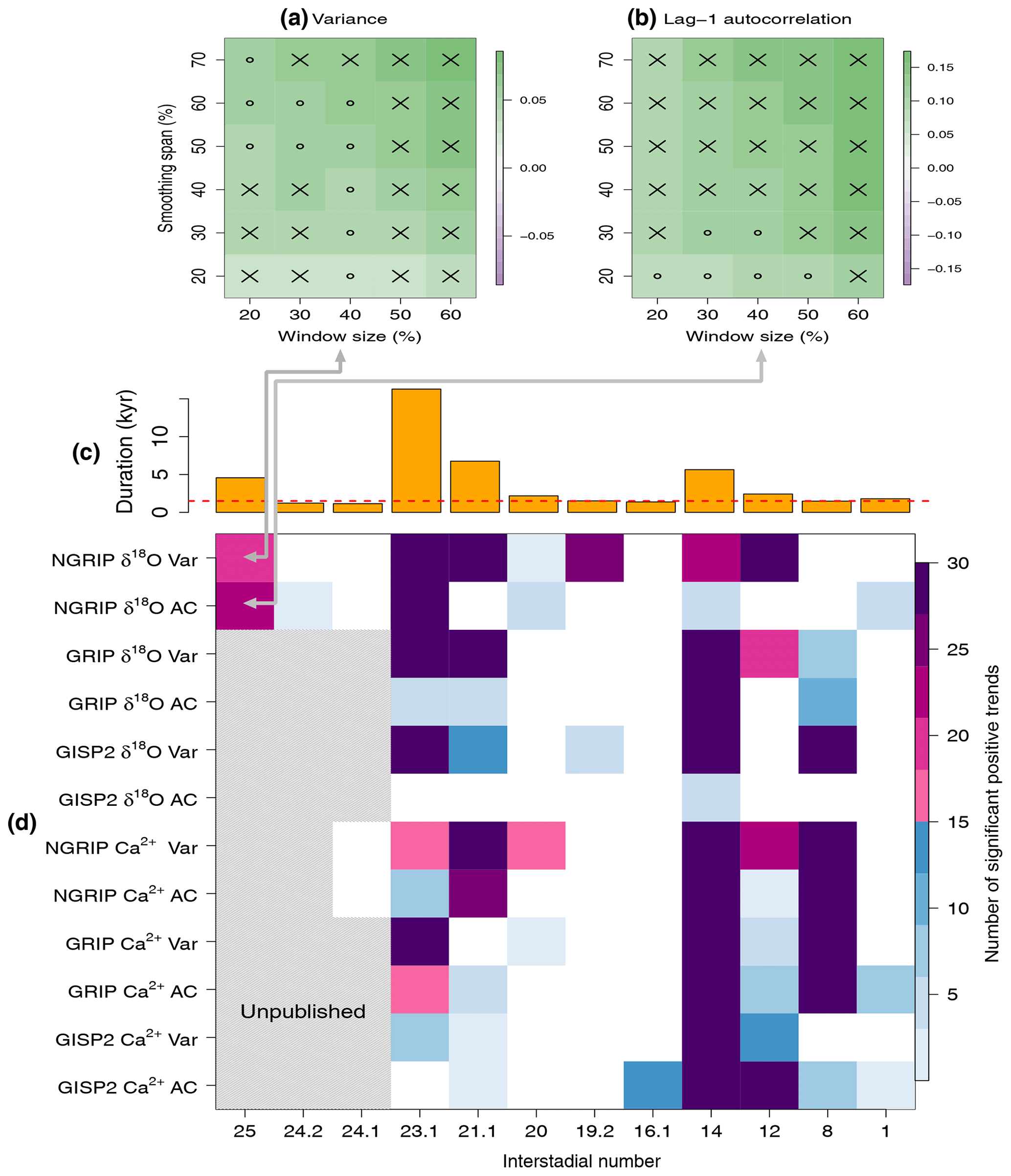
Figure 4 Detection of precursor signals of DO cooling transitions for different interglacials, different proxy variables, different ice cores, and different CSD indicators. (a, b) Robustness analysis of precursor signals with respect to the smoothing span and the rolling window size (% of interstadial length): the case of the GI-25 interstadial from the NGRIP δ¹⁸O record. The CSD indicator is the variance in (a) and the lag-1 autocorrelation in (b). Cross marks (x) indicate statistically significant positive trends of the respective CSD indicator (p<0.05) based on a phase surrogate test (see Sect. 2.2), small open circles (o) indicate barely significant positive trends ($\mathrm{0.05}<p<\mathrm{0.1}$), and cells are left blank if p>0.1. (c) Durations of interstadials longer than 1000 years (Table S1). The dashed line indicates 1500 years (d). Robustness of finding precursor signals for DO cooling transitions. The color indicates the number of significant (p<0.05) positive trends in each of the 30 sets of the smoothing spans and the rolling window sizes as in (a) and (b). For the cases of gray-shaded cells, the data are not publicly available.

We check the robustness of our results against changing smoothing span α and rolling window size W (Dakos et al., 2012). We calculate the p value for the trend of each indicator changing the smoothing span between 20 % and 70 % of interstadial length (in steps of 10 %) and the rolling window size between 20 % and 60 % (also in 10 % steps). This yields a 6×5 matrix for the p values. Example results for GI-25 and δ¹⁸O are shown in Fig. 4a (variance) and 4b (lag-1 autocorrelation). The cross mark (x) indicates significant positive trends (p<0.05) and the small open circle (o) indicates positive trends that are significant at the 10 % level but not at the 5 % level. Full results for the 12 interstadials, six records, and two CSD indicators are shown in Figs. S11–S22. We consider positive trends in CSD indicators, i.e., the SPS of the transition, to be overall robust if we obtain significant positive trends (p<0.05) for more than half (>15) of the 30 parameter sets.

The robustness analysis is performed for all the long interstadials of the six records and the two CSD indicators (Fig. 4d). Among the 12 interstadials, we find at least one robust SPS for eight interstadials (GI-25, GI-23.1, GI-21.1, GI-20, GI-19.2, GI-14, GI-12, and GI-8) and multiple robust SPSs for six (GI-25, GI-23.1, GI-21.1, GI-14, GI-12, and GI-8). If the data series is a stationary stochastic process, the probability of spuriously observing a robust SPS is estimated to be 5 % (Appendix A). In this case, the probability of detecting more than two robust SPSs from 12 independent stationary samples (i.e., from each row in Fig. 4d) by chance is only ∼2 %. Thus, the risk of obtaining the results by chance is quite low. For each interstadial, the detection of robust SPSs depends on the proxy and core. This is possibly because different proxies from different cores are contaminated by different types and magnitudes of noise (e.g., δ¹⁸O may record local fluctuations of temperatures and log ₁₀[Ca²⁺] turbulent fluctuations of local wind circulations). Robust SPSs are observed for most interstadials longer than roughly 1500 years (GI-25, GI-23.1, GI-21.1, GI-20, GI-19.2, GI-14, GI-12, and GI-8 except GI-1) but not for the other interstadials, shorter than roughly 1500 years (compare Figs. 4c and 4d).

3.2 Further sensitivity analyses

We examine how much the rebound events affect the detection of CSD-based SPS. For this purpose CSD indicators are again calculated excluding the rebound events and their preceding cold spells (see Sect. 2.1). While eight interstadials (GI-25, GI-23.1, GI-21.1, GI-20, GI-16, GI-14, GI-12, and GI-8) exhibit robust SPS with the rebound events included, only four interstadials (GI-23.1, GI-14, GI-12, and GI-8) exhibit robust SPS without the rebound events (Fig. S23). The rebound events should hence be considered important, sometimes indispensable, sources for SPS of DO coolings.

We also examine the dependence of the results on the time resolution of the data. Here we use a high-resolution (5 cm depth) δ¹⁸O record (EPICA community members, 2004; Gkinis et al., 2014) and a dust record (Ruth et al., 2003) from the NGRIP over the last 60 kyr. Since the data in these records are non-uniform in time, they are linearly resampled every 5 years before calculating CSD indicators. We focus on 11 interstadials longer than 300 years in order to have enough data points. For the dust record, three interstadials (GI-15, GI-8, and GI-7) are excluded from the analysis because the original data have long parts of missing values. The CSD indicators, calculated with a smoothing span of α=50 % and rolling windows of W=50 %, are shown in Figs. S24–S27. Through the robustness analyses with respect to α and W, we find at least one robust SPS for three out of 11 interstadials (Fig. S28). The robust SPSs for GI-14-13 and GI-12 from the high-resolution records are consistent with those from the 20-year resolution records. Moreover for GI-1, the high-resolution δ¹⁸O record exhibits a robust SPS in terms of lag-1 autocorrelation, although the 20-year resolution record does not. Robust SPSs have not been observed again for interstadials shorter than roughly 1500 years (Figs. S28 and 4).

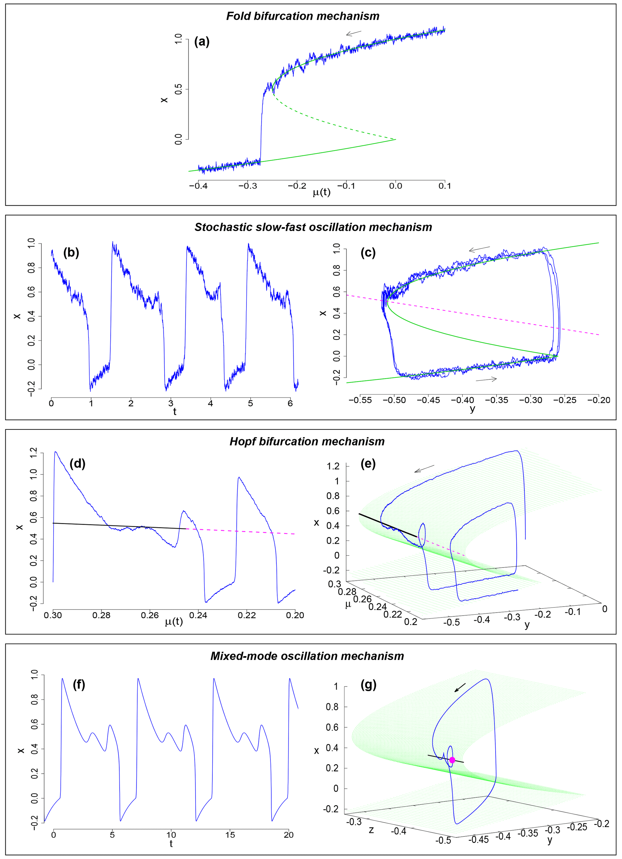
Figure 5 Four potential dynamical mechanisms for the DO cooling transitions. (a) Fold bifurcation mechanism. The time series x(t) for decreasing μ(t) (blue). The green lines show the stable (solid) and unstable (dashed) fixed points. (b, c) Stochastic slow–fast oscillation mechanism of a FitzHugh–Nagumo-type model. An example time series x(t) is shown in (b) and the phase space trajectory (blue) in (c); the x nullcline, i.e., the critical manifold, is shown in green. The y nullcline is shown in dashed magenta. (d, e) Hopf bifurcation mechanism. An example time series x(t) is shown in (d) as a function of μ(t). Stable (black, solid) and unstable (magenta, dashed) fixed points are also shown. The corresponding phase space trajectory (x(t),y(t)) for decreasing μ is shown in (e) in blue. The critical manifold is shown in green. (f, g) Mixed-mode oscillation mechanism. An example time series x(t) is shown in (f) and the corresponding phase space trajectory in (g). The magenta dot is the saddle point with a stable manifold in the direction of the black segment; the trajectory is spiralling around it.

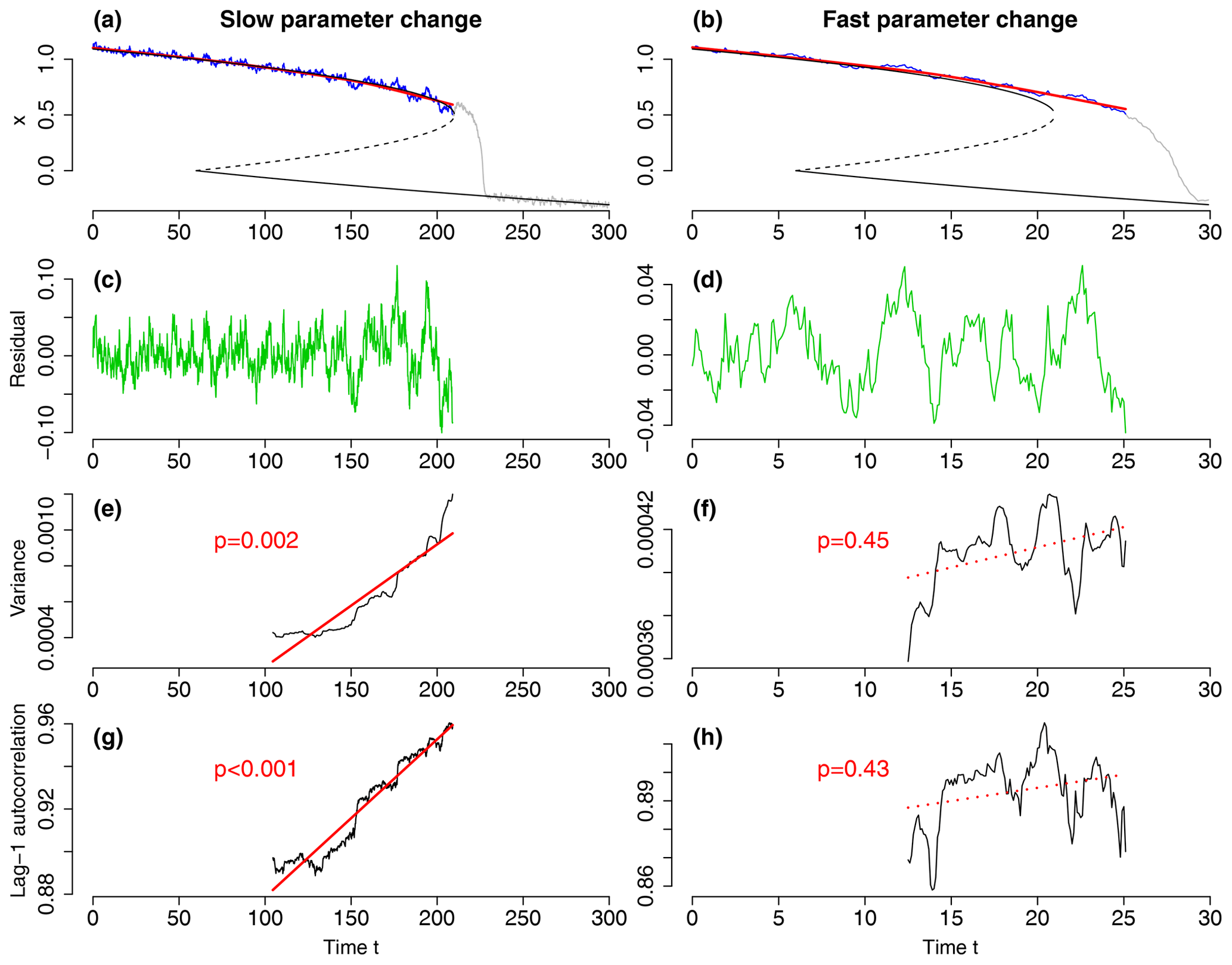
Figure 6 Rate dependence of CSD indicators for the fold bifurcation in the Stommel model. Its parameter μ(t) is decreased from μ=0.1 to $\mathit{\mu }=-\mathrm{0.4}$ across the fold bifurcation point $\mathit{\mu }=-\mathrm{0.25}$ with a small rate $\dot{\mathit{\mu }}\left(t\right)=-\mathrm{1}/\mathrm{600}$ (left column) or with a 10 times larger rate $\dot{\mathit{\mu }}\left(t\right)=-\mathrm{1}/\mathrm{60}$ (right column). (a, b) Dynamical variable x(t) before the tipping (blue) and after the tipping (gray). The time interval of sampling x(t) value is 0.1 in both cases. The solid black lines and the dashed lines show the stable equilibria and the unstable equilibrium, respectively. (c, d) Residuals (green) resulting from subtracting the nonlinear trends (red) from the records (blue). (e, f) Variance estimate in rolling windows (black) with size equal to 50 % of the signal before tipping. Values are plotted at the right edge of each rolling window. The linear trend is shown by a solid red line for p<0.05 and by a dotted line for p>0.1. (g, h) Same as (e, f) but for the lag-1 autocorrelation. Significant increases of CSD indicators are unlikely to be observed when the parameter changes rapidly. Typical cases are shown here. Details of trajectories and the changes of CSD indicators depend on noise realizations.

4 Possible dynamical mechanisms

We detected robust precursor signals of DO cooling transitions for most interstadials longer than roughly 1500 years but not for shorter interstadials. The results suggest that long interstadials, the existence of rebound events, and the presence of SPS for the DO cooling transitions are all related (except for GI-19.2, which has no noticeable rebound event). These aspects may be related to generic properties of nonlinear dynamical systems. On the basis of conceptual mathematical models, we discuss four possible dynamical mechanisms leading to the precursor signals of DO cooling transitions. In three of four mechanisms, oscillations such as the rebound events can systematically arise prior to the abrupt cooling transitions. These modeling results justify the inclusion of the rebound events in the search for precursor signals presented above. Unless otherwise mentioned, details on model parameters as well as the hysteresis experiments conducted are given in Appendix B.

1. The fold bifurcation mechanism. Since the pioneering work by Stommel (1961), the AMOC is considered to exhibit bistability depending on the background condition (Rahmstorf, 2002). The bistability of the AMOC strength x may be conceptually modeled by a double-fold bifurcation model: $\dot{x}=f\left(x\right)+\mathit{\mu }+\mathit{\xi }\left(t\right)$, where f(x) has two fold points such as x−x³ and $\left|x\right|(\mathrm{1}-x)$. Here we take the quadratic from $f\left(x\right)=\left|x\right|(\mathrm{1}-x)$, but the following arguments are qualitatively the same for x−x³. The parameter μ represents the surface salinity flux (i.e., negative freshwater flux), and ξ(t) denotes white Gaussian noise. The unperturbed model for ξ(t)=0 has equilibria on an S-shaped curve: $f\left(x\right)+\mathit{\mu }=\mathrm{0}$ (Fig. 5a, green). The state x(t) initially on the upper stable branch jumps down to the lower stable branch as μ decreases across the fold bifurcation point at $\mathit{\mu }=-\mathrm{0.25}$. The variance and the autocorrelation of the local fluctuations (i.e., CSD indicators) increase as μ slowly approaches the fold bifurcation point since the restoring rate toward the stable state decreases, as shown in Fig. 6a (Scheffer et al., 2009; Boers et al., 2022).

2. Stochastic slow–fast oscillation mechanism. The FitzHugh–Nagumo (FHN) system is a prototypical model for slow–fast oscillations and excitability (FitzHugh, 1961; Nagumo et al., 1962). It is often invoked for conceptual models of DO oscillations (Rial and Yang, 2007; Kwasniok, 2013; Roberts and Saha, 2017; Mitsui and Crucifix, 2017; Lohmann and Ditlevsen, 2019; Riechers et al., 2022; Vettoretti et al., 2022). An FHN-type model of DO oscillations can be obtained by introducing a slow variable y into the fold bifurcation model: $\dot{x}=\frac{\mathrm{1}}{{\mathit{\tau }}_x}\left(\right|x\left|\right(\mathrm{1}-x)+y+\mathit{\mu })+\mathit{\xi }\left(t\right)$, $\dot{y}=\frac{\mathrm{1}}{{\mathit{\tau }}_y}(-x-y)$, where τ_x and τ_y are timescale parameters (τ_x≪τ_y). Invoking the salt-oscillator hypothesis for DO oscillations suggested by the comprehensive climate model simulations that are successful in reproducing DO cycles (Vettoretti and Peltier, 2018), we may interpret y as the surface mixed-layer salinity in the northern North Atlantic and Labrador Sea, which gradually decreases (increases) when the AMOC intensity x is strong (weak).

   Here we consider the case that the system is excitable. For example, for μ=0.26, the unperturbed system has a stable equilibrium near the upper fold point of the S-shaped critical manifold, $\mathit{\left\{}\right(x,y)\in {\mathbb{R}}^{\mathrm{2}}|y=-\left|x\right|(\mathrm{1}-x)-\mathit{\mu }\mathit{\}}$ (Fig. 5c, green), but the dynamical noise ξ(t) enables the escape from the barely stable equilibrium and sustains stochastic oscillations (Fig. 5b and c, blue). Due to the timescale separation (τ_x≪τ_y), the oscillations occur along the attracting parts of the critical manifold (Fig. 5c). Because y is much slower than x, the dynamics of x is similar to the dynamics of the fold bifurcation model with slowly changing y. As a result, SPS can be effectively observed near the upper fold point of the critical manifold (Fig. S29). However, this example is not rigorous bifurcation-induced tipping. In the example of an excitable system (Fig. 5b and c), the underlying system always has a weakly stable fixed point, and no true bifurcation leading to CSD occurs. In fact, the actual tipping in this case is noise induced. However, we can effectively observe the SPS in CSD indicators in this case as well, since the system would in each cyclic iteration move from more stable to less stable conditions until it finally tips to initiate the next cycle, and this partial decrease in stability is imprinted in the CSD indicators (Fig. S29). The increase of the variance prior to the transitions in the FHN model is also reported in Meisel and Kuehn (2012). Since the unperturbed system has an equilibrium near the upper fold point, the motion is stagnant near the fold point. This provides favorable conditions for observing SPS. The state jumps from the upper branch of the critical manifold to its lower branch often occur after an upward jump induced by noise. These upward jumps resemble the rebound events prior to DO cooling transitions. The overall phenomenon is the same in the self-sustained oscillation regime of the FHN model, as long as the equilibrium is located near the upper fold point of the critical manifold (μ≃0.25).

3. Hopf bifurcation mechanism. In contrast to the fold bifurcation, the Hopf bifurcation manifests oscillatory instability (Strogatz, 2018). In several ocean box models, the thermohaline circulation is destabilized via a Hopf bifurcation (Alkhayuon et al., 2019; Lucarini and Stone, 2005; Abshagen and Timmermann, 2004; Sakai and Peltier, 1999). It is also considered a potential generating mechanism of DO oscillations in a low-order coupled climate model (Timmermann et al., 2003) and in a comprehensive climate model (Peltier and Vettoretti, 2014). Assume that the parameter μ decreases slowly in the FHN-type model (Fig. 5d and e). The underlying dynamics changes from the stable equilibrium to the limit-cycle oscillations at the Hopf bifurcation point $\mathit{\mu }={\mathit{\mu }}_{\text{Hopf}}\equiv (\mathrm{1}-{\mathit{\tau }}_x/{\mathit{\tau }}_y{)}^{\mathrm{2}}/\mathrm{4}$ (Appendix B). If stochastic forcing is added to the system, noise-induced small oscillations can appear prior to the onset of the limit-cycle oscillations (Fig. 5d and e). The precursor oscillations resemble rebound events, while their shape depends on the noise as well as the change rate of μ. Again SPS can be observed near the Hopf bifurcation point (Fig. S30) (Bury et al., 2020; Meisel and Kuehn, 2012; Boers et al., 2022). The small oscillations prior to downward transitions, like the DO rebound events, do not appear if the system goes deeply into the self-sustained oscillation regime away from the Hopf bifurcation point ($\mathit{\mu }<{\mathit{\mu }}_{\text{Hopf}}\approx \mathrm{0.245}$ in Fig. 5d).

4. Mixed-mode oscillation mechanism. Mixed-mode oscillations (MMOs) are periodic oscillations consisting of small- and large-amplitude oscillations (Koper, 1995; Desroches et al., 2012; Berglund and Landon, 2012). They often arise in systems with one fast variable and two slow variables (Desroches et al., 2012). In this regard, we can extend the above FHN-type model to exhibit MMOs, for example, as follows: $\dot{x}=\frac{\mathrm{1}}{{\mathit{\tau }}_x}\left(\right|x\left|\right(\mathrm{1}-x)+y+\mathit{\mu })$, $\dot{y}=\frac{\mathrm{1}}{{\mathit{\tau }}_y}(-x-y+k(z-y\left)\right)$ and $\dot{z}=\frac{\mathrm{1}}{{\mathit{\tau }}_z}(-x-z+k(y-z\left)\right)$, where z is another slow variable with timescale τ_z (≫τ_x) and k is the diffusive-coupling constant between slow variables. We interpret y as the surface salinity in the northern North Atlantic convection region that directly affects the AMOC strength x again and z as the surface salinity outside the convection region that affects the surface salinity y in the convection region via mixing. This extended FHN-type model is introduced here only to demonstrate that MMOs may appear in an FHN-type model with a minimal dimensional extension. For certain parameter settings (Appendix B), the system has an unstable equilibrium $(x,y,z)=(\sqrt{\mathit{\mu }},-\sqrt{\mathit{\mu }},-\sqrt{\mathit{\mu }})$ of saddle-focus type, with one stable direction with a negative real eigenvalue and a two-dimensional unstable manifold with complex eigenvalues with a positive real part. The slow–fast oscillations occur along the critical manifold $\mathit{\left\{}\right(x,y,z)\in {\mathbb{R}}^{\mathrm{3}}|y=-\left|x\right|(\mathrm{1}-x)-\mathit{\mu }\mathit{\}}$ (Fig. 5f and g). However, due to the saddle-focus equilibrium on the critical manifold, the trajectory is attracted toward the saddle from the direction of the stable manifold (black segment) and repelled from it in a spiralling fashion. The striking point is the systematic occurrence of small-amplitude oscillations prior to the abrupt transition, which also resemble the rebound events prior to the DO cooling transitions. A more realistic time series is obtained if an observation noise is added on x(t) (Fig. S31). Then SPS can be stably observed near the fold point of the critical manifold.

Based on the four types of simple mathematical models, we have proposed four possible dynamical mechanisms for the DO cooling transitions that can manifest statistical precursor signals (SPS): (1) strict CSD due to the approaching of a fold bifurcation; (2) CSD in a wider sense, in stochastic slow–fast oscillations; (3) noise-induced oscillations prior to Hopf bifurcations; or (4) the signal of mixed-mode oscillations. While the details of these mechanisms are different, they are all related to the fold points of the equilibrium curve or the critical manifolds. As a result, the SPS can be detected by the conventional CSD indicators.

Mechanisms (2), (3), and (4) can generate behavior resembling the rebound events, leading to increases in the classic CSD indicators. In the toy models, rebound event-like behavior is generated when the trajectory passes by an equilibrium point with marginal stability (i.e., the equilibrium has neither strong stability leading to a permanent state nor strong instability leading to short interstadials) (Fig. 5b–g). In this case, the duration of the modeled interstadial is relatively long in relation to the marginal stability. By contrast, the absence of equilibrium or the presence of a strongly unstable equilibrium near the fold point of the critical manifold leads to brief interstadials without a rebound event and consequently a lack of SPS. This provides a possible explanation of why the rebound events and the robust SPS are simultaneously observed for long interstadials but not for short interstadials.

Another possible explanation for the lack of SPS for short interstadials is the following. The common assumption underlying CSD theory is that the parameter change is much slower than the system's relaxation time, and the latter is much slower than the correlation time of the noise (Thompson and Sieber, 2011; Ashwin et al., 2012). If this assumption is violated, it is difficult to detect CSD-based SPS (Clements and Ozgul, 2016; van der Bolt et al., 2021). Consider the fold-bifurcation-induced tipping in the Stommel-type model (1), for example (Fig. 6). If the change in the parameter μ is faster than the system's relaxation time toward the moving stable equilibrium, it is unlikely to detect significant CSD-based SPS (Fig. 6b) because the trajectory evolves systematically away from the equilibrium and thus cannot feel the flattening of the potential around the equilibrium even at the true bifurcation point.

5 Summary and discussion

In this study we have explored statistical precursor signals (SPSs) and significant increases in critical slowing down (CSD) indicators (variance and lag-1 autocorrelation), for Dansgaard–Oeschger (DO) cooling transitions following interstadials, using six Greenland ice core records. Among the 12 interstadials longer than 1000 years, we find at least one robust SPS for eight interstadials longer than roughly 1500 years (GI-25, GI-23.1, GI-21.1, GI-20, GI-19.2, GI-14, GI-12, and GI-8) and multiple robust SPSs for six of them (GI-25, GI-23.1, GI-21.1, GI-14, GI-12, and GI-8) (Fig. 4d). Robust SPSs are, however, not observed for interstadials shorter than roughly 1500 years. One might link the increase in the proxy variance with the tendency of larger climatic fluctuations in colder climates (Ditlevsen et al., 1996), but the increases in the lag-1 autocorrelation cannot generally be explained by it. The analysis removing the rebound events from the data shows that the rebound events prior to the cooling transitions are important in producing the SPS.

We have proposed four different dynamical mechanisms to explain the observed SPSs: (1) strict CSD due to the approaching of a fold bifurcation; (2) CSD in a wider sense, in stochastic slow–fast oscillations; (3) noise-induced oscillations prior to Hopf bifurcations; or (4) the signal of mixed-mode oscillations. In the last three mechanisms, oscillations such as the rebound events can systematically arise prior to the abrupt cooling transitions. These precursor oscillations are due to marginally (un)stable equilibria on the critical manifolds that cause a long-lived quasi-stable state (like long interstadials). This can explain why rebound events and SPSs are simultaneously observed only for long interstadials and are not observed for short ones. While the SPSs for bifurcation-induced tipping events (mechanisms 1 and 3) are established, detailed properties of SPSs for the stochastic slow–fast oscillations of the excitable system (mechanism 2) and for the mixed-mode oscillations (mechanism 4) remain to be elucidated.

We should mention the assumptions made in this study as well as alternative scenarios for the DO cooling transitions. First, the four dynamical mechanisms assume slow changes in parameters or slow variables which cause bifurcations in the fast subsystem. On the other hand, the rate-induced tipping mechanism has also been invoked for a possible AMOC collapse, where the rate of change of the external forcing (e.g., freshwater flux or atmospheric CO₂ concentration) determines the future AMOC state (Alkhayuon et al., 2019; Lohmann and Ditlevsen, 2021; Ritchie et al., 2023). The lack of observed SPSs for the interstadials less than roughly 1500 years indicates a rate-dependent aspect of the DO cooling transitions. However, a comprehensive investigation of DO cooling transitions from the viewpoint of rate-induced tipping is beyond the scope of this work. Second, a recent study using an ocean general circulation model shows that a rebound-event-type behavior of AMOC is caused by a behavior called “the intermediate tipping”, due to multiple stable ocean circulation states that exist near but prior to the tipping point leading to a significant AMOC weakening (Lohmann et al., 2023). The intermediate tipping mechanism for rebound events is different from the possible low-dimensional dynamical mechanisms proposed in this study. Further studies are needed to elucidate the dynamical as well as physical origin of DO coolings and associated rebound events.

We have shown that past abrupt DO cooling transitions in the North Atlantic region can be anticipated based on classic CSD indicators if they are preceded by long interstadials. However, it is found to be difficult to anticipate DO cooling events, at least from the 20-year-resolution ice core Greenland records, if they occur after a short interstadial. If the DO coolings transitions are actually associated with AMOC weakening (see the “Introduction”), our results may have an implication for the predicted weakening of the AMOC and its possible collapse in the future: the prediction with CSD indicators could be more difficult if the forcing changes fast. There is, however, a caveat to this implication because the past DO cooling transitions are different from the presently inferred AMOC changes. The time resolution (mainly 20 years and additionally 5 years) and the length (mainly >1000 years and additionally >300 years) of the interstadial segment data used in this study are coarser and mostly longer than the annual data used for analyzing AMOC fingerprints during the industrial period (Boers, 2021; Ben-Yami et al., 2023; Ditlevsen and Ditlevsen, 2023) and the last millennium (Michel et al., 2022). More crucially, the revealed predictability of past DO cooling events does not necessarily imply predictability of a potential future AMOC collapse since the recent AMOC weakening, possibly driven by global warming but potentially also part of natural variability, is mechanistically very different from past AMOC weakening in the glacial period.

Appendix A: Probability of observing robust precursor signals

The statistical significance of precursor signals of critical transitions, in terms of positive trends of CSD indicators, is assessed by hypothesis testing (Theiler et al., 1992; Dakos et al., 2012; Rypdal, 2016; Boers, 2018). We consider a stationary stochastic process with preserved variance and autocorrelation as the null model. The n surrogate data are prepared from the original residual data series by the phase-randomization method, thus preserving the variance and autocorrelation function of the original time series via the Wiener–Khinchin theorem. Here we take n=1000. The linear trend (a₀) of the CSD indicator for the original residual time series and the linear trends (a_s) of CSD indicators for the surrogate data are calculated. We consider the precursor signal of the original series statistically significant at the 5 % level if the probability of a_s>a_o (p value) is less than 0.05. Thus, if the original data are already a stationary stochastic process (exhibiting no CSD), one should expect spuriously significant results at a probability of 0.05 by definition. In principle this is independent of the smoothing span α as well as the rolling window size W used for calculating CSD indicators. We consider a precursor signal robust if we find significant cases (p<0.05) for more than half (>15) of 30 combinations of α and W. Then the probability of observing a robust precursor signal can be shown to be 0.05. In order to check this numerically, we generate 5000 surrogates of the original δ¹⁸O series of interstadial GI-25 and calculate the probability of finding robust precursor signals. The resulting fractions are 0.041 for the variance and 0.039 for the lag-1 autocorrelation, which are close to 0.05. For the case of GI-12, we obtain 0.038 for the variance and 0.047 for the lag-1 autocorrelation, again close to 0.05. These results support the probability of observing a robust precursor signal being 5 % if the data are stationary stochastic processes.

Appendix B: Details of conceptual models used in Fig. 5

Here we describe specific settings for four conceptual models representing different candidate mechanisms for the DO cooling transitions. Unless otherwise mentioned, the stochastic differential equations below are solved with the Euler–Maruyama method with a step size of 10⁻³.

1. The bistability of the AMOC strength x can be conceptually modeled by a double-fold bifurcation model: $\dot{x}=f\left(x\right)+\mathit{\mu }+\mathit{\xi }\left(t\right)$, where f(x) has two fold points; here for f one can use either $f\left(x\right)=x-x^{\mathrm{3}}$ or $f\left(x\right)=\left|x\right|(\mathrm{1}-x)$. We take the quadratic function $f\left(x\right)=\left|x\right|(\mathrm{1}-x)$ that arises in the Stommel (1961) model. μ represents a forcing parameter on the AMOC strength x, e.g., salinity forcing on the North Atlantic (i.e., negative freshwater forcing). ξ(t) is white Gaussian noise, e.g., freshwater perturbations or weather forcing. In Fig. 5a, we set $\sqrt{\langle {\mathit{\xi }}^{\mathrm{2}}\rangle }=\mathrm{0.03}$, and the initial condition is taken at x(0)=1.1, near the upper stable fixed point of the unperturbed system. The parameter μ is then slowly decreased from 0.1 to −0.4 over the period from t=0 to t=500, to trigger the bifurcation-induced transition.

2. The FitzHugh–Nagumo-type (FHN-type) system is a prototypical model of slow–fast oscillators (FitzHugh, 1961; Nagumo et al., 1962) and often invoked for conceptual models of DO oscillations (Rial and Yang, 2007; Kwasniok, 2013; Roberts and Saha, 2017; Mitsui and Crucifix, 2017; Lohmann and Ditlevsen, 2019; Riechers et al., 2022; Vettoretti et al., 2022). The FHN-type model subjected to dynamical noise can be obtained by introducing a slow variable y into the fold bifurcation model: $\dot{x}=\frac{\mathrm{1}}{{\mathit{\tau }}_x}\left(\right|x\left|\right(\mathrm{1}-x)+y+\mathit{\mu })+\mathit{\xi }\left(t\right)$, $\dot{y}=\frac{\mathrm{1}}{{\mathit{\tau }}_y}(-x-y)$, where τ_x and τ_y are timescale parameters (τ_x≪τ_y). Following the salt-oscillator hypothesis to explain DO cycles (Vettoretti and Peltier, 2018), we may interpret y as the salinity in the polar halocline surface mixed layer, which decreases (increases) when the AMOC is strong (weak). In the case of Fig. 5b and c, we set μ=0.26, τ_x=0.01, τ_y=1, and $\sqrt{\langle {\mathit{\xi }}^{\mathrm{2}}\rangle }=\mathrm{0.3}$, and the initial condition is taken at $\left(x\right(\mathrm{0}),y(\mathrm{0}\left)\right)=(-\mathrm{0.2},-\mathrm{0.45})$. The x nullcline (critical manifold) of the unperturbed system is $y=-\left|x\right|(\mathrm{1}-x)-\mathit{\mu }$ (Fig. 5c, green) and the y nullcline is $y=-x$ (Fig. 5c, magenta dashed). The intersection of the x- and y nullclines is the equilibrium point of the unperturbed system $(\sqrt{\mathit{\mu }},-\sqrt{\mathit{\mu }})$, which is near the fold point of the critical manifold in this parameter setting.

3. To demonstrate the Hopf bifurcation mechanism in Fig. 5d and e, the same stochastic FHN-type model is used with τ_x=0.01, τ_y=1, and $\sqrt{\langle {\mathit{\xi }}^{\mathrm{2}}\rangle }=\mathrm{0.05}$, but here μ is gradually decreased from 0.3 to 0.2, over a period of 5 time units. For $\mathrm{0.2}<\mathit{\mu }<\mathrm{0.3}$, the system has a unique equilibrium point at $(x,y)=(\sqrt{\mathit{\mu }},-\sqrt{\mathit{\mu }})$. The Hopf bifurcation of an equilibrium occurs if the complex eigenvalues of the Jacobian matrix at the equilibrium pass the imaginary axis (Strogatz, 2018). The eigenvalues of the Jacobian matrix at this equilibrium are ${\mathit{\lambda }}_{\pm }=\frac{\mathrm{1}}{\mathrm{2}}\mathit{\{}\frac{\mathrm{1}-\mathrm{2}\sqrt{\mathit{\mu }}}{{\mathit{\tau }}_x}-\frac{\mathrm{1}}{{\mathit{\tau }}_y}\pm \sqrt{(\frac{\mathrm{1}-\mathrm{2}\sqrt{\mathit{\mu }}}{{\mathit{\tau }}_x}-\frac{\mathrm{1}}{{\mathit{\tau }}_y}{)}^{\mathrm{2}}-\frac{\mathrm{8}\sqrt{\mathit{\mu }}}{{\mathit{\tau }}_x{\mathit{\tau }}_y}}\mathit{\}}$. These eigenvalues λ_± are complex conjugates for $\frac{\mathrm{1}}{\mathrm{4}}(\mathrm{1}+\frac{{\mathit{\tau }}_x}{{\mathit{\tau }}_y}-\mathrm{2}\sqrt{\frac{{\mathit{\tau }}_x}{{\mathit{\tau }}_y}}{)}^{\mathrm{2}}<\mathit{\mu }<\frac{\mathrm{1}}{\mathrm{4}}(\mathrm{1}+\frac{{\mathit{\tau }}_x}{{\mathit{\tau }}_y}+\mathrm{2}\sqrt{\frac{{\mathit{\tau }}_x}{{\mathit{\tau }}_y}}{)}^{\mathrm{2}}$. In this range of μ, the real part of λ_± changes from negative to positive at the Hopf bifurcation point: ${\mathit{\mu }}_{\text{Hopf}}=\frac{\mathrm{1}}{\mathrm{4}}(\mathrm{1}-\frac{{\mathit{\tau }}_x}{{\mathit{\tau }}_y}{)}^{\mathrm{2}}.$ For ${\mathit{\tau }}_x/{\mathit{\tau }}_y=\mathrm{0.01}$, ${\mathit{\mu }}_{\text{Hopf}}\approx \mathrm{0.245}.$ The initial condition is taken at the origin.

4. The mixed-mode oscillation model is obtained if the FHN-type model is extended to have multiple interacting slow variables. For example, $\dot{x}=\frac{\mathrm{1}}{{\mathit{\tau }}_x}\left(\right|x\left|\right(\mathrm{1}-x)+y+\mathit{\mu }$), $\dot{y}=\frac{\mathrm{1}}{{\mathit{\tau }}_y}(-x-y+k(z-y\left)\right)$, and $\dot{z}=\frac{\mathrm{1}}{{\mathit{\tau }}_z}(-x-z+k(y-z\left)\right)$, where z is another slow variable with timescale τ_z (≫τ_x) and k is the diffusive coupling constant between slow variables. We interpret y as the surface salinity in the northern North Atlantic convection region, which directly affects the AMOC strength x, and z as the surface salinity outside the convection region that affects the surface salinity y in the convection region via mixing. We set τ_x=0.02, τ_y=2, τ_z=4, μ=0.225, and k=0.8. This system has an unstable equilibrium $(x,y,z)=(\sqrt{\mathit{\mu }},-\sqrt{\mathit{\mu }},-\sqrt{\mathit{\mu }})$ of saddle-focus type, with one stable direction with a negative real eigenvalue of −0.67 and a two-dimensional unstable manifold with two complex conjugate eigenvalues with a positive real part of 0.94±4.7i. The initial condition is taken at $\left(x\right(\mathrm{0}),y(\mathrm{0}),z(\mathrm{0}\left)\right)=(\mathrm{0.5},-\mathrm{0.5},-\mathrm{0.5})$.