the Creative Commons Attribution 4.0 License.
the Creative Commons Attribution 4.0 License.
 | 09 May 2023
Quantifying the contribution of forcing and three prominent modes of variability to historical climate
Gabriele C. Hegerl
Hugues Goosse
Massimo A. Bollasina
Matthew H. England
Michael J. Mineter
Doug M. Smith
Simon F. B. Tett
Climate models can produce accurate representations of the most important modes of climate variability, but they cannot be expected to follow their observed time evolution. This makes direct comparison of simulated and observed variability difficult and creates uncertainty in estimates of forced change. We investigate the role of three modes of climate variability, the North Atlantic Oscillation, El Niño–Southern Oscillation and the Southern Annular Mode, as pacemakers of climate variability since 1781, evaluating where their evolution masks or enhances forced climate trends. We use particle filter data assimilation to constrain the observed variability in a global climate model without nudging, producing a near-free-running model simulation with the time evolution of these modes similar to those observed. Since the climate model also contains external forcings, these simulations, in combination with model experiments with identical forcing but no assimilation, can be used to compare the forced response to the effect of the three modes assimilated and evaluate the extent to which these are confounded with the forced response. The assimilated model is significantly closer than the “forcing only” simulations to annual temperature and precipitation observations over many regions, in particular the tropics, the North Atlantic and Europe. The results indicate where initialised simulations that track these modes could be expected to show additional skill. Assimilating the three modes cannot explain the large discrepancy previously found between observed and modelled variability in the southern extra-tropics but constraining the El Niño–Southern Oscillation reconciles simulated global cooling with that observed after volcanic eruptions.
- Article
(2201 KB) - Full-text XML
-
Supplement
(3795 KB) - BibTeX
- EndNote


Understanding the causes of observed climate change is crucial not only to gain knowledge of the past but also to improve projections of future change. It is common to split the drivers of climate change into two broad categories: external forcings, which could have natural or anthropogenic origins, and internal variability (see e.g. Hegerl and Zwiers, 2011; Eyring et al., 2021). Examples of external forcings include changes in greenhouse gases and anthropogenic aerosols as well as volcanic eruptions and changes in solar radiation. Internal variability is caused by chaotic fluctuations generated internally by the climate system. Separating the external forcing in observed climate change from the internal variability background is often referred to as detection and attribution (Hegerl and Zwiers, 2011). Uncertainty in the model response to external forcing and internal variability are responsible for much of the uncertainty in future projections (see Hawkins and Sutton, 2009 and Lehner et al., 2020).
The combined effect of all external forcings or combinations of different forcings can potentially be determined by simulating them in climate models (e.g. Eyring et al., 2016), but these simulations will also include internal variability. For detection and attribution studies, which are primarily focused on the externally forced component, the effect of the internal variability on the model signal (often called the fingerprint of change) is reduced by averaging over large ensembles (Gillett et al., 2021). These studies typically treat internal variability as a statistical construct with properties calculated from pre-industrial simulations (piControl – model simulations which do not include any forcings) (see e.g. Allen and Stott, 2003; Ribes et al., 2017). Results can be used not only to understand the past but also to constrain future projections (Kettleborough et al., 2007; Brunner et al., 2020). Other studies use large ensembles (see Maher et al., 2021, for a review) to study the combined role of internal variability and forcing (Deser et al., 2020) and changes in climate variability (Olonscheck et al., 2021). Since each simulation contains one realisation of internal variability, the ensemble spread can be used to estimate the possible range of future climates (Deser et al., 2012). While large ensembles can be used to estimate a range of plausible pasts, there is zero probability that any one model simulation will have the same detailed evolution as observed, due to chaotic behaviour in the climate system. Therefore determining internal variability and its contribution to past change is challenging and is typically done by removing the forced component from observations either using model results (Hegerl et al., 2018; Friedman et al., 2020) or by detrending (Knight, 2005).
Since climate variability is very complex, acting across multiple timescales and space scales, it is common to only study different aspects of it by isolating distinct modes of variability such as El Niño–Southern Oscillation (ENSO) (Timmermann et al., 2018) or the North Atlantic Oscillation (NAO) (Hurrell et al., 2003). These are typically assumed to be manifestations of internal variability and are found in piControl simulations; however they can also be influenced by external forcings (e.g. Smith et al., 2020; Khodri et al., 2017). By focussing on a particular expression of variability in this way it is possible to study various aspects of its effect on climate. This includes estimating the past effect of a particular mode of variability (Iles and Hegerl, 2017; Hartmann et al., 2013), determining whether it is possible to predict how the mode will evolve over the next couple of years (Chen and Cane, 2008; Smith et al., 2020), and predicting if this pattern or amplitude is likely to change in the future (Collins et al., 2013; Cai et al., 2015). Some studies have attempted to simulate past changes by perturbing climate simulations to mimic the observed evolution of different climate modes. Kosaka and Xie (2013) prescribed observed sea surface temperatures (SSTs) over the central Pacific to force a simulation to follow the observed ENSO, while Delworth and Zeng (2016) and Delworth et al. (2016) prescribed heat flux anomalies to mimic the effect of the NAO on the Atlantic Ocean.
In this study, we adopt an existing data assimilation technique (the particle filter; Van Leeuwen, 2009) that has already been used in a number of studies (for example Goosse et al., 2012) to assimilate three major modes of internal variability in a historical model simulation (starting in 1781) which also accounts for all the most important external forcings. For the start of the simulations the modes assimilated will mainly rely on proxy reconstructions with instrumental observations used later when it becomes available, In this way the simulations will have both the externally forced component of past change, in addition to the correct evolution of three of the most important modes of internal variability, without the need to impose any additional fluxes or SSTs. In combination with simulations without any external forcings (piControl simulations) and simulations with realistic external forcings but non-assimilated internal variability, the roles of the different drivers of past change can be evaluated. In Sect. 2 we will introduce the experimental set-up, while Sect. 3 analyses how well it performs compared to observed climate. The article will then finish with a brief discussion and conclusions section.
We use a set of simulations with the coupled atmosphere–ocean model HadCM3 (Pope et al., 2000; Gordon et al., 2000). The atmosphere model has a horizontal resolution of in longitude and latitude with 19 vertical levels. The ocean model has a resolution of with 20 levels. Despite the relatively low resolution and the no-longer-state-of-the-art physics modules, we expect the model results to be meaningful, as the model has shown a high level of skill, putting it consistently among the top half of CMIP5 models (see e.g. Flato et al., 2013; Sanderson et al., 2015; Knutti et al., 2013), and performs well compared to CMIP6 models (Tett et al., 2022). The model is sufficiently fast and efficient to run the large quantity of model years required for this study. The forcings used are those described in Schurer et al. (2014), with the exception of the anthropogenic aerosol and ozone emissions, which are updated to the CMIP5 protocol. Two sets of experiments have been run covering the period from 1781–2008.
The first set is a 10-member, all-forcing ensemble from 1781 to 2008 with time-varying greenhouse gas and aerosol emissions, land cover changes, and natural forcings (volcanic, solar, orbital), initialised from existing simulations (the four all-forced simulations and four “NoAER” simulations presented in Schurer et al., 2014). These simulations are those described and analysed in Brönnimann et al. (2019) and are referred to as “forcing-only” in the rest of the article.
For the second set of experiments we use the same model set-up with the same forcings as described above, initialised from the same initial conditions but using a particle filtering method without nudging (Van Leeuwen, 2009). This technique has already been successfully used in several different studies (e.g. Goosse et al., 2012). It results in a physically consistent, near-continuous simulation which tracks a set of chosen indices, which due to the nature of the filter need to have a low dimensionality (usually this would mean only using a small number of indices or strongly filtered spatial fields). In this case the North Atlantic Oscillation (NAO), the El Niño–Southern Oscillation (ENSO) and the Southern Annular Mode (SAM) were chosen as they have been found by numerous studies to have a dominant role in large-scale atmospheric variability (see e.g. Eyring et al., 2021). Our simulations cannot be expected to be as close to the “truth” as the Kalman filter or four-dimensional variational data assimilation approaches commonly employed by reanalyses, for example the 20th-century reanalysis (Compo et al., 2011), the last-millennium reanalysis (Hakim et al., 2016) and the ensemble-Kalman-filtering paleo-reanalysis (Franke et al., 2017), which are assimilating much more information such as surface temperature and pressure observations. Instead this set-up will produce an analysis which will behave like a free-running model that happens to share relatively closely (but not perfectly) these three modes of variability with the observations. We can use this technique to see what effect simulating a realistic variability (on a seasonal scale) has on annual and decadal variability and what aspects of decadal climate evolution are improved compared to fully free-running model simulations with the same external forcing (but without the data assimilation). This analysis also identifies regions where, despite the assimilated variability, observed changes remain inconsistent with the model simulation, which could be interpreted as a possible indicator of model error or data uncertainty.
The particle filter set-up is based on that described in Dubinkina et al. (2011). In our analysis, 50 model simulations are started in 1781 from initial conditions taken from the same simulations as the ensemble of 10 transient simulations. Every year, the simulations are stopped on 1 April, and the likelihood of each of the 50 simulations (often called “particles”) is calculated based on the observations of the three chosen indices over the preceding 12 months. Another set of 50 simulations is then generated with initial conditions taken from the end of these existing 50 simulations, sampled according to their likelihood, with the lowest-likelihood particles stopped and multiple new simulations initialised from the higher-likelihood particles. A tiny perturbation is made to the atmosphere of each of the initial conditions, and 50 new simulations are run for the next year.
The likelihood, p, of a particle, ψ, given the observations, d, is based on a Gaussian density,
where K is a normalisation constant; H is an observational operator, which maps the model output onto the observational phase space; and C is the error covariance matrix, which here takes into account the observational uncertainty (see Dubinkina et al., 2011, for more details). The likelihood is thus dependent on both the closeness of each particle to the observed index and on the relative uncertainty in each index. The number of particles to spawn from each individual simulations is proportional to its likelihood following an iterative process described in Dubinkina et al. (2011), with the only modification that here we only allow each particle to be re-spawned a maximum of 20 times, thus maintaining a spread of initial conditions for each new iteration.
A schematic, shown in Fig. 1, illustrates the particle filter technique used here, with just 10 particles and 1 assimilated index. This toy example shows the performance for 10 assimilation steps, where at each step the initial conditions for the next step are chosen from the previous particles based on the likelihood calculated with Eq. (1). The assimilated product can be derived at each step for any variable by calculating a likelihood-weighted mean of all simulations using the likelihood in Eq. (1). We term this the weighted mean. A sequence of continuous particles can be found by time-reversing the trajectory by linking each particle to its parent (Fig. 1). After only a few assimilation steps back it is inevitable that they will all converge onto one particle and will follow the same sequence thereafter. We term this the continuous particle, and for simplicity it will be derived by only following the most likely particle at the final assimilation step backwards. In the particle filter experiment this pseudo-continuous simulation will also exist (with only tiny a perturbation at machine precision being applied to the atmosphere at each restart step). In theory, such a simulation could also exist without any assimilation step at all, but this would require a prohibitively large number of simulations. Unless stated differently results are shown for the weighted mean and are referred to as the “DA” (data assimilation) model simulation.
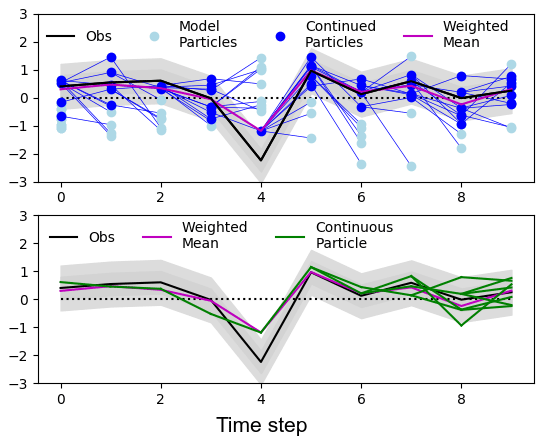
Figure 1Schematic showing the performance of the particle filter. Values are only illustrative and do not represent any particular climate variable. Observations: black with grey uncertainties; model simulations: blue; simulations that are continued: darker blue; weighted mean: purple; continuous simulations: green (note that this quickly converges onto a single simulation as you follow the simulations back in time from the end of the experiment).
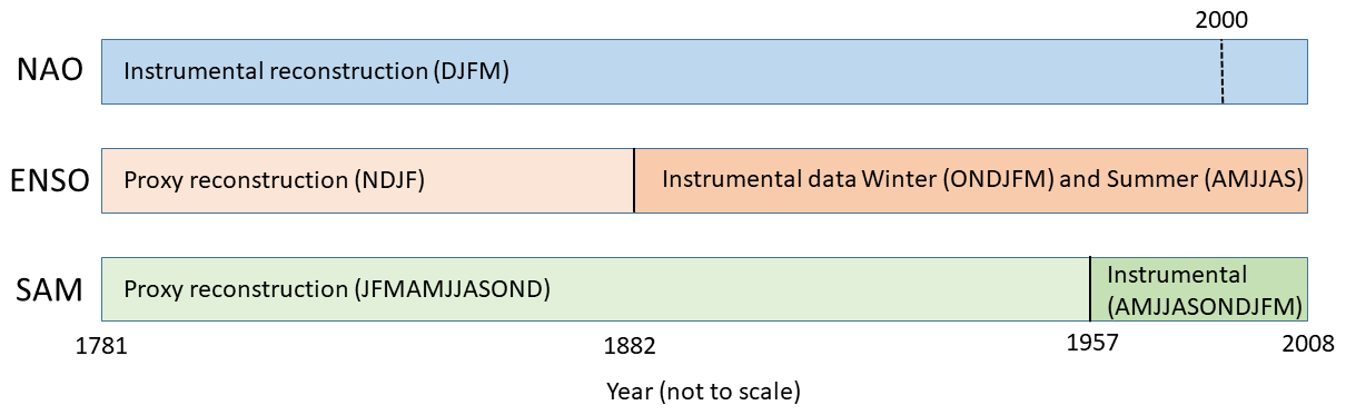
Figure 2Schematic diagram of target indices. The NAO instrumental reconstruction uses Luterbacher et al. (2001) up until the year 2000 and then the 20th-century reanalysis (Compo et al., 2011) thereafter. The ENSO proxy reconstruction uses a combination of Emile-Geay et al. (2013a) and Li et al. (2013) until 1882 and then HadSST3 (Kennedy et al., 2011a, b) thereafter. The SAM proxy reconstruction used is Abram et al. (2014a) until 1957 and then the Marshall index (Marshall, 2003) thereafter.
The indices chosen are shown in Fig. 2. The data used to constrain the data assimilation simulation are intended to be the best available for that particular index. Hence, instrumentally observed indices are used when available and proxy reconstructions when they are not. The consequence of this is that the uncertainty in the target index changes through time, as does the relative uncertainty between the indices and thus the constraint applied to the simulations. The assimilation step was chosen to occur on 1 April, so the simulations are restarted from initial conditions which best agree with the boreal winter, which had just occurred (the period in which the most information is assimilated).
For the NAO index the metric used is the mean of the NAO index over the period December to March and is calculated as the standardised difference between the standardised pressure of the Icelandic Low and the Azores High, as in Luterbacher et al. (2001). For ENSO the metric used is the temperature anomaly over the Niño3.4 region (5∘ N–5∘ S, 170–120∘ W). For 1781–1881 this is the mean over the months November to February and is obtained by the mean of the proxy reconstructions of Li et al. (2013) and Emile-Geay et al. (2013a). In 1882 the metric changes to take advantage of the more reliable instrumental observations (HadSST3; Kennedy et al., 2011a, b), with two periods used, the mean of the Niño3.4 index from April to September and the mean of the index from October to March, to find particles that follow the ENSO evolution during the whole year. The SAM index is initially the annual reconstruction of Abram et al. (2014a). Given that the assimilation occurs on 1 April every year, it means that the first part of the year used to calculate the SAM index is from the previous assimilation step. In 1957 the filter switches to use the instrumental Marshall index (Marshall, 2003). Given that monthly data exist, the mean of the period of April through to March is used to coincide with the assimilation time step, and the metric for this period is calculated as the mean of the monthly values.
Given the finite number of particles (50), none of the individual simulations is capable of perfectly matching all three indices simultaneously. Which index will be given the most weight will be determined by the uncertainty in that particular index (see Eq. 1). The uncertainty associated with each of the indices is shown in the Supplement (Fig. S1). The uncertainties in the proxy reconstructions for the ENSO and particularly the SAM are much larger than the NAO instrumental uncertainty. Thus, the analysis initially tracks the NAO better as the filter preferentially tries to fit this index, as shown by correlations between the assimilated and observed index in Fig. 3 (correlations for the “continuous particle” shown in Fig. S2). Uncertainties in ENSO and then the SAM decrease during the instrumental period (substantially in the case of the SAM); thus the correlation to these indices improves (with the match to the NAO noticeably degrading after 1950). The performance of the filter is also reflected in the number of particles that are re-spawned at each iteration (Fig. S3). This is about 17 till 1881, dropping to 10 when the ENSO instrumental data are used and below 5 when the SAM instrumental data start in 1957. As the number of particles which match the observed indices within their associated uncertainty decreases, more particles are discontinued, and more spawn from the remaining particles. Towards the end of the simulation the filter often only re-spawns from three particles, the minimum allowed. It is important to note that improvement in the agreement on an annual scale is not necessarily related to agreement on a decadal scale as modelled values consistently higher or lower than those observed can lead to large decadal disagreement, for example in the decadally smoothed ENSO index in the mid-20th century (Fig. 3).
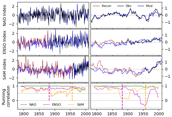
Figure 3Performance of filter. Time series of target indices (top three rows) – NAO (DJFM, climatology period 1782–2008), ENSO (NDJF, climatology period 1882–1992), SAM (annual mean, climatology period 1957–1995) – for the weighted-mean analysis (blue), reconstruction (brown) and instrumental observations (black). Note that because of changes in the target indices through time (Fig. 2), the plotted time series does not always exactly correspond to the data assimilated. Left column panels: annual values; right column panels: annual values smoothed by an 11-year running mean. Bottom left: running 20-year correlation for the annual value; bottom right: 40-year correlations for the decadal values for the NAO (green), ENSO (purple) and SAM (orange). The vertical dashed line shows the switch between proxy and instrumental values for ENSO and SAM.
3.1 Performance validation
The performance of the particle filter experiment is assessed by analysing how well it reproduces the spatial patterns associated with the assimilated indices. The NAO, ENSO and SAM indices were calculated in the observational record and in the particle filter simulation, and in Fig. 4 the sea level pressure fields are regressed on these indices. A comparison of the model pattern (right panels) to the observational counterparts (left panels) can be used to assess whether the HadCM3 climate model is capable of accurately simulating the spatial patterns of these modes of variability. In general the model performs well; however there are some noticeable biases, in particular in the temperature response to ENSO, which is known to extend too far west in HadCM3 (see also Collins et al., 2001), and in the temperature response to the SAM. The central panels show the DA simulation fields regressed on the observed index; the difference between these patterns and the observed regression patterns is shown in the Supplement (Fig. S5). This represents a test of the assimilation procedure. If the particle filter was performing perfectly the modelled indices would be identical to the observed indices, and consequently the central and right panels would be identical. This is almost the case (although the patterns using the observed index are slightly weaker), which is a reflection of the fact that the modelled indices follow the instrumental observations reasonably well, although not perfectly (Fig. 3). Regressing the DA simulation fields on the proxy SAM reconstruction results in a much weaker pattern (not shown), reflecting the loss of performance in this earlier period.
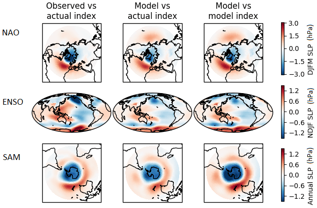
Figure 4Regression between index and sea level pressure. From top to bottom: NAO, ENSO, SAM. Left column: regression between the observed index and the observed spatial pattern of sea level pressure (from 20CRv3; Slivinski et al., 2019). Middle column: regression between the observed index and the DA model spatial pattern. Right column: regression between the DA model index and its own spatial pattern. All data are first detrended. Regressions calculated over the period 1882–2008 except the SAM regressions, which are calculated over the shorter period (1957–2008).
3.2 Correlations of models with observed climate
In order to determine the regions in which the particle filter provides a statistically improved realisation of the observed climate compared to the forcing-only simulations, we estimate skill by using correlation coefficients, as suggested in Goddard et al. (2013). Detrended observed anomalies are correlated with those simulated by the model with and without assimilation for each grid cell to determine where the assimilation is significantly improving the agreement. Because the particle filter results are a weighted mean over a number of particles (see Fig. S3), the internal variability not associated with the three assimilated modes will be reduced. Consequently comparing them directly to each of the forcing-only simulations could give misleading results. To account for this, the average weights which are used in the particle filter experiment for the period analysed are calculated (see Fig. S4) and then applied at random to the 10 forcing-only simulations to create 100 different equivalently weighted means. Results are considered significant if correlations calculated between the observations and the particle filter experiment are greater than 95 % of the equivalent values calculated between the observations and the weighted means from the 10 forcing-only simulations. In order to focus exclusively on the skill gained from including the assimilation, we calculate the difference between the correlation calculated for the assimilated experiment and the mean correlation calculated for the non-assimilated forcing-only simulations (see Fig. 6). In order to provide a test of bias an equivalent figure displaying mean absolute error (instead of the correlation) is shown in Fig. S10. The correlations between the assimilated and non-assimilated model simulations and the observations are shown in the Supplement (Figs. S6 and S7).
Spatial patterns of correlation differences are shown in Fig. 6a and b for annual and boreal-winter (DJF) surface air temperature (the focus is on boreal winter as this is when most data are assimilated; results for other seasons are shown in Fig. S9). In both cases a substantial fraction of the total number of grid squares displays significantly higher correlations than would be expected due to chance. Improved correlations are highest in the central and eastern tropical Pacific due to the effect of ENSO, and regions with strong connections to this mode of variability will show similar behaviour in both models and observations, for example the Indian Ocean and tropical Atlantic (Klein et al., 1999). Outside of the tropics teleconnections to the ENSO variability are much weaker. Other significant increases in correlation (above that expected by chance) are seen in the northern extra-tropics, in the North Atlantic, Europe and Siberia, particularly in winter. This is the region most strongly affected by the NAO (see Hurrell et al., 2003, and Figs. 4 and 5) which is assimilated for this period (December–March). To further investigate correlations over this region we have analysed results using a spatial European reconstruction (Luterbacher et al., 2004) over the full period of the experiment (1782–2000; Fig. 6c and d), in winter and in the annual mean. Correlations are found to be particularly strong over the northern part of Europe in winter, consistent with the effect of the NAO. The effect of the SAM on temperature is not so clear, partly due to limitations in observational coverage. However, there are high and significant correlations in parts of the Southern Ocean, particularly south of Australia and off the southern tip of South America, regions strongly affected by the SAM (see e.g. Fogt and Marshall, 2020) and which have good agreement between models and observations in Fig. 4. The results for mean absolute error (Fig. S10) are broadly similar, showing reduction in bias in the regions which are found to have higher correlations. Note that Fig. 6a–d use the infilled analysis product of HadCRUT5, but the main findings are insensitive to the infilling process (see Fig. S8).
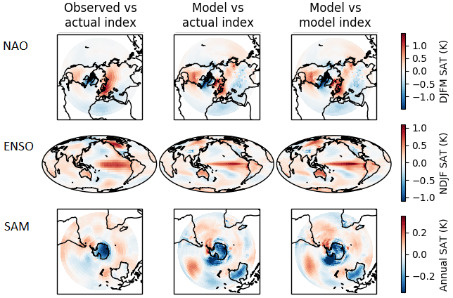
Figure 5Regression between index and surface air temperature. From top to bottom: NAO, ENSO, SAM. Left column: regression between the observed index and the observed spatial pattern of SAT (from HadCRUT5, infilled; Morice et al., 2021). Middle column: regression between the observed index and the DA model spatial pattern. Right column: regression between DA model index and its own spatial pattern. All data are first linearly detrended. Regressions calculated over the period 1882–2008 except the SAM regressions, which are calculated over the shorter period (1957–2008) due to data availability. Grey indicates missing data.
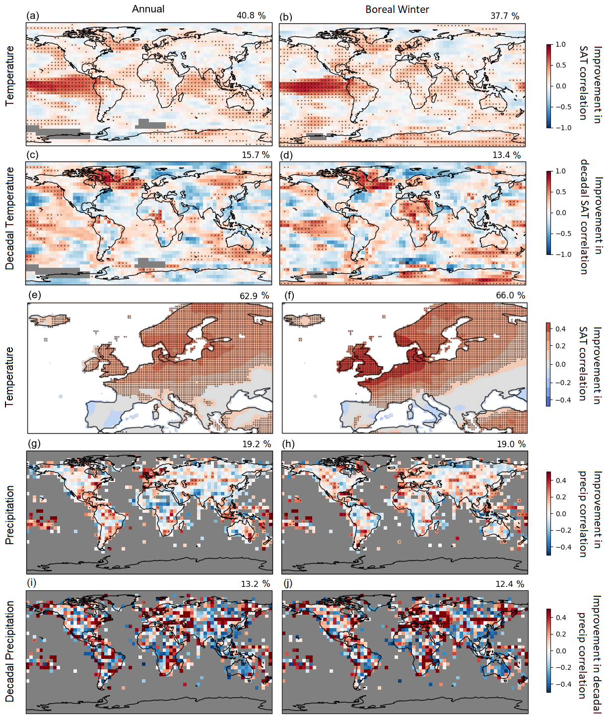
Figure 6Improvement in annual and northern-hemispheric winter (DJF) temperature and precipitation correlation between models and observations due to assimilation. The difference in correlation between observations and the model simulations with and without assimilation. (a, b) Temperature correlations using HadCRUT5 (infilled; Morice et al., 2021) for the period 1882–2008. (c, d) Decadal (11-year running mean) temperature correlations using HadCRUT5 for the period 1882–2008. (e, f) Correlation using a temperature reconstruction (Luterbacher et al., 2004) for the period 1782–2000. (g, h) Correlation using the Global Precipitation Climatology Centre (GPCC) dataset (Schneider et al., 2016) for the period 1950–2008. (i, f) Decadal (11-year running mean) precipitation correlation using GPCC for the period 1950–2008. Stippling indicates where the correlation is bigger than the 95th percentile from the weighted means of the 10 forcing-only model simulations. The number at the top right of every plot indicates the percentage of grid cells which are stippled. If only due to uncorrelated random variability, a value of 5 % would be expected.
Differences in how well the assimilated and forced simulations correlate to observed precipitation are shown in Fig. 6g and h. Due to sparsity in observations the analysis is restricted to land-only regions with a start date of 1950. As for temperature, significant improvements are mainly found in the tropics, particularly in the Pacific, but also in Europe and southern Australia, consistent with the influence of the NAO and the SAM.
One striking aspect of Fig. 6 is that, even for temperature, the assimilation only significantly improves the correlations for about a third of the globe at interannual timescales, with much of the significantly correlated area in the tropics. This is an indication of the relative importance of the three modes of variability assimilated here compared to that of other components of internal variability. At higher latitudes the atmosphere's intrinsic variability is much higher, and although important, the relative role of the indices assimilated here can only explain a relatively small component of the total variability. This demonstrates both the limitations and strengths of this approach; while it will not give as accurate a realisation of past climate as reanalyses which assimilate as much observed daily (or sub-daily) data as possible, it can instead be used to assess the relative role these three indices play in determining the climate.
One interesting aspect is how much variability these indices can explain on a decadal timescale (filtering using a running 11-year mean). As Fig. 6c and d show, the most prominent area of improved correlations on these longer timescales is the North Atlantic, in the sub-polar gyre region, which is an area that has previously been identified as one with a particularly strong link to the NAO and which could play a key role in driving ocean circulation (see e.g. Zhang et al., 2019, for a review). There are also significant correlation improvements in surface temperature on a decadal scale in the Pacific and Indian oceans, over northern Eurasia, in Africa, and in the Southern Ocean. Due to the relatively short period analysed, results for precipitation on a decadal scale are very noisy (Fig. 6i and j). However they do show an increased agreement in the tropical Pacific and in Europe, consistent with the results for surface temperature.
3.3 Large-scale mean climate
Results for correlation against observed large-scale average temperature support the spatial correlations discussed above. The agreement is significantly improved by the assimilation in the global mean and in the tropics and southern-hemispheric extra-tropics (Fig. 7). Temperature in the northern extra-tropics shows an improvement in the particle filter during the second half of the century (particularly north of 35∘ N), with larger correlations than in any simulation without data assimilation, but not during the first half of the century, with values particularly low in the period 1900–1940 and no statistical overall improvement for the period as a whole. A similar result is found in correlations over Europe (Fig. 7h), with very low values at the start of the 20th century. As the NAO has a particularly strong influence on Europe (Hurrell et al., 2003), and the DA model follows the observed NAO closely throughout this period, these weak correlations suggest the effect of the NAO on Europe and northern-high-latitude regions is not constant through time, although uncertainties in observations could also contribute. Other studies (Weisheimer et al., 2019) have also found non-stationarities in the skill of initialised climate models to predict the NAO, with higher values since the 1970s and lower values in the mid-20th century. In general, relatively small improvements in the correlation of temperature at a large scale and over long time periods are expected because at these scales the effect of external forcing will dominate, and much of the discrepancy between simulated and observed climate is likely to be due to errors in the simulated forced response. This is particularly true for higher latitudes, where previous studies have found that, despite a strong regional influence, the NAO only weakly affects large-scale temperatures (Iles and Hegerl, 2017).
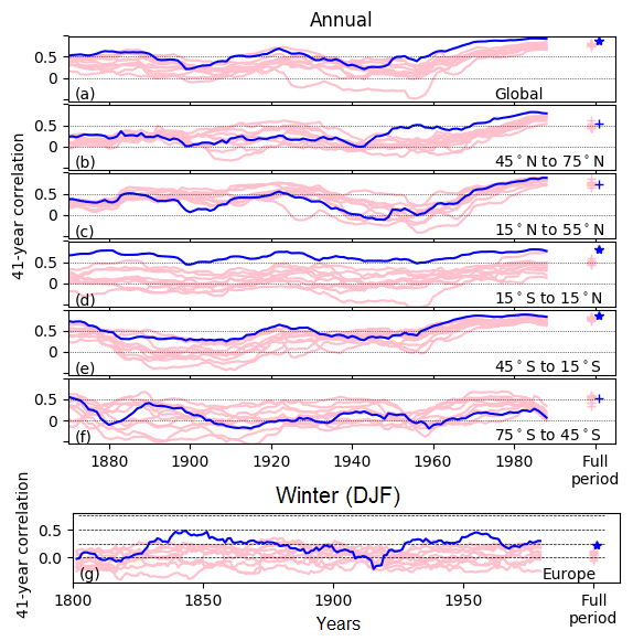
Figure 7The 41-year sliding correlations for annual zonal-mean and European winter air temperature. (a–f) Correlations are calculated between observed and simulated air temperature. (a–f) Correlations between zonal-mean temperatures for latitudes given in the bottom right of each panel between HadCRUT5 (non-infilled) and the forcing-only simulation (pink) and data assimilation simulation (blue). All simulations masked to available observational data coverage. (g) Correlations between a reconstruction of European winter (Luterbacher et al., 2004) and simulations. Correlations over the full period on the right of the plot. If the correlation is greater than all 10 forcing-only simulations, the blue symbol is plotted as a star (instead of a plus).
Previous studies, for example Friedman et al. (2020) and Hegerl et al. (2018), have found that observed decadal temperature variability in the Southern Hemisphere, particularly the extra-tropics, is far greater than that simulated by the latest climate models and is outside the CMIP5 ensemble spread. As we are assimilating the key modes of variability for this region (the ENSO and SAM), it is an interesting question to investigate whether our DA model simulation can offer insights into this discrepancy. Time series of surface air temperatures averaged over zonal bands, including the southern-hemispheric extra-tropics, are shown in Fig. 8. As expected, the observed variability over 65 to 30∘ S is outside the range of the forcing-only simulations. Assimilation does little to improve this situation, suggesting that it is neither the SAM nor the ENSO variability which is responsible for the discrepancy. However, this could partially be due to possible deficiencies in the model's pattern of the SAM (see Figs. 4 and 5). Other intriguing possibilities are limitations in model variability in the Southern Ocean (Hyder et al., 2018), potentially due to the relatively coarse resolution (Beadling et al., 2020), as well as possible biases in SST measurements such as those found in the northern-hemispheric Atlantic and Pacific (Chan et al., 2019) and using coastal weather stations (Cowtan et al., 2018).
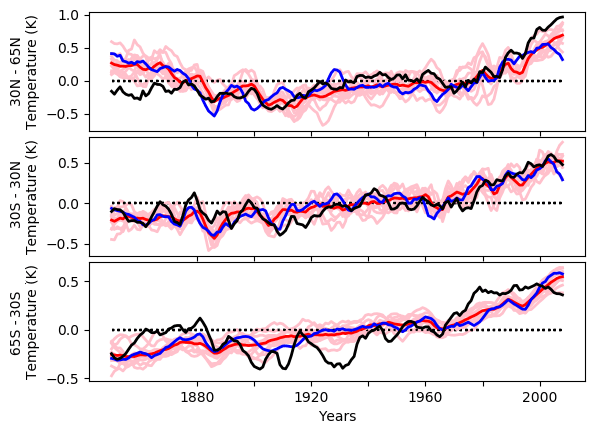
Figure 8Annual-mean surface air temperature averaged over three latitudinal bands. Assimilated model: blue; 10 forcing-only simulations: light pink; forcing-only ensemble mean: red; observations: black (HadCRUT5, non-infilled). All time series are filtered using a 5-year running mean, and simulations are masked to available observational data coverage.
3.4 Temperature response to large volcanic eruptions
Volcanic eruptions have an important role on annual as well as decadal climate (Robock, 2000). However, the global-mean temperature response has been found to be stronger in climate models than in observations (Chylek et al., 2020; Bindoff et al., 2013). It has been suggested that this discrepancy could be explained, at least partially, by ENSO events, which coincide with all major volcanic eruptions during the instrumental era (Lehner et al., 2016), although the role of the volcanic eruption in triggering the occurrence of an El Niño is still disputed (see McGreogor et al., 2020, for a review). Studies of the last millennium which rely on proxy evidence offer mixed results from a longer-term perspective, with some recent studies, typically based on tree-ring evidence, supporting an El Niño-like response in the year following an eruption (e.g. McGregor et al., 2010; Li et al., 2013), while studies based on coral data from the ENSO region itself do not find any significant relationship (Tierney et al., 2015; Dee et al., 2020). Models of different complexities also simulate an El Niño response, although they disagree on the underlying mechanisms (Ohba et al., 2013; Khodri et al., 2017; Predybaylo et al., 2020; Maher et al., 2015; Hermanson et al., 2020). While the majority of studies concentrate on tropical eruptions, modelling studies have also found an important role for high-latitude eruptions, and the mechanism may also be different (Pausata et al., 2015). Given that the data assimilation simulation has been designed to follow the observed ENSO index, it provides an ideal test bed for investigating the effect of the ENSO on the climate after volcanic eruptions, although it cannot provide any evidence to address the question of whether a forced link exists between the eruption and the ENSO state.
To investigate the temperature response following volcanic eruptions we employ a commonly used technique called an epoch analysis (e.g. Hegerl et al., 2003). This involves averaging the response across multiple eruptions in order to reduce internal variability to focus on the forced response. Here we choose the five strongest tropical eruptions which coincide with the period of instrumental observations: Krakatoa (August 1883), Santa Maria (October 1902), Agung (March 1963), El Chichón (April 1982) and Pinatubo (June 1991). The global-mean surface air temperature and Niño3.4 index are calculated for the simulated and observed climate for 60 months after each eruption occurred relative to a pre-eruption mean (calculated as the mean over the 60 months directly before the eruption), and the results for all five are averaged together. Figure 9 shows the results for the epoch analysis for the last five major tropical eruptions. The ENSO index concurrent with the eruptions is on average slightly positive when the volcanic eruptions occur and becomes increasingly positive for the year after the eruptions. This behaviour is captured remarkably well in the DA simulation but not by any of the forcing-only simulations. Based on the results from the forcing-only simulations one would conclude that the model overestimates the response to volcanic eruptions since all model simulations have larger cooling following the eruption than that observed. Assimilating ENSO, however, resolves this clear mismatch, showing that, at least for this model, if a simulation has the correct ENSO evolution the temperature response is very close to that observed.
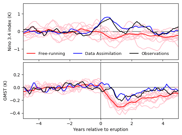
Figure 9Response to five tropical volcanic eruptions. Epoch analysis for observed Niño3.4 SST anomaly index (top) and global-mean surface air temperature (bottom). Observations are HadSST4 (Kennedy et al., 2019) and HadCRUT5 (non-infilled); all simulations are masked to the observations. Both variables are plotted as anomalies from the mean of the 5 years before the eruption date.
In this study, we introduce a new experimental set-up based on existing data assimilation techniques to produce a near-continuous and near-free-running model simulation with a realisation of the ENSO, NAO and SAM similar to that which actually occurred. We have demonstrated that this method adequately captures the assimilated modes and offers an improved realisation of the climate above that of free-running simulations without assimilation in several key regions in both temperature and rainfall. This includes annual- and winter-mean surface temperature over much of the northern extra-tropics, large parts of tropical surface temperature, and tropical and European rainfall. On a decadal scale, improvements in skill are found over much of the tropical Pacific, over some parts of the Southern Ocean and in the sub-polar gyre region of the northern Atlantic. Decadal forecast experiments have shown that the NAO (Smith et al., 2020) and ENSO (Barnston et al., 2019; Dunstone et al., 2020) are predictable on seasonal to annual timescales. This analysis highlights where a prediction system has the potential to better reproduce observed trends if the prediction systems were capable of following the correct realisation of these modes. Interestingly our results also display some evidence of non-stationarity, with the assimilation improving agreement with observations more in some periods than others, suggesting that the skill in decadal forecasts could vary through time.
Past modelling studies have shown that the observations in the southern extra-tropics are far more variable on the decadal scale than model simulations. By assimilating the ENSO and the SAM we can show that getting the evolution of these modes of variability closer to reality does not help to explain this discrepancy. This suggests that the difference must have an alternative origin, such as observational errors or other model deficiencies. Outside this region though, there is no major discrepancy in surface air temperature, providing support for the ability of climate models to reproduce observed climate evolution.
Consistent with most models, the HadCM3 simulations analysed here show too much cooling following volcanic eruptions over the last 150 years. Correctly assimilating ENSO results in simulated cooling that is consistent with the observations. This demonstrates that the model response is not necessarily too strong, but rather the forcing-only simulations do not capture the correct ENSO response. This conclusion highlights that relying on model simulations which do not capture the observed ENSO variability could lead to misleading conclusions.
We therefore consider this use of a particle filter to be a promising experimental design which could be developed further in the future to investigate the causes of past variability or the effect of potential future changes in key circulation modes using a storyline approach. We note that while we have chosen to assimilate three modes of variability in this study, it would be possible to assimilate any number of them. Assimilating fewer modes would reduce the degrees of freedom for the filter and hence allow an improved performance for that mode or alternatively the ability to use fewer particles, while assimilating more has the potential to reduce the performance of the filter unless the number of particles is also increased.
Model simulation data are all publicly available. The particle filter simulation data are available at https://doi.org/10.7488/ds/3829 (Schurer et al., 2023a). The all-forced HadCM3 simulations (without assimilation) are available at https://doi.org/10.7488/ds/3827 (Schurer et al., 2023b). The NAO reconstruction is available at https://crudata.uea.ac.uk/cru/data/paleo/naojurg/ (Climate Research Unit, 2023). The ENSO reconstructions are available at https://doi.org/10.25921/c8ez-6f86 (Li et al., 2011) and https://doi.org/10.25921/t8hf-mt92 (Emile-Geay et al., 2013b). The SAM reconstruction is available at https://doi.org/10.25921/3egm-zr66 (Abram et al., 2014b). The seasonal European temperature reconstruction is available at https://doi.org/10.25921/1hw9-nz71 (Luterbacher et al., 2006). The Marshall index is available at https://legacy.bas.ac.uk/met/gjma/sam.html (BAS, 2023). HadSST3 is available at https://www.metoffice.gov.uk/hadobs/hadsst3/ (Met Office, 2011). HadSST4 is available at https://www.metoffice.gov.uk/hadobs/hadsst4/ (Met Office, 2019). HadCRUT5 is available at https://www.metoffice.gov.uk/hadobs/hadcrut5/ (Met Office, 2021). GPCC is available at https://doi.org/10.5676/DWD_GPCC/FD_M_V2020_250 (Schneider et al., 2020).
The supplement related to this article is available online at: https://doi.org/10.5194/cp-19-943-2023-supplement.
The contact author has declared that none of the authors has any competing interests.
APS, GCH and HG designed the study. APS and MJM set up the climate model experimental design with support from HG and SFBT. APS ran the model simulations and conducted all analysis. APS, GCH, HG, MAB, MHE, MJM, DMS, and SFBT contributed to the manuscript writing.
Publisher's note: Copernicus Publications remains neutral with regard to jurisdictional claims in published maps and institutional affiliations.
The model simulations and Andrew P. Schurer, Gabriele C. Hegerl, Michael J. Mineter and Simon F. B. Tett were funded by the ERC-funded project TITAN (EC-320691) and made use of the resources provided by the Edinburgh Compute and Data Facility (ECDF) (http://www.ecdf.ed.ac.uk/, last access: 6 March 2019). Andrew P. Schurer and Gabriele C. Hegerl were further supported by the JPI-Belmont project “PAleao-Constraints on Monsoon Evolution and Dynamics (PACMEDY)” through the UK Natural Environmental Research Council (NERC) (NE/P006752/1), the NERC projects GloSAT (NE/S015698/1) and Vol-Clim (NE/S000887/1), and Andrew P. Schurer received funding from a Chancellor's Fellowship at the University of Edinburgh. Doug M. Smith was supported by the Met Office Hadley Centre Climate Programme funded by BEIS and Defra. Hugues Goosse is research director at the Fonds de la Recherche Scientifique (F. R. S.-FNRS). MHE was supported by the Australian Research Council (SR200100008). We are grateful to the reviewers for insightful comments that improved the manuscript and its presentation and to the editor for helpful direction.
This research has been supported by the European Research Council, FP7 Ideas: European Research Council (TITAN; grant no. 320691) and the Natural Environment Research Council (grant nos. NE/P006752/1, NE/S015698/1 and NE/S000887/1).
This paper was edited by Nerilie Abram and reviewed by two anonymous referees.
Abram, N. J., Mulvaney, R., Vimeux, F., Phipps, S. J., Turner, J., and England, M. H.: Evolution of the Southern Annular Mode during the Past Millennium, Nat. Clim. Change, 4, 564–569, https://doi.org/10.1038/nclimate2235, 2014a.
Abram, N. J., Mulvaney, R., Vimeux, F., Phipps, S. J., Turner, J., and England, M. H.: NOAA/WDS Paleoclimatology – Southern Annular Mode 1000 Year Reconstruction, NOAA National Centers for Environmental Information [data set], https://doi.org/10.25921/3egm-zr66, 2014b.
Allen, M. R. and. Stott P. A.: Estimating Signal Amplitudes in Optimal Fingerprinting, Part I: Theory, Clim. Dynam., 21, 477–491, https://doi.org/10.1007/s00382-003-0313-9, 2003.
Barnston, A. G., Tippett, M. K., Ranganathan, M., and L'Heureux, M. L.: Deterministic Skill of ENSO Predictions from the North American Multimodel Ensemble, Clim. Dynam., 53, 7215–7234, https://doi.org/10.1007/S00382-017-3603-3, 2019.
BAS – British Antarctic Survey: An observation-based Southern Hemisphere Annular Mode Index, BAS [data set], https://legacy.bas.ac.uk/met/gjma/sam.html (last access: 5 May 2023), 2023.
Beadling, R. L., Russell, J. L., Stouffer, R. J., Mazloff, M., Talley, L. D., Goodman, P. J., Sallée, J. B., Hewitt, H. T., Hyder, P., and Pandde, A.: Representation of Southern Ocean Properties across Coupled Model Intercomparison Project Generations: CMIP3 to CMIP6, J. Climate, 33, 6555–6581, https://doi.org/10.1175/JCLI-D-19-0970.1, 2020.
Bindoff, N. L., Stott, P. A., AchutaRao, K. M., Allen, M. R., Gillett, N., Gutzler, D., Hansingo, K., Hegerl, G., Hu, Y., Jain, S., Mokhov, I. I., Overland, J., Perlwitz, J., Sebbari, R., and Zhang, X.: Detection and Attribution of Climate Change: from Global to Regional, in: Climate Change 2013: The Physical Science Basis, Contribution of Working Group I to the Fifth Assessment Report of the Intergovernmental Panel on Climate Change, edited by: Stocker, T. F., Qin, D., Plattner, G.-K., Tignor, M., Allen, S. K., Boschung, J., Nauels, A., Xia, Y., Bex, V., and Midgley, P. M., Cambridge University Press, Cambridge, UK and New York, NY, USA, https://doi.org/10.1017/CBO9781107415324.022, 2013.
Brönnimann, S., Franke, J., Nussbaumer, S. U., Zumbühl, H. J., Steiner, D., Trachsel, M., Hegerl, G. C., Schurer, A., Worni, M., Malik, A., Flückiger, J., and Raible, C. C.: Last Phase of the Little Ice Age Forced by Volcanic Eruptions, Nat. Geosci., 12, 650–656, https://doi.org/10.1038/s41561-019-0402-y, 2019.
Brunner, L., McSweeney, C., Ballinger, A. P., Befort, D. J., Benassi, M., Booth, B., Coppola, E., de Vries, H., Harris, G., Hegerl, G. C., Knutti, R., Lenderink, G., Lowe, J., Nogherotto, R., O'Reilly, C., Qasmi, S., Ribes, A., Stocchi, P., and Undorf, S.: Comparing Methods to Constrain Future European Climate Projections Using a Consistent Framework, J. Climate, 33, 8671–8692, https://doi.org/10.1175/JCLI-D-19-0953.1, 2020.
Cai, W., Wang, G., Santoso, A., McPhaden, M. J., Wu, L., Jin, F., Timmermann, A., Collins, M., Vecchi, G., Lengaigne, M., England, M. H., Dommenget, D., Takahashi, K., and Guilyardi, E.: Increased Frequency of Extreme La Niña Events under Greenhouse Warming, Nat. Clim. Change, 5, 132–137, https://doi.org/10.1038/nclimate2492, 2015.
Chen, D. and Cane. M. A.: El Niño Prediction and Predictability, J. Comput. Phys., 227, 3625–3640, https://doi.org/10.1016/J.JCP.2007.05.014, 2008.
Chylek, P., Folland, C., Klett, J. D., and Dubey, M. K.: CMIP5 Climate Models Overestimate Cooling by Volcanic Aerosols, Geophys. Res. Lett., 47, e2020GL087047, https://doi.org/10.1029/2020GL087047, 2020.
Climate Research Unit: Luterbacher et al NAO Reconstructions back to 1500, https://crudata.uea.ac.uk/cru/data/paleo/naojurg/ (last access: 5 May 2023), 2023.
Collins, M., Tett, S. F. B., and Cooper, C.: The Internal Climate Variability of HadCM3, a Version of the Hadley Centre Coupled Model without Flux Adjustments, Clim. Dynam., 17, 61–81, https://doi.org/10.1007/S003820000094, 2001.
Collins, M., Knutti, R., Arblaster, J., Dufresne, J.-L., Fichefet, T., Friedlingstein, P., Gao, X., Gutowski, W. J., Johns, T., Krinner, G., Shongwe, M., Tebaldi, C., Weaver, A. J., and Wehner, M.: Long-term Climate Change: Projections, Commitments and Irreversibility, in: Climate Change 2013: The Physical Science Basis, Contribution of Working Group I to the Fifth Assessment Report of the Intergovernmental Panel on Climate Change, edited by: Stocker, T. F., Qin, D., Plattner, G.-K., Tignor, M., Allen, S. K., Boschung, J., Nauels, A., Xia, Y., Bex, V., and Midgley, P. M., Cambridge University Press, Cambridge, UK and New York, NY, USA, https://doi.org/doi:10.1017/CBO9781107415324.024, 2013.
Compo, G., Whitaker, J., Sardeshmukh, P., Matsui, N., Allan, R., Yin, A., Gleason, B., Vose, R., Rutledge, G., Bessemoulin, P., Brönnimann, S., Brunet, M., Crouthamel, R., Grant, A., Groisman, P., Jones, P., Kruk, M., Kruger, A., Marshall, G., Maugeri, M., Mok, H., Nordli, Ø., Ross, T., Trigo, R., Wang, X., Woodruff, S., and Worley, S.: The twentieth century reanalysis project, Q. J. Roy. Meteorol. Soc., 137, 1–28, https://doi.org/10.1002/qj.776, 2011.
Cowtan, K., Rohde, R., and Hausfather, Z.: Evaluating Biases in Sea Surface Temperature Records Using Coastal Weather Stations, Q. J. Roy. Meteorol. Soc., 144, 670–681, https://doi.org/10.1002/qj.3235, 2018.
Dee, S. G., Cobb, K. M. Emile-Geay, J., Ault, T. R., Lawrence Edwards, R., Cheng, H., and Charles, C. D.: No Consistent ENSO Response to Volcanic Forcing over the Last Millennium, Science, 367, 1477–1481, https://doi.org/10.1126/SCIENCE.AAX2000, 2020.
Delworth, T. L. and Zeng, F.: The Impact of the North Atlantic Oscillation on Climate through Its Influence on the Atlantic Meridional Overturning Circulation, J. Climate, 29, 941–962, https://doi.org/10.1175/JCLI-D-15-0396.1, 2016.
Delworth, T. L., Zeng, F., Vecchi, G. A., Yang, X., Zhang, L., and Zhang, R.: The North Atlantic Oscillation as a Driver of Rapid Climate Change in the Northern Hemisphere, Nat. Geosci., 9, 509–512, https://doi.org/10.1038/ngeo2738, 2016.
Deser, C., Phillips, A., Bourdette, V., and Teng, H.: Uncertainty in Climate Change Projections: The Role of Internal Variability, Clim. Dynam., 38, 527–546, https://doi.org/10.1007/S00382-010-0977-X, 2012.
Deser, C., Lehner, F., Rodgers, K. B., Ault, T., Delworth, T. L., DiNezio, P. N., Fiore, A., Frankignoul, C., Fyfe, J. C., Horton, D. E., Kay, J. E., Knutti, R., Lovenduski, N. S., Marotzke, J., McKinnon, K. A., Minobe, S., Randerson, J., Screen, J. A., Simpson, I. R., and Ting, M.:: Insights from Earth System Model Initial-Condition Large Ensembles and Future Prospects, Nat. Clim. Change, 10, 277–286, https://doi.org/10.1038/s41558-020-0731-2, 2020.
Dubinkina, S., Goosse, H., Sallaz-Damaz, Y., Crespin, E., and Crucifix, M.: Testing a Particle Filter to Reconstruct Climate Changes over the Past Centuries, Int. J. Bifurcat. Chaos, 21, 3611–3618, https://doi.org/10.1142/S0218127411030763, 2011.
Dunstone, N., Smith, D., Yeager, S., Danabasoglu, G., Monerie, P., Hermanson, L., Eade, R., Ineson, S., Robson, J., Scaife, A., and Ren, H. L.: Skilful Interannual Climate Prediction from Two Large Initialised Model Ensembles, Environ. Res. Lett., 15, 094083, https://doi.org/10.1088/1748-9326/AB9F7D, 2020.
Duo, C., Kent, E. C., Berry, D. I., and Huybers, P.: Correcting Datasets Leads to More Homogeneous Early-Twentieth-Century Sea Surface Warming, Nature, 571, 393–397, https://doi.org/10.1038/s41586-019-1349-2, 2019.
Emile-Geay, J., Cobb, K. M., Mann, M. E., and Wittenberg, A. T.: Estimating Central Equatorial Pacific SST Variability over the Past Millennium. Part II: Reconstructions and Implications, J. Climate, 26, 2329–2352, https://doi.org/10.1175/JCLI-D-11-00511.1, 2013.
Emile-Geay, J., Cobb, K. M., Mann, M. E., and Wittenberg, A. T.: NOAA/WDS Paleoclimatology – Central Equatorial Pacific NINO3.4 850 Year SST Reconstructions, NOAA National Centers for Environmental Information [data set], https://doi.org/10.25921/t8hf-mt92, 2013b.
Eyring, V., Bony, S., Meehl, G. A., Senior, C. A., Stevens, B., Stouffer, R. J., and Taylor, K. E.: Overview of the Coupled Model Intercomparison Project Phase 6 (CMIP6) Experimental Design and Organization, Geosci. Model Deve., 9, 1937–1958, https://doi.org/10.5194/gmd-9-1937-2016, 2016.
Eyring, V., Gillett, N. P., Achuta Rao, K. M., Barimalala, R., Barreiro Parrillo, M., Bellouin, N., Cassou, C., Durack, P. J., Kosaka, Y., McGregor, S., Min, S., Morgenstern, O., and Sun, Y.: Human Influence on the Climate System, in:Climate Change 2021: The Physical Science Basis, Contribution of Working Group I to the Sixth Assessment Report of the Intergovernmental Panel on Climate Change, edited by: Masson-Delmotte, V., Zhai, P., Pirani, A., Connors, S. L., Péan, C., Berger, S., Caud, N., Chen, Y., Goldfarb, L., Gomis, M. I., Huang, M., Leitzell, K., Lonnoy, E., Matthews, J. B. R., Maycock, T. K., Waterfield, T., Yelekçi, O., Yu, R., and Zhou, B., Cambridge University Press, Cambridge, UK and New York, NY, USA, 423–552, https://doi.org/10.1017/9781009157896.005, 2021.
Flato, G., Marotzke, J., Abiodun, B., Braconnot, P., Chou, S. C., Collins, W., Cox, P., Driouech, F., Emori, S., Eyring, V., Forest, C., Gleckler, P., Guilyardi, E., Jakob, C., Kattsov, V., Reason, C., and Rummukainen, M.: Evaluation of Climate Models, in: Climate Change 2013: The Physical Science Basis, Contribution of Working Group I to the Fifth Assessment Report of the Intergovernmental Panel on Climate Change, edtited by: Stocker, T. F., Qin, D., Plattner, G.-K., Tignor, M., Allen, S. K., Boschung, J., Nauels, A., Xia, Y., Bex, V., and Midgley, P. M., Cambridge University Press, Cambridge, UK and New York, NY, USA, https://doi.org/10.1017/CBO9781107415324.020, 2013.
Fogt, R. L. and Marshall, G. J.: The Southern Annular Mode: Variability, Trends, and Climate Impacts across the Southern Hemisphere, Wiley Interdisciplin. Rev.: Clim. Change, 11, e652, https://doi.org/10.1002/WCC.652, 2020.
Franke, J., Brönnimann, S., Bhend, J., and Brugnara, Y.: A Monthly Global Paleo-Reanalysis of the Atmosphere from 1600 to 2005 for Studying Past Climatic Variations, Scient. Data, 4, 170076, https://doi.org/10.1038/sdata.2017.76, 2017.
Friedman, A. R., Hegerl, G. C., Schurer, A. P., Lee, S., Kong, W., Cheng, W., and Chiang. J. C. H.: Forced and Unforced Decadal Behavior of the Interhemispheric SST Contrast during the Instrumental Period (1881–2012): Contextualizing the Late 1960s–Early 1970s Shift, J. Climate, 33, 3487–3509, https://doi.org/10.1175/JCLI-D-19-0102.1, 2020.
Gillett, N. P., Kirchmeier-Young, M., Ribes, A., Shiogama, H., Hegerl, G. C., Knutti, R., Gastineau, G., John, J. G., Li, L., Nazarenko, L., Rosenbloom, N., Seland, Ø., Wu, T., Yukimoto, S., and Ziehn, T.: Constraining Human Contributions to Observed Warming since the Pre-Industrial Period, Nat. Clim. Change, 11, 207–212, https://doi.org/10.1038/s41558-020-00965-9, 2021.
Goddard, L., Kumar, A., Solomon, A., Smith, D., Boer, G., Gonzalez, P., Kharin, V., Merryfield M., Deser, C., Mason, S., Kirtman, B., Msadek, R., Sutton, R., Hawkins, E., Fricker, T., Hegerl G., Ferro, C., Stephenson, D., Meehl, G., Stockdale, T., Burgman, R., Greene, A., Kushnir, Y., Newman, M., Carton, J., Fukumori, I., and Delworth, T.: A Verification Framework for Interannual-to-Decadal Predictions Experiments, Clim. Dynam., 40, 245–272, https://doi.org/10.1007/S00382-012-1481-2, 2013.
Goosse, H., Crespin, E., Dubinkina, S., Loutre, M., Mann, M. E., Renssen, H., Sallaz-Damaz, Y., and Shindell, D.: The Role of Forcing and Internal Dynamics in Explaining the `Medieval Climate Anomaly', Clim. Dynam., 39, 2847–2866, https://doi.org/10.1007/s00382-012-1297-0, 2012.
Gordon, C., Cooper, C., Senior, C. A., Banks, H., Gregory, J. M., Johns, T. C., Mitchell, J. F. B., and Wood, R. A.: The Simulation of SST, Sea Ice Extents and Ocean Heat Transports in a Version of the Hadley Centre Coupled Model without Flux Adjustments, Clim. Dynami., 16, 147–168, https://doi.org/10.1007/s003820050010, 2000.
Hakim, G. J., Emile-Geay, J., Steig, E. J., Noone, D., Anderson, D. M., Tardif, R., Steiger, N., and Perkins, W. A.: The Last Millennium Climate Reanalysis Project: Framework and First Results, J. Geophys. Res.-Atmos., 121, 6745–676, https://doi.org/10.1002/2016JD024751, 2016.
Hartmann, D. L., Klein Tank, A. M. G., Rusticucci, M., Alexander, L. V., Brönnimann, S., Charabi, Y., Dentener, F. J., Dlugokencky, E. J., Easterling, D. R., Kaplan, A., Soden, B. J., Thorne, P. W., Wild, M., and Zhai, P. M.: Observations: Atmosphere and Surface, in: Climate Change 2013: The Physical Science Basis, Contribution of Working Group I to the Fifth Assessment Report of the Intergovernmental Panel on Climate Change, edited by: Stocker, T. F., Qin, D., Plattner, G.-K., Tignor, M., Allen, S. K., Boschung, J., Nauels, A., Xia, Y., Bex, V., and Midgley, P. M., Cambridge University Press, Cambridge, UK and New York, NY, USA, https://doi.org/10.1017/CBO9781107415324.008, 2013.
Hawkins, E. and Sutton, R.: The Potential to Narrow Uncertainty in Regional Climate Predictions, B. Am. Meteorol. Soc., 90, 1095–1108, https://doi.org/10.1175/2009BAMS2607.1, 2009.
Hegerl, G. and Zwiers, F.: Use of models in detection and attribution of climate change, WIREs Clim. Change, 2, 570–591, https://doi.org/10.1002/wcc.121, 2011.
Hegerl, G. C., Crowley, T. J., Baum, S. K., Kim, K., and Hyde, W. T.: Detection of Volcanic, Solar and Greenhouse Gas Signals in Paleo-Reconstructions of Northern Hemispheric Temperature, Geophys. Res. Lett., 30, 1242, https://doi.org/10.1029/2002GL016635, 2003.
Hegerl, G. C., Brönnimann, S., Schurer, A., and Cowan, T.: The Early 20th Century Warming: Anomalies, Causes, and Consequences, Wiley Interdisciplin. Rev.: Clim. Change, 9, e522, https://doi.org/10.1002/wcc.522, 2018.
Hermanson, L., Bilbao, R., Dunstone, N., Ménégoz, M., Ortega, P., Pohlmann, H., Robson, J. I., Smith, D. M., Strand, G., Timmreck, C., Yeager, S., and Danabasoglu, G.: Robust Multiyear Climate Impacts of Volcanic Eruptions in Decadal Prediction Systems, J. Geophys. Res.-Atmos., 125, e2019JD031739, https://doi.org/10.1029/2019JD031739, 2020.
Hurrell, J. W., Kushnir, Y., Ottersen, G., and Visbeck, M.: An Overview of the North Atlantic Oscillation, Geophys. Monogr. Ser., 134, 1–35, https://doi.org/10.1029/134GM01, 2003.
Hyder, P., Edwards, J. M., Allan, R. P., Hewitt, H. T., Bracegirdle, T. J., Gregory, J. M., Wood, R. A., Meijers, A. J. S., Mulcahy, J., Field, P., Furtado, K., Bodas-Salcedo, A., Williams, K. D., Copsey, D., Josey, S. A., Liu, C., Roberts, C. D., Sanchez, C., Ridley, J., Thorpe, L., Hardiman, S. C., Mayer, M., Berry, D. I., and Belcher, S. E.: Critical Southern Ocean Climate Model Biases Traced to Atmospheric Model Cloud Errors, Nat. Commun., 9, 3625, https://doi.org/10.1038/s41467-018-05634-2, 2018.
Iles, C. and Hegerl, G. C.: Role of the North Atlantic Oscillation in Decadal Temperature Trends, Environ. Res. Lett., 12, 114010, https://doi.org/10.1088/1748-9326/aa9152, 2017.
Kennedy, J. J., Rayner, N. A., Smith, R. O., Parker, D. E., and Saunby, M.: Reassessing biases and other uncertainties in sea surface temperature observations measured in situ since 1850: 1. Measurement and sampling uncertainties, J. Geophys. Res.-Atmos., 116, D14103, https://doi.org/10.1029/2010JD015218, 2011a.
Kennedy, J. J., Rayner, N. A., Smith, R. O., Parker, D. E., and Saunby, M.: Reassessing biases and other uncertainties in sea surface temperature observations measured in situ since 1850: 2. Biases and homogenization, J. Geophys. Res.-Atmos., 116, D14104, https://doi.org/10.1029/2010JD015220, 2011b.
Kennedy, J. J., Rayner, N. A., Atkinson, C. P., and Killick, R. E.: An ensemble data set of sea surface temperature change from 1850: The Met Office Hadley Centre HadSST.4.0.0.0 data set, J. Geophys. Res.-Atmos., 124, 7719–7763, https://doi.org/10.1029/2018JD029867, 2019.
Kettleborough, J. A., Booth, B. B. B., Stott, P. A., and Allen, M. R.: Estimates of Uncertainty in Predictions of Global Mean Surface Temperature, J. Climate, 20, 843–855, https://doi.org/10.1175/JCLI4012.1, 2007.
Khodri, M., Izumo, T., Vialard, J., Janicot, S., Cassou, C., Lengaigne, M., Mignot, J., Gastineau, G., Guilyardi, E., Lebas, N., Robock, A., and McPhaden, M.: Tropical Explosive Volcanic Eruptions Can Trigger El Niño by Cooling Tropical Africa, Nat. Commun., 8, 1–13, https://doi.org/10.1038/s41467-017-00755-6, 2017.
Klein, S. A., Soden, B. J., and Lau, N. C.: Remote Sea Surface Temperature Variations during ENSO: Evidence for a Tropical Atmospheric Bridge, Journal Climate, 12, 917–932, https://doi.org/10.1175/1520-0442(1999)012<0917:RSSTVD>2.0.CO;2, 1999.
Knight, J. R.: A Signature of Persistent Natural Thermohaline Circulation Cycles in Observed Climate, Geophys. Res. Lett., 32, L20708, https://doi.org/10.1029/2005GL024233, 2005.
Knutti, R., Masson, D., and Gettelman, A.: Climate Model Genealogy: Generation CMIP5 and How We Got There, Geophys. Res. Lett., 40, 1194–1199, https://doi.org/10.1002/grl.50256, 2013.
Kosaka, Y. and Xie. S.: Recent Global-Warming Hiatus Tied to Equatorial Pacific Surface Cooling, Nature, 501, 403–407, https://doi.org/10.1038/nature12534, 2013.
Lehner, F., Schurer, A. P., Hegerl, G. C., Deser, C., and Frölicher, T. L.: The Importance of ENSO Phase during Volcanic Eruptions for Detection and Attribution, Geophys. Res. Lett., 43, 2851–2858, https://doi.org/10.1002/2016GL067935, 2016.
Lehner, F., Deser, C., Maher, N., Marotzke, J., Fischer, E. M., Brunner, L., Knutti, R., and Hawkins, E.: Partitioning Climate Projection Uncertainty with Multiple Large Ensembles and CMIP5/6, Earth Syst. Dynam., 11, 491–508, https://doi.org/10.5194/esd-11-491-2020, 2020.
Li, J., Xie, S.-P., Cook, E. R., Huang, G., D'Arrigo, R. D., Liu, F., Ma, J., and Zheng, X.-T.: NOAA/WDS Paleoclimatology – 1,100 Year El Niño/Southern Oscillation (ENSO) Index Reconstruction, NOAA National Centers for Environmental Information [data set], https://doi.org/10.25921/c8ez-6f86, 2011.
Li, J., Xie, S. P., Cook, E. R., Morales, M. S., Christie, D. A., Johnson, N. C., Chen, F., D'Arrigo, R., Fowler, A. M., Gou, X., and Fang, K.: El Niño Modulations over the Past Seven Centuries, Nat. Clim. Change, 3, 822–826, https://doi.org/10.1038/nclimate1936, 2013.
Luterbacher, J., Xoplaki, E., Dietrich, D., Jones, P. D., Davies, T. D., Portis, D., Gonzalez-Rouco, J. F., Von Storch, H., Gyalistras, D., Casty, C., and Wanner, H.: Extending North Atlantic Oscillation Reconstructions Back to 1500, Atmos. Sci. Lett., 2, 114–124, https://doi.org/10.1006/asle.2001.0044, 2001.
Luterbacher, J., Dietrich, D., Xoplaki, E., Grosjean, M., and Wanner, H.: European seasonal and annual temperature variability, trends, and extremes since 1500, Science, 303, 1499–1503, https://doi.org/10.1126/science.1093877, 2004.
Luterbacher, J., Dietrich, D., Xoplaki, E., Grosjean, M., Wanner, H., Paeth, H., and Steiner, N.: NOAA/WDS Paleoclimatology – Xoplaki 2005, Luterbacher 2004 European Seasonal Temperature Reconstructions, NOAA National Centers for Environmental Information [data set], https://doi.org/10.25921/1hw9-nz71, 2006.
Maher, N., McGregor, S., England, M. H., and Gupta, A. S.: Effects of Volcanism on Tropical Variability, Geophys. Res. Lett., 42, 6024–6033, https://doi.org/10.1002/2015GL064751, 2015.
Maher, N., Milinski, S., and Ludwig, R.: Large Ensemble Climate Model Simulations: Introduction, Overview, and Future Prospects for Utilising Multiple Types of Large Ensemble, Earth Syst. Dynam., 12, 401–418, https://doi.org/10.5194/esd-12-401-2021, 2021.
Marshall, G. J.: Trends in the Southern Annular Mode from Observations and Reanalyses, J. Climate, 16, 4134–4143, https://doi.org/10.1175/1520-0442(2003)016<4134:TITSAM>2.0.CO;2, 2003.
McGregor, S., Timmermann, A., and Timm, O.: A Unified Proxy for ENSO and PDO Variability since 1650, Clim. Past, 6, 1–17, https://doi.org/10.5194/cp-6-1-2010, 2010.
McGregor, S., Khodri, M., Maher, N., Ohba, M., Pausata, F. S. R., and Stevenson, S.: The effect of strong volcanic eruptions on ENSO, in: El Niño southern oscillation in a changing climate, Geophysical Monograph Series, American Geophysical Union, 267–287, https://doi.org/10.1002/9781119548164.ch12, 2020.
Met Office: Hadley Centre SST data set (HadSST3) now deprecated, Met Office [data set], https://www.metoffice.gov.uk/hadobs/hadsst3/ (last access: 5 May 2023), 2011.
Met Office: HadSST.4.0.1.0, Met Office [data set], https://www.metoffice.gov.uk/hadobs/hadsst4/ (last access: 5 May 20230, 2019.
Met Office: HadCRUT5, Met Office [data set], https://www.metoffice.gov.uk/hadobs/hadcrut5/ (last access: 5 May 2023), 2021.
Morice, C. P., Kennedy, J. J., Rayner, N. A., Winn, J. P., Hogan, E., Killick, R. E., Dunn, R. J. H., Osborn, T. J., Jones, P. D., and Simpson, I. R.: An Updated Assessment of Near-Surface Temperature Change From 1850: The HadCRUT5 Data Set, J. Geophys. Res.-Atmos., 126, e2019JD032361, https://doi.org/10.1029/2019JD032361, 2021.
Ohba, M., Shiogama, H., Yokohata, T., and Watanabe, M.: Impact of Strong Tropical Volcanic Eruptions on ENSO Simulated in a Coupled GCM, J. Climate, 26, 5169–5182, https://doi.org/10.1175/JCLI-D-12-00471.1, 2013.
Olonscheck, D., Schurer, A. P., Lücke, L., and Hegerl, G. C.: Large-Scale Emergence of Regional Changes in Year-to-Year Temperature Variability by the End of the 21st Century, Nat. Commun., 12, 1–10, https://doi.org/10.1038/s41467-021-27515-x, 2021.
Pausata, F. S. R., Chafik, L., Caballero, R., and Battisti, D. S.: Impacts of High-Latitude Volcanic Eruptions on ENSO and AMOC, P. Natl. Acad. Sci. USA, 112, 13784–13788, https://doi.org/10.1073/PNAS.1509153112, 2015.
Pope, V. D., Gallani, M. L., Rowntree, P. R., and Stratton, R. A.: The Impact of New Physical Parametrizations in the Hadley Centre Climate Model: HadAM3, Clim. Dynam., 16, 123–146, https://doi.org/10.1007/s003820050009, 2000.
Predybaylo, E., Stenchikov, G., Wittenberg, A. T., and Osipov S.: El Niño/Southern Oscillation Response to Low-Latitude Volcanic Eruptions Depends on Ocean Pre-Conditions and Eruption Timing, Commun. Earth Environ., 1, 1–13, https://doi.org/10.1038/s43247-020-0013-y, 2020.
Ribes, A., Zwiers, F. W., Azaïs, J., and Naveau, P.: A New Statistical Approach to Climate Change Detection and Attribution, Clim. Dynam., 48, 367–386, https://doi.org/10.1007/s00382-016-3079-6, 2017.
Robock, A.: Volcanic Eruptions and Climate, Rev. Geophys., 38, 191–219, https://doi.org/10.1029/1998RG000054, 200.
Sanderson, B. M., Knutti, R., and Caldwell, P.: Addressing Interdependency in a Multimodel Ensemble by Interpolation of Model Properties, J. Climate, 28, 5150–5170, https://doi.org/10.1175/JCLI-D-14-00361.1, 2015.
Schneider, U., Ziese, M., Meyer-Christoffer, A., Finger, P., Rustemeier, E., and Becker, A.: The New Portfolio of Global Precipitation Data Products of the Global Precipitation Climatology Centre Suitable to Assess and Quantify the Global Water Cycle and Resources, P. Natl. Acad. Sci. USA, 374, 29–34, https://doi.org/10.5194/PIAHS-374-29-2016, 2016.
Schneider, U., Becker, A., Finger, P., Rustemeier, E., and Ziese, M.: GPCC Full Data Monthly Product Version 2020 at 2.5∘: Monthly Land-Surface Precipitation from Rain-Gauges built on GTS-based and Historical Data, Deutscher Wetterdienst [data set], https://doi.org/10.5676/DWD_GPCC/FD_M_V2020_250, 2020.
Schurer, A., Mineter, M., Hegerl, G., Goosse, H., Bollasina, M., England, M., Smith, D., and Tett, S.: Particle filter HadCM3 simulation, 1781–2008, University of Edinburgh, School of GeoSciences [data set], https://doi.org/10.7488/ds/3829, 2023a.
Schurer, A., Mineter, M., and Tett, S.: 10 member ensemble of HadCM3 simulations, 1780–2009, University of Edinburgh, School of GeoSciences [data set], https://doi.org/10.7488/ds/3827, 2023b.
Schurer, A. P., Tett, S. F. B., and Hegerl, G. C.: Small Influence of Solar Variability on Climate over the Past Millennium, Nat. Geosci., 7, 104–108, https://doi.org/10.1038/ngeo2040, 2014.
Slivinski, L. C., Compo, G. P., Whitaker, J. S., Sardeshmukh, P. D., Giese, B. S., McColl, C., Allan, R., Yin, X., Vose, R., Titchner, H., Kennedy, J., Spencer, L. J., Ashcroft, L., Brönnimann, S., Brunet, M., Camuffo, D., Cornes, R., Cram, T. A., Crouthamel, R., Domínguez-Castro, F., Freeman, J. E., Gergis, J., Hawkins, E., Jones, P. D., Jourdain, S., Kaplan, A., Kubota, H., Blancq, F. L., Lee, T.-C., Lorrey, A., Luterbacher, J., Maugeri, M., Mock, C. J., Moore, G. K., Przybylak, R., Pudmenzky, C., Reason, C., Slonosky, V. C., Smith, C. A., Tinz, B., Trewin, B., Valente, M. A., Wang, X. L., Wilkinson, C., Wood, K., and Wyszynski, P.: ´ Towards a more reliable historical reanalysis: Improvements for version 3 of the Twentieth Century Reanalysis system, Q. J. Roy. Meteorol. Soc., 145, 2876–2908, https://doi.org/10.1002/qj.3598, 2019.
Smith, D. M., Scaife, A. A., Eade, R., Athanasiadis, P., Bellucci, A., Bethke, I., Bilbao, R., Borchert, L. F., Caron, L.-P., Counillon, F., Danabasoglu, G., Delworth, T., Doblas-Reyes, F. J., Dunstone, N. J., Estella-Perez, V., Flavoni, S., Hermanson, L., Keenlyside, N., Kharin, V., Kimoto, M., Merryfield, W. J., Mignot, J., Mochizuki, T., Modali, K., Monerie, P.-A., Müller, W. A., Nicolí, D., Ortega, P., Pankatz, K., Pohlmann, H., Robson, J., Ruggieri, P., Sospedra-Alfonso, R., Swingedouw, D., Wang, Y., Wild, S., Yeager, S., Yang, X., and Zhang, L.: North Atlantic Climate Far More Predictable than Models Imply, Nature, 583, 796–800, https://doi.org/10.1038/s41586-020-2525-0, 2020.
Tett, S. F., Gregory, J. M., Freychet, N., Cartis, C., Mineter, M. J., and Roberts, L.: Does Model Calibration Reduce Uncertainty in Climate Projections?, J. Climate, 35, 2585–2602, https://doi.org/10.1175/JCLI-D-21-0434.1, 2022.
Tierney, J. E., Abram, N. J., Anchukaitis, K. J., Evans, M. N., Giry, C., Kilbourne, K. H., Saenger, C. P., Wu, H. C., and Zinke, J.: Tropical Sea Surface Temperatures for the Past Four Centuries Reconstructed from Coral Archives, Paleoceanography, 30, 226–252, https://doi.org/10.1002/2014PA002717, 2015.
Timmermann, A., An, S. I., Kug, J. S., Jin, F. F., Cai, W., Capotondi, A., Cobb, K., Lengaigne, M., McPhaden, M., Stuecker, M., Stein, K., Wittenberg, A., Yun, K., Bayr, T., Chen, H., Chikamoto, Y., Dewitte, B., Dommenget, D., Grothe, P., Guilyardi, E., Ham, Y., Hayashi, M., Ineson, S., Kang, D., Kim, S., Kim, W., Lee, J., Li, T., Luo, J., McGregor, S., Planton, Y., Power, S., Rashid, H., Ren, H., Santoso, A., Takahashi, K., Todd, A., Wang, G., Wang, G., Xie, R., Yang, W., Yeh, S., Yoon, J., Zeller, E., and Zhang, X.: El Niño–Southern Oscillation Complexity, Nature, 559, 535–545, https://doi.org/10.1038/s41586-018-0252-6, 2018.
Van Leeuwen, P. J.: Particle Filtering in Geophysical Systems, Mon. Weather Rev., 137, 4089–4114, https://doi.org/10.1175/2009MWR2835.1, 2009.
Weisheimer, A., Decremer, D., MacLeod, D., O'Reilly, C., Stockdale, T. N., Johnson, S., and Palmer, T. N.: How Confident Are Predictability Estimates of the Winter North Atlantic Oscillation?, Q. J. Roy. Meteorol. Soc., 145, 140–159, https://doi.org/10.1002/qj.3446, 2019.
Zhang, R., Sutton, R., Danabasoglu, G., Kwon, Y. O., Marsh, R., Yeager, S. G., Amrhein, D. E., and Little, C. M.: A Review of the Role of the Atlantic Meridional Overturning Circulation in Atlantic Multidecadal Variability and Associated Climate Impacts, Rev. Geophys., 57, 316–375, https://doi.org/10.1029/2019RG000644, 2019.