the Creative Commons Attribution 4.0 License.
the Creative Commons Attribution 4.0 License.
 | 25 Feb 2021
Lower oceanic δ13C during the last interglacial period compared to the Holocene
Shannon A. Bengtson
Laurie C. Menviel
Katrin J. Meissner
Lise Missiaen
Carlye D. Peterson
Lorraine E. Lisiecki
Fortunat Joos
The last time in Earth's history when high latitudes were warmer than during pre-industrial times was the last interglacial period (LIG, 129–116 ka BP). Since the LIG is the most recent and best documented interglacial, it can provide insights into climate processes in a warmer world. However, some key features of the LIG are not well constrained, notably the oceanic circulation and the global carbon cycle. Here, we use a new database of LIG benthic δ13C to investigate these two aspects. We find that the oceanic mean δ13C was ∼ 0.2 ‰ lower during the LIG (here defined as 125–120 ka BP) when compared to the Holocene (7–2 ka BP). A lower terrestrial carbon content at the LIG than during the Holocene could have led to both lower oceanic δ13C and atmospheric δ13CO2 as observed in paleo-records. However, given the multi-millennial timescale, the lower oceanic δ13C most likely reflects a long-term imbalance between weathering and burial of carbon. The δ13C distribution in the Atlantic Ocean suggests no significant difference in the latitudinal and depth extent of North Atlantic Deep Water (NADW) between the LIG and the Holocene. Furthermore, the data suggest that the multi-millennial mean NADW transport was similar between these two time periods.
Please read the corrigendum first before continuing.
-
Notice on corrigendum
The requested paper has a corresponding corrigendum published. Please read the corrigendum first before downloading the article.
-
Article
(3392 KB)
- Corrigendum
-
Supplement
(1385 KB)
-
The requested paper has a corresponding corrigendum published. Please read the corrigendum first before downloading the article.
- Article
(3392 KB) - Full-text XML
- Corrigendum
-
Supplement
(1385 KB) - BibTeX
- EndNote


The most recent and well documented warm time period is the last interglacial period (LIG), which is roughly equivalent to Marine Isotope Stage (MIS) 5e (Past Interglacials Working Group of PAGES, 2016; Shackleton, 1969). The LIG began at the end of the penultimate deglaciation and ended with the last glacial inception (∼ 129–116 ka BP; Dutton and Lambeck, 2012; Govin et al., 2015; Masson-Delmotte et al., 2013; Menviel et al., 2019). The LIG was globally warmer than the pre-industrial period (PI, ∼ 1850–1900; IPCC, 2013; Shackleton et al., 2020), with PI estimated to be ∼ 0.4 ∘C cooler than the peak of the Holocene (10–5 ka BP) (Marcott et al., 2013). Though not an exact analogue for future warming, the LIG may still help shed light on future climates. In particular, we seek to constrain the mean LIG ocean circulation and estimate the global oceanic mean δ13C.
As greenhouse gas concentrations were comparable to the Holocene, the LIG was most likely relatively warm because of the high boreal summer insolation (Laskar et al., 2004). During the LIG, the atmospheric CO2 concentration was relatively stable around ∼ 280 ppm (Bereiter et al., 2015; Lüthi et al., 2008), while during the Holocene CO2 first decreased by about 8 ppm starting at 11.7 ka BP before increasing by ∼ 17 to 277 ppm at ∼ 2 ka BP (Fig. 1a) (Köhler et al., 2017). CH4 and N2O peaked at ∼ 700 and ∼ 267 ppb, respectively, during both the LIG and the Holocene (Flückiger et al., 2002; Petit et al., 1999; Spahni et al., 2005). Global sea level was 6–9 m higher at the LIG compared to PI (Dutton et al., 2015; Kopp et al., 2009), thus indicating significant ice mass loss from both Antarctica and Greenland.
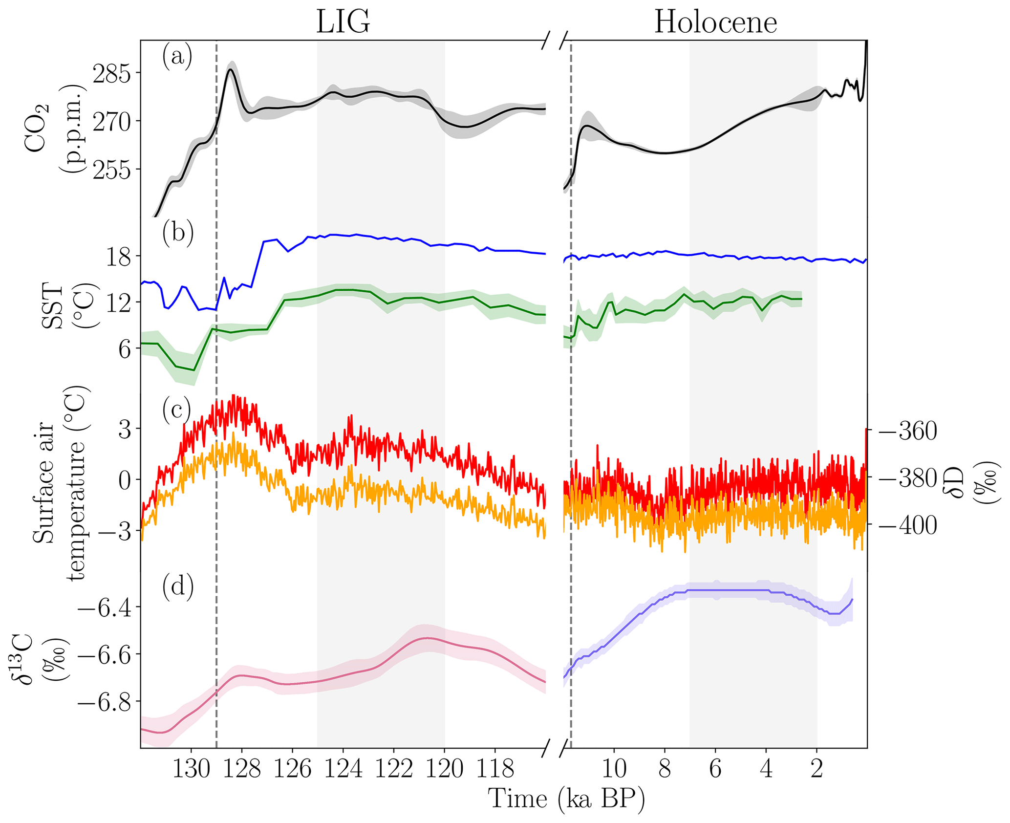
Figure 1LIG and Holocene time series of (a) CO2 stack smoothed with a spline based on the age model AICC2012 (Köhler et al., 2017), (b) sea surface temperatures (SSTs) determined from alkenones and aligned with oxygen isotopes from the Iberian Margin (MD01-2444, blue, Martrat et al., 2007b) and the North Atlantic (GIK23414-6, green, Candy and Alonso-Garcia, 2018), (c) EPICA Dome C ice core (EDC96) deuterium measurements (orange) and estimated surface air temperature anomaly relative to the mean of the last 1 kyr (red, Bazin et al., 2013; Jouzel et al., 2007) on the AICC2012 timescale, and (d) spline of atmospheric δ13C from EPICA Dome C and the Talos Dome ice cores (Holocene, Eggleston et al., 2016) and Monte Carlo average of three Antarctic ice cores atmospheric δ13C (LIG, Schneider et al., 2013) both based on the age model AICC2012. Shading around the lines indicates 1σ. Vertical grey shading indicates the periods of analysis in this paper. Vertical dotted grey lines indicate the commencement of the LIG and Holocene.
Strong polar warming is supported by terrestrial and marine temperature reconstructions. A global analysis of sea surface temperature (SST) records suggests that the mean surface ocean was 0.5 ± 0.3 ∘C warmer during the LIG compared to 1870–1889 (Hoffman et al., 2017), similar to another global estimate, which suggests SSTs were 0.7 ± 0.6 ∘C higher during the LIG compared to the late Holocene (McKay et al., 2011). However, there were differences in the timing of these SST peaks in different regions compared to the 1870–1889 mean: North Atlantic SSTs peaked at +0.6 ± 0.5 ∘C at 125 ka BP (e.g. Fig. 1b) and Southern Hemisphere extratropical SSTs peaked at +1.1 ± 0.5 ∘C at 129 ka BP (Hoffman et al., 2017). On land, proxy records from mid-latitudes to high latitudes indicate higher temperatures during the LIG compared to PI, particularly in North America (Anderson et al., 2014; Axford et al., 2011; Montero-Serrano et al., 2011). Similarly, the EPICA DOME C record suggests that the highest Antarctic temperatures from the last 800 kyr occurred during the LIG (Masson-Delmotte et al., 2010) (Fig. 1c).
Polar warming was also associated with significant changes in vegetation. Pollen records suggest a contraction of tundra and an expansion of boreal forests across the Arctic (CAPE, 2006), in Russia (Tarasov et al., 2005), and in North America (Govin et al., 2015; Muhs et al., 2001; de Vernal and Hillaire-Marcel, 2008). The few Saharan records suggest a green Sahara period during the LIG (Drake et al., 2011; Larrasoaña et al., 2013), consistent with a stronger West African monsoon (Otto-Bliesner et al., 2021). Although these reconstructions indicate changes in vegetation distribution during the LIG, the total amount of carbon stored on land remains poorly constrained.
Recent numerical experiments of the LIG as part of the Paleomodel Intercomparison Project Phase 4 (PMIP4) simulate significant warming over Alaska and Siberia in boreal summer, with mean annual temperature anomalies of close to zero, which is in good agreement with the proxy record (Otto-Bliesner et al., 2021). Despite this and other recent data compilations and modelling efforts (including Bakker et al., 2013), there are many open questions remaining about the LIG. In particular, stronger constraints are needed on the extent of Greenland and Antarctic ice sheets; on ocean circulation and the global carbon cycle, including CaCO3 accumulation in shallow waters; and peat and permafrost carbon storage (Brovkin et al., 2016).
It is important to constrain the state of the Atlantic Meridional Overturning Circulation (AMOC) at the LIG given its significant role in modulating climate. Seven coupled climate models integrated with transient 130–115 ka BP boundary conditions simulate different AMOC trends, with some models producing a strengthening of the AMOC, while others simulate a weakening during the LIG (Bakker et al., 2013). Paleoproxy records suggest equally strong and deep North Atlantic Deep Water (NADW) during the LIG and the Holocene (e.g. Böhm et al., 2015; Lototskaya and Ganssen, 1999), with a possible southward expansion of the Arctic front related to changes in the strength of the subpolar gyre (Mokeddem et al., 2014), and AMOC weakening during a few multi centennial-scale events between 127 and 115 ka BP (e.g. Galaasen et al., 2014b; Helmens et al., 2015; Lehman et al., 2002; Mokeddem et al., 2014; Oppo et al., 2006; Rowe et al., 2019; Tzedakis et al., 2018).
Stable carbon isotopes are a powerful tool for investigating ocean circulation (e.g. Curry and Oppo, 2005; Eide et al., 2017) and the global carbon cycle (e.g. Menviel et al., 2017; Peterson et al., 2014). Since the largest carbon isotope fractionation occurs during photosynthesis, organic matter is enriched in 12C (low δ13C), while atmospheric CO2 and surface water dissolved inorganic carbon (DIC) become enriched in 13C (high δ13C). Organic matter on land includes the terrestrial biosphere, as well as carbon stored in soils, such as in peats and permafrost. Different photosynthetic pathways (which differentiate C3 and C4 plants) fractionate carbon differently, producing typical signatures of about −37 ‰ to −20 ‰ for C3 plants (Kohn, 2010) and around −13 ‰ for C4 plants (Basu et al., 2015), though these values vary with a number of factors, including precipitation, atmospheric CO2 concentration and δ13C, light, nutrient availability, and plant species (Cernusak et al., 2013; Diefendorf et al., 2010; Diefendorf and Freimuth, 2017; Farquhar, 1983; Farquhar et al., 1989; Keller et al., 2017; Leavitt, 1992; Schubert and Jahren, 2012). In the ocean, phytoplankton using the C3 photosynthetic pathway are found to have fractionation during photosynthesis that depends on the concentration of dissolved CO2. Thus, atmospheric δ13CO2 during the LIG (Fig. 1d) is influenced by the cycling of organic carbon within the ocean, changes in the amount of carbon stored in vegetation and soils, temperature-dependent air–sea flux fractionation (Lynch-Stieglitz et al., 1995; Zhang et al., 1995), and on longer timescales by interactions with the lithosphere (Tschumi et al., 2011). The mean surface DIC is enriched by ∼ 8.5 ‰ compared to the atmosphere due to fractionation during air–sea gas exchange (Menviel et al., 2015; Schmittner et al., 2013).
NADW is characterised by low nutrients and high δ13C as a result of a high nutrient and carbon utilisation by marine biota and fractionation during air–sea gas exchange in the northern North Atlantic. Along its path through the Atlantic basin interior, organic matter remineralisation and mixing with southern source waters lowers δ13C, with δ13C values of ∼ 0.5 ‰ in the deep Southern Ocean.
The tight relationship between the water masses' apparent oxygen utilisation, nutrient content and δ13C allows δ13C to be used as a water mass ventilation tracer (e.g. Boyle and Keigwin, 1987; Curry and Oppo, 2005; Duplessy et al., 1988; Eide et al., 2017). The δ13C of benthic foraminifera shells, particularly of the species Cibicides wuellerstorfi, has been found to reliably represent the δ13C signature of DIC (Belanger et al., 1981; Duplessy et al., 1984; Zahn et al., 1986) and has therefore been used to better constrain the extent of different water masses. Mass balances of δ13C between the atmosphere, ocean, and land have been previously used to constrain changes in terrestrial carbon between the last glacial maximum (∼ 20 ka BP) and Holocene (e.g. Peterson et al., 2014). However, on longer timescales, exchanges with the lithosphere including volcanic outgassing (Hasenclever et al., 2017; Huybers and Langmuir, 2009), CaCO3 burial in sediments and weathering, release of carbon from methane clathrates, and the net burial of organic carbon also influence the global mean δ13C. It has been estimated that the amount of carbon both entering and exiting the lithosphere due to weathering and burial of organic carbon fluxes could be from 0.274 to 0.344 Gt C yr−1 (Schneider et al., 2013), though these vary through time (Hoogakker et al., 2006). Over timescales greater than 10 kyr, the influence of weathering and burial of carbon might dominate the δ13C signal (Jeltsch-Thömmes et al., 2019; Jeltsch-Thömmes and Joos, 2020), and thus a mass balance cannot be accurately applied to evaluate terrestrial carbon changes between the LIG and Holocene.
Here, we present a new compilation of benthic δ13C from Cibicides wuellerstorfi spanning the 130–118 ka BP time period. We use this data to compare the δ13C signal of the LIG with that of the Holocene and to determine the difference in average ocean δ13C between the two time periods. We then investigate the AMOC during the LIG with our new benthic δ13C database. Finally, we qualitatively explore the role of the various processes affecting the δ13C difference between the LIG and the Holocene.
2.1 Database
We present a new compilation of benthic δ13C covering the periods 130–118 and 8–2 ka BP. From these two sets of data, we select data pertaining to the LIG and compare it to data from the Holocene. Our database only includes measurements on Cibicides wuellerstorfi as no significant fractionation between the calcite shells and the surrounding DIC has been measured in this species (Belanger et al., 1981; Duplessy et al., 1984; Zahn et al., 1986).
Chen et al. (1995)Cortijo (2003)Members (2006)McIntyre et al. (1999)Schmiedl and Mackensen (2006)Chapman and Shackleton (1999)Holbourn et al. (2005)Hodell et al. (2008)Lyle et al. (2002)McManus et al. (1999)Oppo et al. (1998)Shackleton et al. (1990)Jansen et al. (1996)Shackleton et al. (1990)Curry and Oppo (1997)Duplessy et al. (1984)Bickert and Mackensen (2003)Lyle et al. (2002)Pisias and Mix (1997)Deaney et al. (2017)Zhang et al. (2007)Waelbroeck et al. (2001)Wang et al. (1999)Jullien et al. (2006)Labeyrie et al. (1995)Lee et al. (1999)Wei et al. (2006)Hodell and Channell (2016)Cheng et al. (2004)Ruddiman and Members (1982)Duplessy et al. (1984)Galaasen et al. (2014a)Duplessy et al. (1984)Bickert et al. (1997)Mackensen et al. (2001)Curry et al. (1995)Hodell et al. (2001)Bickert et al. (1997)McCorkle and Holder (2001)Oppo and Fairbanks (1987)Russon et al. (2009)Curry and Oppo (2005)Mix et al. (1991)Bickert and Mackensen (2003)Shackleton et al. (1995)Mix et al. (1991)Schmiedl and Mackensen (1997)Zahn et al. (1986)Sarnthein et al. (1994)Shackleton (1977)Zahn et al. (1986)Bickert and Mackensen (2003)Sarnthein et al. (1994)Shackleton (1977)Freudenthal et al. (2002)Sarnthein et al. (1994)Sarnthein et al. (1994)Duplessy (1996)Sarnthein et al. (1994)Sarnthein et al. (1994)Chapman and Shackleton (1999)Sarnthein (2003)Sarnthein et al. (1994)Sarnthein et al. (1994)Sarnthein et al. (1994)Bickert and Mackensen (2003)Curry et al. (1988)Sarnthein et al. (1994)Lynch-Stieglitz et al. (2006)Sarnthein et al. (1994)Rau et al. (2002)Ruddiman and Members (1982)Vidal et al. (1999)Raymo et al. (2004)Ruddiman and Members (1982)Oppo and Lehman (1995)Raymo et al. (1997)Table 1List of cores for the last interglacial period (LIG). Provided is the core name (“Core”), latitude (“Lat”, ∘), longitude (“Long”, ∘), depth (“Dep”, m), the region, and the reference. Regions are abbreviated as follows: NEA: northeastern Atlantic; NWA: northwestern Atlantic; SWA: southwestern Atlantic; SEA: southeastern Atlantic; SA: southern Atlantic; NP: northern Pacific; SP: southern Pacific; I: Indian. Reference abbreviations are as follows: BW96: Bickert and Wefer (1996); CL82: Curry and Lohmann (1982); dA03: de Abreu et al. (2003); KJ8994: Keigwin and Jones (1989, 1994); KS02: Keigwin and Schlegel (2002); L99: Labeyrie et al. (1999); MB99: Mackensen and Bickert (1999); OH00: Oppo and Horowitz (2000); SH84: Shackleton and Hall (1984); SS0405: Skinner and Shackleton (2004, 2005); VH02: Venz and Hodell (2002); V99: Venz et al. (1999); ZM1011: Zarriess and Mackensen (2010, 2011).

Table 2List of cores for the Holocene. Provided is the core name (“Core”), latitude (“Lat”, ∘), longitude (“Long”, ∘), depth (“Dep”, m) the region, and the reference. Regions are abbreviated as follows: NEA: northeastern Atlantic; NWA: northwestern Atlantic; SWA: southwestern Atlantic; SEA: southeastern Atlantic; SA: southern Atlantic; NP: northern Pacific; SP: southern Pacific; I: Indian. Reference abbreviations are as follows: BW96: Bickert and Wefer (1996); CL82: Curry and Lohmann (1982); dA03: de Abreu et al. (2003); KJ8994 Keigwin and Jones (1989, 1994); KS02: Keigwin and Schlegel (2002); L99: Labeyrie et al. (1999); MB99: Mackensen and Bickert (1999); OH00: Oppo and Horowitz (2000); SH84: Shackleton and Hall (1984); SS0405: Skinner and Shackleton (2004, 2005); VH02: Venz and Hodell (2002); V99: Venz et al. (1999); ZM1011: Zarriess and Mackensen (2010, 2011).
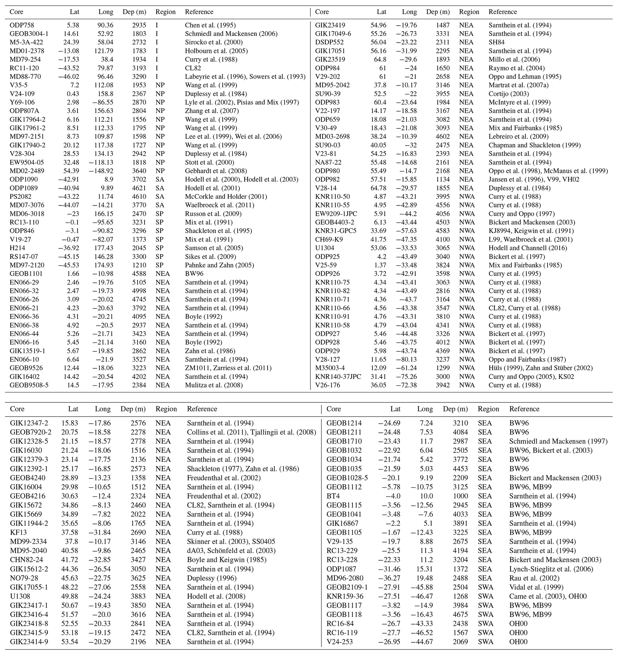
Our compilation is predominantly based on Lisiecki and Stern (2016) (53 cores) but includes 14 cores described in Oliver et al. (2010), as well as a few other records (CH69-K09, Labeyrie et al., 2017; MD03-2664, Galaasen et al., 2014a; MD95-2042, Martrat et al., 2007a; ODP 1063, Deaney et al., 2017; and U1304, Hodell and Channell, 2016). The full core lists are provided in Tables 1 and 2 for the LIG and the Holocene, respectively.
2.2 Age models
Due to the lack of absolute age markers, such as tephra layers, the LIG age models mostly rely on alignment strategies that tie each record to a well-dated reference record. The age model tie points used in this study are taken from the original age model publications. The reference records (LS16; Lisiecki and Stern, 2016) consist of eight regional stacks (one for the intermediate and one for the deep ocean each for the North Atlantic, South Atlantic, Pacific, and Indian oceans) of benthic δ18O that were dated through alignment with other climatic archives such as ice-rafted debris records, synthetic ice core records, and speleothems. The use of regional stacks, rather than a single global stack, improved stratigraphic alignment targets and provided more robust age models. The estimated age model uncertainty (2σ) for this group of cores is 2 kyr. Please refer to Lisiecki and Stern (2016) for further details. Oliver et al. (2010) defined their age tie points assuming that sea level minima and benthic δ18O maxima are synchronous. The benthic δ18O records were aligned with each other and then tied to the Dome Fuji chronology (based on ) (Kawamura et al., 2007). Please refer to Shackleton et al. (2000) and Oliver et al. (2010) for an extensive method description. The age model uncertainty on this group of cores is estimated to range from 1 to 2.5 kyr.
The published age models for the additional cores were determined using similar alignment techniques: SSTs were correlated to the NGRIP Greenland ice core for CH69-K09 and MD95-2042 (Govin et al., 2012). The age model for MD03-2664 was determined by correlating MD03-2664 δ18O with previously dated MD95-2042 δ18O (Galaasen et al., 2014b). ODP 1063 and U1304 δ18O were originally aligned to the LR04 stack (Lisiecki and Raymo, 2005). In order to align all of the records, adjustments to the age models of cores from Oliver et al. (2010) and the five additional cores (CH69-K09, MD95-2042, MD03-2664, ODP 1063, and U1304) were made by aligning the δ18O minima during the LIG to the corresponding δ18O minima of the nearest LS16 stack. The δ18O data before and after the alignment is given in Fig. S1 in the Supplement.
The Holocene age models are based on planktonic foraminifera radiocarbon dates (Stern and Lisiecki, 2014; Waelbroeck et al., 2001) that have been converted into calendar ages using IntCal13 and using reservoir ages based on modern observations (Key et al., 2004), which are assumed to have remained fairly stable across the Holocene. The age uncertainty associated with these Holocene radiocarbon-based age models is generally less than 0.5 kyr. However, it is important to note that Holocene age models from Oliver et al. (2010) were derived using the same method as their LIG age models, leading to larger age uncertainties of about 1–2.5 kyr for this set of Holocene records (four cores). The tie points were used to derive a full age–depth model assuming a constant sedimentation rate between tie points (i.e. linear interpolation).
2.3 Spatial coverage
The spatial distribution of the database for the Holocene and the LIG is shown in Fig. 2, and the depth distribution in each ocean basin is shown in Fig. 3. There are more data in the Atlantic Ocean (65 LIG, 118 Holocene) than in the Pacific (15 LIG, 19 Holocene) and Indian (3 LIG, 7 Holocene) oceans. We used this database to determine (1) if there is a significant difference in the average ocean δ13C signal at the LIG compared to the Holocene and (2) if ocean circulation patterns were comparable. Due to the sparsity of data in the Indian and Pacific oceans, our investigation is primarily focused on the Atlantic. Additionally, the temporal uncertainties (∼ 2 kyr) do not permit an investigation of centennial-scale events, and therefore we restrict our analysis to mean LIG and Holocene conditions.
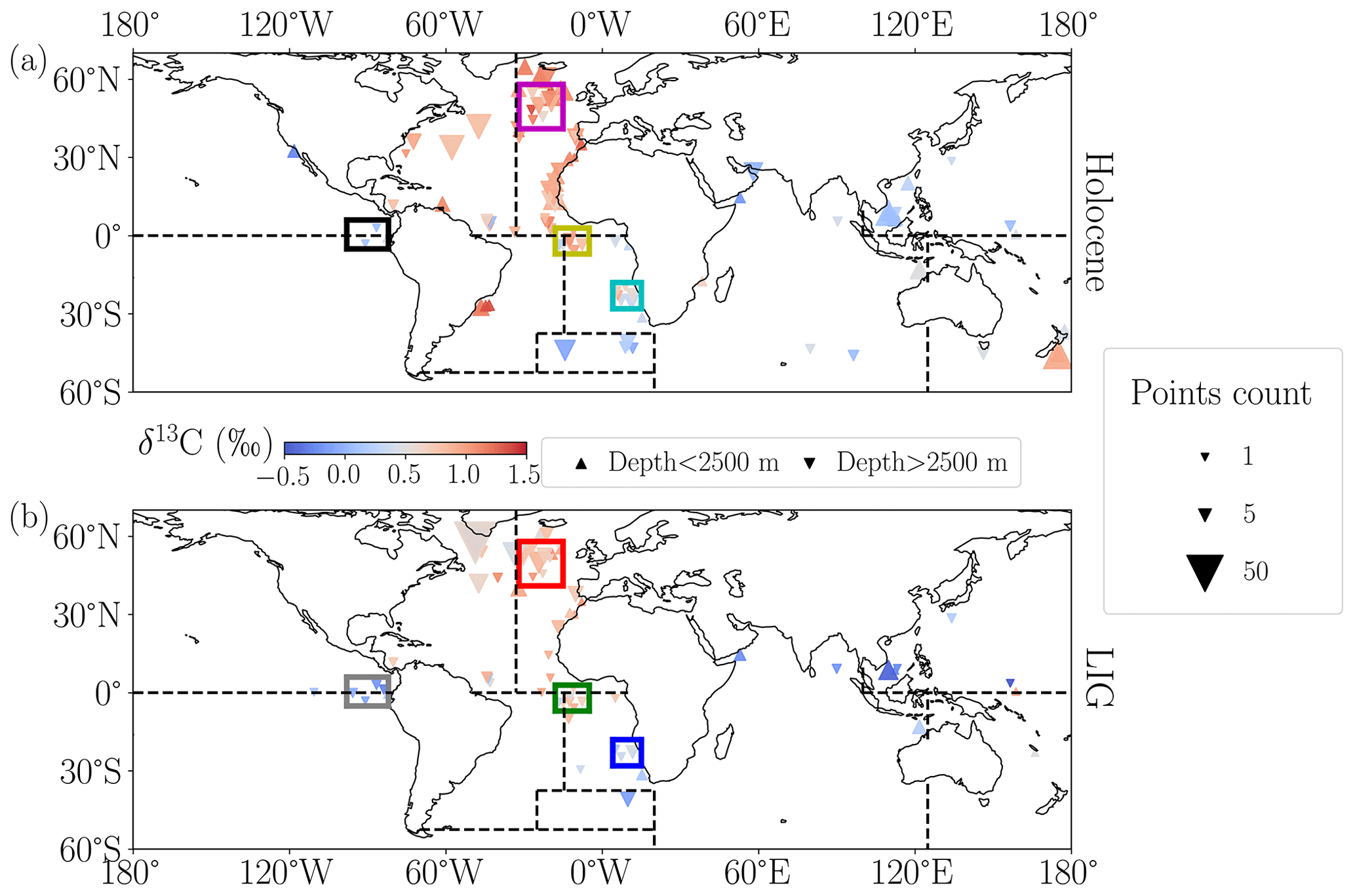
Figure 2Global distribution of benthic foraminifera δ13C covering the periods studied here: the Holocene (7–2 ka BP) (a) and LIG (125–120 ka BP) (b). Symbol size indicates the number of values per core, colour indicates average δ13C, and the triangle direction indicates the proxy depth (upward-pointing triangle: between 1000 and 2500 m depth; downward-pointing triangle: deeper than 2500 m). Four specific regions used in Sect. 3.1 are outlined: eastern equatorial Pacific (black, grey), equatorial Atlantic (yellow, green), southeastern Atlantic (cyan, blue), and northeastern Atlantic (magenta, red). Regional boundaries used to calculate the global volume-weighted mean δ13C (Sect. 3.2) are indicated by dotted black lines as defined in Peterson et al. (2014).
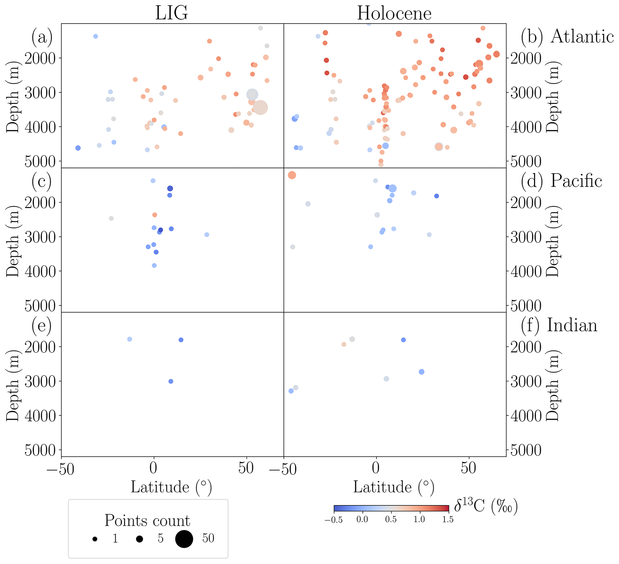
Figure 3Zonal distribution of benthic foraminifera δ13C (‰) during the LIG (125–120 ka BP; a, c, e) and the Holocene (7–2 ka BP; b, d, f) in the Atlantic Ocean (a, b), Pacific Ocean (c, d), and Indian Ocean (e, f). Symbol size indicates the number of measurements per core and colour indicates average δ13C.
The δ13C signal varies significantly regionally and with depth. The highest average δ13C values are associated with NADW and are generally found at depths between ∼ 1500 and 3000 m in the North Atlantic, with organic matter remineralisation and mixing with southern source waters leading to a δ13C decrease along the NADW path. The lowest δ13C values are in the deep South Atlantic (>4000 m) because the Antarctic Bottom Water (AABW) end member is much lower than its NADW counterpart. Since the Indian and Pacific oceans are mostly ventilated from southern-sourced water masses, δ13C generally decreases northward in these two basins.
Since the number of cores is not consistent across the two time periods and given the high regional variability observed in δ13C, it is not possible to simply average all available data to determine the global mean δ13C. Furthermore, the spatial heterogeneity of the data density adds to the complexity of the problem. To address these points, we first analyse differences between the LIG and Holocene records for pre-defined small regions with high data density. We then calculate regional volume-weighted δ13C means for larger regions from which we estimate the global LIG–Holocene anomaly.
3.1 Regional reconstruction of δ13C
We define regions with high densities of cores to reconstruct regional mean δ13C (Fig. 2). These regions need to be small enough to assume reasonably small spatial variability in the δ13C signal and yet still have enough data to establish a reliable statistical difference between the two time periods.
Table 3Regional summary of δ13C below 2500 m depth for the LIG (125–120 ka BP) and Holocene (7–2 ka BP) using a single value per core for each time slice. Shown are the non-volume-weighted means (δ13C, ‰), standard deviations (σ, ‰), and counts (N) for both time periods, along with the time period regional anomalies (Δδ13C, ‰), propagated standard deviations for the anomaly (σ, ‰), and p values from two-sample t tests between the two time periods.

Based on these requirements, four regions are selected: the northeastern Atlantic, the equatorial Atlantic, a region off the Namibian Coast (southeastern Atlantic), and a region around the Galapagos Islands (eastern equatorial Pacific). The boundaries of each region are defined in Table 3.
We then define the time periods within the LIG and the Holocene to perform our analyses. For the Holocene, as most of the available data are dated prior to 2 ka BP, we define the end of our Holocene time period as 2 ka BP. To capture as much of the Holocene data as possible, we include data back to 7 ka BP, ensuring that we do not include instability associated with the 8.2 ka BP event (Alley and Ágústsdóttir, 2005; Thomas et al., 2007). This provides a time span of 5 kyr of data that we will consider for our analysis of the Holocene.
For the LIG, we seek to avoid data associated with the end of the penultimate deglaciation, which is characterised by a benthic δ13C increase in the Atlantic until ∼ 128 ka BP (Govin et al., 2015; Menviel et al., 2019; Oliver et al., 2010, Fig. 4). In addition, a millennial-scale event has been identified in the North Atlantic between ∼ 127 and 126 ka BP (Galaasen et al., 2014b; Tzedakis et al., 2018). Considering the typical dating uncertainties associated with the LIG data (2 kyr), we thus decide to start our LIG time period at 125 ka BP. To ensure that the two time periods are of the same length (5 kyr), we define the LIG period for our analysis to be 125–120 ka BP. We note that our definition should also avoid data associated with the glacial inception (Govin et al., 2015; Past Interglacials Working Group of PAGES, 2016). We verify that the LIG time period has sufficient data across the selected four regions, noting that the highest density of data falls within the 125–120 ka BP time period – particularly in the equatorial Atlantic and southeastern Atlantic (Fig. 4b, c).

Figure 4Benthic foraminifera δ13C (left y axis, ‰) during the LIG (left) and Holocene (right) for four defined regions: northeastern Atlantic (a), equatorial Atlantic (b), southeastern Atlantic (c), and eastern equatorial Pacific (d). Data are presented in discrete time slices spanning 1 kyr. Only cores deeper than 2500 m are shown. Circular, coloured points connected by lines show each average δ13C value per core per time slice. Black symbols represent δ13C averages per slice. Each slice has a corresponding averaged depth (right y axis, m), with 1 standard deviation on either side shown on the bars. Slices with an average depth within ±300 m of the mean core depth of all slices are represented with a square point. Slices with an average depth 300 m shallower than the mean are shown with an upward triangle, and slices that are than 300 m deeper than the mean are shown with a downward triangle. Shading shows 1 standard deviation on either side of the mean for slices where more than one point exists.
We round the data to the nearest 1 kyr, find an average per 1 kyr, and refer to this as a time slice. We consider the LIG–Holocene anomaly across these two time periods for the four regions selected, and qualitatively consider the influence of changes in the average depth in which the proxies were recorded, as indicated by the direction of the black triangles in Fig. 4.
The average δ13C anomaly between the LIG and Holocene periods for cores deeper than 2500 m is consistent across the different regions despite their geographic separation, suggesting a significantly lower δ13C during the LIG than the Holocene, with differences ranging from −0.13 ‰ in the northeastern Atlantic to −0.20 ‰ in the equatorial Pacific (Table 3). The statistical significance between the two time periods is established using a two-tailed t test on data of one mean value per core and spans all time slices (125–120 and 7–2 ka BP). The t test shows that there is a statistically significant difference everywhere except in the equatorial Atlantic, with confidence intervals varying from 0.13 in the equatorial Atlantic to 0.04 in the northeastern Atlantic. When using a single tail t test instead, the difference becomes significant in the equatorial Atlantic, giving a new p value of 0.02. Figure 4 suggests that the difficulty in determining significance in this region for cores deeper than 2500 m might be due to a singular outlier measurement in the equatorial Atlantic: a value of −0.23 ‰ from GeoB1118 at ∼ 3.5 ka BP. If this value is excluded, then an anomaly of −0.22 with a p value less than 0.005 is observed.
We also compare the distribution of δ13C for cores deeper than 2500 m for three overlapping periods within the LIG (early LIG: 128–123 ka BP; LIG: 125–120 ka BP; late LIG: 123–118 ka BP). The results for the four regions are shown in Fig. 5. The statistical characteristics do not show much variation between the LIG and late LIG δ13C distributions. In the equatorial Pacific, the difference between the early LIG and the Holocene is smaller than between the LIG and Holocene, but this is countered with a larger difference in the equatorial Atlantic between the early LIG and Holocene. The spread in the data is generally larger during the Holocene than during the other time periods, which might be due to the greater number of measurements during the Holocene. The spread of data during the early LIG is slightly larger than during the LIG and late LIG in the equatorial and southeastern Atlantic. The equatorial Atlantic is the only region that displays significantly more points with lower δ13C during the early LIG. Overall, these distributions do not suggest that the LIG–Holocene anomalies that we have determined would be significantly impacted by slight variations in the selected time window. We perform an analysis of variance (ANOVA) on each region and post hoc tests on the data. We find that the Holocene data are significantly different from the three LIG periods in the northeastern Atlantic, the southeastern Atlantic, and the equatorial Pacific, while the three periods within the LIG are not significantly different from each other for any of the regions.
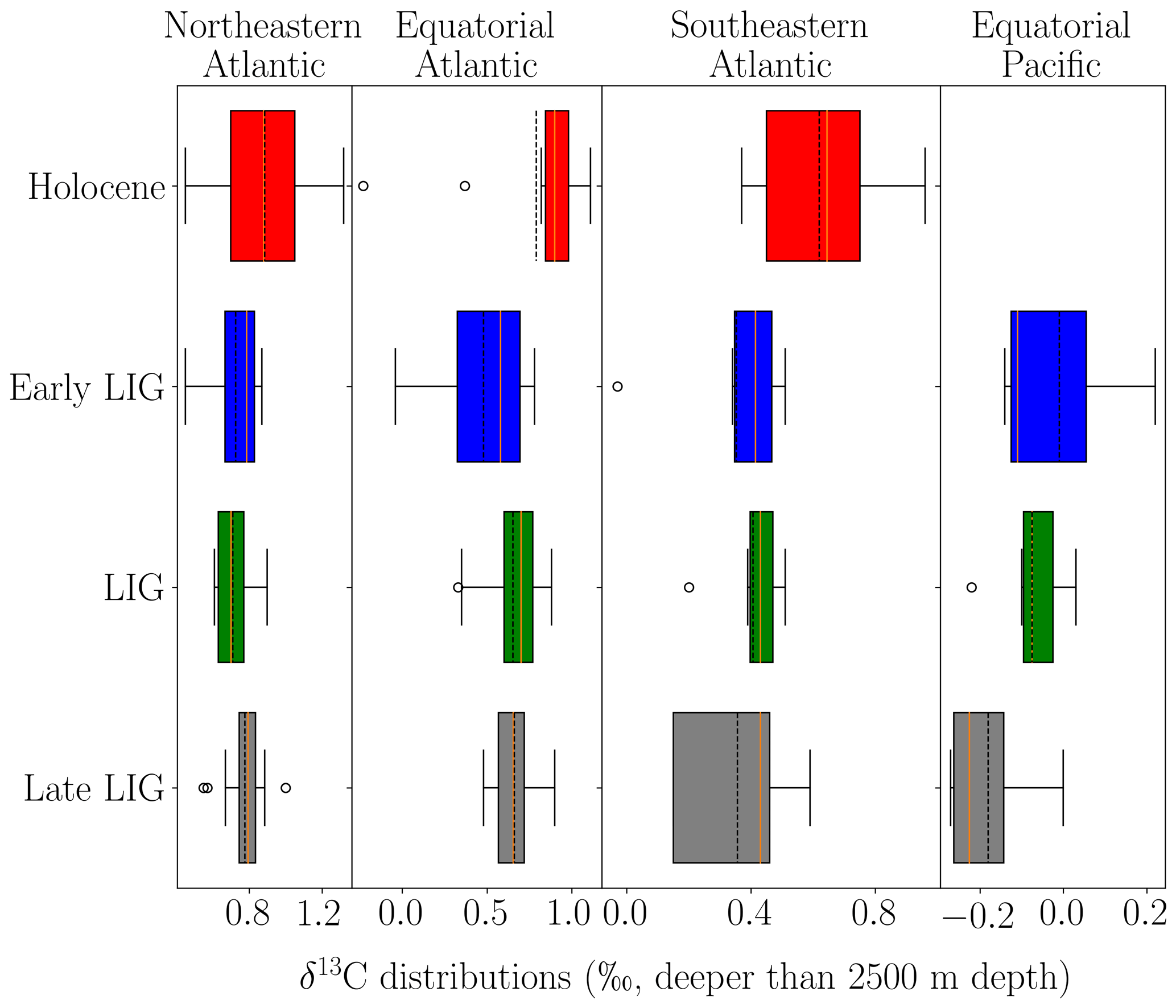
Figure 5Distributions of δ13C for all core measurements deeper than 2500 m during the Holocene (7–2 ka BP, red), the early LIG (128–123 ka BP), the LIG (125–120 ka BP), and the late LIG (123–118 ka BP) across four regions (equatorial Pacific, equatorial Atlantic, southeastern Atlantic, northeastern Atlantic). The lower end of the box indicates quartile 1 (Q1), and the upper end indicates quartile 3 (Q3). Orange vertical lines show the median, and dotted vertical lines show the mean. The whiskers indicate the lower and upper fences of the data calculated as Q1 − 1.5 × (Q3 − Q1) and Q3 + 1.5 × (Q3 − Q1), respectively, and the clear circles are outliers.
3.2 Volume-weighted regional δ13C
The second approach we use to further constrain the LIG–Holocene δ13C anomaly is to estimate the volume-weighted regional δ13C. We define our regional boundaries based on the regions described in Peterson et al. (2014); however, we only include the regions where there are enough data to justify an analysis. For all the data in each of these regions, we calculate a mean value by taking the direct averages of all data. We divide the ocean basins into eight regions (Table 4, shown in Fig. 2) and calculate the volume-weighted averages δ13C for each of these regions. Since the Atlantic and Pacific oceans have more data than the Indian Ocean, there is greater confidence in the δ13C estimates for these regions. These regional averages are then used to calculate a global volume-weighted δ13C.
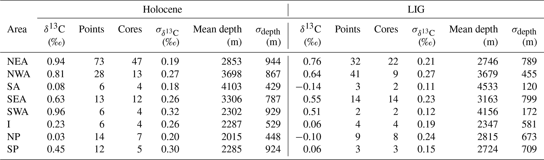
Table 4Regional breakdown of δ13C data for all depths during the Holocene (7–2 ka BP) and LIG (125–120 ka BP) averaged across the 1 kyr time slices. For each region: the average number of data points (labelled as “Points”) and cores per time slice (labelled as “Cores”), the average standard deviation of δ13C per time slice (‰), the mean depth (m) across time slices, and the standard deviation of depth (m) between time slices (σdepth). Regions are abbreviated as follows: NEA: northeastern Atlantic; NWA: northwestern Atlantic; SA: southern Atlantic; SEA: southeastern Atlantic; SWA: southwestern Atlantic; I: Indian, NP: northern Pacific; SP: southern Pacific.
Results for the Atlantic and Pacific oceans are given in Fig. 6 and show a mean LIG–Holocene anomaly of −0.21 ‰ and −0.27 ‰, respectively, slightly higher than the range of estimates for the four regions selected in Sect. 3.1. There is a higher offset estimated in this definition of the southwestern Atlantic (−0.45 ‰) than in Sect. 3.1; however, there are only four cores available in this region during the Holocene and two during the LIG.
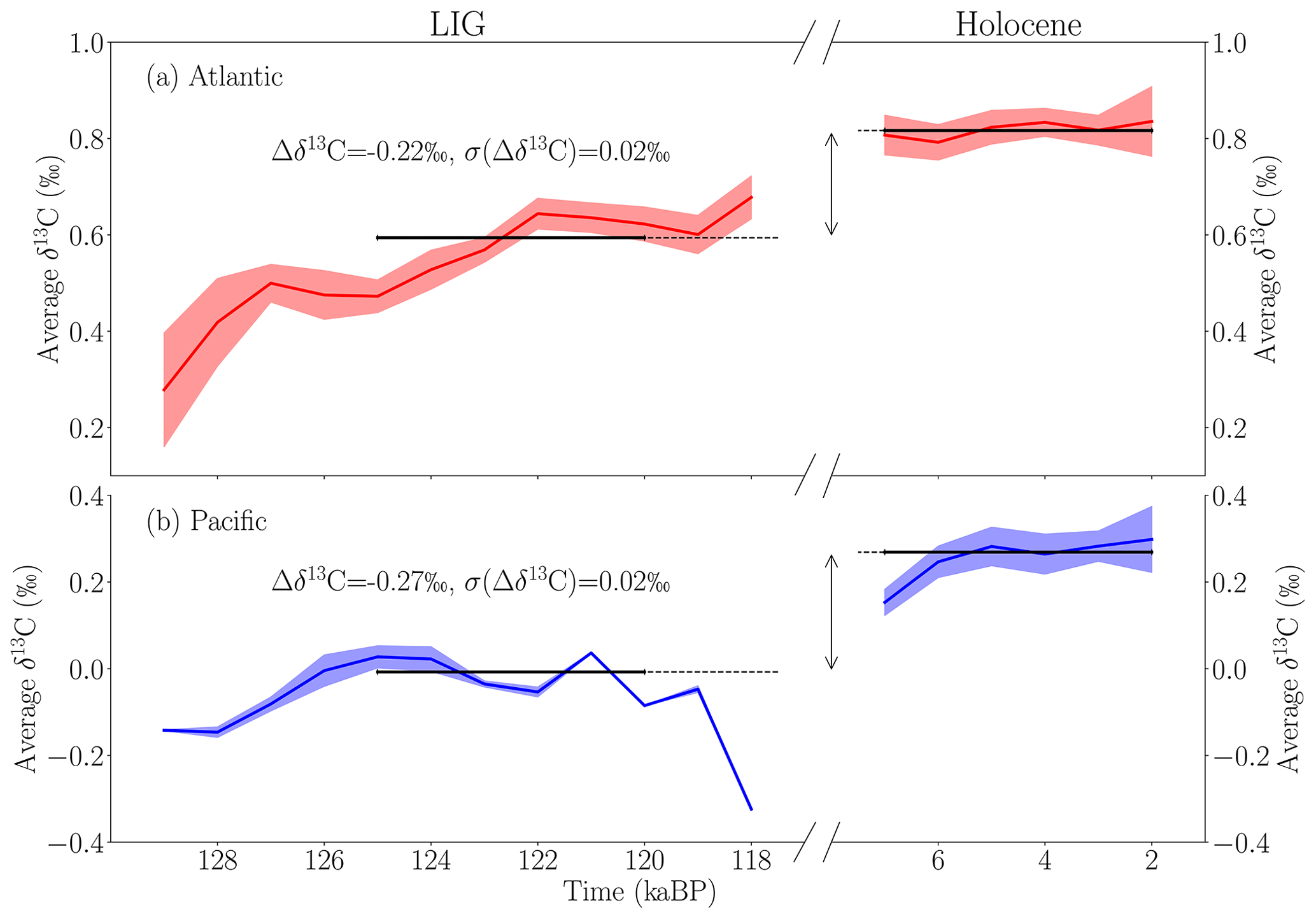
Figure 6Comparison of volume-weighted δ13C for the Atlantic (red) and Pacific (blue) for the LIG and Holocene, calculated using the regions from Peterson et al. (2014) from data covering all depths. Solid coloured lines indicate the mean volume-weighted δ13C, and the shading indicates the volume-weighted sum of square deviations from the mean. The horizontal bars indicate the mean of the stable period determined from the regional analysis as defined in Sect. 3.1 (LIG: 125–120 ka BP; Holocene: 7–2 ka BP), with the Δδ13C indicating the mean anomaly between these two averages and the standard deviation (σ(δ13C), ‰).
The estimated LIG–Holocene anomaly in the southern Pacific is relatively high at −0.39 ‰, giving a relatively large Pacific anomaly estimate of −0.27 ‰. This could be due in part to the deeper location of the LIG cores compared to the mean of the Holocene cores (439 m difference, Table 4). There is less confidence in the estimate of the Pacific volume-weighted mean since the proxy data are sparse, and the majority of cores are from the eastern equatorial Pacific as shown in Fig. 2. We also note that the average depths of cores from the Pacific Ocean (LIG: 2711 m; Holocene: 2131 m) and Indian Ocean (LIG: 2383 m; Holocene: 2303 m) are shallower than that of the Atlantic Ocean (LIG: 3531 m; Holocene: 3157 m; Fig. 3). However, as the vertical gradient below 2000 m depth in the Pacific Ocean is small (e.g. Eide et al., 2017), this might not significantly impact our results.
There is a small positive trend in the average Atlantic δ13C from 125 ka BP, reaching a maximum value at 118 ka BP (Fig. 6). The average core depth over the 125–120 ka BP time period does not suggest that a change in the mean depth could explain this variation. Fitting a linear regression over this period indicates an increase in δ13C of 0.03 ‰ kyr−1 in the Atlantic, with a p value of 0.01 and an R2 of 0.85 (Fig. 4a). For the Pacific, there is a ∼ 0.13 ‰ increase in δ13C between 7 and 5 ka BP, which could be associated with the early Holocene terrestrial regrowth (Menviel and Joos, 2012).
For the Indian Ocean, we only include four cores, as these are the only ones spanning both the LIG and Holocene. An LIG anomaly of −0.13 ‰ in the Indian Ocean compared to the Holocene is therefore associated with higher uncertainties. The whole ocean mean LIG δ13C anomaly is −0.25 ‰, but it is associated with higher uncertainties than each region anomaly.
Both the regional analysis of our new database and our volume-weighted estimate indicate that the global mean δ13C was about 0.2 ‰ lower during the LIG than during the Holocene. We further test the robustness of this result in the next section.
3.3 Reconstruction of the LIG Atlantic Meridional Overturning Circulation
In this section, we analyse the spatial δ13C distribution in the Atlantic Ocean to assess potential changes in the penetration depth and southward expansion of NADW during the LIG, defined here as 125–120 ka BP, with respect to the Holocene. A change in NADW might influence our estimate of the mean δ13C, given that most of the available data are localised in the Atlantic Ocean.
We use simple statistical regression models to reconstruct NADW and AABW separately with a quadratic-with-depth and linear-with-latitude equation following the method of Bengtson et al. (2019). For consistency, the regression algorithm only includes records from cores that span both the LIG and Holocene and uses a weighted least-squares approach, where the weighting equals the number of samples per core. The modelled region is defined between 40∘ S and 60∘ N as this is the region where we can expect to find both the NADW and AABW δ13C signals.
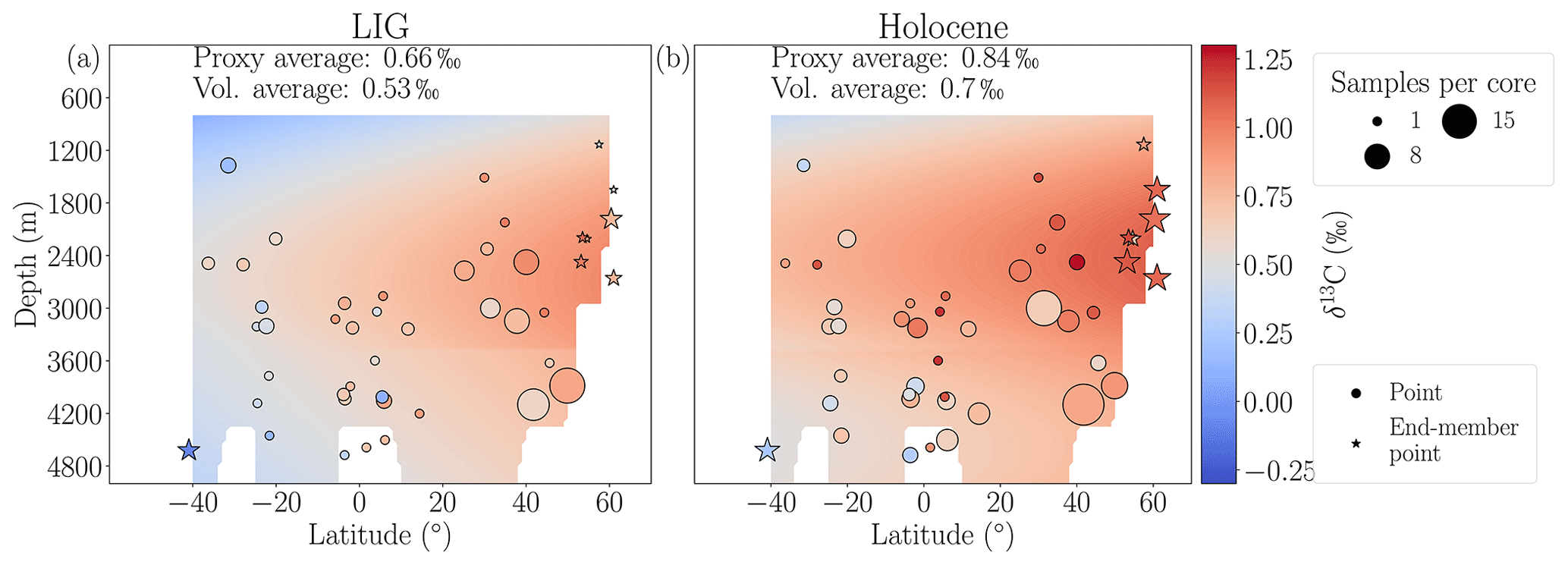
Figure 7Reconstructed Atlantic δ13C (‰) meridional section during the LIG (125–120 ka BP) and Holocene (7–2 ka BP). The circular points represent the proxy data, showing the average δ13C with colour and the number of points per core with size. The stars represent the proxy data that make up the end members. Background shading shows the reconstructed δ13C using a quadratic statistical regression of the proxy data following the method described in Bengtson et al. (2019).
The results are shown in Fig. 7. We test the robustness of our statistical model using the jackknifing technique. We systematically exclude each individual core from the database one at a time, fit the parameters using this modified database, and compare the model prediction against the core, which was excluded. This produces small variations in the average mean response of the statistical models (the standard deviations were 0.01 ‰ for both the LIG and Holocene, respectively).
We calculate end member values based on proxies located near the water mass sources. These are taken as 0.79 ‰ and 1.02 ‰ for NADW for the LIG and Holocene, respectively, and −0.09 ‰ and 0.23 ‰ for AABW for the LIG and Holocene, respectively. The end member values are calculated as the average of cores shallower than 3000 m but deeper than 1000 m and located between 50 and 70∘ N for NADW. The NADW end member cores have an average depth of 2043 m and a standard deviation of 478 m during the LIG. For the AABW end member, the only eligible core is ODP1089, which is at ∼ 41∘ S and 4621 m.
The mean volume-weighted δ13C for the Atlantic Ocean between 40∘ S and 60∘ N based on this interpolation is 0.53 ‰ for the LIG and 0.70 ‰ for the Holocene (Fig. 7). This suggests a 0.17 ‰ lower Atlantic δ13C at the LIG than the Holocene. Our statistical reconstruction points to a very similar NADW depth (∼ 2600 m) for both time periods (Fig. 7). The NADW depth is defined here as the depth of maximum δ13C in the North Atlantic.
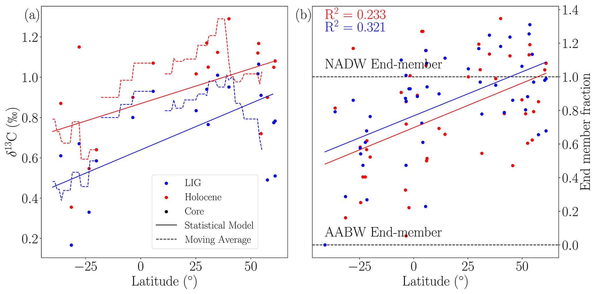
Figure 8The meridional gradient of the Atlantic Ocean benthic δ13C (‰). (a) Holocene (red) and LIG (blue) δ13C for each core (points) between 1000 and 3000 m. Dotted lines are the moving averages of the cores. Solid lines indicate the results of our statistical model at 2000 m. (b) Average δ13C for each record deeper than 1000 m as a proportion of the end members. A value of one indicates the NADW end member, and a value of zero indicates the AABW end member. Solid lines show the linear regressions of the records.
We also investigate the meridional gradient in δ13C in the Atlantic Ocean to determine whether the NADW southward penetration, transport, and remineralisation rates were significantly different during the LIG compared to the Holocene. We only consider cores that are located between depths of 1000 and 3000 m in order to stay within the main pathway of NADW (Fig. 8a). Though there is significant scatter, in accordance with our previous findings, a moving average through the Holocene and the LIG data shows that LIG δ13C is typically lower than the Holocene counterparts. However, the meridional δ13C statistical model gradients are not very different for the LIG (0.0036 ‰ per degree latitude) and the Holocene (0.0030 ‰ per degree latitude) (Fig. 8a), suggesting a similar southward penetration of NADW.
Using δ13C of the end members for NADW and AABW, we use a simple binary mixing model for all cores deeper than 1000 m to estimate changes in NADW penetration (Fig. 8b). The LIG and Holocene δ13C slopes in the Atlantic are similar, indicating similar southward penetration of NADW during both time periods. This suggests that the differences in δ13C between the two time periods is most likely due to change in end member values, while the mean Atlantic oceanic circulation was likely similar.
Based on our analysis, there appears to be no significant difference in the mean time-averaged AMOC between the LIG and the Holocene. Negative LIG–Holocene anomalies are found for each of the smaller regions selected (northeastern Atlantic, equatorial Atlantic, southeastern Atlantic, and eastern equatorial Pacific), with statistical significance seen in all regions except the equatorial Atlantic, where an unusual low δ13C value in one core is responsible for narrowing the difference between the two period means. Additionally, our volume-weighted mean δ13C estimates have similar anomalies in the Atlantic and Pacific oceans (−0.21 ‰ and −0.27 ‰, respectively, Fig. 6).
One of the goals of our study is to assess the mean change in oceanic δ13C between the LIG and the Holocene. Given the uncertainties in the chronologies, avoiding data that pertains to deglaciation, and capturing the same length of time during the LIG and the Holocene, we chose the periods 125 to 120 ka BP for the LIG and 7 to 2 ka BP for the Holocene. Using a similar geographical distribution of data points for both periods, we find that the oceanic δ13C was ∼ 0.2 ‰ lower during the LIG than the Holocene.
Our analysis of the δ13C signal suggests consistent LIG–Holocene δ13C anomalies in different regions of the Atlantic basins, as well as in the Pacific and Indian oceans, even if there are significant uncertainties with the later due to fewer available records. The δ13C distribution in the Atlantic Ocean suggests that there was no significant mean change in the southward penetration or depth of NADW during the LIG (125–120 ka BP) compared to the Holocene (7–2 ka BP). A statistical reconstruction of the early LIG (128–123 ka BP) δ13C compared to our 125–120 ka BP reconstruction does not reveal a significant difference in either the NADW core depth or NADW extent, as indicated by the meridional δ13C gradients (Fig. S2). The volume-weighted average δ13C during the early LIG is 0.06 ‰ lighter than during the LIG period considered here (125–120 ka BP). Since both time slices (128–123 and 125–120 ka BP) are 5 kyr averages and include dating uncertainties of ∼ 2 kyr, it is not possible to resolve potential centennial-scale oceanic circulation changes (e.g. Galaasen et al., 2014b; Tzedakis et al., 2018).
Explanations for the 0.2 ‰ lower δ13C anomaly in the ocean may include a redistribution between the ocean–atmosphere system. Such a redistribution can result from a change in end member values (Fig. 8). As fractionation during air–sea gas exchange is temperature dependent, globally higher SSTs at the LIG could lead to a lower oceanic δ13C. However, the effect of this is likely small (Brovkin et al., 2002) and would also lead to a higher atmospheric δ13CO2 at the LIG, which is inconsistent with Antarctic ice core measurements that suggest an anomaly of −0.3 ‰ (Schneider et al., 2013). Lower nutrient utilisation in the North Atlantic would decrease surface ocean δ13C and thus the δ13C end members. However, this would also imply that less organic carbon would be remineralised at depth. Therefore, it is unlikely that the lower average oceanic mean δ13C results from a change in end members through lower surface ocean nutrient utilisation. Currently, there is still a lack of constraints on nutrient utilisation in these end member regions during the LIG compared to the Holocene. Therefore, the lower δ13C in the ocean–atmosphere system cannot be explained by a simple redistribution of δ13C between the atmosphere and the ocean.
An alternative explanation for the anomaly is a change in the terrestrial carbon storage, which has a typical signature of approximately −37 ‰ to −20 ‰ for C3-derived plant material (Kohn, 2010) and −13 ‰ for C4-derived plant material (Basu et al., 2015). The total land carbon content at the LIG is poorly constrained. Proxies generally suggest extensive vegetation during the LIG compared to the Holocene (CAPE, 2006; Govin et al., 2015; Larrasoaña et al., 2013; Muhs et al., 2001; Tarasov et al., 2005; de Vernal and Hillaire-Marcel, 2008), which would imply a greater land carbon store. However, other terrestrial carbon stores including peatlands and permafrost may also have differed during the LIG compared to the Holocene. With an estimated ∼ 550 Gt C stored in peats today (mean δ13C ∼ −28 ‰; Dioumaeva et al., 2002; Novák et al., 1999) and ∼ 1000 Gt C in the active layer in permafrost, which may have been partially thawed during the LIG (Reyes et al., 2010; Schuur et al., 2015; Stapel et al., 2018), less carbon stored in peat and permafrost at the LIG could have led to a lower total land carbon store compared to the Holocene. However, it is not possible to infer this total land carbon change from the oceanic and atmospheric δ13C anomalies because it cannot be assumed that the mass of carbon and 13C is preserved within the ocean–atmosphere–land biosphere system on glacial–interglacial timescales. There is indeed continuous exchange of carbon and 13C between the lithosphere and the coupled ocean, atmosphere, and land biosphere carbon reservoirs. Isotopic perturbations associated with changes in the terrestrial biosphere are communicated to the burial fluxes of organic carbon and CaCO3 and are therefore attenuated on multi-millennial time scales (Jeltsch-Thömmes et al., 2019; Jeltsch-Thömmes and Joos, 2020). Nevertheless, when hypothetically neglecting any exchange with the lithosphere, we find that the change in terrestrial carbon needed to explain the difference in δ13C would be on the order of 310 ± 44 Gt C less during the LIG than the Holocene (Text S1).
In addition, due to the warmer conditions at the LIG than during the Holocene, there could have been a release of methane clathrates which would have added isotopically light carbon (δ13C: ∼ −47 ‰) to the ocean-atmosphere system. However, available evidence suggests that geological CH4 sources are rather small (Bock et al., 2017; Dyonisius et al., 2020; Hmiel et al., 2020; Saunois et al., 2020) making this explanation unlikely, although we cannot completely exclude the possibility that the geological CH4 source was larger at the LIG than the Holocene. Similarly, since δ13CO2 from volcanic outgassing has a similar value to atmospheric δ13CO2 (Brovkin et al., 2016) and modelling suggests volcanic outgassing likely only had a minor impact on δ13CO2 (Roth and Joos, 2012), it is unlikely that volcanic outgassing of CO2 played a significant role in influencing the mean oceanic δ13C.
While changes in terrestrial carbon could have impacted the oceanic δ13C at the LIG, the LIG–Holocene differences in the isotopic signal of both the atmosphere and ocean were most likely due to a long-term imbalance between the isotopic fluxes to and from the lithosphere, including the net burial (or redissolution) of organic carbon and CaCO3 in deep-sea sediments, and changes in shallow water sedimentation and coral reef formation (Jeltsch-Thömmes and Joos, 2020).
We present a new compilation of benthic δ13C from 130 to 115 ka BP covering the LIG. Over this time period, benthic δ13C generally display a maximum value at ∼ 121 ka BP (±2 kyr), in phase with the maximum atmospheric δ13CO2 (LIG value of −6.5 ‰ at ∼ 120 ka BP). As there are significant chronological uncertainties associated with LIG records, we analyse data between 125 and 120 ka BP to avoid data associated with millennial-scale events and the deglaciation. We compare this LIG benthic δ13C data to a similar database covering the Holocene (7–2 ka BP). We find that during these specific time periods, LIG oceanic δ13C was about 0.2 ‰ lower than during the Holocene. This anomaly is consistent across different regions in the Atlantic Ocean. Even though there are fewer records available, benthic δ13C data from the Pacific Ocean also support an anomaly of about 0.2 ‰.
An analysis of δ13C gradients across the Atlantic Ocean suggests that there were no significant changes in mean long-term ocean circulation between the two intervals. While reduced high northern latitude peat and permafrost caused by higher temperatures at the LIG than during the Holocene (Otto-Bliesner et al., 2021) could have lead to a lower atmospheric and oceanic δ13C, the most likely explanation for the lower LIG oceanic δ13C is a long-term imbalance in the weathering and burial of carbon. Additional studies are required to further constrain the LIG carbon balance.
The data are published on Research Data Australia at DOI https://doi.org/10.26190/5efe841541f3b (Bengtson et al., 2020).
The supplement related to this article is available online at: https://doi.org/10.5194/cp-17-507-2021-supplement.
SAB, LCM, and KJM designed the research. CDP and LEL provided significant portions of the δ13C data. SAB, LCM, KJM, and LM analysed the data and developed the methodology. FJ assisted in the interpretation of the results. SAB prepared the manuscript with contributions from all co-authors.
The authors declare that they have no conflict of interest.
Shannon A. Bengtson acknowledges funding from the Australian Government Research Training Program Scholarship. Laurie C. Menviel and Katrin J. Meissner acknowledge funding from the Australian Research Council. Computational resources were provided by the NCI National Facility at the Australian National University through awards under the Merit Allocation Scheme, the Intersect allocation scheme, and the UNSW HPC at NCI Scheme. Fortunat Joos acknowledges funding from the Swiss National Science Foundation. This study was facilitated by the PAGES QUIGS working group.
This research has been supported by the Australian Research Council (grant nos. FT180100606 and DP180100048) the Swiss National Science Foundation (grant no. 200020_172476), and the Australian Government Research Training Program Scholarship.
This paper was edited by Marit-Solveig Seidenkrantz and reviewed by two anonymous referees.
Alley, R. B. and Ágústsdóttir, A. M.: The 8k event: cause and consequences of a major Holocene abrupt climate change, Quaternary Sci. Rev., 24, 1123–1149, https://doi.org/10.1016/j.quascirev.2004.12.004, 2005. a
Anderson, R. S., Jiménez-Moreno, G., Ager, T., and Porinchu, D. F.: High-elevation paleoenvironmental change during MIS 6–4 in the central Rockies of Colorado as determined from pollen analysis, Quaternary Res., 82, 542–552, https://doi.org/10.1016/j.yqres.2014.03.005, 2014. a
Axford, Y., Briner, J., Francis, D., Miller, G., Walker, I., and Wolfe, A.: Chironomids record terrestrial temperature changes throughout Arctic interglacials of the past 200 000 yr, Geol. Soc. Am. Bull., 123, 1275–1287, https://doi.org/10.1130/B30329.1, 2011. a
Bakker, P., Stone, E. J., Charbit, S., Gröger, M., Krebs-Kanzow, U., Ritz, S. P., Varma, V., Khon, V., Lunt, D. J., Mikolajewicz, U., Prange, M., Renssen, H., Schneider, B., and Schulz, M.: Last interglacial temperature evolution – a model inter-comparison, Clim. Past, 9, 605–619, https://doi.org/10.5194/cp-9-605-2013, 2013. a, b
Basu, S., Agrawal, S., Sanyal, P., Mahato, P., Kumar, S., and Sarkar, A.: Carbon isotopic ratios of modern C3–C4 plants from the Gangetic Plain, India and its implications to paleovegetational reconstruction, Palaeogeogr. Palaeocl., 440, 22–32, https://doi.org/10.1016/j.palaeo.2015.08.012, 2015. a, b
Bazin, L., Landais, A., Lemieux-Dudon, B., Toyé Mahamadou Kele, H., Veres, D., Parrenin, F., Martinerie, P., Ritz, C., Capron, E., Lipenkov, V. Y., Loutre, M.-F., Raynaud, D., Vinther, B. M., Svensson, A. M., Rasmussen, S. O., Severi, M., Blunier, T., Leuenberger, M. C., Fischer, H., Masson-Delmotte, V., Chappellaz, J. A., and Wolff, E. W.: delta Deuterium measured on ice core EDC on AICC2012 chronology, PANGAEA, https://doi.org/10.1594/PANGAEA.824891, 2013. a
Belanger, P. E., Curry, W. B., and Matthews, R. K.: Core-top evaluation of benthic foraminiferal isotopic ratios for paleo-oceanographic interpretations, Palaeogeogr. Palaeocl., 33, 205–220, https://doi.org/10.1016/0031-0182(81)90039-0, 1981. a, b
Bengtson, S. A., Meissner, K. J., Menviel, L., Sisson, S., and Wilkin, J.: Evaluating the extent of North Atlantic Deep Water and the mean Atlantic δ13C from statistical reconstructions, Paleoceanogr. Paleocl., 34, 1022–1036, https://doi.org/10.1029/2019PA003589, 2019. a, b
Bengtson, S. A., Menviel, L., Meissner, K. J., Missiaen, L., Peterson, C., Lisiecki, L., and Joos, F.: Benthic δ13C during the last interglacial and the Holocene, UNSW, Australian Research Data Commons, https://doi.org/10.26190/5efe841541f3b, 2020. a
Bereiter, B., Eggleston, S., Schmitt, J., Nehrbass-Ahles, C., Stocker, T. F., Fischer, H., Kipfstuhl, S., and Chappellaz, J.: Revision of the EPICA Dome C CO2 record from 800 to 600 kyr before present, Geophys. Res. Lett., 42, 542–549, https://doi.org/10.1002/2014GL061957, 2015. a
Bickert, T. and Mackensen, A.: Last Glacial to Holocene Changes in South Atlantic Deep Water Circulation, in: The South Atlantic in the Late Quaternary: Reconstruction of Material Budgets and Current Systems, edited by: Wefer, G., Mulitza, S., and Ratmeyer, V., Springer, Berlin and Heidelberg, Germany, 671–693, https://doi.org/10.1007/978-3-642-18917-3_29, 2003. a, b, c, d, e, f, g
Bickert, T. and Wefer, G.: Late Quaternary Deep Water Circulation in the South Atlantic: Reconstruction from Carbonate Dissolution and Benthic Stable Isotopes, in: The South Atlantic: Present and Past Circulation, edited by: Wefer, G., Berger, W. H., Siedler, G., and Webb, D. J., Springer, Berlin and Heidelberg, Germany, 599–620, https://doi.org/10.1007/978-3-642-80353-6_30, 1996. a, b
Bickert, T., Curry, W. B., and Wefer, G.: Late Pliocene to Holocene (2.6–0 Ma) western equatorial Atlantic deep-water circulation: inferences from benthic stable isotopes, Proc. Ocean Drill. Program Sci. Results, 154, 239–254, 1997. a, b, c, d, e, f
Bickert, T., Wefer, G., and Müller, P. J.: Stable isotopes and sedimentology of core GeoB1032-2, PANGAEA, https://doi.org/10.1594/PANGAEA.103613, 2003. a
Bock, M., Schmitt, J., Beck, J., Seth, B., Chappellaz, J., and Fischer, H.: Glacial/interglacial wetland, biomass burning, and geologic methane emissions constrained by dual stable isotopic CH4 ice core records, P. Natl. Acad. Sci. USA, 114, 5778–5786, https://doi.org/10.1073/pnas.1613883114, 2017. a
Böhm, E., Lippold, J., Gutjahr, M., Frank, M., Blaser, P., Antz, B., Fohlmeister, J., Frank, N., Andersen, M. B., and Deininger, M.: Strong and deep Atlantic meridional overturning circulation during the last glacial cycle, Nature, 517, 73–76, https://doi.org/10.1038/nature14059, 2015. a
Boyle, E. A.: Cadmium and δ13C Paleochemical Ocean Distributions During the Stage 2 Glacial Maximum, Annu. Rev. Earth Pl. Sc., 20, 245–287, https://doi.org/10.1146/annurev.ea.20.050192.001333, 1992. a, b
Boyle, E. A. and Keigwin, L. D.: Comparison of Atlantic and Pacific paleochemical records for the last 215 000 years: changes in deep ocean circulation and chemical inventories, Earth Planet. Sci. Lett., 76, 135–150, https://doi.org/10.1016/0012-821X(85)90154-2, 1985. a
Boyle, E. A. and Keigwin, L.: North Atlantic thermohaline circulation during the past 20 000 years linked to high-latitude surface temperature, Nature, 330, 35–40, https://doi.org/10.1038/330035a0, 1987. a
Brovkin, V., Bendtsen, J., Claussen, M., Ganopolski, A., Kubatzki, C., Petoukhov, V., and Andreev, A.: Carbon cycle, vegetation, and climate dynamics in the Holocene: Experiments with the CLIMBER-2 model, Global Biogeochem. Cy., 16, 1–20, https://doi.org/10.1029/2001GB001662, 2002. a
Brovkin, V., Brücher, T., Kleinen, T., Zaehle, S., Joos, F., Roth, R., Spahni, R., Schmitt, J., Fischer, H., Leuenberger, M., Stone, E. J., Ridgwell, A., Chappellaz, J., Kehrwald, N., Barbante, C., Blunier, T., and Dahl Jensen, D.: Comparative carbon cycle dynamics of the present and last interglacial, Quaternary Sci. Rev., 137, 15–32, https://doi.org/10.1016/j.quascirev.2016.01.028, 2016. a, b
Came, R. E., Oppo, D. W., and Curry, W. B.: Atlantic Ocean circulation during the Younger Dryas: Insights from a new Cd/Ca record from the western subtropical South Atlantic, Paleoceanography, 18, 1086–1095, https://doi.org/10.1029/2003PA000888, 2003. a
Candy, S. and Alonso-Garcia, M.: Sea surface temperature reconstruction for sediment core GIK23414-6, PANGAEA, https://doi.org/10.1594/PANGAEA.894428, 2018. a
CAPE-Last Interglacial Project Members: Last Interglacial Arctic warmth confirms polar amplification of climate change, Quaternary Sci. Rev., 25, 1383–1400, https://doi.org/10.1016/j.quascirev.2006.01.033, 2006. a, b
Cernusak, L. A., Ubierna, N., Winter, K., Holtum, J. A. M., Marshall, J. D., and Farquhar, G. D.: Environmental and physiological determinants of carbon isotope discrimination in terrestrial plants, New Phytol., 200, 950–965, https://doi.org/10.1111/nph.12423, 2013. a
Chapman, M. and Shackleton, N.: Late Quaternary North Atlantic IRD and Isotope Data, IGBP PAGES/World Data Center for Paleoclimatology, Boulder CO, USA, 1999. a, b, c
Chen, J., Farrell, J. W., Murray, D. W., and Prell, W. L.: Timescale and paleoceanographic implications of a 3.6m.y. oxygen isotope record from the northeast Indian Ocean, Paleoceanography, 10, 21–47, https://doi.org/10.1029/94PA02290, 1995. a, b
Cheng, X., Tian, J., and Wang, P.: Stable isotopes from Site 1143, Tech. Rep. 184, International Ocean Discovery Program, College Station, TX, USA, 1–8, 2004. a
Collins, J. A., Schefuß, E., Heslop, D., Mulitza, S., Prange, M., Zabel, M., Tjallingii, R., Dokken, T. M., Huang, E., Mackensen, A., Schulz, M., Tian, J., Zarriess, M., and Wefer, G.: Interhemispheric symmetry of the tropical African rainbelt over the past 23 000 years, Nat. Geosci., 4, 42–45, https://doi.org/10.1038/ngeo1039, 2011. a
Cortijo, E.: Stable isotope analysis on sediment core SU90-39, PANGAEA, https://doi.org/10.1594/PANGAEA.106761, 2003. a, b
Curry, W. B. and Lohmann, G. P.: Carbon isotopic changes in benthic foraminifera from the western South Atlantic: Reconstruction of glacial abyssal circulation patterns, Quaternary Res., 18, 218–235, https://doi.org/10.1016/0033-5894(82)90071-0, 1982. a, b
Curry, W. B. and Oppo, D. W.: Synchronous, high-frequency oscillations in tropical sea surface temperatures and North Atlantic Deep Water production during the Last Glacial Cycle, Paleoceanography, 12, 1–14, https://doi.org/10.1029/96PA02413, 1997. a, b
Curry, W. B. and Oppo, D. W.: Glacial water mass geometry and the distribution of δ13C of ΣCO2 in the western Atlantic Ocean, Paleoceanography, 20, PA1017, https://doi.org/10.1029/2004PA001021, 2005. a, b, c, d
Curry, W. B., Duplessy, J. C., Labeyrie, L., and Shackleton, N. J.: Changes in the distribution of δ13C of deep water ΣCO2 between the Last Glaciation and the Holocene, Paleoceanography, 3, 317–341, https://doi.org/10.1029/PA003i003p00317, 1988. a, b, c, d, e, f, g, h, i, j, k, l
Curry, W. B., Shackleton, N., and Richter, C.: Proc. ODP, Init. Repts, 154: College Station, TX (Ocean Drilling Program), https://doi.org/10.2973/odp.proc.ir.154.1995, 1995. a, b
de Abreu, L., Shackleton, N. J., Schönfeld, J., Hall, M., and Chapman, M.: Millennial-scale oceanic climate variability off the Western Iberian margin during the last two glacial periods, Mar. Geol., 196, 1–20, https://doi.org/10.1016/S0025-3227(03)00046-X, 2003. a, b
Deaney, E. L., Barker, S., and van de Flierdt, T.: Timing and nature of AMOC recovery across Termination 2 and magnitude of deglacial CO2 change, Nat. Commun., 8, 1–10, https://doi.org/10.1038/ncomms14595, 2017. a, b
de Vernal, A. and Hillaire-Marcel, C.: Natural Variability of Greenland Climate, Vegetation, and Ice Volume During the Past Million Years, Science, 320, 1622–1625, https://doi.org/10.1126/science.1153929, 2008. a, b
Diefendorf, A. F. and Freimuth, E. J.: Extracting the most from terrestrial plant-derived n-alkyl lipids and their carbon isotopes from the sedimentary record: A review, Org. Geochem., 103, 1–21, https://doi.org/10.1016/j.orggeochem.2016.10.016, 2017. a
Diefendorf, A. F., Mueller, K. E., Wing, S. L., Koch, P. L., and Freeman, K. H.: Global patterns in leaf 13C discrimination and implications for studies of past and future climate, P. Natl. Acad. Sci. USA, 107, 5738–5743, https://doi.org/10.1073/pnas.0910513107, 2010. a
Dioumaeva, I., Trumbore, S., Schuur, E. A. G., Goulden, M. L., Litvak, M., and Hirsch, A. I.: Decomposition of peat from upland boreal forest: Temperature dependence and sources of respired carbon, J. Geophys. Res.-Atmos., 107, 1–12, https://doi.org/10.1029/2001JD000848, 2002. a
Drake, N. A., Blench, R. M., Armitage, S. J., Bristow, C. S., and White, K. H.: Ancient watercourses and biogeography of the Sahara explain the peopling of the desert, P. Natl. Acad. Sci. USA, 108, 458–462, https://doi.org/10.1073/pnas.1012231108, 2011. a
Duplessy, J.: Quaternary paleoceanography: unpublished stable isotope records, IGBP Pages/World Data Center for Paleoclimatology, Data Contribution Series 1996-035, Technical report, NOAA/NGDC Paleoclimatology Program, Boulder, CO, USA, 1996. a, b
Duplessy, J.-C., Shackleton, N. J., Matthews, R. K., Prell, W., Ruddiman, W. F., Caralp, M., and Hendy, C. H.: 13C Record of benthic foraminifera in the last interglacial ocean: Implications for the carbon cycle and the global deep water circulation, Quaternary Res., 21, 225–243, https://doi.org/10.1016/0033-5894(84)90099-1, 1984. a, b, c, d, e, f, g, h
Duplessy, J. C., Shackleton, N. J., Fairbanks, R. G., Labeyrie, L., Oppo, D. W., and Kallel, N.: Deepwater source variations during the last climatic cycle and their impact on the global deepwater circulation, Paleoceanography, 3, 343–360, https://doi.org/10.1029/PA003i003p00343, 1988. a
Dutton, A. and Lambeck, K.: Ice Volume and Sea Level During the Last Interglacial, Science, 337, 216–219, https://doi.org/10.1126/science.1205749, 2012. a
Dutton, A., Carlson, A. E., Long, A. J., Milne, G. A., Clark, P. U., DeConto, R., Horton, B. P., Rahmstorf, S., and Raymo, M. E.: Sea-level rise due to polar ice-sheet mass loss during past warm periods, Science, 349, 4019, https://doi.org/10.1126/science.aaa4019, 2015. a
Dyonisius, M. N., Petrenko, V. V., Smith, A. M., Hua, Q., Yang, B., Schmitt, J., Beck, J., Seth, B., Bock, M., Hmiel, B., Vimont, I., Menking, J. A., Shackleton, S. A., Baggenstos, D., Bauska, T. K., Rhodes, R. H., Sperlich, P., Beaudette, R., Harth, C., Kalk, M., Brook, E. J., Fischer, H., Severinghaus, J. P., and Weiss, R. F.: Old carbon reservoirs were not important in the deglacial methane budget, Science, 367, 907–910, https://doi.org/10.1126/science.aax0504, 2020. a
Eggleston, S., Schmitt, J., Bereiter, B., Schneider, R., and Fischer, H.: CO2 concentration and stable isotope ratios of three Antarctic ice cores covering the period from 149.4–1.5 kyr before 1950, PANGAEA, https://doi.org/10.1594/PANGAEA.859181, 2016. a
Eide, M., Olsen, A., Ninnemann, U. S., and Johannessen, T.: A global ocean climatology of preindustrial and modern ocean δ13C, Global Biogeochem. Cy., 31, 515–534, https://doi.org/10.1002/2016GB005473, 2017. a, b, c
Farquhar, G. D.: On the Nature of Carbon Isotope Discrimination in C4 Species, Funct. Plant Biol., 10, 205–226, https://doi.org/10.1071/pp9830205, 1983. a
Farquhar, G. D., Ehleringer, J. R., and Hubick, K. T.: Carbon Isotope Discrimination and Photosynthesis, Annu. Rev. Plant Phys., 40, 503–537, https://doi.org/10.1146/annurev.pp.40.060189.002443, 1989. a
Flückiger, J., Monnin, E., Stauffer, B., Schwander, J., Stocker, T. F., Chappellaz, J., Raynaud, D., and Barnola, J.-M.: High-resolution Holocene N2O ice core record and its relationship with CH4 and CO2, Global Biogeochem. Cy., 16, 1–8, https://doi.org/10.1029/2001GB001417, 2002. a
Freudenthal, T., Meggers, H., Henderiks, J., Kuhlmann, H., Moreno, A., and Wefer, G.: Upwelling intensity and filament activity off Morocco during the last 250 000 years, Deep Sea Res., 49, 3655–3674, https://doi.org/10.1016/S0967-0645(02)00101-7, 2002. a, b, c
Galaasen, E. V., Ninnemann, U. S., Irvalı, N., Kleiven, H. F., Rosenthal, Y., Kissel, C., and Hodell, D. A.: Stable isotope ratios of C. wuellerstorfi from sediment core MD03-2664, Bjerknes Centre for Climate Research, PANGAEA, https://doi.org/10.1594/PANGAEA.830079, 2014a. a, b
Galaasen, E. V., Ninnemann, U. S., Irvalı, N., Kleiven, H. K. F., Rosenthal, Y., Kissel, C., and Hodell, D. A.: Rapid Reductions in North Atlantic Deep Water During the Peak of the Last Interglacial Period, Science, 343, 1129–1132, https://doi.org/10.1126/science.1248667, 2014b. a, b, c, d
Gebhardt, H., Sarnthein, M., Grootes, P. M., Kiefer, T., Kuehn, H., Schmieder, F., and Röhl, U.: Paleonutrient and productivity records from the subarctic North Pacific for Pleistocene glacial terminations I to V, Paleoceanography, 23, PA4212, https://doi.org/10.1029/2007PA001513, 2008. a
Govin, A., Braconnot, P., Capron, E., Cortijo, E., Duplessy, J.-C., Jansen, E., Labeyrie, L., Landais, A., Marti, O., Michel, E., Mosquet, E., Risebrobakken, B., Swingedouw, D., and Waelbroeck, C.: Persistent influence of ice sheet melting on high northern latitude climate during the early Last Interglacial, Clim. Past, 8, 483–507, https://doi.org/10.5194/cp-8-483-2012, 2012. a
Govin, A., Capron, E., Tzedakis, P. C., Verheyden, S., Ghaleb, B., Hillaire-Marcel, C., St-Onge, G., Stoner, J. S., Bassinot, F., Bazin, L., Blunier, T., Combourieu-Nebout, N., El Ouahabi, A., Genty, D., Gersonde, R., Jimenez-Amat, P., Landais, A., Martrat, B., Masson-Delmotte, V., Parrenin, F., Seidenkrantz, M. S., Veres, D., Waelbroeck, C., and Zahn, R.: Sequence of events from the onset to the demise of the Last Interglacial: Evaluating strengths and limitations of chronologies used in climatic archives, Quaternary Sci. Rev., 129, 1–36, https://doi.org/10.1016/j.quascirev.2015.09.018, 2015. a, b, c, d, e
Hasenclever, J., Knorr, G., Rüpke, L. H., Köhler, P., Morgan, J., Garofalo, K., Barker, S., Lohmann, G., and Hall, I. R.: Sea level fall during glaciation stabilized atmospheric CO2 by enhanced volcanic degassing, Nat. Commun., 8, 15867, https://doi.org/10.1038/ncomms15867, 2017. a
Helmens, K. F., Salonen, J. S., Plikk, A., Engels, S., Väliranta, M., Kylander, M., Brendryen, J., and Renssen, H.: Major cooling intersecting peak Eemian Interglacial warmth in northern Europe, Quaternary Sci. Rev., 122, 293–299, https://doi.org/10.1016/j.quascirev.2015.05.018, 2015. a
Hmiel, B., Petrenko, V. V., Dyonisius, M. N., Buizert, C., Smith, A. M., Place, P. F., Harth, C., Beaudette, R., Hua, Q., Yang, B., Vimont, I., Michel, S. E., Severinghaus, J. P., Etheridge, D., Bromley, T., Schmitt, J., Faïn, X., Weiss, R. F., and Dlugokencky, E.: Preindustrial 14CH4 indicates greater anthropogenic fossil CH4 emissions, Nature, 578, 409–412, https://doi.org/10.1038/s41586-020-1991-8, 2020. a
Hodell, D. A. and Channell, J. E. T.: Mode transitions in Northern Hemisphere glaciation: co-evolution of millennial and orbital variability in Quaternary climate, Clim. Past, 12, 1805–1828, https://doi.org/10.5194/cp-12-1805-2016, 2016. a, b, c
Hodell, D. A., Charles, C. D., and Ninnemann, U. S.: Comparison of interglacial stages in the South Atlantic sector of the southern ocean for the past 450 kyr: implifications for Marine Isotope Stage (MIS) 11, Global Planet. Change, 24, 7–26, https://doi.org/10.1016/S0921-8181(99)00069-7, 2000. a
Hodell, D. A., Charles, C. D., and Sierro, F. J.: Late Pleistocene evolution of the ocean's carbonate system, Earth Planet. Sci. Lett., 192, 109–124, https://doi.org/10.1016/S0012-821X(01)00430-7, 2001. a, b
Hodell, D. A., Charles, C., Curtis, J., Mortyn, P., Ninnemann, U., and Venz, K.: Data report: Oxygen isotope stratigraphy of ODP Leg 177 Sites 1088, 1089, 1090, 1093, and 1094, Proc. Ocean Drill. Prog. Sci. Results, 177, 1–26, 2003. a
Hodell, D. A., Channell, J. E. T., Curtis, J. H., Romero, O. E., and Röhl, U.: Oxygen and carbon isotopes of the benthic foraminifer Cibicoides wuellerstorfi of IODP Site 303-U1308, supplement to: Onset of `Hudson Strait' Heinrich Events in the eastern North Atlantic at the end of the middle Pleistocene transition (∼ 640 ka)?, Paleoceanography, 23, PA4218, https://doi.org/10.1029/2008PA001591, 2008. a, b
Hoffman, J. S., Clark, P. U., Parnell, A. C., and He, F.: Regional and global sea-surface temperatures during the last interglaciation, Science, 355, 276–279, https://doi.org/10.1126/science.aai8464, 2017. a, b
Holbourn, A., Kuhnt, W., Schulz, M., and Erlenkeuser, H.: Impacts of orbital forcing and atmospheric carbon dioxide on Miocene ice-sheet expansion, Nature, 438, 483–487, https://doi.org/10.1038/nature04123, 2005. a, b
Hoogakker, B. A. A., Rohling, E. J., Palmer, M. R., Tyrrell, T., and Rothwell, R. G.: Underlying causes for long-term global ocean δ13C fluctuations over the last 1.20 Myr, Earth Planet. Sci. Lett., 248, 15–29, https://doi.org/10.1016/j.epsl.2006.05.007, 2006. a
Hüls, M.: Calculated sea surface temperature of sediment core M35003-4, PANGAEA, https://doi.org/10.1594/PANGAEA.55761, 1999. a
Huybers, P. and Langmuir, C.: Feedback between deglaciation, volcanism, and atmospheric CO2, Earth Planet. Sci. Lett., 286, 479–491, https://doi.org/10.1016/j.epsl.2009.07.014, 2009. a
IPCC: Climate Change 2013: The Physical Science Basis, Contribution of Working Group I to the Fifth Assessment Report of the Intergovernmental Panel on Climate Change, edited by: Ding, Y., Mearns, L., and Wadhams, P., Cambridge University Press, Cambridge, UK and New York, NY, USA, 2013. a
Jansen, E., Raymo, M., and Blum, P.: Proc. ODP, Init. Repts, 154: College Station, TX (Ocean Drilling Program), https://doi.org/10.2973/odp.proc.ir.162.1996, 1996. a, b
Jeltsch-Thömmes, A. and Joos, F.: Modeling the evolution of pulse-like perturbations in atmospheric carbon and carbon isotopes: the role of weathering–sedimentation imbalances, Clim. Past, 16, 423–451, https://doi.org/10.5194/cp-16-423-2020, 2020. a, b, c
Jeltsch-Thömmes, A., Battaglia, G., Cartapanis, O., Jaccard, S. L., and Joos, F.: Low terrestrial carbon storage at the Last Glacial Maximum: constraints from multi-proxy data, Clim. Past, 15, 849–879, https://doi.org/10.5194/cp-15-849-2019, 2019. a, b
Jouzel, J., Masson-Delmotte, V., Cattani, O., Dreyfus, G., Falourd, S., Hoffmann, G., Minster, B., Nouet, J., Barnola, J. M., Chappellaz, J., Fischer, H., Gallet, J. C., Johnsen, S., Leuenberger, M., Loulergue, L., Luethi, D., Oerter, H., Parrenin, F., Raisbeck, G., Raynaud, D., Schilt, A., Schwander, J., Selmo, E., Souchez, R., Spahni, R., Stauffer, B., Steffensen, J. P., Stenni, B., Stocker, T. F., Tison, J. L., Werner, M., and Wolff, E. W.: Orbital and Millennial Antarctic Climate Variability over the Past 800 000 Years, Science, 317, 793–796, https://doi.org/10.1126/science.1141038, 2007. a
Jullien, E., Grousset, F. E., Hemming, S. R., Peck, V. L., Hall, I. R., Jeantet, C., and Billy, I.: Contrasting conditions preceding MIS3 and MIS2 Heinrich events, Global and Planet. Change, 54, 225–238, https://doi.org/10.1016/j.gloplacha.2006.06.021, 2006. a
Kawamura, K., Parrenin, F., Lisiecki, L., Uemura, R., Vimeux, F., Severinghaus, J. P., Hutterli, M. A., Nakazawa, T., Aoki, S., Jouzel, J., Raymo, M. E., Matsumoto, K., Nakata, H., Motoyama, H., Fujita, S., Goto-Azuma, K., Fujii, Y., and Watanabe, O.: Northern Hemisphere forcing of climatic cycles in Antarctica over the past 360 000 years, Nature, 448, 912–916, https://doi.org/10.1038/nature06015, 2007. a
Keigwin, L. D. and Jones, G. A.: Glacial-Holocene stratigraphy, chronology, and paleoceanographic observations on some North Atlantic sediment drifts, Deep Sea Research Pt. A, 36, 845–867, https://doi.org/10.1016/0198-0149(89)90032-0, 1989. a, b
Keigwin, L. D. and Jones, G. A.: Western North Atlantic evidence for millennial-scale changes in ocean circulation and climate, J. Geophys. Res.-Oceans, 99, 12397–12410, https://doi.org/10.1029/94JC00525, 1994. a, b
Keigwin, L. D. and Schlegel, M. A.: Ocean ventilation and sedimentation since the glacial maximum at 3 km in the western North Atlantic, Geochem. Geophys. Geosy., 3, 1–14, https://doi.org/10.1029/2001GC000283, 2002. a, b
Keigwin, L. D., Jones, G. A., Lehman, S. J., and Boyle, E. A.: Deglacial meltwater discharge, North Atlantic Deep Circulation, and abrupt climate change, J. Geophys. Res.-Oceans, 96, 16811–16826, https://doi.org/10.1029/91JC01624, 1991. a
Keller, K. M., Lienert, S., Bozbiyik, A., Stocker, T. F., Churakova (Sidorova), O. V., Frank, D. C., Klesse, S., Koven, C. D., Leuenberger, M., Riley, W. J., Saurer, M., Siegwolf, R., Weigt, R. B., and Joos, F.: 20th century changes in carbon isotopes and water-use efficiency: tree-ring-based evaluation of the CLM4.5 and LPX-Bern models, Biogeosciences, 14, 2641–2673, https://doi.org/10.5194/bg-14-2641-2017, 2017. a
Key, R. M., Kozyr, A., Sabine, C. L., Lee, K., Wanninkhof, R., Bullister, J. L., Feely, R. A., Millero, F. J., Mordy, C., and Peng, T.-H.: A global ocean carbon climatology: Results from Global Data Analysis Project (GLODAP), Global Biogeochem. Cy., 18, GB4031, https://doi.org/10.1029/2004GB002247, 2004. a
Köhler, P., Nehrbass-Ahles, C., Schmitt, J., Stocker, T. F., and Fischer, H.: Continuous record of the atmospheric greenhouse gas carbon dioxide (CO2), raw data, PANGAEA, https://doi.org/10.1594/PANGAEA.871265, 2017. a, b
Kohn, M. J.: Carbon isotope compositions of terrestrial C3 plants as indicators of (paleo)ecology and (paleo)climate, P. Natl. Acad. Sci. USA, 107, 19691–19695, https://doi.org/10.1073/pnas.1004933107, 2010. a, b
Kopp, R. E., Simons, F. J., Mitrovica, J. X., Maloof, A. C., and Oppenheimer, M.: Probabilistic assessment of sea level during the last interglacial stage, Nature, 462, 863–867, https://doi.org/10.1038/nature08686, 2009. a
Labeyrie, L., Vidal, L., Cortijo, E., Paterne, M., Arnold, M., Duplessy, J. C., Vautravers, M., Labracherie, M., Duprat, J., Turon, J. L., Grousset, F., and Van Weering, T.: Surface and Deep Hydrology of the Northern Atlantic Ocean during the past 150 000 Years, Philos. T. Biol. Sci., 348, 255–264, 1995. a
Labeyrie, L., Labracherie, M., Gorfti, N., Pichon, J. J., Vautravers, M., Arnold, M., Duplessy, J.-C., Paterne, M., Michel, E., Duprat, J., Caralp, M., and Turon, J.-L.: Hydrographic changes of the Southern Ocean (southeast Indian Sector) Over the last 230 kyr, Paleoceanography, 11, 57–76, https://doi.org/10.1029/95PA02255, 1996. a
Labeyrie, L., Leclaire, H., Waelbroeck, C., Cortijo, E., Duplessy, J.-C., Vidal, L., Elliot, M., Coat, B. L., and Auffret, G.: Temporal Variability of the Surface and Deep Waters of the North West Atlantic Ocean at Orbital and Millenial Scales, in: Mechanisms of Global Climate Change at Millennial Time Scales, American Geophysical Union, https://doi.org/10.1029/GM112p0077, 77–98, 1999. a, b
Labeyrie, L. D., Leclaire, H., Waelbroeck, C., Cortijo, E., Duplessy, J.-C., Vidal, L., Elliot, M., and Le Coat, B.: Foraminiferal stable isotopes of sediment core CH69-K09, PANGAEA, https://doi.org/10.1594/PANGAEA.881464, 2017. a
Larrasoaña, J. C., Roberts, A. P., and Rohling, E. J.: Dynamics of Green Sahara Periods and Their Role in Hominin Evolution, Plos One, 8, e76514, https://doi.org/10.1371/journal.pone.0076514, 2013. a, b
Laskar, J., Robutel, P., Joutel, F., Gastineau, M., Correia, A. C. M., and Levrard, B.: A long-term numerical solution for the insolation quantities of the Earth, Astron. Astrophys., 428, 261–285, https://doi.org/10.1051/0004-6361:20041335, 2004. a
Leavitt, S. W.: Systematics of stable-carbon isotopic differences between gymnosperm and angiosperm trees, Plant Physiol., 11, 257–262, 1992. a
Lebreiro, S. M., Voelker, A. H. L., Vizcaino, A., Abrantes, F. G., Alt-Epping, U., Jung, S., Thouveny, N., and Gràcia, E.: Sediment instability on the Portuguese continental margin under abrupt glacial climate changes (last 60kyr), Quaternary Sci. Rev., 28, 3211–3223, https://doi.org/10.1016/j.quascirev.2009.08.007, 2009. a
Lee, M., Wei, K. C. J., and Chen, Y.-G.: High Resolution Oxygen Isotope Stratigraphy for the Last 150 000 Years in the Southern South China Sea: Core MD972151, Terr. Atmos. Ocean. Sci., 10, 239–254, https://doi.org/10.3319/tao.1999.10.1.239(images), 1999. a, b
Lehman, S. J., Sachs, J. P., Crotwell, A. M., Keigwin, L. D., and Boyle, E. A.: Relation of subtropical Atlantic temperature, high-latitude ice rafting, deep water formation, and European climate 130 000–60 000 years ago, Quaternary Sci. Rev., 21, 1917–1924, https://doi.org/10.1016/S0277-3791(02)00078-1, 2002. a
Lisiecki, L. E. and Raymo, M. E.: A Pliocene-Pleistocene stack of 57 globally distributed benthic δ18O records, Paleoceanography, 20, PA1003, https://doi.org/10.1029/2004PA001071, 2005. a
Lisiecki, L. E. and Stern, J. V.: Regional and global benthic δ18O stacks for the last glacial cycle, Paleoceanography, 31, 2016PA003002, https://doi.org/10.1002/2016PA003002, 2016. a, b, c
Lototskaya, A. and Ganssen, G. M.: The structure of Termination II (penultimate deglaciation and Eemian) in the North Atlantic, Quaternary Sci. Rev., 18, 1641–1654, https://doi.org/10.1016/S0277-3791(99)00011-6, 1999. a
Lüthi, D., Le Floch, M., Bereiter, B., Blunier, T., Barnola, J.-M., Siegenthaler, U., Raynaud, D., Jouzel, J., Fischer, H., Kawamura, K., and Stocker, T. F.: High-resolution carbon dioxide concentration record 650 000–800 000 years before present, Nature, 453, 379–382, https://doi.org/10.1038/nature06949, 2008. a
Lyle, M., Mix, A., and Pisias, N.: Patterns of CaCO3 deposition in the eastern tropical Pacific Ocean for the last 150 Kyr: Evidence for a southeast Pacific depositional spike during marine isotope stage (MIS) 2, Paleoceanography, 17, 3–1, https://doi.org/10.1029/2000PA000538, 2002. a, b, c
Lynch-Stieglitz, J., Stocker, T. F., Broecker, W. S., and Fairbanks, R. G.: The influence of air-sea exchange on the isotopic composition of oceanic carbon: Observations and modeling, Global Biogeochem. Cy., 9, 653–665, https://doi.org/10.1029/95GB02574, 1995. a
Lynch-Stieglitz, J., Curry, W. B., Oppo, D. W., Ninneman, U. S., Charles, C. D., and Munson, J.: Meridional overturning circulation in the South Atlantic at the last glacial maximum, Geochem. Geophys. Geosy., 7, Q10N03, https://doi.org/10.1029/2005GC001226, 2006. a, b
Mackensen, A. and Bickert, T.: Stable Carbon Isotopes in Benthic Foraminifera: Proxies for Deep and Bottom Water Circulation and New Production, in: Use of Proxies in Paleoceanography: Examples from the South Atlantic, edited by: Fischer, G. and Wefer, G., Springer, Berlin, Heidelberg, https://doi.org/10.1007/978-3-642-58646-0_9, 229–254, 1999. a, b
Mackensen, A., Rudolph, M., and Kuhn, G.: Late Pleistocene deep-water circulation in the subantarctic eastern Atlantic, Global Planet. Change, 30, 197–229, https://doi.org/10.1016/S0921-8181(01)00102-3, 2001. a
Marcott, S. A., Shakun, J. D., Clark, P. U., and Mix, A. C.: A Reconstruction of Regional and Global Temperature for the Past 11,300 Years, Science, 339, 1198–1201, https://doi.org/10.1126/science.1228026, 2013. a
Martrat, B., Grimalt, J. O., Shackleton, N. J., de Abreu, L., Hutterli, M. A., and Stocker, T. F.: Sea surface temperature estimation for the Iberian Margin, Supplement to: Martrat, B et al. (2007): Four climate cycles of recurring deep and surface water destabilizations on the Iberian Margin: Science, 317, 502–507, https://doi.org/10.1126/science.1139994, https://doi.org/10.1594/PANGAEA.771894, 2007a. a, b
Martrat, B., Grimalt, J. O., Shackleton, N. J., de Abreu, L., Hutterli, M. A., and Stocker, T. F.: (Table S2) Sea surface temperature estimation for ODP Hole 161–977A, PANGAEA, https://doi.org/10.1594/PANGAEA.771890, 2007b. a
Masson-Delmotte, V., Stenni, B., Pol, K., Braconnot, P., Cattani, O., Falourd, S., Kageyama, M., Jouzel, J., Landais, A., Minster, B., Barnola, J. M., Chappellaz, J., Krinner, G., Johnsen, S., Röthlisberger, R., Hansen, J., Mikolajewicz, U., and Otto-Bliesner, B.: EPICA Dome C record of glacial and interglacial intensities, Quaternary Sci. Rev., 29, 113–128, https://doi.org/10.1016/j.quascirev.2009.09.030, 2010. a
Masson-Delmotte, V., Schulz, M., Abe-Ouchi, A., Beer, J., Ganopolski, J., González Rouco, J. F., Jansen, E., Lambeck, K., Luterbacher, J., Naish, T., Osborn, T., Otto-Bliesner, B., Quinn, T., Ramesh, R., Rojas, M., Shao, X., and Timmermann, A.: Information from paleoclimate archives, in: Climate change 2013: The physical science basis, Contribution of working group I to the fifth assessment report of the intergovernmental panel on climate change, edited by Stocker, T. F., Qin, D., Plattner, G.-K., Tignor, M., Allen, S. K., Doschung, J., Nauels, A., Xia, Y., Bex, V., and Midgley, P. M., Cambridge University Press, Cambridge, UK, https://doi.org/10.1017/CBO9781107415324.013, 383–464, 2013. a
McCorkle, D. and Holder, A.: Calibration Studies of Benthic Foraminiferal Isotopic Composition: Results from the Southeast Pacific, AGU Fall Meeting Abstracts, 10–14 December, 2001, San Francisco, USA, 0473, 2001. a, b
McIntyre, K., Ravelo, A. C., and Delaney, M. L.: North Atlantic Intermediate Waters in the Late Pliocene to Early Pleistocene, Paleoceanography, 14, 324–335, https://doi.org/10.1029/1998PA900005, 1999. a, b
McKay, N. P., Overpeck, J. T., and Otto-Bliesner, B. L.: The role of ocean thermal expansion in Last Interglacial sea level rise, Geophys. Res. Lett., 38, L14605, https://doi.org/10.1029/2011GL048280, 2011. a
McManus, J. F., Oppo, D. W., and Cullen, J. L.: A 0.5-Million-Year Record of Millennial-Scale Climate Variability in the North Atlantic, Science, 283, 971–975, https://doi.org/10.1126/science.283.5404.971, 1999. a, b
Members, C. P.: Stable isotopes measured on foraminifera from the 120 kyr time slice reconstruction in sediment core RC12–339, PANGAEA, https://doi.org/10.1594/PANGAEA.358927, 2006. a
Menviel, L. and Joos, F.: Toward explaining the Holocene carbon dioxide and carbon isotope records: Results from transient ocean carbon cycle-climate simulations, Paleoceanography, 27, https://doi.org/10.1029/2011PA002224, 2012. a
Menviel, L., Mouchet, A., J. Meissner, K., Joos, F., and H. England, M.: Impact of oceanic circulation changes on atmospheric δ13CO2, Global Biogeochem. Cy., 29, 1944–1961, https://doi.org/10.1002/2015GB005207, 2015. a
Menviel, L., Yu, J., Joos, F., Mouchet, A., Meissner, K. J., and England, M. H.: Poorly ventilated deep ocean at the Last Glacial Maximum inferred from carbon isotopes: A data-model comparison study, Paleoceanography, 32, 2–17, https://doi.org/10.1002/2016PA003024, 2017. a
Menviel, L., Capron, E., Govin, A., Dutton, A., Tarasov, L., Abe-Ouchi, A., Drysdale, R. N., Gibbard, P. L., Gregoire, L., He, F., Ivanovic, R. F., Kageyama, M., Kawamura, K., Landais, A., Otto-Bliesner, B. L., Oyabu, I., Tzedakis, P. C., Wolff, E., and Zhang, X.: The penultimate deglaciation: protocol for Paleoclimate Modelling Intercomparison Project (PMIP) phase 4 transient numerical simulations between 140 and 127 ka, version 1.0, Geosci. Model Dev., 12, 3649–3685, https://doi.org/10.5194/gmd-12-3649-2019, 2019. a, b
Millo, C., Sarnthein, M., Voelker, A., and Erlenkeuser, H.: Variability of the Denmark Strait Overflow during the Last Glacial Maximum, Boreas, 35, 50–60, https://doi.org/10.1080/03009480500359244, 2006. a
Mix, A. C. and Fairbanks, R. G.: North Atlantic surface-ocean control of Pleistocene deep-ocean circulation, Earth Planet. Sci. Lett., 73, 231–243, https://doi.org/10.1016/0012-821X(85)90072-X, 1985. a, b
Mix, A. C., Pisias, N. G., Zahn, R., Rugh, W., Lopez, C., and Nelson, K.: Carbon 13 in Pacific Deep and Intermediate Waters, 0-370 ka: Implications for Ocean Circulation and Pleistocene CO2, Paleoceanography, 6, 205–226, https://doi.org/10.1029/90PA02303, 1991. a, b, c, d
Mokeddem, Z., McManus, J. F., and Oppo, D. W.: Oceanographic dynamics and the end of the last interglacial in the subpolar North Atlantic, P. Natl. Acad. Sci. USA, 111, 11263–11268, https://doi.org/10.1073/pnas.1322103111, 2014. a, b
Montero-Serrano, J.-C., Bout-Roumazeilles, V., Carlson, A. E., Tribovillard, N., Bory, A., Meunier, G., Sionneau, T., Flower, B. P., Martinez, P., Billy, I., and Riboulleau, A.: Contrasting rainfall patterns over North America during the Holocene and Last Interglacial as recorded by sediments of the northern Gulf of Mexico, Geophys. Res. Lett., 38, L14709, https://doi.org/10.1029/2011GL048194, 2011. a
Muhs, D. R., Ager, T. A., and Begét, J. E.: Vegetation and paleoclimate of the last interglacial period, central Alaska, Quaternary Sci. Rev., 20, 41–61, https://doi.org/10.1016/S0277-3791(00)00132-3, 2001. a, b
Mulitza, S., Prange, M., Stuut, J.-B., Zabel, M., von Dobeneck, T., Itambi, A. C., Nizou, J., Schulz, M., and Wefer, G.: Sahel megadroughts triggered by glacial slowdowns of Atlantic meridional overturning, Paleoceanography, 23, PA4206, https://doi.org/10.1029/2008PA001637, 2008. a
Novák, M., Buzek, F., and Adamová, M.: Vertical trends in δ13C, δ15N and δ34S ratios in bulk Sphagnum peat, Soil Biol. Biochem., 31, 1343–1346, 1999. a
Oliver, K. I. C., Hoogakker, B. A. A., Crowhurst, S., Henderson, G. M., Rickaby, R. E. M., Edwards, N. R., and Elderfield, H.: A synthesis of marine sediment core δ13C data over the last 150 000 years, Clim. Past, 6, 645–673, https://doi.org/10.5194/cp-6-645-2010, 2010. a, b, c, d, e, f
Oppo, D. W. and Fairbanks, R. G.: Variability in the deep and intermediate water circulation of the Atlantic Ocean during the past 25 000 years: Northern Hemisphere modulation of the Southern Ocean, Earth Planet. Sci. Lett., 86, 1–15, https://doi.org/10.1016/0012-821X(87)90183-X, 1987. a, b
Oppo, D. W. and Horowitz, M.: Glacial deep water geometry: South Atlantic benthic foraminiferal Cd/Ca and δ13C evidence, Paleoceanography, 15, 147–160, https://doi.org/10.1029/1999PA000436, 2000. a, b
Oppo, D. W. and Lehman, S. J.: Suborbital timescale variability of North Atlantic Deep Water during the past 200 000 years, Paleoceanography, 10, 901–910, https://doi.org/10.1029/95PA02089, 1995. a, b
Oppo, D. W., McManus, J. F., and Cullen, J. L.: Abrupt Climate Events 500 000 to 340 000 Years Ago: Evidence from Subpolar North Atlantic Sediments, Science, 279, 1335–1338, https://doi.org/10.1126/science.279.5355.1335, 1998. a, b
Oppo, D. W., McManus, J. F., and Cullen, J. L.: Evolution and demise of the Last Interglacial warmth in the subpolar North Atlantic, Quaternary Sci. Rev., 25, 3268–3277, https://doi.org/10.1016/j.quascirev.2006.07.006, 2006. a
Otto-Bliesner, B. L., Brady, E. C., Zhao, A., Brierley, C. M., Axford, Y., Capron, E., Govin, A., Hoffman, J. S., Isaacs, E., Kageyama, M., Scussolini, P., Tzedakis, P. C., Williams, C. J. R., Wolff, E., Abe-Ouchi, A., Braconnot, P., Ramos Buarque, S., Cao, J., de Vernal, A., Guarino, M. V., Guo, C., LeGrande, A. N., Lohmann, G., Meissner, K. J., Menviel, L., Morozova, P. A., Nisancioglu, K. H., O'ishi, R., Salas y Mélia, D., Shi, X., Sicard, M., Sime, L., Stepanek, C., Tomas, R., Volodin, E., Yeung, N. K. H., Zhang, Q., Zhang, Z., and Zheng, W.: Large-scale features of Last Interglacial climate: results from evaluating the lig127k simulations for the Coupled Model Intercomparison Project (CMIP6)–Paleoclimate Modeling Intercomparison Project (PMIP4), Clim. Past, 17, 63–94, https://doi.org/10.5194/cp-17-63-2021, 2021. a, b, c
Pahnke, K. and Zahn, R.: Southern Hemisphere water mass conversion linked with North Atlantic climate variability, Science, 307, 1741–1746, https://doi.org/10.1126/science.1102163, 2005. a
Past Interglacials Working Group of PAGES: Interglacials of the last 800 000 years, Revi. Geophys., 54, 162–219, https://doi.org/10.1002/2015RG000482, 2016. a, b
Peterson, C. D., Lisiecki, L. E., and Stern, J. V.: Deglacial whole-ocean δ13C change estimated from 480 benthic foraminiferal records, Paleoceanography, 29, 549–563, https://doi.org/10.1002/2013PA002552, 2014. a, b, c, d, e
Petit, J. R., Jouzel, J., Raynaud, D., Barkov, N. I., Barnola, J.-M., Basile, I., Bender, M., Chappellaz, J., Davis, M., Delaygue, G., Delmotte, M., Kotlyakov, V. M., Legrand, M., Lipenkov, V. Y., Lorius, C., Pépin, L., Ritz, C., Saltzman, E., and Stievenard, M.: Climate and atmospheric history of the past 420 000 years from the Vostok ice core, Antarctica, Nature, 399, 429–436, https://doi.org/10.1038/20859, 1999. a
Pisias, N. G. and Mix, A. C.: Spatial and temporal oceanographic variability of the eastern equatorial Pacific during the Late Pleistocene: Evidence from radiolaria microfossils, Paleoceanography, 12, 381–393, https://doi.org/10.1029/97PA00583, 1997. a, b
Rau, A. J., Rogers, J., Lutjeharms, J. R. E., Giraudeau, J., Lee-Thorp, J. A., Chen, M. T., and Waelbroeck, C.: A 450-kyr record of hydrological conditions on the western Agulhas Bank Slope, south of Africa, Mar. Geol., 180, 183–201, https://doi.org/10.1016/S0025-3227(01)00213-4, 2002. a, b
Raymo, M. E., Oppo, D. W., and Curry, W.: The Mid-Pleistocene climate transition: A deep sea carbon isotopic perspective, Paleoceanography, 12, 546–559, https://doi.org/10.1029/97PA01019, 1997. a
Raymo, M. E., Oppo, D. W., Flower, B. P., Hodell, D. A., McManus, J. F., Venz, K. A., Kleiven, K. F., and McIntyre, K.: Stability of North Atlantic water masses in face of pronounced climate variability during the Pleistocene, Paleoceanography, 19, PA2008, https://doi.org/10.1029/2003PA000921, 2004. a, b
Reyes, A. V., Froese, D. G., and Jensen, B. J. L.: Permafrost response to last interglacial warming: field evidence from non-glaciated Yukon and Alaska, Quaternary Sci. Rev., 29, 3256–3274, https://doi.org/10.1016/j.quascirev.2010.07.013, 2010. a
Roth, R. and Joos, F.: Model limits on the role of volcanic carbon emissions in regulating glacial–interglacial CO2 variations, Earth Planet. Sci. Lett., 329–330, 141–149, https://doi.org/10.1016/j.epsl.2012.02.019, 2012. a
Rowe, P. J., Wickens, L. B., Sahy, D., Marca, A. D., Peckover, E., Noble, S., Özkul, M., Baykara, M. O., Millar, I. L., and Andrews, J. E.: Multi-proxy speleothem record of climate instability during the early last interglacial in southern Turkey, Palaeogeogr. Palaeoclim. Palaeoecol., 538, 109422, https://doi.org/10.1016/j.palaeo.2019.109422, 2019. a
Ruddiman, W. F. and Members, C. P.: Stable isotope data of the 120 k time slice, PANGAEA, https://doi.org/10.1594/PANGAEA.51932, 1982. a, b, c
Russon, T., Elliot, M., Kissel, C., Cabioch, G., Deckker, P. D., and Corrège, T.: Middle-late Pleistocene deep water circulation in the southwest subtropical Pacific, Paleoceanography, 24, PA4205, https://doi.org/10.1029/2009PA001755, 2009. a, b
Samson, C. R., Sikes, E. L., and Howard, W. R.: Deglacial paleoceanographic history of the Bay of Plenty, New Zealand, Paleoceanography, 20, PA4017, https://doi.org/10.1029/2004PA001088, 2005. a
Sarnthein, M.: Age model of sediment core GIK16772-1, PANGAEA, https://doi.org/10.1594/PANGAEA.134239, 2003. a
Sarnthein, M., Winn, K., Jung, S. J. A., Duplessy, J.-C., Labeyrie, L., Erlenkeuser, H., and Ganssen, G.: Changes in East Atlantic Deepwater Circulation over the last 30 000 years: Eight time slice reconstructions, Paleoceanography, 9, 209–267, https://doi.org/10.1029/93PA03301, 1994. a, b, c, d, e, f, g, h, i, j, k, l, m, n, o, p, q, r, s, t, u, v, w, x, y, z, aa, ab, ac, ad, ae, af, ag, ah, ai, aj, ak, al, am, an, ao, ap, aq, ar, as
Saunois, M., Stavert, A. R., Poulter, B., Bousquet, P., Canadell, J. G., Jackson, R. B., Raymond, P. A., Dlugokencky, E. J., Houweling, S., Patra, P. K., Ciais, P., Arora, V. K., Bastviken, D., Bergamaschi, P., Blake, D. R., Brailsford, G., Bruhwiler, L., Carlson, K. M., Carrol, M., Castaldi, S., Chandra, N., Crevoisier, C., Crill, P. M., Covey, K., Curry, C. L., Etiope, G., Frankenberg, C., Gedney, N., Hegglin, M. I., Höglund-Isaksson, L., Hugelius, G., Ishizawa, M., Ito, A., Janssens-Maenhout, G., Jensen, K. M., Joos, F., Kleinen, T., Krummel, P. B., Langenfelds, R. L., Laruelle, G. G., Liu, L., Machida, T., Maksyutov, S., McDonald, K. C., McNorton, J., Miller, P. A., Melton, J. R., Morino, I., Müller, J., Murguia-Flores, F., Naik, V., Niwa, Y., Noce, S., O'Doherty, S., Parker, R. J., Peng, C., Peng, S., Peters, G. P., Prigent, C., Prinn, R., Ramonet, M., Regnier, P., Riley, W. J., Rosentreter, J. A., Segers, A., Simpson, I. J., Shi, H., Smith, S. J., Steele, L. P., Thornton, B. F., Tian, H., Tohjima, Y., Tubiello, F. N., Tsuruta, A., Viovy, N., Voulgarakis, A., Weber, T. S., van Weele, M., van der Werf, G. R., Weiss, R. F., Worthy, D., Wunch, D., Yin, Y., Yoshida, Y., Zhang, W., Zhang, Z., Zhao, Y., Zheng, B., Zhu, Q., Zhu, Q., and Zhuang, Q.: The Global Methane Budget 2000–2017, Earth Syst. Sci. Data, 12, 1561–1623, https://doi.org/10.5194/essd-12-1561-2020, 2020. a
Schmiedl, G. and Mackensen, A.: Late Quaternary paleoproductivity and deep water circulation in the eastern South Atlantic Ocean: Evidence from benthic foraminifera, Palaeogeogr. Palaeoclim. Palaeoecol. 130, 43–80, https://doi.org/10.1016/S0031-0182(96)00137-X, 1997. a, b
Schmiedl, G. and Mackensen, A.: Multispecies stable isotopes of benthic foraminifers reveal past changes of organic matter decomposition and deepwater oxygenation in the Arabian Sea, Paleoceanography, 21, PA4213, https://doi.org/10.1029/2006PA001284, 2006. a, b
Schmittner, A., Gruber, N., Mix, A. C., Key, R. M., Tagliabue, A., and Westberry, T. K.: Biology and air–sea gas exchange controls on the distribution of carbon isotope ratios (δ13C) in the ocean, Biogeosciences, 10, 5793–5816, https://doi.org/10.5194/bg-10-5793-2013, 2013. a
Schneider, R., Schmitt, J., Köhler, P., Joos, F., and Fischer, H.: A reconstruction of atmospheric carbon dioxide and its stable carbon isotopic composition from the penultimate glacial maximum to the last glacial inception, Clim. Past, 9, 2507–2523, https://doi.org/10.5194/cp-9-2507-2013, 2013. a, b, c
Schönfeld, J., Zahn, R., and de Abreu, L.: Surface and deep water response to rapid climate changes at the Western Iberian Margin, Global Planet. Change, 36, 237–264, https://doi.org/10.1016/S0921-8181(02)00197-2, 2003. a
Schubert, B. A. and Jahren, A. H.: The effect of atmospheric CO2 concentration on carbon isotope fractionation in C3 land plants, Geochim. Cosmochim. Ac., 96, 29–43, https://doi.org/10.1016/j.gca.2012.08.003, 2012. a
Schuur, E. A. G., McGuire, A. D., Schädel, C., Grosse, G., Harden, J. W., Hayes, D. J., Hugelius, G., Koven, C. D., Kuhry, P., Lawrence, D. M., Natali, S. M., Olefeldt, D., Romanovsky, V. E., Schaefer, K., Turetsky, M. R., Treat, C. C., and Vonk, J. E.: Climate change and the permafrost carbon feedback, Nature, 520, 171–179, https://doi.org/10.1038/nature14338, 2015. a
Shackleton, N. J.: The last interglacial in the marine and terrestrial records, P. Roy. Soc. Lond. B. Bio., 174, 135–154, https://doi.org/10.1098/rspb.1969.0085, 1969. a
Shackleton, N. J.: Stable carbon and oxygen isotope ratios of benthic and planktic foraminifera from the Atlantic Ocean, Supplement to: Shackleton, NJ (1977): Carbon-13 in Uvigerina: Tropical rain forest history and the equatorial Pacific carbonate dissolution cycle, in: The Fate of Fossil Fuel in the Oceans, edited by: Andersen, N. R. and Malahoff, A., Plenum, New York, https://doi.org/10.1594/PANGAEA.692091, 401-427, 1977. a, b, c
Shackleton, N. J. and Hall, M. A.: Stable isotope record of DSDP Hole 81-552A in the northeastern Atlantic Ocean, Supplement to: Shackleton, NJ; Hall, MA (1984): Oxygen and carbon isotope stratigraphy of Deep Sea Drilling Project Hole 552A: Plio-Pleistocene glacial history, in: Initial Reports of the Deep Sea Drilling Project, Washington (U.S. Govt. Printing Office), 81, 599–609, https://doi.org/10.2973/dsdp.proc.81.116.1984, 1984. a, b
Shackleton, N. J., Berger, A., and Peltier, W. R.: An alternative astronomical calibration of the lower Pleistocene timescale based on ODP Site 677, Earth Env. Sci. T. R. So., 81, 251–261, https://doi.org/10.1017/S0263593300020782, 1990. a, b
Shackleton, N. J., Hall, M., and Pate, D.: Pliocene stable isotope stratigraphy of ODP Site 846, Tech. Rep. 138, International Ocean Discovery Program, College Station, TX, USA, vol. 138, 337–355, 1995. a, b
Shackleton, N. J., Hall, M. A., and Vincent, E.: Phase relationships between millennial-scale events 64 000–24 000 years ago, Paleoceanography, 15, 565–569, https://doi.org/10.1029/2000PA000513, 2000. a
Shackleton, S., Baggenstos, D., Menking, J. A., Dyonisius, M. N., Bereiter, B., Bauska, T. K., Rhodes, R. H., Brook, E. J., Petrenko, V. V., McConnell, J. R., Kellerhals, T., Häberli, M., Schmitt, J., Fischer, H., and Severinghaus, J. P.: Global ocean heat content in the Last Interglacial, Nat. Geosci., 13, 77–81, https://doi.org/10.1038/s41561-019-0498-0, 2020. a
Sikes, E. L., Howard, W. R., Samson, C. R., Mahan, T. S., Robertson, L. G., and Volkman, J. K.: Southern Ocean seasonal temperature and Subtropical Front movement on the South Tasman Rise in the late Quaternary, Paleoceanography, 24, PA2201, https://doi.org/10.1029/2008PA001659, 2009. a
Sirocko, F., Garbe-Schönberg, D., and Devey, C.: Processes controlling trace element geochemistry of Arabian Sea sediments during the last 25 000 years, Global Planet. Change, 26, 217–303, https://doi.org/10.1016/S0921-8181(00)00046-1, 2000. a
Skinner, L. C. and Shackleton, N. J.: Rapid transient changes in northeast Atlantic deep water ventilation age across Termination I, Paleoceanography, 19, PA2005, https://doi.org/10.1029/2003PA000983, 2004. a, b
Skinner, L. C. and Shackleton, N. J.: An Atlantic lead over Pacific deep-water change across Termination I: implications for the application of the marine isotope stage stratigraphy, Quaternary Sci. Rev., 24, 571–580, https://doi.org/10.1016/j.quascirev.2004.11.008, 2005. a, b
Skinner, L. C., Shackleton, N. J., and Elderfield, H.: Millennial-scale variability of deep-water temperature and δ18Odw indicating deep-water source variations in the Northeast Atlantic, 0–34 cal. ka BP, Geochem. Geophys. Geosy. 4, 1098, https://doi.org/10.1029/2003GC000585, 2003. a
Sowers, T., Bender, M., Labeyrie, L., Martinson, D., Jouzel, J., Raynaud, D., Pichon, J. J., and Korotkevich, Y. S.: A 135 000-year Vostok-Specmap Common temporal framework, Paleoceanography, 8, 737–766, https://doi.org/10.1029/93PA02328, 1993. a
Spahni, R., Chappellaz, J., Stocker, T. F., Loulergue, L., Hausammann, G., Kawamura, K., Flückiger, J., Schwander, J., Raynaud, D., Masson-Delmotte, V., and Jouzel, J.: Atmospheric Methane and Nitrous Oxide of the Late Pleistocene from Antarctic Ice Cores, Science, 310, 1317–1321, https://doi.org/10.1126/science.1120132, 2005. a
Stapel, J. G., Schwamborn, G., Schirrmeister, L., Horsfield, B., and Mangelsdorf, K.: Substrate potential of last interglacial to Holocene permafrost organic matter for future microbial greenhouse gas production, Biogeosciences, 15, 1969–1985, https://doi.org/10.5194/bg-15-1969-2018, 2018. a
Stern, J. V. and Lisiecki, L. E.: Termination 1 timing in radiocarbon-dated regional benthic δ18O stacks, Paleoceanography, 29, 1127–1142, https://doi.org/10.1002/2014PA002700, 2014. a
Stott, L. D., Neumann, M., and Hammond, D.: Intermediate water ventilation on the Northeastern Pacific Margin during the Late Pleistocene inferred from benthic foraminiferal δ13C, Paleoceanography, 15, 161–169, https://doi.org/10.1029/1999PA000375, 2000. a
Tarasov, P., Granoszewski, W., Bezrukova, E., Brewer, S., Nita, M., Abzaeva, A., and Oberhänsli, H.: Quantitative reconstruction of the last interglacial vegetation and climate based on the pollen record from Lake Baikal, Russia, Clim. Dyn., 25, 625–637, https://doi.org/10.1007/s00382-005-0045-0, 2005. a, b
Thomas, E. R., Wolff, E. W., Mulvaney, R., Steffensen, J. P., Johnsen, S. J., Arrowsmith, C., White, J. W. C., Vaughn, B., and Popp, T.: The 8.2ka event from Greenland ice cores, Quaternary Sci. Rev., 26, 70–81, https://doi.org/10.1016/j.quascirev.2006.07.017, 2007. a
Tjallingii, R., Claussen, M., Stuut, J.-B. W., Fohlmeister, J., Jahn, A., Bickert, T., Lamy, F., and Röhl, U.: Coherent high- and low-latitude control of the northwest African hydrological balance, Nat. Geosci., 1, 670–675, https://doi.org/10.1038/ngeo289, 2008. a
Tschumi, T., Joos, F., Gehlen, M., and Heinze, C.: Deep ocean ventilation, carbon isotopes, marine sedimentation and the deglacial CO2 rise, Clim. Past, 7, 771–800, https://doi.org/10.5194/cp-7-771-2011, 2011. a
Tzedakis, P. C., Drysdale, R. N., Margari, V., Skinner, L. C., Menviel, L., Rhodes, R. H., Taschetto, A. S., Hodell, D. A., Crowhurst, S. J., Hellstrom, J. C., Fallick, A. E., Grimalt, J. O., McManus, J. F., Martrat, B., Mokeddem, Z., Parrenin, F., Regattieri, E., Roe, K., and Zanchetta, G.: Enhanced climate instability in the North Atlantic and southern Europe during the Last Interglacial, Nat. Commun., 9, 1–14, https://doi.org/10.1038/s41467-018-06683-3, 2018. a, b, c
Venz, K. A. and Hodell, D. A.: New evidence for changes in Plio–Pleistocene deep water circulation from Southern Ocean ODP Leg 177 Site 1090, Palaeogeogr. Palaeoclim. Palaeoecol. 182, 197–220, https://doi.org/10.1016/S0031-0182(01)00496-5, 2002. a, b
Venz, K. A., Hodell, D. A., Stanton, C., and Warnke, D. A.: A 1.0 Myr Record of Glacial North Atlantic Intermediate Water Variability from ODP Site 982 in the Northeast Atlantic, Paleoceanography, 14, 42–52, https://doi.org/10.1029/1998PA900013, 1999. a, b
Vidal, L., Schneider, R., Marchal, O., Bickert, T., Stocker, T., and Wefer, G.: Link between the North and South Atlantic during the Heinrich events of the last glacial period, Clim. Dyn., 15, 909–919, https://doi.org/10.1007/s003820050321, 1999. a, b
Waelbroeck, C., Duplessy, J.-C., Michel, E., Labeyrie, L., Paillard, D., and Duprat, J.: The timing of the last deglaciation in North Atlantic climate records, Nature, 412, 724–727, https://doi.org/10.1038/35089060, 2001. a, b, c
Waelbroeck, C., Skinner, L. C., Labeyrie, L., Duplessy, J.-C., Michel, E., Riveiros, N. V., Gherardi, J.-M., and Dewilde, F.: The timing of deglacial circulation changes in the Atlantic, Paleoceanography, 26, PA3213, https://doi.org/10.1029/2010PA002007, 2011. a
Wang, L., Sarnthein, M., Erlenkeuser, H., Grimalt, J., Grootes, P., Heilig, S., Ivanova, E., Kienast, M., Pelejero, C., and Pflaumann, U.: East Asian monsoon climate during the Late Pleistocene: high-resolution sediment records from the South China Sea, Mar. Geol., 156, 245–284, https://doi.org/10.1016/S0025-3227(98)00182-0, 1999. a, b, c, d, e
Wei, G.-J., Huang, C.-Y., Wang, C.-C., Lee, M.-Y., and Wei, K.-Y.: High-resolution benthic foraminifer δ13C records in the South China Sea during the last 150 ka, Mar. Geol., 232, 227–235, https://doi.org/10.1016/j.margeo.2006.08.005, 2006. a, b
Zahn, R. and Stüber, A.: Suborbital intermediate water variability inferred from paired benthic foraminiferal Cd/Ca and δ13C in the tropical West Atlantic and linking with North Atlantic climates, Earth Planet. Sci. Lett., 200, 191–205, https://doi.org/10.1016/S0012-821X(02)00613-1, 2002. a
Zahn, R., Winn, K., and Sarnthein, M.: Benthic foraminiferal δ13C and accumulation rates of organic carbon: Uvigerina Peregrina group and Cibicidoides Wuellerstorfi, Paleoceanography, 1, 27–42, https://doi.org/10.1029/PA001i001p00027, 1986. a, b, c, d, e, f
Zarriess, M. and Mackensen, A.: The tropical rainbelt and productivity changes off northwest Africa: A 31 000-year high-resolution record, Mar. Micropaleontol., 76, 76–91, https://doi.org/10.1016/j.marmicro.2010.06.001, 2010. a, b
Zarriess, M. and Mackensen, A.: Testing the impact of seasonal phytodetritus deposition on δ13C of epibenthic foraminifer Cibicidoides wuellerstorfi: A 31 000 year high-resolution record from the northwest African continental slope, Paleoceanography, 26, PA2202, https://doi.org/10.1029/2010PA001944, 2011. a, b
Zarriess, M., Johnstone, H., Prange, M., Steph, S., Groeneveld, J., Mulitza, S., and Mackensen, A.: Bipolar seesaw in the northeastern tropical Atlantic during Heinrich stadials, Geophys. Res. Lett., 38, L04706, https://doi.org/10.1029/2010GL046070, 2011. a
Zhang, J., Quay, P. D., and Wilbur, D. O.: Carbon isotope fractionation during gas-water exchange and dissolution of CO2, Geochim. Cosmochim. Ac., 59, 107–114, https://doi.org/10.1016/0016-7037(95)91550-D, 1995. a
Zhang, J., Wang, P., Li, Q., Cheng, X., Jin, H., and Zhang, S.: Western equatorial Pacific productivity and carbonate dissolution over the last 550 kyr: Foraminiferal and nannofossil evidence from ODP Hole 807A, Mar. Micropaleontol., 64, 121–140, https://doi.org/10.1016/j.marmicro.2007.03.003, 2007. a, b
The requested paper has a corresponding corrigendum published. Please read the corrigendum first before downloading the article.
- Article
(3392 KB) - Full-text XML
- Corrigendum
-
Supplement
(1385 KB) - BibTeX
- EndNote