Technical note: A new automated radiolarian image acquisition, stacking, processing, segmentation and identification workflow

Identification of microfossils is usually done by expert taxonomists and requires time and a significant amount of systematic knowledge developed over many years. These studies require manual identification of numerous specimens in many samples under a microscope, which is very tedious and time-consuming. Furthermore, identification may differ between operators, biasing reproducibility. Recent technological advances in image acquisition, processing and recognition now enable automated procedures for this process, from microscope image acquisition to taxonomic identification.

A new workflow has been developed for automated radiolarian image acquisition, stacking, processing, segmentation and identification. The protocol includes a newly proposed methodology for preparing radiolarian microscopic slides. We mount eight samples per slide, using a recently developed 3D-printed decanter that enables the random and uniform settling of particles and minimizes the loss of material. Once ready, slides are automatically imaged using a transmitted light microscope. About 4000 specimens per slide (500 per sample) are captured in digital images that include stacking techniques to improve their focus and sharpness. Automated image processing and segmentation is then performed using a custom plug-in developed for the ImageJ software. Each individual radiolarian image is automatically classified by a convolutional neural network (CNN) trained on a Neogene to Quaternary radiolarian database (currently 21 746 images, corresponding to 132 classes) using the ParticleTrieur software.

The trained CNN has an overall accuracy of about 90 %. The whole procedure, including the image acquisition, stacking, processing, segmentation and recognition, is entirely automated via a LabVIEW interface, and it takes approximately 1 h per sample. Census data count and classified radiolarian images are then automatically exported and saved. This new workflow paves the way for the analysis of long-term, radiolarian-based palaeoclimatic records from siliceous-remnant-bearing samples.

1 Introduction

The term radiolarians currently refers to the polycystine radiolarian orders of Spumellaria and Nassellaria (whose shell is made of opaline silica) that are relatively well preserved in the fossil record by comparison with the Acantharia and Phaeodaria groups. Radiolarians are marine micro-organisms whose siliceous shells are found in the sedimentary record dating back to their appearance during the Cambrian period (Boltovskoy, 1999; Lazarus et al., 2005; Suzuki and Not, 2015). While they have been neglected for a long time in biostratigraphical studies due to several documented cases of recurrent evolution in the overall morphology of some taxa (e.g. Schrock and Twenhofel, 1953; Campbell, 1954; Bjørklund and Goll, 1979), radiolarian taxonomy and stratigraphy have significantly progressed due to Deep Sea Drilling Project (DSDP) studies since 1968 (Sanfilippo et al., 1985) and are currently of major interest. Radiolarians are commonly used in biostratigraphy by documenting the presence or absence of key marker species as well as in palaeoceanographic reconstructions of the past productivity, temperature and variability of water masses, wherein these approaches instead rely on relative species abundances. For both of these approaches, radiolarians are particularly useful in high-latitude settings (e.g. the Southern Ocean) where both the preservation and species diversity of calcareous microfossils are very low.

Indeed, radiolarian's delicate siliceous remains have been proven to be important for decades in micropalaeontological studies focusing on palaeoenvironmental reconstructions from various oceanic areas to investigate primary and export productivity (e.g. Welling et al., 1992; Lazarus, 2002; Abelmann and Nimmergut, 2005; Lazarus et al., 2006; Hernández-Almeida et al., 2013; Matsuzaki et al., 2019), sea surface temperature (e.g. Abelmann et al., 1999; Lazarus, 2002; Cortese and Abelmann, 2002; Lüer et al., 2008; Panitz et al., 2015; Kamikuri, 2017; Hernández-Almeida et al., 2017; Matsuzaki et al., 2019), water masses (e.g. Welling et al., 1992; Kamikuri et al., 2009; Kamikuri, 2017; Hernández-Almeida et al., 2017; Matsuzaki et al., 2019) and oxygenation (e.g. Matsuzaki et al., 2019) across the Cenozoic. At present, radiolarian assemblages are considered to be consistent and valuable micropalaeontological bioindicators, as they are largely distributed in all oceans dating back to their appearance and can be very abundant in sediments (e.g. Sanfilippo et al., 1985; Boltovskoy, 1998; Hernández-Almeida et al., 2017).

However, despite their usefulness for such investigations, radiolarians are not as utilized in the same way as other microfossil groups, such as benthic and planktic foraminifera, or nannofossils, such as coccolithophorids. Experts on living and fossil radiolarians are relatively scarce, and some radiolarian species still lack a satisfactory taxonomy, especially for taxa within the order Spumellaria (Riedel, 1967; Sanfilippo et al., 1985). Identification of a substantial and sufficient number of specimens per sample (usually about 300 for reliable assemblage composition estimations; Fatela and Taborda, 2002) is very time-consuming and requires a consistent and detailed taxonomic knowledge. Moreover, it is common for the determination and taxonomy of recovered specimens of all microfossil groups to be different between studies; this is especially true for radiolarians, as the above-mentioned factors can be biased by the subjective appreciation of the operator, influencing the reproducibility of the census counts.

Recent technological advances in image acquisition, processing and recognition have enable automated procedures, from microscopic slide field-of-view acquisition to taxonomic identification, that can ease radiolarian studies. In the early 1980s, some authors had already proposed the automatic analysis of the size and shape of a large number of digitized images of assemblages of microfossils (Budai et al., 1980) in order to investigate the variability of their morphology and use it as a palaeoenvironmental descriptor. For more than 20 years now, the CEREGE laboratory has been a pioneer in automated image acquisition and recognition for several microfossil groups. Dollfus and Beaufort (1999) developed a structured multilayer fat neural network for coccolith recognition, which was first applied in 2001 to Late Pleistocene primary productivity reconstructions (Beaufort et al., 2001). This formed the base for the following Système de Reconnaissance Automatique de Coccolithes (SYRACO) workflow, which used dynamic neural networks (Beaufort and Dollfus, 2004) and is still operating today. For the past few years, the field of computer vision has seen the emergence and development of convolutional neural networks (CNNs), a deep-learning approach that enables the automated classification of large sets of images. Convolutional neural networks are a class of deep neural networks that consist of an input and an output layer as well as multiple convolutional layers. This architecture is similar to the organization of the visual cortex in the human brain.

Several workflows inspired by SYRACO and now using CNNs have been successively developed at CEREGE and applied to microfossil taxa (e.g. Marchant et al., 2020; Bourel et al., 2020). Regarding radiolarians, previous attempts have mainly focused on the identification step. Apostol et al. (2016) used morphometrical measurements and support vector machine methods on four radiolarian species recovered from Triassic sediments. In 2017, Keceli et al. (2017) investigated scanning electron microscope (SEM) images of 27 selected Triassic species. Renaudie et al. (2018) recently achieved promising results focusing on the automated identification of species from the same genus with transmitted light microscope images. They obtain an overall identification accuracy of 73 %, achieved over 16 species from 2 genera, where the morphological difference between species can be very tricky.

In this paper, we also propose a workflow for the automated identification of radiolarians. Our approach differs in that we wanted to generate a neural network that could recognize most of the common radiolarian species, rather than those of a specific genus, in order to investigate their abundance (relative and absolute) and diversity and, thus, use them as bioindicators to reconstruct palaeoenvironmental parameters. It is necessary to obtain a large database of images covering the common species in order to train the network. Of the modern living 400 to 500 polycystine species, about 100 are relatively common (Boltovskoy, 1998); however, they have yet to be imaged to create a database for automated recognition purposes. Some online Cenozoic radiolarian databases have already existed for a few years (e.g. WoRaD – Boltovskoy et al., 2010; radiolaria.org – Dolven and Skjerpen, 2006; and Radworld – Caulet et al., 2006); the reader is referred to Lazarus et al. (2015) for an extensive review of the existing databases. However these databases are more directed toward creating a catalogue for taxonomic purposes. As such, we created an exhaustive and interactive database specifically for CNN training and automated recognition purposes – AutoRadio (Automated Radiolarian database, visible at https://autoradio.cerege.fr, last access: 17 November 2020). To achieve this goal, a new protocol for obtaining standard images for inclusion in the database was required (square images of individual white specimens on a black background, using a stacking technique if possible) and was also developed in this study.

2 Material and methods

2.1 Material

Radiolarian microfossils to be used in this study were extracted from several sediment cores. Core MD97-2140 was retrieved from the centre of the West Pacific Warm Pool (WPWP; 2^∘02^′ N, 141^∘46^′ E) at a water depth of 2547 m during the Marion Dufresne IMAGES III-IPHIS cruise in 1997 (Beaufort et al., 1997). This core is currently stored at the CEREGE laboratory, France. The sediments consist of a greyish and compact calcareous nannofossil ooze, also containing abundant radiolarian and foraminiferal faunas (de Garidel-Thoron et al., 2005).

Several samples were chosen to extract siliceous microfossils and, thus, construct a radiolarian image database. Their depths within the recovered core are as follows: 3–4 cm, (6.3 ka; de Garidel-Thoron et al., 2005), 48–49 cm (11.8 ka), 82–83 cm (16.4 ka), 98–99 cm (18.8 ka), 245–246 cm (38.0 ka), 363–364 cm (53.3 ka), 405–406 cm (63.0 ka), 417–418 cm (67.8 ka), 487–488 cm (77.7 ka), 648–650 cm (120.4 ka) and 727–728 cm (141.4 ka). For details on the sample processing and slide preparation, the reader is referred to Sect. 2.2.

Middle Miocene to Quaternary samples retrieved from the WPWP were subsequently used to increase the number of rare and absent species in the database. These cores were also taken during the Marion Dufresne IMAGES III-IPHIS cruise, Core MD97-2138 (1^∘25^′ S, 146^∘24^′ E; 1960 m b.s.l.; samples 1760–1761, 2670–2671 and 3151–3152 cm), and from IODP Expedition 363 (Rosenthal et al., 2018), Holes U1483A (13^∘05.24^′ S, 121^∘48.25^′ E; samples from sections 9H-4W and 14H-5W), U1483B (samples 6H-6W and 18H-2W), U1486B (2^∘22.34^′ S, 144^∘36.08^′ E; samples 3H-3W, 6H-4W and 13H-4W), and U1486C (21H-4W) as well as about 150 samples from Hole U1488A (2^∘02.59^′ N, 141^∘45.29^′ S; samples 6H-3W to 35F-2W).

2.2 Random settling protocol

A new protocol was developed as a proposed standard methodology for preparing radiolarian microscopic slides. It places eight samples per standard 76 mm × 26 mm slide using 12 mm × 12 mm cover slides on which radiolarians are randomly and uniformly decanted using a new 3D-printed decanter (Fig. 1a–b). The 3D file for this new decanter was designed online using the Autodesk, Inc. 3D design platform Tinkercad (https://www.tinkercad.com/, last access: 17 November 2020), and it is available for free at https://github.com/microfossil/Decanter (last access: 17 November 2020). Two other versions of the decanter were designed for standard 32 mm × 24 mm and 40 mm × 22 mm cover slides, which are also commonly used in micropalaeontology, and are also available online. Custom-sized decanters can also be designed on demand. Our decanters were printed on a Raise3D fused-deposition-layer-type printer using 1.75 mm R3D Premium PLA filament and had a material cost of about EUR 1. Approximately 30 g of filament was used, and 4.5 h were needed to print the model using a standard resolution layer height of at least 0.20 mm.

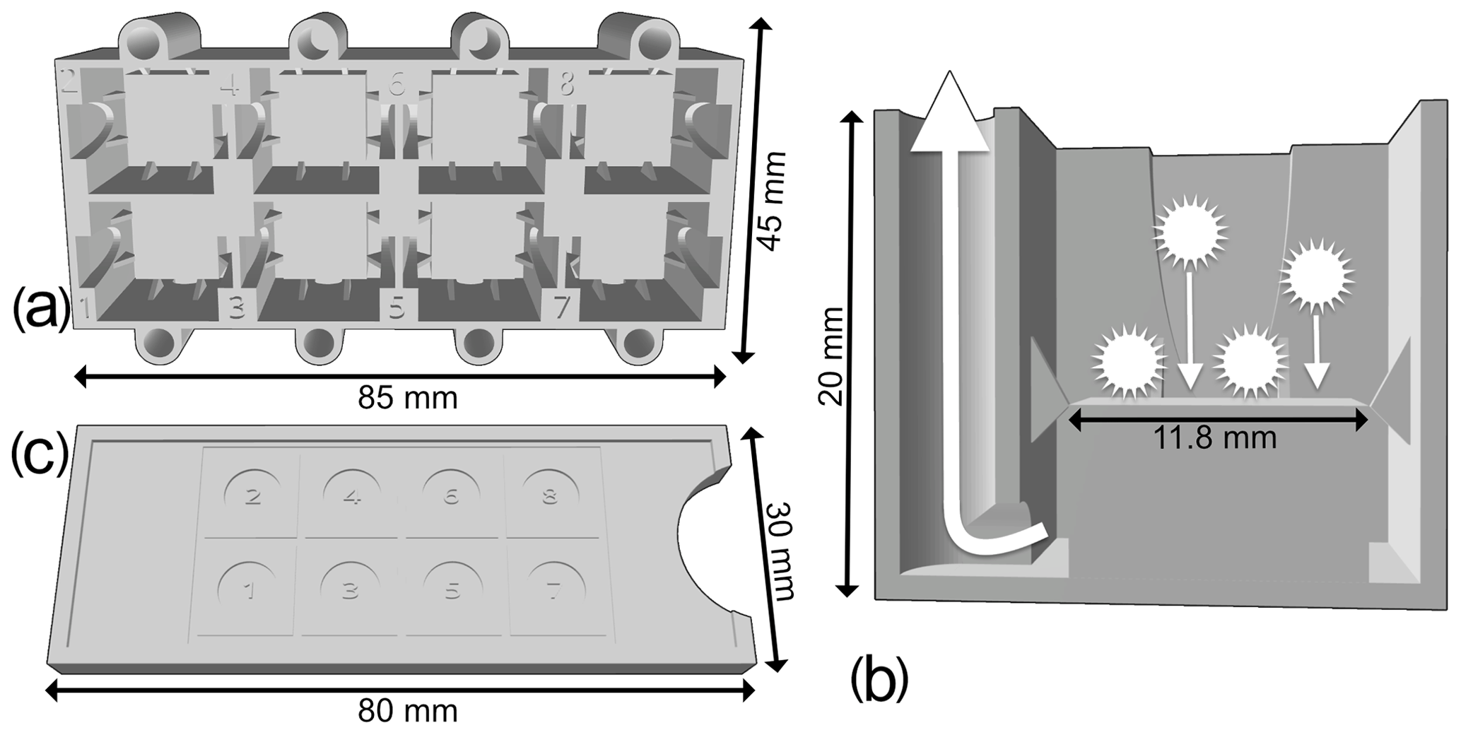
Figure 1 (a) Upper view of the new 3D-printed decanter, showing eight tanks. (b) Cross section of a single tank of the new 3D-printed decanter. (c) Upper view of the slide guide.

A random settling technique was preferred to a standard smear slide preparation, as the objective of this study is a detailed quantitative faunal analysis with investigation of the relative abundances of each taxon (Sanfilippo et al., 1985). Indeed, a random settling technique provides a more uniform distribution of the residue, resulting in less clumped particles, which make it easier to capture digital images of each specimen. The new decanter minimizes the loss of material, and a slide guide (Fig. 1c) can also be used to align cover slides. During development, various shapes and sizes of tank were tested, and the one presented herein was the best compromise between the quantity of sample material required, the loss of residue that would not settle on the slide and the quantity of microfossil residue recovered. This method is an improved version of the original random settling method developed by Moore (1973); adapted to radiolarian studies by Boltovskoy (1998), which provided an even and random distribution of the shells on a slide; and modified by Beaufort et al. (2014) to mount up to eight samples on a single micropalaeontological glass slide. The use of this new device is simple: a 12 mm × 12 mm cover slide is placed in the middle of each tank and maintained centred by the fins; a solution containing radiolarians in suspension for each sample is then poured onto each tank; and after a few minutes of settling on the cover slides, water is vacuumed out from each hole.

The new radiolarian slide preparation protocol is carried out using the following steps (nos. 2 to 7 have been adapted from a similar procedure used to process limestone and calcareous sediments):

1. weigh the sediment;

2. put about 1 g of sediment (depending on the abundance of radiolarians) in a 200 mL beaker and add a few drops of distilled water to disaggregate it;

3. add a few millilitres of 37 % hydrochloric acid (HCl) until the end of the effervescence;

4. add a more few drops of 37 % HCl to ensure the end of the effervescence;

5. pour the solution and rinse the beaker over a 50 µm sieve;

6. clean the residues in the sieve using a pressure sprayer until they appear whitish;

7. rinse the residues using distilled water;

8. weigh a clean glass storage vial;

9. pour the residues from the sieve to the vial using distilled water;

10. once the residues have decanted, remove the excess water using a pipette;

11. place the vial into the oven (about 50 ^∘C) until the residues are dry;

12. weigh the vial again to calculate the weight of the recovered residues;

13. gently tap the vial to unstick the residues from the bottom of the vial;

14. put a 12 mm × 12 mm licked or flame-burned cover slide into one tank of the decanter;

15. take about 0.6 to 1 mg of siliceous residue and drop it onto 3.5 mL of distilled water;

16. shake this solution to suspend the residue and quickly pour it into the corresponding tank;

17. wait until the residues have decanted (a few seconds to minutes) and slowly vacuum out the water from the hole (Fig. 1b);

18. place the decanter in the oven (about 50 ^∘C) to dry the cover slide;

19. when dry, remove the cover slide from the tank using plastic tweezers and glue it to a standard glass slide (76 mm × 26 mm) using optical glue (e.g. NOA81, refractive index of 1.56).

Regarding step no. 2, the reader should consider the fact that the absolute abundance of radiolarians varies massively in sediment samples from various parts of the ocean. Thus, the amount of sediment dissolved into HCl should be customized according to the expected abundance.

Regarding step no. 15, for a 12 mm × 12 mm cover slide, 0.6 mg of residue corresponds to the best compromise between having a sufficient number of radiolarian specimens and them touching or overlapping too much (see Fig. S1 in the Supplement). This is desirable as touching specimens can often not be individually segmented from images, leading to “double” images containing two or more specimens, which cannot be easily classified or assigned to a species count. Distilled water was preferred to ethanol as it leads to less clustering of specimens.

The volume above the cover slide in the tank corresponds to about 45 % of the total volume of the tank. According to the average weight of a radiolarian specimen (about 0.5 µg Takahashi and Honjo, 1983), the 0.6 mg of siliceous residue after chemical treatment should then contain about 1200 radiolarians, if it is not “contaminated” by other siliceous particles, of which about 600 should fall on the cover slide, thereby resulting in at least 300 specimens that should be available for identification (the minimum required to characterize an assemblage by most of the statistical studies, e.g. Fatela and Taborda, 2002). This was confirmed by our tests that showed an average of 473 complete identifiable radiolarian specimens per sample (or at least exhibiting more than 50 % of their shell), including at least the medullary shells for spumellarians, and the cephalis and thorax for nassellarians (excluding specimens touching each other and broken specimens). Depending on the goal and accuracy of your study, this issue can be easily addressed in the sample preparation by pouring a solution of the same sample into the eight tanks of the decanter (or more or less tanks according to the abundance of radiolarian in the sediment). This way, no changes are required for the image acquisition part of the workflow Other testing found that Norland Optical Adhesive NOA81 glue was preferred to other mounting media, such as NOA74 or Naphrax, due to its refractive index, consistency and long-term preservation. Due to the glue's viscosity, air bubbles can be trapped in some perforated-type shells, which are common in Collosphaeridae for example. Although not ideal, images of specimens containing bubbles that were still recognizable were retained in the database in order to integrate this variability into the neural network. Although time-consuming, metal coating (using C or Au/Pd, for example) is also a very efficient way of increasing contrast prior to mounting specimens on the slides. The darkfield illumination technique was too inconsistent in the images produced, meaning that further tests were not carried out.

2.3 Automated image acquisition

Particular emphasis was placed on acquiring high-quality slide images, as being able to recognize different radiolarian species depends on having clearly visible features. However, it has to be noted that, no matter the image quality, very small features that can be taxonomically important (for example bladed vs. cylindrical spines) are likely to be difficult for the network to learn, as the morphological variability between every picture of each class is likely to play a more important role before the network can focus on such small features. For each radiolarian microscopic slide, the eight cover slides (corresponding to eight samples) are automatically and consecutively imaged using a Leica DMR6000 B automated transmitted light microscope (200 × magnification using a HCX PL FLUOTAR 20 × magnification Leica lens) and a Hamamatsu ORCA-Flash4.0 LT camera, controlled via a LabVIEW (National Instruments) interface. The microscope parameters were set as follows: an intensity of 10, a depth of field of 38, an aperture of 33 and the condenser was lowered by 9 mm from the glass slide. The LabVIEW acquisition software parameters were set as follows: an exposure of 9 ms and a gain of 1. These settings provided the maximum contrast between the glass shells and their mounting medium.

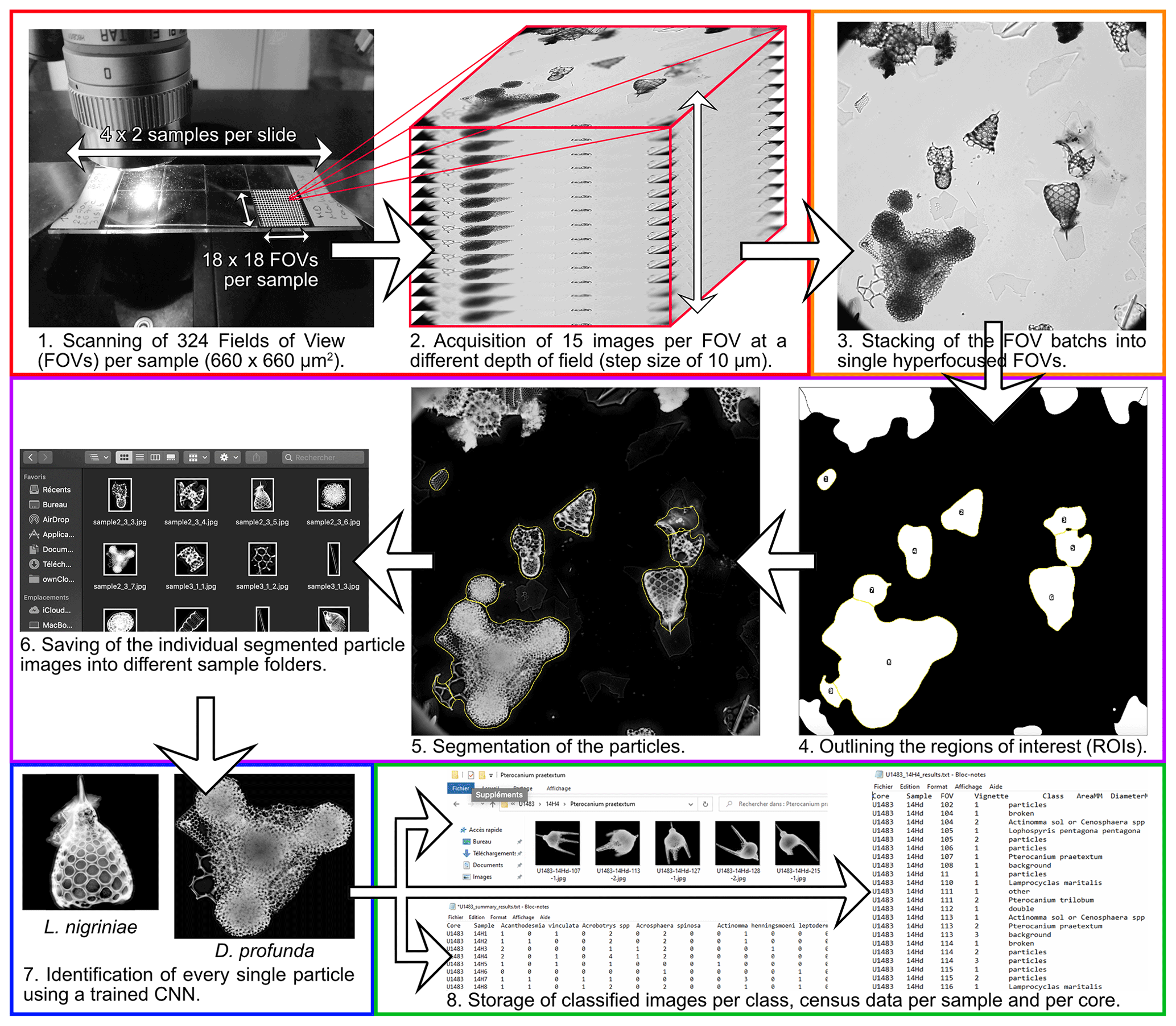
Figure 2 Automated radiolarian image acquisition, processing and identification workflow. Panels 1 and 2 (red rectangle) show the automated acquisition steps. Panel 3 (orange rectangle) shows the automated FOV image stacking step. Panels 4, 5 and 6 (purple rectangle) show the automated FOV image processing and segmentation steps. Panel 7 (blue rectangle) shows the automated recognition step. Panel 8 (green rectangle) shows the automated export of classified images, census counts and morphometric measurements.

For each sample, 324 fields of view (18 × 18 FOVs of 660 µm  × 660 µm each within each 12 mm × 12 mm cover glass) were imaged using a multifocal technique (Fig. 2). For each FOV, 15 images were acquired by incrementally stepping the Z focus position through the microscopic slide (step size of 10 µm) to cover a total focal distance of 150 µm, which corresponds to the thickness of most radiolarian species. This acquisition step takes exactly 1 h per sample, equating to 8 h per slide.

2.4 Automated image processing and segmentation

Image processing and segmentation is performed via a second LabVIEW interface. For each FOV, the batch of 15 images is automatically stacked using Helicon Focus 7 (Helicon Soft) and saved following a CoreName-SampleName-FOVNumber.jpg pattern (Fig. 2). As the shells are outlined by the different refractive indices between the shell and the mounting medium, we did not experienced any identification issue with regard to the stacking step, even with small and/or delicate shells. Every stacked FOV image is then processed and segmented into individual specimen images using a custom plug-in (AutoRadio_Segmenter.ijm) developed for the ImageJ/Fiji software (V1.52n Schneider et al., 2012). Regarding specimens that are cut between two FOVs, if a part of the shell contains the first chambers (usually for Nasselaria) it would be identified as the correct class, and the second part would be identified as “broken”, in order to prevent a double identification in the correct class. The processing steps are as follows:

1. open a stacked FOV image;

2. subtract its background;

3. adjust the minimum and maximum greyscale value to increase its contrast;

4. invert the image and create a mask;

5. threshold it in order to binarize it;

6. blur it and threshold it again to obtain the overall shape of each particle;

7. separate particles that are in contact with each other (require the configurable BioVoxxel “Water Irregular Features” plug-in, available at https://github.com/biovoxxel/BioVoxxel_Toolbox, last access: 17 November 2020);

8. define regions of interest (ROIs) for each particle;

9. restore ROIs corresponding to every particle on the original FOV image;

10. create a square vignette for each particle;

11. save it into the corresponding “Core” folder and “Sample” subfolder.

Each sample results in approximately 1000 to 3000 individual segmented vignettes after the automated image processing and segmentation step.

2.5 Database building and CNN training

ParticleTrieur is a dedicated software program developed at CEREGE (Marchant et al., 2020) that enables the operator to visualize and assign vignettes to manually defined classes; the program uses the k-NN (k-nearest-neighbours) algorithm to aid in identification by self-learning and progressively suggesting identification once enough radiolarian pictures are identified (the reader is referred to Marchant et al. (2020) for more information). Using this software, a large dataset of radiolarian taxa images (called the AutoRadio Database) was progressively built (the current version of the database used in this study can be downloaded from http://microautomate.cerege.fr/dat, last access: 17 November 2020, and is freely accessible online as a catalogue at https://autoradio.cerege.fr/database/, last access: 17 November 2020). It is currently composed of 21 746 images, corresponding to 132 classes/taxa. Each class contains between 1 and about 1000 images.

Once labelled, this database was used to train a CNN (convolutional neural network) for the automated taxonomical identification of radiolarian vignettes resulting from the automated microscope image acquisition, processing and segmentation steps. The best results were obtained using a ResNet50 topology (residual nets with a depth of 50 layers; He et al., 2015) with added cyclic (Dieleman, 2016) and gain layers (resnet50_cyclic_gain_tl; see Marchant et al., 2020, for a detailed description of the network), greyscale images resized to 256 px × 256 px, a batch size (number of images presented per training iteration) of 64, 30 epochs and four drops for the adaptive learning rate (ALR) system, and augmentation (Marchant et al., 2020). This training process lasts about 30 min and generates two files that can then be used for automated recognition (network_info.xml and frozen_model.pb files).

2.6 Automated taxonomic identification

Once individual vignettes of radiolarian specimens are generated and saved during the ImageJ processing and segmentation step, they are automatically opened in ParticleTrieur using its server mode, which is controlled by the second LabVIEW interface. These vignettes are then automatically assigned to a class using the trained CNN. Following this, individual vignettes are automatically moved into folders corresponding to their core and sample and into subfolders corresponding to their assigned class. Using one microscope, about 8000 individuals from two slides (16 cover slides corresponding to 16 samples) can be imaged per day (about 500 specimens per sample, from the original 1000 to 3000 vignettes per sample). This fully automated stacking, processing, segmentation and identification step takes about 50 min per sample and operates in parallel to the image acquisition step.

Two types of data are then automatically exported (Fig. 2):

1. For each sample, a “sample results” file is generated that assembles metadata and morphometric measurements. Each taxonomic ID is then returned to the LabVIEW interface and indexed with its corresponding vignette name (also containing the core, sample, FOV and vignette numbers in each column) into a .txt file for each vignette (in each row). For each specimen, morphometric measurements, such as “Area”, “Diameter”, “Major Axis”, “Minor Axis”, “Circularity”, “Roundness”, “Solidity” and “Eccentricity” are also automatically appended to the .txt file.

2. For each core, census data counts of each sample are automatically compiled. A “core results” file is generated during this process where the abundance of each taxon (in column) for each sample (in row) is automatically incremented.

3 Results and discussion

3.1 Description of the database

Of the 21 746 images used to construct the database, 132 morphoclasses (morphological classes) were created. Of all these classes, 124 belong to Neogene to Quaternary radiolarian taxa (116 classes corresponding to species or groups of two to three species and containing 11 126 images, 7 classes corresponding to genera and containing 1932 images, and 1 corresponding to family and containing 677 images) and are part of the Spumellaria families Actinommidae, Coccodiscidae, Heliodiscidae, Litheliidae, Pyloniidae, Spongodiscidae, and Tholoniidae; and of the Nassellaria families Artostrobiidae, Cannobotryidae, Carpocaniidae, Collozoidae, Plagiacanthidae, Pterocorythidae, Theoperidae and Trissocyclidae (see Fig. 3, which includes some example images). Eight non-radiolarian classes (corresponding to “background”, “broken” specimens, air “bubble”, “diatom”, “double”, “porous fragments”, siliceous “particles”, and “spicule” and containing 8011 images) were also defined to train the network to recognize these non-radiolarian images that usually represent half to four-fifths of the total vignettes.

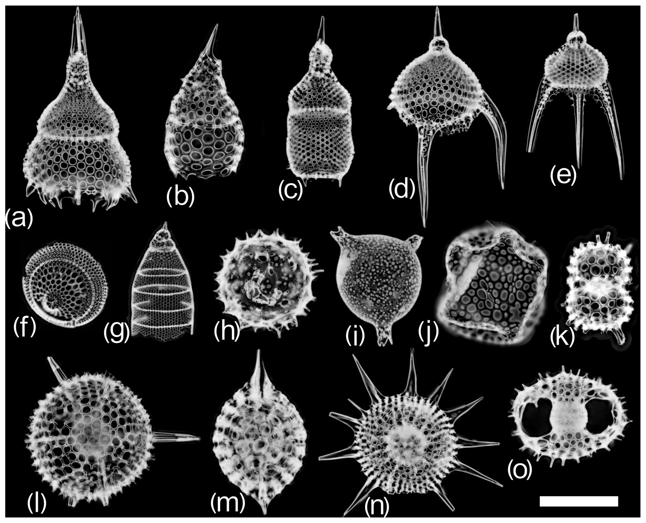
Figure 3 Examples of radiolarian vignettes generated by the automated acquisition, processing and recognition workflow for (a) Lamprocyclas maritalis, (b) Lamprocyrtis hannai, (c) Theocorythium trachelium, (d) Pterocanium trilobum, (e) Pterocanium praetextum, (f) Eucecryphalus sestrodiscus, (g) Eucyrtidium acuminatum/hexagonatum, (h) Acrosphaera spinosa, (i) Solenosphaera chierchiae, (j) Collosphaera tuberosa, (k) Didymocyrtis tetrathalamus tetrathalamus, (l) Hexacontium spp., (m) Stylatractus neptunus, (n) Heliodiscus asteriscus and (o) the Tetrapyle octacantha group. The scale bar represents 100 µm.

An extensive overview of the existing Neogene to Quaternary literature was used for the taxonomy and identification of each class as well as to define our assemblages and the observed taxa as accurately as possible (including Ling and Anikouchine, 1967; Nigrini and Moore, 1979; Nigrini and Lombari, 1984; Boltovskoy and Jankilevich, 1985; Caulet and Nigrini, 1988; Takahashi, 1991; Abelmann, 1992; Boltovskoy, 1998, 1999; Sharma et al., 1999; Nigrini and Sanfilippo, 2001; Itaki et al., 2003; Kamikuri et al., 2009; Zhang et al., 2009; Lazarus et al., 2015; Matsuzaki et al., 2015; Motoyama et al., 2016; Boltovskoy et al., 2017; Matsuoka, 2017; Zhang and Suzuki, 2017; Sandoval, 2018). Synonymies were also taken into account, especially regarding the work of Boltovskoy (1998, 1999). This means that a few species were regrouped into a single class when a significant morphological gradation was observed and when the limit between the considered species was blurry (e.g. Eucyrtidium acuminatum and E. hexagonatum; Sithocampe arachnea and S. lineata; Actinomma henningsmoeni and A. leptodermum). Conversely, ontogenetic stages are clearly visible in numerous species-level classes and, once sufficiently imaged, could be distinguished into separated classes. All manual taxonomic IDs during the building of the database were reviewed by a radiolarian taxonomy expert (Giuseppe Cortese) to ensure consistent and accurate identifications.

3.2 Results of the CNN training

One of the best ways to assess the efficiency of a trained CNN is to look at its confusion matrix (Fig. 4; the original excel spreadsheet is available in the Supplement, see Table S1). Right before the training step, the dataset is automatically split into two subsets: one is the training set, and the other is the test set. The data split chosen for this study is one-fifth. This means that four-fifths of the original images are used for training (training set) while the remaining one-fifth (test set) of the original images is used for testing the CNN efficiency by calculating several indices. The efficiency results are then represented by the overall accuracy Eq. (1), precision Eq. (2), recall Eq. (3) and the individual recall for each class, with these terms defined as follows:

$$\begin{array}{}\text{(1)}& \text{Accuracy}={\displaystyle \frac{\text{number of images correctly classified}}{\text{total number of images}}}\end{array}$$

Figure 4 Confusion matrix showing the overall and individual accuracy, precision and recall for the 109 trained classes. Squared groupings correspond to radiolarian families. This figure is also available as a scrollable Excel spreadsheet in the Supplement (Table S1).

The accuracy is the overall performance of the system regardless of class. If you select a random image from the dataset and classify it, the overall accuracy is the probability (in percent) that the returned classification is correct.

$$\begin{array}{}\text{(2)}& \begin{array}{rl}& \text{Precision}=\\ & {\displaystyle \frac{\text{number of images that were classified as class }N\text{ and actually belong to class }N}{\text{total number of images classified as class }N}}\end{array}\end{array}$$

Precision is a metric for a specific class: it is the probability (in percent) that an image classified as class N is actually from class N, divided by the total number of images classified as class N.

$$\begin{array}{}\text{(3)}& \begin{array}{rl}& \text{Recall}=\\ & {\displaystyle \frac{\text{number of images in class }N\text{ that were correctly classified}}{\text{total number of images in class }N}}\end{array}\end{array}$$

For a specific class, recall is the probability (in percent) that a random image from class N is correctly classified, divided by the number of images belonging to class N. Recall is basically the accuracy of a single class. Individual recall scores for each class are visible in the confusion matrix (Fig. 4) as the percentage of class N (row) that was identified as various classes (column). For example, for the first row “Acanthodesmia vinculata”, 95 % of the images belonging to this class were correctly identified, whereas 5 % were classified as “Lophospyris pentagona pentagona”. If the CNN training was perfect, the diagonal should only exhibit “100” values. The single overall recall and precision scores are the respective values averaged across all the classes.

During the CNN training, all classes containing less than 10 images (corresponding to rare species that currently lack images) were automatically fused into a single “other” class. Of the original 132 classes, 109 classes (including 101 radiolarian classes from the middle Miocene to the Quaternary, and 8 non-radiolarian classes) were then trained to be recognized with a current overall precision accuracy of just above 90 % (90.1 %) over every class. The average precision is above 85 % (85.6 %), and the average recall is about 81 % (80.7 %). A closer look at the matrix shows that classes with a low recall score usually correspond to classes containing an insufficient number of images (rare species, difficult to get on slide, that would require a significant amount of samples to be processed before enough individual images were generated), usually less than 30 images (e.g. Axoprunum acquilonium: 20 %, contains only 25 images; Clathrocanium coarctatum: 50 %, contains only 12 images), while several hundred images per class are usually recommended. More images, at least 150 (ideally 300) in total for each class, as defined above, are then likely to increase the recall and accuracy of these under-represented classes. To this end, the database will be updated and populated gradually through the automated processing of new samples. As the objective of this database is to be open-access and interactive, people are encouraged to send and/or add pictures of these under-represented classes and to send any suggestion to improve the taxonomical framework of the database (see the online contact form at https://autoradio.cerege.fr/contact/, last access: 17 November 2020).

While the ability of the network to distinguish between morphologically and taxonomically very dissimilar taxa is very strong (Fig. 4: almost every value outside of the squares corresponds to family groupings in the confusion matrix that are 0; most of the specimens are usually assigned to their correct family: Actinommidae: 93 %; Coccodiscidae: 93 %; Heliodiscidae: 100 %; Lithelidae: 88 %; Pyloniidae: 95 %; Spongodiscidae: 96 %; Artostrobiidae: 97 %; Cannobotryidae: 95 %; Carpocaniidae: 93 %; Collozoidae: 99 %; Plagiacanthidae: 87 %; Pterocorythidae: 98 %; Theoperidae: 96 %; Trissocyclidae: 99 %), we also tested its ability to distinguish between morphologically very similar forms, usually corresponding to closely related taxa (species or genera) by computing the accuracy of each radiolarian family present in the database (using the number of specimens of the test set and recall score for each class). Overall, the intra-family accuracy for each family is very high (Actinommidae: 80 %; Coccodiscidae: 89 %; Heliodiscidae: 100 %; Lithelidae: 84 %; Pyloniidae: 90 %; Spongodiscidae: 89 %; Artostrobiidae: 93 %; Cannobotryidae: 95 %; Carpocaniidae: 93 %; Collozoidae: 91 %; Plagiacanthidae: 85 %; Pterocorythidae: 92 %; Theoperidae: 93 %; Trissocyclidae: 94 %). For each class, the top three classes that were most often confused with it are summarized in Table S2. Most of the misclassification usually occurs with classes of the same family or with the “broken” class, where a specific part of the investigated class might be recognized (e.g. part of a cephalis or part of a thorax, although always incomplete).

As attempts to use genus- or higher-level taxa as radiolarian proxies in palaeoenvironmental research have yielded almost no useful signals, we tried to integrate as many classes corresponding to species-level taxa in our network as possible. However, the whole workflow is a compromise between distinguishing as many species as possible and trying to maintain good accuracy for each class, which mostly depends on the growing number of images in each of them. The more images that are progressively added to the database, the more accurate the identification will be, and the closer to the species-level we will be able to go for each class. It should be noted that geographic variation in morphology that might affect the system's performance has not yet been taken into account, although the addition of samples from other locations to cover the species-specific variation in morphology linked with spatial distribution is planned. The morphological variation over time (within lineages, for example) should not affect the system's performance, as each class contains images of specimens usually covering the species' lifespan.

3.3 Accuracy of the trained CNN on a random set of samples

In order to test the reliability and reproducibility of our trained CNN on actual samples, a slide with eight cover slides containing siliceous particles from eight random samples with variable radiolarian abundances was selected. Four Quaternary samples (400 to 6400 years BP) from Core U1488A and four Miocene samples (10.116 to 10.694 Ma) from Core U1483 (both from IODP Expedition 363) were then prepared, and their identification scores were computed. This slide was automatically imaged, FOV pictures were automatically segmented and individual vignettes were automatically identified using the trained CNN. After a manual verification of every automated identification, six indices were computed: (1) the percentage of radiolarian images recognized as radiolarians (Fig. 5a); (2) the percentage of radiolarian images recognized as the correct radiolarian taxa (Fig. 5c); (3) the percentage of non-radiolarian images recognized as non-radiolarian particles (Fig. 5b); (4) the percentage of non-radiolarian images recognized as the correct particle class (Fig. 5d); (5) the percentage of non-radiolarian images recognized as radiolarian (non-radiolarian false positive; Fig. 5e); and (6) the percentage of radiolarian recognized as non-radiolarian (radiolarian false positive; Fig. 5f).

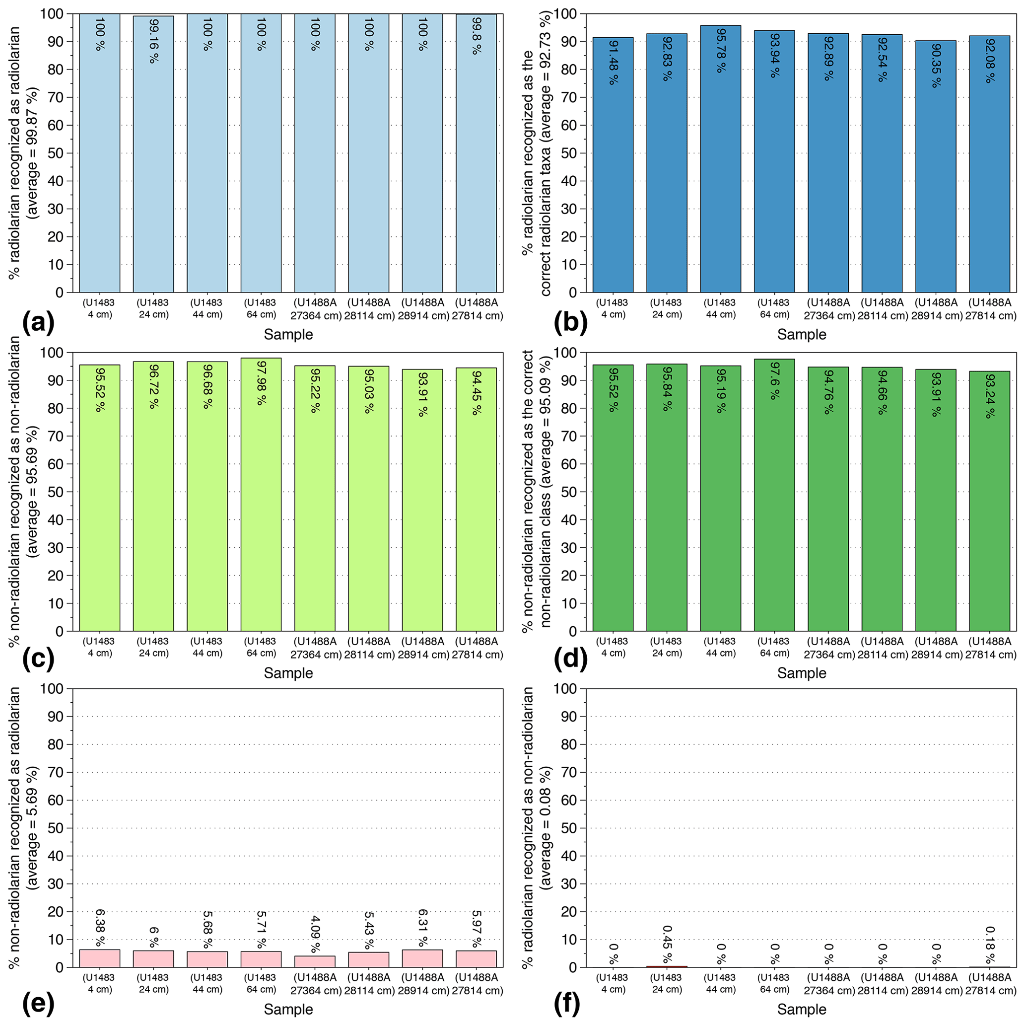
Figure 5 Identification indices evaluated on eight Quaternary and Miocene random samples recovered from cores U1483 and U1488A (IODP Expedition 363).

Overall, 7800 vignettes were identified and manually checked among the eight samples containing between 444 and 1502 images each. The abundance of radiolarians ranged from 176 to 697 specimens per sample. The results show that the six indices exhibit very close values between the eight samples. On average, the proportion of radiolarians actually recognized as radiolarian is very high, about 100 % (Fig. 5a), and the proportion of radiolarians identified as the correct radiolarian taxa is about 93 % (Fig. 5b). Thus, almost all radiolarian images are recognized as radiolarian with a 7 % error regarding their species identification. Regarding the non-radiolarian images, more than 95 % are recognized as non-radiolarian (Fig. 5c) and, again, about 95 % are assigned to the correct class (Fig. 5d).

False positive identifications were also investigated and are relatively low. Among all of the images identified as non-radiolarians, only 0.08 % should be assigned to radiolarians, and among all the images automatically recognized as radiolarians, about 6 % are non-radiolarian images. Within these 6 %, most of the non-radiolarian images confused with radiolarians exhibit radiolarian features and correspond to the non-radiolarian classes “broken” and “double” that either contain incomplete radiolarians or radiolarians touching each other and cannot be assigned to a single species. These false positives are then usually assigned, in the “broken” class case, to the species partially present in the image, or in the “double” class case, to one of the species that can be distinguished.

3.4 Interest for biostratigraphic studies

The new automated radiolarian identification workflow is also of interest for biostratigraphic studies, as radiolarian faunal events, such as first occurrences (FOs) and last occurrences (LOs) of radiolarian taxa (about 30 zones were defined for the Cenozoic; Sanfilippo et al., 1985) are commonly used for biostratigraphic studies of the Neogene to Quaternary interval (Nigrini, 1971; Lazarus et al., 1985; Johnson et al., 1989; Moore, 1995; Sanfilippo and Nigrini, 1998; Nigrini and Sanfilippo, 2001; Vigour and Lazarus, 2002; Nigrini et al., 2005; Kamikuri et al., 2009; Kamikuri, 2017). The known stratigraphic ranges of the 101 middle Miocene to Quaternary radiolarian classes included in our database can then be used to automatically assign an age to any sample, according to the composition of its radiolarian assemblage. This operative workflow, which is automated from the image acquisition to the census counts and can suggest an age for the processed sample, could thus significantly contribute to the field of biostratigraphy.

3.5 Application to other datasets and other studies

To test the potential application and limits of our trained CNN on existing sets of images, we compiled various individual images of radiolarians from the literature including un-stacked optical microscope images and SEM images. We then performed a simple colour inversion of the optical microscope image to obtain white specimens on a dark background. Of the hundred images tested, about half were correctly recognized, whereas the others were mostly assigned to the “background” class, likely due to the blurry shell edges of the un-stacked images, and to the “broken” class, as only part of the shell was probably recognized. While this 50 % accuracy on a random set of un-stacked optical microscope and SEM images may seem relatively low and arbitrary, it is very encouraging and promising for the development of future and extensive neural networks for automated radiolarian recognition regardless of the imaging method.

4 Conclusions

A new automated radiolarian workflow was developed and consists of a sequence of six steps:

1. a new microscopic slide preparation protocol to enable an efficient automated image acquisition on transmitted light microscopes and decrease the loss of material, as this can limit the investigation of samples where radiolarians are scarce;

2. automated microscope image acquisition that can automatically image microscopic slides bearing up to eight samples (324 FOV images per sample) at different focal depths (15 images per FOV, every 10 µm in depth);

3. automated stacking of each batch of FOV images (using depth maps) to generate a single clear FOV with clearly distinct radiolarian specimens;

4. automated FOV image processing (contrast enhancement, B&W inversion) and segmentation to generate individual images for every radiolarian specimen;

5. automated radiolarian recognition using a CNN, as well as calculating morphometric measurements;

6. automated export of census data per sample (usually about 500 radiolarian images per sample) and storage of radiolarian images in folders corresponding to their taxonomic identification for every sample.

The whole procedure is then entirely automated from the image acquisition to the census counts and only requires the operator to prepare the micropalaeontological slides and put them under the microscope. Thus, the operative workflow described in this study can perform complex, tedious, time-consuming tasks such as taxonomic identification and census counts by producing reliable, reproducible and accurate results. Moreover, as the system can identify most of the common Miocene to Quaternary species, taxonomic specialists can focus on unknown and poorly documented forms. This workflow is achieved using a polyvalent and extensive radiolarian image database (currently 21 746 images) and a ResNet CNN trained using transfer learning for modern and Neogene radiolarian identification. The CNN is currently able to recognize 109 classes with an average precision of about 90 %, which is an overall score that was also obtained on a test performed on eight random samples containing about 7800 images.

Although the database already incorporates 124 radiolarian taxa, the main limitation of our system is that it does not yet cover the entire scope of radiolarian diversity, which can be relatively high in tropical and subtropical areas (about 500 species), but only equatorial sediments, although these sediments exhibit numerous worldwide species. In order to continue to increase its efficiency, more images are required, particularly for rare species and from other oceanic regions. The more samples that are processed using the automated workflow, the more images will be progressively added to the database. To this end, the database was also made open-access and interactive in order to rapidly increase the number of images (see online at https://autoradio.cerege.fr), especially for rare species where the recall score is relatively low, which is most likely due to low numbers of training images for these taxa.

This new workflow and associated CNN has the potential to make palaeoclimate studies more approachable and feasible, along with biostratigraphy for very long sequences. It can be easily installed in other laboratories equipped with an automated microscope, as most of our developments are made open-access. The radiolarian census data can then be used to investigate the radiolarian assemblages' variability for biostratigraphical purposes and to develop, apply and improve existing assemblage-based palaeoenvironmental proxies such as SSTs (e.g. radiolarian-based palaeotemperatures for the late Quaternary, Cortese and Abelmann, 2002; subtropical (ST) index, Lüer et al., 2008; radiolarian temperature index (RTI), applied to Miocene samples, Kamikuri, 2017) and palaeoproductivity (e.g. upwelling radiolarian index (URI), Caulet et al., 1992; water depth ecology index (WADE), Lazarus et al., 2006). It also enables the investigation of evolutionary trends, the appearance of new species and the rate of evolutionary change, which are fascinating topics regarding radiolarians and other microfossil groups.

This dataset and following studies also enable the fast and accurate measurement of numerous morphometric parameters for each vignette that was assigned a class in the automated recognition step. In addition to the previous research applications, the morphometry aspect provides the possibility to investigate the link between the morphological variability of a species or an assemblage through time along a sedimentary record and elaborate and/or test scenarios to explain such variability. This new workflow will now be used on two Neogene to Holocene sedimentary records from IODP Expedition 363 (Hole U1483A and Hole U1488A), recovered in the West Pacific Warm Pool.