Simulating the climate response to atmospheric oxygen variability in the Phanerozoic: a focus on the Holocene, Cretaceous and Permian

The amount of dioxygen (O₂) in the atmosphere may have varied from as little as 5 % to as much as 35 % during the Phanerozoic eon (54 Ma–present). These changes in the amount of O₂ are large enough to have led to changes in atmospheric mass, which may alter the radiative budget of the atmosphere, leading to this mechanism being invoked to explain discrepancies between climate model simulations and proxy reconstructions of past climates. Here, we present the first fully 3-D numerical model simulations to investigate the climate impacts of changes in O₂ under different climate states using the coupled atmosphere–ocean Hadley Centre Global Environmental Model version 3 (HadGEM3-AO) and Hadley Centre Coupled Model version 3 (HadCM3-BL) models. We show that simulations with an increase in O₂ content result in increased global-mean surface air temperature under conditions of a pre-industrial Holocene climate state, in agreement with idealised 1-D and 2-D modelling studies. We demonstrate the mechanism behind the warming is complex and involves a trade-off between a number of factors. Increasing atmospheric O₂ leads to a reduction in incident shortwave radiation at the Earth's surface due to Rayleigh scattering, a cooling effect. However, there is a competing warming effect due to an increase in the pressure broadening of greenhouse gas absorption lines and dynamical feedbacks, which alter the meridional heat transport of the ocean, warming polar regions and cooling tropical regions.

Case studies from past climates are investigated using HadCM3-BL and show that, in the warmest climate states in the Maastrichtian (72.1–66.0 Ma), increasing oxygen may lead to a temperature decrease, as the equilibrium climate sensitivity is lower. For the Asselian (298.9–295.0 Ma), increasing oxygen content leads to a warmer global-mean surface temperature and reduced carbon storage on land, suggesting that high oxygen content may have been a contributing factor in preventing a “Snowball Earth” during this period of the early Permian. These climate model simulations reconcile the surface temperature response to oxygen content changes across the hierarchy of model complexity and highlight the broad range of Earth system feedbacks that need to be accounted for when considering the climate response to changes in atmospheric oxygen content.

1 Introduction

The primary driver of climate over the Phanerozoic is atmospheric CO₂ (Royer et al., 2004). However, atmospheric oxygen content may also have varied across the Phanerozoic. Atmospheric dioxygen (O₂) plays a vital role in the Earth system (Catling et al., 2005), regulating the biosphere through fire ignition (Watson et al., 1978) and metabolism of aerobic biota. Hence, variability in the partial pressure of dioxygen (pO₂, a measure of the mass of O₂ in the atmosphere, assuming N₂ and the volume of the atmosphere have been constant) over time has been invoked as an evolutionary trigger (Berner et al., 2007) of both animals (Falkowski et al., 2005) and plants (He et al., 2012) at many points in the Phanerozoic (Saltzman et al., 2011; Robinson, 1990; Beerling and Berner, 2000; Scott and Glasspool, 2006; Edwards et al., 2017).

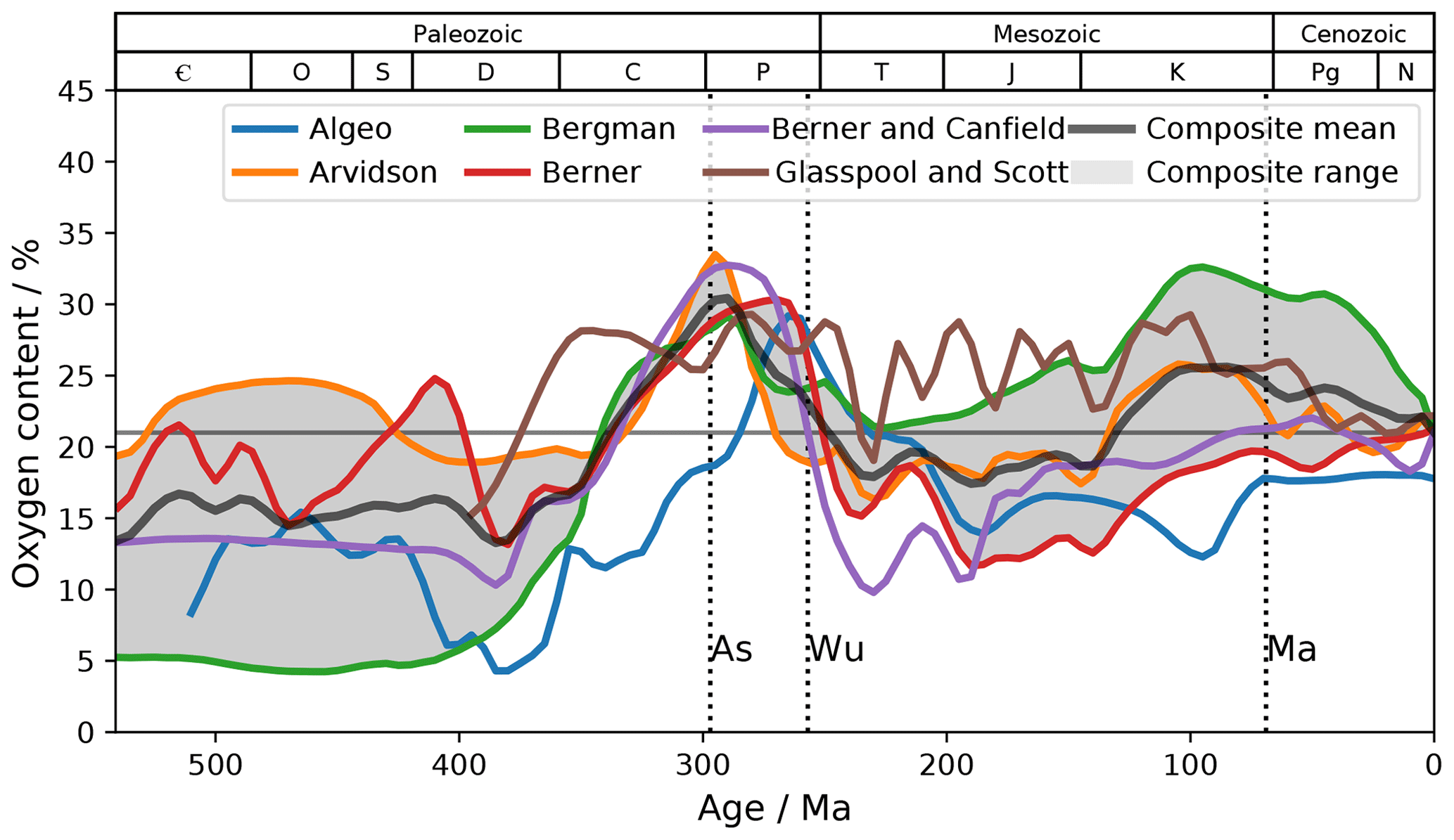
Figure 1 Oxygen content reconstructions in the Phanerozoic from Algeo and Ingall (2007), Arvidson et al. (2013), Bergman et al. (2004), Berner (2009), Berner and Canfield (1989) and Glasspool and Scott (2010). The mean (black line) and range (grey shading) of the Arvidson et al. (2013), Bergman et al. (2004) and Berner (2009) is indicated, as these reconstructions were most consistent with ice core evidence (Stolper et al., 2016). Present-day atmospheric oxygen content is indicated by the solid horizontal grey line. Timings of the palaeo case studies explored in this study are indicated by the dotted vertical lines (As: Asselian, Wu: Wuchiapingian, Ma: Maastrichtian).

While strong biological and geological feedbacks prevent rapid swings in atmospheric oxygen (Catling and Claire, 2005), reconstructions of past atmospheric oxygen content suggest that there have been substantial excursions from the 21 % oxygen content present in today's atmosphere at times in the Phanerozoic eon. These reconstruction methods can be divided into forward and inversion models. Forward models include nutrient/weathering models (Bergman et al., 2004; Arvidson et al., 2013; Hansen and Wallmann, 2003) and isotope mass balance models (Berner, 2009; Falkowski et al., 2005), while inversion models infer oxygen content from proxies such as charcoal (Glasspool and Scott, 2010), organic-carbon-to-phosphorus ratios (Algeo and Ingall, 2007) and plant resin δ¹³C (Tappert et al., 2013). Figure 1 shows the reconstructed oxygen content for a variety of these methods. There is general agreement in the trends in the reconstructions, in that oxygen content increased from 5 % to 25 % in the early Paleozoic to 20 %–35 % in the Permian and subsequently stabilised at levels around 15 %–30 % from the Middle Triassic onward. However, there is uncertainty in the absolute amount of O₂ for the different reconstructions (grey shading in Fig. 1). Indeed, there is support for elevated O₂ by carbon isotope measurements during the Permian (Beerling et al., 2002). However, disagreement is particularly evident in the Mesozoic, with low values simulated by isotope mass balance approaches. Mills et al. (2016) have shown that this could be due to an inappropriate choice of δ¹³C and that adjusting this value with geological constraints leads to a higher reconstructed oxygen content in better agreement with wildfire records. At the time of writing, there are no direct geochemical proxies for atmospheric pO₂ on the Phanerozoic timescale. However, there is isotopic evidence of oceanic oxygenation in steps at approximately 560 (Dahl et al., 2010), 400 (Dahl et al., 2010; Lu et al., 2018) and 200 Ma (Lu et al., 2018). pO₂ in the last 800 000 years has been reconstructed using O₂∕N₂ ratios in ice cores (Stolper et al., 2016). A roughly 7 ‰ decline in pO₂ is consistent with the ability to change oxygen content by the order of a few percent in ∼10 Myr. The reconstructions of Bergman et al. (2004), Arvidson et al. (2013) and Berner (2009) are the most plausible based on ice core data (Stolper et al., 2016). Considering these three models alone would still suggest a large uncertainty in oxygen content for most of the Phanerozoic, except for elevated levels in the late Carboniferous/early Permian and reduced levels in the late Devonian.

Phanerozoic means “visible life” and one of the marked changes to carbon cycling between the Proterozoic and Phanerozoic was caused by the emergence of land plants. The radiation of land plants has led to strong regulation of atmospheric CO₂ and O₂ which both play important roles in photosynthesis. Land plants likely led to a substantial sequestration of carbon in the terrestrial biosphere and possibly led to the Ordovician glaciation (Lenton et al., 2012). Increases in organic carbon sequestration in the aftermath of the evolution of lignin production may also have contributed to the cooling (Robinson, 1989). This fundamental change to the Earth system may have constrained CO₂ levels to between 10 and 200 Pa ever since (Franks et al., 2014). Watson et al. (1978) have argued that strong fire feedbacks prevent large fluctuations in oxygen levels, due to runaway burning at high oxygen levels. However, subsequent experiments using natural fuels support the possibility of the Earth system to support higher oxygen levels (Wildman et al., 2004). Charcoal appears in the fossil record continuously since the late Devonian (∼360 Ma; Algeo and Ingall, 2007; Scott and Glasspool, 2006). This suggests a floor on oxygen levels in the region of 12 % (Wildman et al., 2004) to 16 % (Belcher and McElwain, 2008; Belcher et al., 2010) since then due to limits on ignition.

Variations in pO₂ also have important implications for photosynthesis and therefore the operation of the terrestrial carbon cycle. The primary CO₂-fixing enzyme, RuBisCO, possesses a dual carboxylase–oxygenase function (Smith, 1976). A photosynthetic carboxylase pathway removes CO₂ from the atmosphere, while oxygenation leads to photorespiration and CO₂ evolution. Therefore, increases in pO₂ ought to lead to O₂ outcompeting CO₂ for active sites on the RuBisCO enzyme and leading to a reduction in net primary productivity (less photosynthesis, more respiration). However, photorespiration is likely to be necessary for removal of harmful byproducts in the photosynthetic metabolic pathway (Hagemann et al., 2016), and a recent study suggests that increases in photorespiration may actually promote photosynthesis (Timm et al., 2015). Photosynthesis is itself sensitive to the background CO₂ content (Beerling and Berner, 2000). In addition, temperature modifies the relative solubilities of CO₂ and O₂ (Jordan and Ogren, 1984). Temperature also affects the specificity of RuBisCO for CO₂ (Long, 1991). Therefore, the coevolution of pO₂, pCO₂ and temperature across the Phanerozoic has the capacity to significantly impact the terrestrial carbon cycle.

This paper focuses on investigating the climate impacts of atmospheric mass variation as the result of altering the concentration of O₂. Lower atmospheric mass leads to less Rayleigh scattering so more shortwave radiation reaches the Earth’s surface. This enhances atmospheric convection and the hydrological cycle, which leads to more tropospheric water vapour, further enhancing warming. However, lower atmospheric mass leads to a reduction in the pressure broadening of greenhouse gas absorption lines which should lead to a weaker greenhouse effect and lead to cooling. Previous modelling studies have investigated which factor dominates with conflicting results. Goldblatt et al. (2009) presented radiative–convective model simulations for the Archean (∼ 3 Ga), which suggested that a nitrogen inventory around 3 times larger than present would help to keep the early Earth warm at a time when solar input was only around 75 % of what it is today, potentially solving the “Faint Young Sun” paradox (Feulner, 2012). Charnay et al. (2013) investigated this using a general circulation model (GCM) coupled to a slab ocean and found that for their idealised early Earth simulations they achieved a strong warming (+7 ^∘C) in response to a doubling in atmospheric mass. Poulsen et al. (2015) simulated the climate impacts of changes in O₂ content over a range of 5 %–35 % using the GENESIS climate model with a slab ocean and a continental configuration consistent with the Cenomanian (mid-Cretaceous, 95 Ma) and found the opposite response – lower atmospheric mass at low pO₂ was associated with a strong warming. Subsequent 1-D calculations cast doubt on this result (Goldblatt, 2016; Payne et al., 2016); however, it is plausible that other climate feedbacks such as changes to relative humidity and cloud changes may be important as atmospheric mass changes. These would not be accounted for in 1-D radiative–convective equilibrium simulations. Cloud feedbacks in particular are a good candidate for explaining the discrepancy as cloud feedbacks under CO₂-driven climate change have strong model dependency (Bony et al., 2015). Another feedback which has not been considered is the possible impact of changes in the mechanical forcing of wind on the ocean circulation. In the absence of this effect, Earth’s surface temperature would be 8.7 K cooler (Saenko, 2009) and the Equator-to-pole temperature gradient would be steeper. Wind stress (τ) is parameterised in GCMs as $\mathit{\tau }=\mathit{\rho }\mathit{u}\cdot \mathit{u}$, where ρ is the atmospheric density and u is the surface wind vector. So, as atmospheric density increases, the wind stress on the ocean and therefore ocean heat transport should increase accordingly. Increased meridional heat transport in high-density atmospheres is also supported by an idealised 2-D modelling study of the early Earth (Chemke et al., 2016). As slab ocean models assume a constant or diffusive ocean heat transport, the Charnay et al. (2013) and Poulsen et al. (2015) simulations cannot account for these effects.

As pO₂ variability may alter the radiative budget of the atmosphere, it may also have impacts on the sensitivity of the climate state to CO₂ changes. The equilibrium climate sensitivity (ECS) is a metric for the sensitivity of a climate model to an abrupt doubling of atmospheric CO₂. Understanding this value is important for predictions of both past and future climatic changes. As the radiative forcing of CO₂ is approximately logarithmic with concentration, theoretically the ECS should be constant in time as carbon dioxide changes. However, there is growing evidence that ECS has not been constant over Earth's history (Caballero and Huber, 2013). Changes to the incoming solar radiation (Lunt et al., 2016), palaeogeography (Lunt et al., 2016), CO₂ levels themselves (Meraner et al., 2013) and tropical sea-surface temperatures (Caballero and Huber, 2013) may lead to changes in the sensitivity of a particular climate state to changes in CO₂.

2 Methods and simulations

2.1 Models

The impact of oxygen content variability is investigated with two coupled atmosphere–ocean general circulation models (AOGCMs): Hadley Centre Coupled Model version 3 (HadCM3-BL) and Hadley Centre Global Environmental Model version 3 (HadGEM3-AO).

HadGEM3-AO is an AOGCM (Nowack et al., 2014). The atmosphere component is the UK Met Office Unified Model version 7.3 (Davies et al., 2005) in the HadGEM3-A r2.0 climate configuration (Hewitt et al., 2011). It employs a regular Cartesian grid of 3.75^∘ longitude by 2.5^∘ latitude (N48). In the vertical, 60 hybrid height vertical levels are employed – “hybrid” indicating that the model levels are sigma levels near the surface, changing smoothly to pressure levels near the top of the atmosphere (Simmons and Strüfing, 1983). The model top is 84 km, which permits a detailed treatment of stratospheric dynamics. A 20 min time step is used. The model employs a non-hydrostatic and fully compressible dynamical core, using a semi-implicit semi-Lagrangian advection scheme on a staggered Arakawa C grid (Arakawa and Lamb, 1977). Radiation is represented using the Edwards and Slingo (1996) scheme with six shortwave and nine longwave bands, accounting for the radiative effects of water vapour, carbon dioxide, methane, nitrous oxide and ozone. The Met Office Surface Exchange Scheme 2 (MOSES2) land surface scheme is used (Cox et al., 1999), which simulates atmosphere–land exchanges and hydrology. A fixed present-day vegetation distribution of plant functional types is employed. The ocean component of the model is NEMO-OPA (Nucleus for European Modelling of the Ocean - Océan Parallélisé; Madec, 2008) model version 3.0 (Hewitt et al., 2011), run at a 96 min time step. In the vertical, 31 model levels are used, which increase in thickness steadily between 10 m in the shallowest to 500 m in the deepest layer at 5 km in depth. NEMO employs a tripolar, locally anisotropic grid (ORCA2; Madec, 2008) which permits a more detailed treatment of the north polar region and higher resolution in the tropics. This yields an approximate horizontal resolution of 2^∘ in both longitude and latitude, with an increased resolution of up to 0.5^∘ in the tropics. The sea-ice component of the model is CICE (Los Alamos Community Ice CodE) at version 4.0 (Hunke and Lipscomb, 2008), run at a 96 min time step. This treats sea ice in a five-layer model, allowing the simulation of different ice types. The atmosphere and ocean/sea-ice components exchange fields every 24 h, while NEMO and CICE exchange fields every time step. HadGEM3-AO can be thought of as a close relation to the newest-generation HadGEM3 coupled model that will be used to support the next Intergovernmental Panel on Climate Change (IPCC) assessment (Williams et al., 2018) and so represents the state of science in numerical climate models.

HadCM3-BL (Valdes et al., 2017) is an AOGCM coupled to an interactive vegetation model. The model was originally developed by the United Kingdom Met Office Hadley Centre (Pope et al., 2000) but has since been substantially developed further by the University of Bristol. The atmosphere component of the model employs a regular Cartesian grid of 3.75^∘ longitude by 2.5^∘ latitude. In the vertical, 19 hybrid height vertical levels are employed. A 30 min time step is used. The primitive equation set of White and Bromley (1995) is solved to conserve energy and angular momentum, solved on a staggered Arakawa B grid (Arakawa and Lamb, 1977) in the horizontal. Radiation is represented using the Edwards and Slingo (1996) scheme with six shortwave and eight longwave bands, accounting for the radiative effects of water vapour, carbon dioxide and ozone, amongst other radiative active species. The ocean component of the model employs the same horizontal grid as the atmosphere component of the model, 3.75^∘ longitude by 2.5^∘ latitude. In the vertical, 20 model levels are used which increase in depth from 10 m in the shallowest layer to 616 m in the deepest layer. A time step of 60 min is employed and the ocean and atmosphere components exchange required fields once per day. The ocean component is based on the Cox (1984) model, solving the full primitive equation set in three dimensions. A staggered Arakawa B grid is employed in both atmosphere and ocean models. Sea ice is treated as a zero thickness layer on the surface of the ocean grid. Ice is assumed to form at the base at a freezing point of −1.8 ^∘C but can also form from freezing in ice leads and by falling snow. A simple parameterisation of sea-ice dynamics is also employed (Gordon et al., 2000) and sea-ice formation due to convergence from drift being limited to 4 m thick. Sea-ice albedo is fixed at 0.8 for temperatures below −10 ^∘C, decreasing linearly to 0.5 at 0 ^∘C. The MOSES2.1 land surface model is employed to simulate the fluxes of energy and water between the land surface and the atmosphere (Cox et al., 2000; Essery et al., 2003). TRIFFID (Top-down Representation of Interactive Foliage and Flora Including Dynamics; Cox et al., 1998) predicts the distribution of vegetation using a plant functional type (PFT) approach. TRIFFID is run in equilibrium mode with averaged fluxes calculated over a 5-year period. TRIFFID calculates vegetation properties for five PFTs: broadleaf trees, needleleaf tree, C₃ grass, C₄ grass and shrubs. Grid boxes can contain a mixture of PFTs based on a “fractional coverage co-existence approach” (Valdes et al., 2017). Net primary productivity (NPP) is also calculated, using a photosynthesis-stomatal conductance model (Cox et al., 1998) accounting for a number of factors including atmospheric oxygen content, which affects the photorespiration compensation point (Clark et al., 2011). The predicted vegetation distribution impacts the atmosphere component by altering surface albedo, evapotranspiration and surface roughness.

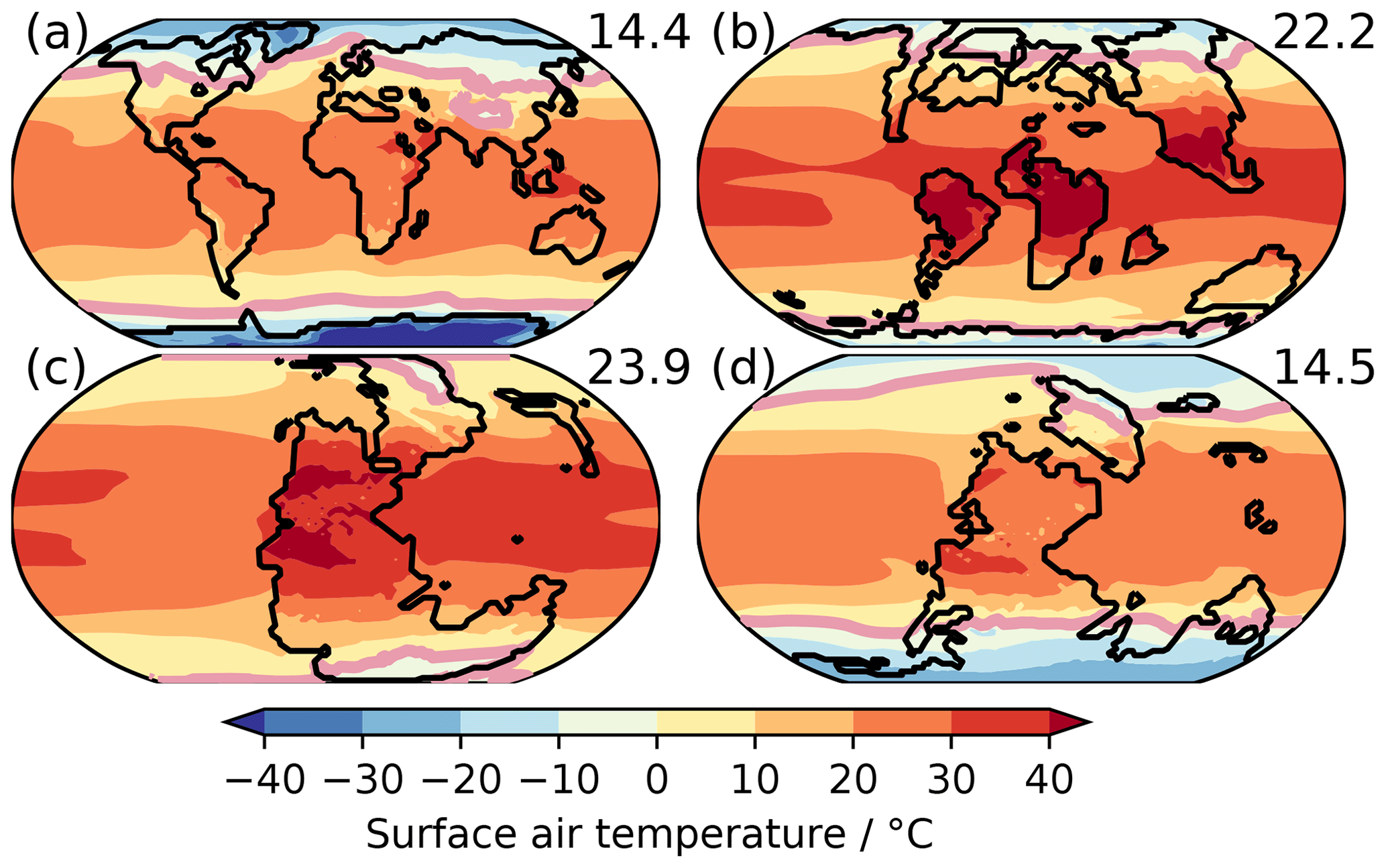
Figure 2 Annual average surface air temperature simulated in (a) PI-CM²¹, (b) Ma-CM²¹, (c) Wu-CM²¹ and (d) As-CM²¹. Global-mean values are indicated in the top right. The 0 ^∘C isoline is indicated in pink. Continental outlines are indicated with a solid black line.

Figure 3 Annual average precipitation simulated in (a) PI-CM²¹, (b) Ma-CM²¹, (c) Wu-CM²¹ and (d) As-CM²¹. Global-mean values are indicated in the top right. Continental outlines are indicated with a solid black line.

2.2 Boundary conditions

Both models simulated the climate response to oxygen variability in a pre-industrial Holocene (PIH) climate. HadCM3-BL was additionally run for three time periods across the Phanerozoic: the Maastrichtian (late Cretaceous, 66.0–72.1 Ma), Wuchiapingian (late Permian, 254.14–259.1 Ma) and the Asselian (early Permian, 295.0–298.9 Ma). The continental reconstructions employed were developed by and are from ©Getech. These reconstructions have been widely employed in a number of previous studies using the HadCM3-BL climate model (e.g. Lunt et al., 2016). All three are periods of time in which models have suggested that atmospheric oxygen may have deviated significantly from the present level of 21 % (see Fig. 1). Modifications were made to alter the oxygen content of the atmosphere by adjusting the mass mixing ratios of major and minor gases, the surface pressure and other physical characteristics of the atmosphere such as the specific gas constant in an analogous way to Poulsen et al. (2015). Figure 2 shows the annual average surface temperatures and Fig. 3 shows the annual average precipitation for the (a) PI-CM²¹, (b) Ma-CM²¹, (c) Wu-CM²¹ and (d) As-CM²¹ simulations.

Table 1 Summary of experiments. Experiment names AA-BBB include the continental configuration (AA) and model used (BBB). Experiment names N × AA-BBB indicate a multiplier of CO₂ with respect to AA-BBB. A star (^*) indicates that the CO₂ multiplier was applied instantaneously and the transient adjustment to climate was analysed for the purpose of a Gregory et al. (2004) analysis.

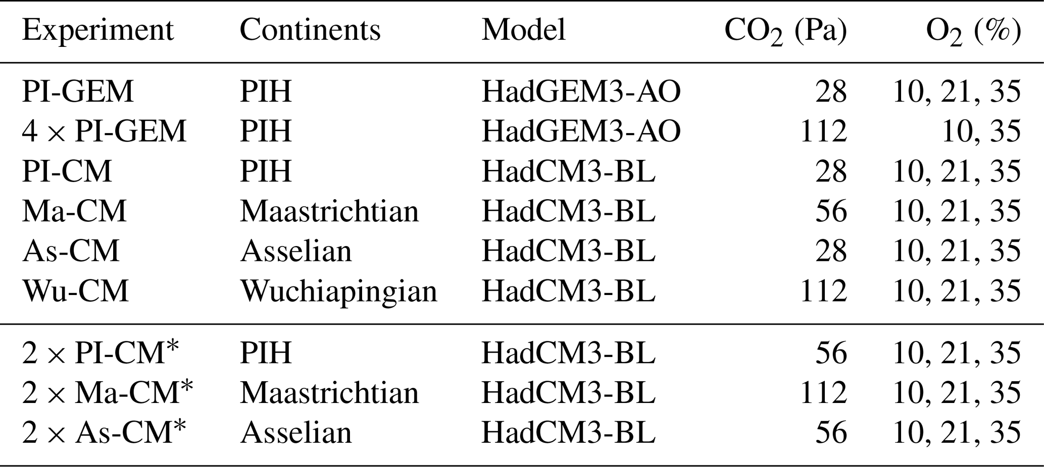
A summary of the experiments performed can be found in Table 1. When an experiment with a particular oxygen content is referred to, it will be indicated in superscript; e.g. EXP²¹ indicates a 21 % oxygen simulation. The 21 % simulations (PI-CM²¹, As-CM²¹, Ma-CM²¹ and Wu-CM²¹) were integrated for 50 model years, as these simulations had already been spun up at that CO₂ content. For 10 % and 35 % pO₂, the model was spun off the 21 % pO₂ simulation and iterated for at least 1000 model years. The 2 × PI-CM^*, 2 × Ma-CM^* and 2 × As-CM^* experiments were spun off from the end of the PI-CM, Ma-CM and As-CM experiments and iterated for 100 years in order to perform a Gregory et al. (2004) analysis. For HadGEM3-AO, model integrations (PI-GEM³⁵, PI-GEM¹⁰, 4 × PI-GEM³⁵ and 4 × PI-GEM¹⁰) were performed for 300 model years with a 10× acceleration of the deep ocean to reduce the time for equilibrium, then integrated for a further 500 years to spin up the shallow ocean without acceleration. The last 50 years were used for model analysis.

Pre-Quaternary pCO₂ is poorly constrained due to the absence of glacial ice; however, there is growing evidence that CO₂ is unlikely to have been significantly higher than the order of hundreds of Pa since the radiation of land plants (Breecker et al., 2010; Franks et al., 2014). For the Maastrichtian, 56 Pa is used in agreement with stomatal proxy-based reconstructions (Steinthorsdottir and Pole, 2016). For the Asselian, 28 Pa is used in agreement with carbonate and fossil plant reconstructions (Montañez et al., 2007). For the Wuchiapingian, 112 Pa is used (Brand et al., 2012).

1-D atmospheric chemistry simulations have simulated higher O₃ column with increasing pO₂ (Kasting et al., 1979; Payne et al., 2016). More detailed 2-D model simulations, which capture critical latitudinal gradients in photolysis and zonal-mean transport (Hadjinicolaou and Pyle, 2004; Haigh and Pyle, 1982), support a monotonically increasing ozone column with increasing pO₂ (Harfoot et al., 2007). However, simulated ozone column was more sensitive to N₂O levels than pO₂ (Harfoot et al., 2007). In addition, while column ozone reduces at low pO₂ in Harfoot et al. (2007), there are increases in ozone concentration in the tropical tropopause region where the radiative effect of O₃ is stronger (Forster and Shine, 1997). Changes in lightning are important for understanding future changes in tropospheric ozone (Banerjee et al., 2014); however, they are subject to considerable uncertainty (Finney et al., 2018). There may be more lightning at high pO₂ due to a higher pO₂∕pN₂ ratio or less due to reduced convection (Goldblatt et al., 2009). Low pO₂ may also enhance isoprene emissions (Rasulov et al., 2009), which could enhance tropospheric ozone and alter cloud properties (Kiehl and Shields, 2013). Ozone is also sensitive to changes in CH₄ and N₂O; the changes to inventories of these chemically active species on the Phanerozoic timescale (Beerling et al., 2009, 2011) are highly uncertain. Ozone is also sensitive to dynamical changes. Given these large uncertainties in possible changes to chemical sources, reactivity and transport, we neglected including changes in atmospheric ozone concentration in these simulations. However, we recommend that follow-up work should focus on this specific question in detail. In HadGEM3-AO, the mass of tropospheric and stratospheric ozone is fixed at PIH values simulated by Nowack et al. (2014) using a tropopause height-matching scheme. This prevents a rising tropopause leading to stratospheric levels of ozone existing in the troposphere, particularly in the 4 × PI-GEM experiments. Not accounting for a rising tropopause has been found to artificially increase climate sensitivity (Heinemann, 2009) and initial tests not accounting for this led to instability for 4 × PI-GEM¹⁰. In HadCM3-BL, tropospheric ozone is set to 6 ppbv and stratospheric ozone is set to 1.66 ppmv for the 21 % simulations. These values are adjusted to conserve total ozone mass in the alternative pO₂ scenarios.

2.3 Data

Data for the Cenomanian (Poulsen et al., 2015) 21 % O₂ and 10 % O₂ simulations were obtained from https://www.ncdc.noaa.gov/paleo/study/18776 (last access: 21 February 2018). At the time of writing, the 35 % simulation contained missing data, so it was not used for analysis.

2.4 1-D energy balance model

A 1-D energy balance model (EBM) has been used to deconvolve the contributions from changes in different parts of the climate system. This 1-D EBM approach has been applied to zonal-mean quantities for climate simulations of the Eocene by Heinemann et al. (2009) following Budyko (1969) and Sellers (1969):

$$\begin{array}{}\text{(1)}& \begin{array}{rl}& {\mathrm{SW}}_{\mathrm{t}}^{\downarrow }\left(\mathit{\varphi }\right)\left[\mathrm{1}-\mathit{\alpha }\left(\mathit{\varphi }\right)\right]-{\displaystyle \frac{\mathrm{1}}{\mathrm{2}\mathit{\pi }{R}^{\mathrm{2}}\cos \left(\mathit{\varphi }\right)}}{\displaystyle \frac{\partial F\left(\mathit{\varphi }\right)}{\partial \mathit{\varphi }}}\\ & =\mathit{ϵ}\left(\mathit{\varphi }\right)\mathit{\sigma }{T}_{\mathrm{s},\mathrm{ebm}}^{\mathrm{4}}\left(\mathit{\varphi }\right),\end{array}\end{array}$$

where SW${}_{\mathrm{t}}^{\downarrow }$ is the incident shortwave radiation at the top of the atmosphere, ϕ is the latitude, α is the surface albedo, R is the radius of Earth, ϵ is the effective surface emissivity, and T_s, ebm is the EBM surface temperature (Heinemann et al., 2009). $\frac{\partial F\left(\mathit{\varphi }\right)}{\partial \mathit{\varphi }}$ is the divergence of total meridional heat transport and is given by

$$\begin{array}{}\text{(2)}& {\displaystyle \frac{\partial F\left(\mathit{\varphi }\right)}{\partial \mathit{\varphi }}}=-\mathrm{2}\mathit{\pi }{R}^{\mathrm{2}}\cos \left(\mathit{\varphi }\right)\left({\mathrm{SW}}_{\mathrm{t}}^{\mathrm{net}}\left(\mathit{\varphi }\right)+{\mathrm{LW}}_{\mathrm{t}}^{\mathrm{net}}\left(\mathit{\varphi }\right)\right),\end{array}$$

where SW${}_{\mathrm{t}}^{\mathrm{net}}$ and LW${}_{\mathrm{t}}^{\mathrm{net}}$ are the net top-of-atmosphere shortwave and longwave radiative fluxes, respectively (positive downward; Heinemann et al., 2009). Solving for T_s, ebm, the EBM surface temperature for each latitude can be calculated using zonal- and annual-mean radiative fluxes from the GCM. Where clear-sky radiative fluxes are also available, cloud radiative effects can be deconvolved from clear-sky radiative effects. The clear-sky albedo α_c and clear-sky effective surface emissivity ϵ_c can be calculated by

$$\begin{array}{}\text{(3)}& {\displaystyle }{\mathit{\alpha }}_{\mathrm{c}}={\displaystyle \frac{{\mathrm{SW}}_{\mathrm{t},\mathrm{c}}^{\uparrow }}{{\mathrm{SW}}_{\mathrm{t}}^{\downarrow }}},{\mathit{ϵ}}_{\mathrm{c}}={\displaystyle \frac{{\mathrm{LW}}_{\mathrm{t},\mathrm{c}}^{\uparrow }}{{\mathrm{LW}}_{\mathrm{s}}^{\uparrow }}},\end{array}$$

where SW${}_{\mathrm{t},\mathrm{c}}^{\uparrow }$ is the upward top-of-atmosphere clear-sky shortwave radiative flux and LW${}_{\mathrm{t},\mathrm{c}}^{\uparrow }$ is the upward top-of-atmosphere clear-sky longwave radiative flux. When considering the temperature change between two experiments, the contributions from different components can be quantified by calculating T_s, ebm with different combinations of components from each experiment (Heinemann et al., 2009).

2.5 Climate sensitivity

To estimate the climate sensitivity to CO₂ changes, the linear regression methodology of Gregory et al. (2004) is employed. This assumes a linear relationship between the changes in global, annual-mean radiative imbalance at the top of the atmosphere (N, W m⁻²) and surface temperature anomalies (T_s, ^∘C):

$$\begin{array}{}\text{(4)}& {\displaystyle }N=F+\mathit{\xi }\mathrm{\Delta }{T}_{\mathrm{s}},\end{array}$$

where ξ is the effective climate feedback parameter ($\mathrm{W}{\mathrm{m}}^{-\mathrm{2}}{}^{\circ }{\mathrm{C}}^{-\mathrm{1}}$) and F is the effective forcing (W m⁻²) accounting for fast climate adjustments and effective radiative forcing. The effective ECS is then ΔT_s when N=0. While there are weaknesses of this approach, particularly due to non-linearities in ξ as ΔT_s changes (Armour et al., 2013; Li et al., 2013), the climate response when simulations are continued to equilibrium shows an accuracy to within 10 % (Li and Sharma, 2013). Furthermore, the contributions to ξ and F from longwave (LW) and shortwave (SW), clear-sky (CS) and cloudy-sky (CRE) components can be decomposed by a linear decomposition as

$$\begin{array}{}\text{(5)}& {\displaystyle }F=F_{\mathrm{CS},\mathrm{SW}}+F_{\mathrm{CS},\mathrm{LW}}+F_{\mathrm{CRE},\mathrm{SW}}+F_{\mathrm{CRE},\mathrm{LW}}\end{array}$$

for the effective forcing and

$$\begin{array}{}\text{(6)}& {\displaystyle }\mathit{\xi }={\mathit{\xi }}_{\mathrm{CS},\mathrm{SW}}+{\mathit{\xi }}_{\mathrm{CS},\mathrm{LW}}+{\mathit{\xi }}_{\mathrm{CRE},\mathrm{SW}}+{\mathit{\xi }}_{\mathrm{CRE},\mathrm{LW}}\end{array}$$

for the effective climate feedback parameter.

3 Results

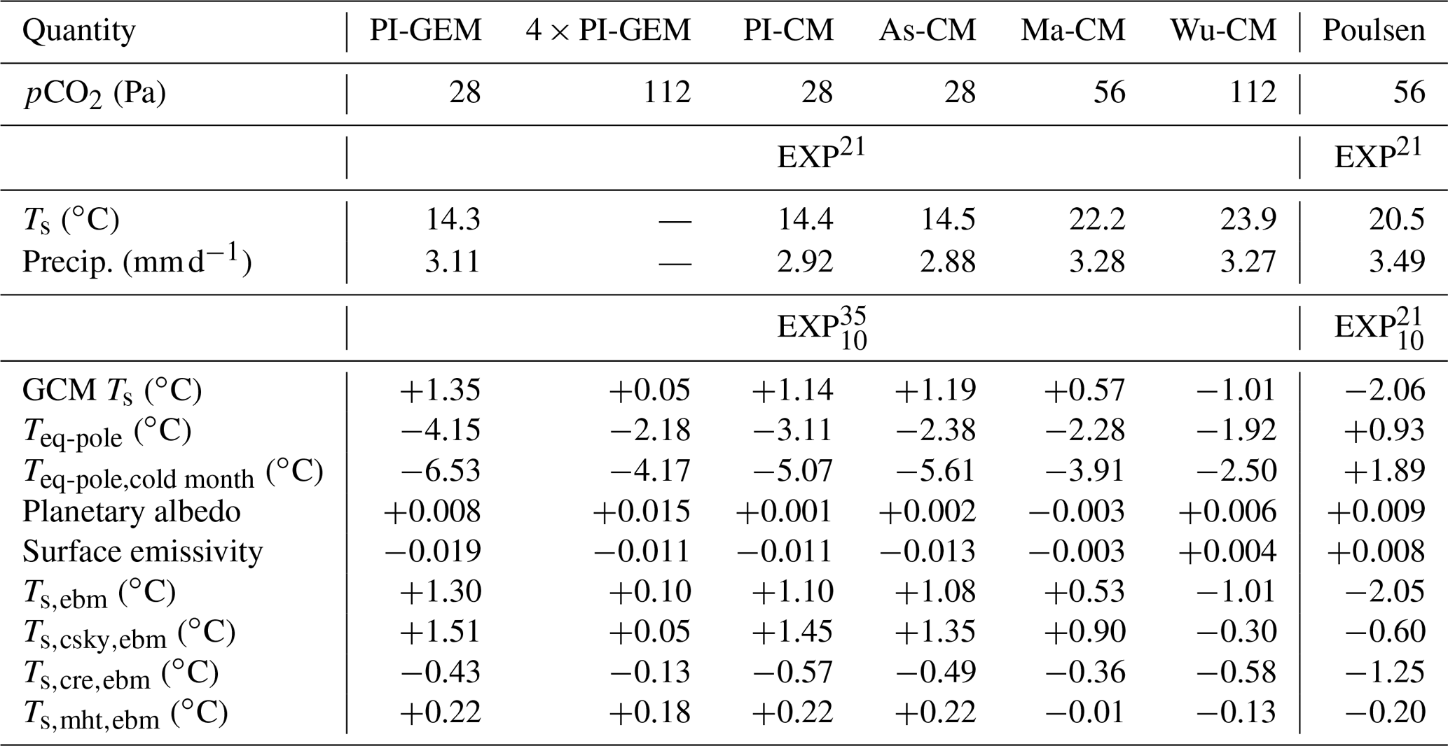
Where results are presented from a single simulation, the oxygen content for that run is written in superscript, i.e. EXP²¹ indicates a 21 % oxygen simulation. Where results are presented as an anomaly between simulations with different oxygen content, ${\mathrm{EXP}}_{\mathrm{0}}^{\mathrm{21}}$ indicates that the quantity presented is EXP²¹ minus EXP⁰. A summary of results is shown in Table 2.

Table 2 Summary of results for EXP²¹, then EXP${}_{\mathrm{10}}^{\mathrm{35}}$. Where applicable, results calculated for the Poulsen et al. (2015) Cenomanian 21 %–10 % oxygen simulation are also presented. Abbreviations: T_eq-pole (Equator-to-pole surface air temperature gradient), T_{eq-pole,cold month} (Equator-to-pole surface air temperature gradient for cold months), EBM (quantities obtained using a Budyko–Sellers 1-D energy balance model following Heinemann, 2009), T_s,ebm (EBM surface temperature), $T_{\mathrm{s},\mathrm{csky},\mathrm{ebm}}$ (EBM surface temperature change accounting for changes in clear-sky radiative fluxes), $T_{\mathrm{s},\mathrm{cre},\mathrm{ebm}}$ (EBM surface temperature change accounting for changes in cloudy-sky radiative fluxes), $T_{\mathrm{s},\mathrm{mht},\mathrm{ebm}}$ (EBM surface temperature change accounting for changes in meridional heat flux divergence).

3.1 Surface climate

Figure 4 (left) shows the annual-mean surface air temperature differences between the 35 % and 10 % runs. For the pre-industrial Holocene, PI-GEM${}_{\mathrm{10}}^{\mathrm{35}}$ (Fig. 4a) shows a global-mean surface temperature response of +1.50 ^∘C, while PI-CM${}_{\mathrm{10}}^{\mathrm{35}}$ (Fig. 4b) shows a similar global-mean surface temperature response of +1.22 ^∘C. It is worth noting that HadCM3-BL and HadGEM3-AO are not completely distinct climate models, for instance, sharing the Edwards and Slingo (1996) radiation scheme, so this is unlikely to capture the full variability in possible climate model responses. That the results are in reasonable agreement with the 1-D results of Payne et al. (2016), who simulated a temperature response between +1.05 and +2.21 ^∘C depending on assumptions about atmospheric ozone, gives some confidence in the HadCM3-BL and HadGEM3-AO results. Similarly, the As-CM${}_{\mathrm{10}}^{\mathrm{35}}$ (Fig. 4c) case exhibits a global-mean surface temperature response of +1.29 ^∘C. For the warmest climates, a response of −0.82^∘C is simulated for Wu-CM${}_{\mathrm{10}}^{\mathrm{35}}$ (Fig. 4e) and +0.17 ^∘C for 4 × PI-GEM${}_{\mathrm{10}}^{\mathrm{35}}$ (Fig. 4f). In the Ma-CM${}_{\mathrm{10}}^{\mathrm{35}}$ case (Fig. 4d), a global-mean surface temperature response of +0.70 ^∘C is simulated. This suggests that the climate response to pO₂ variability depends on the background climate state.

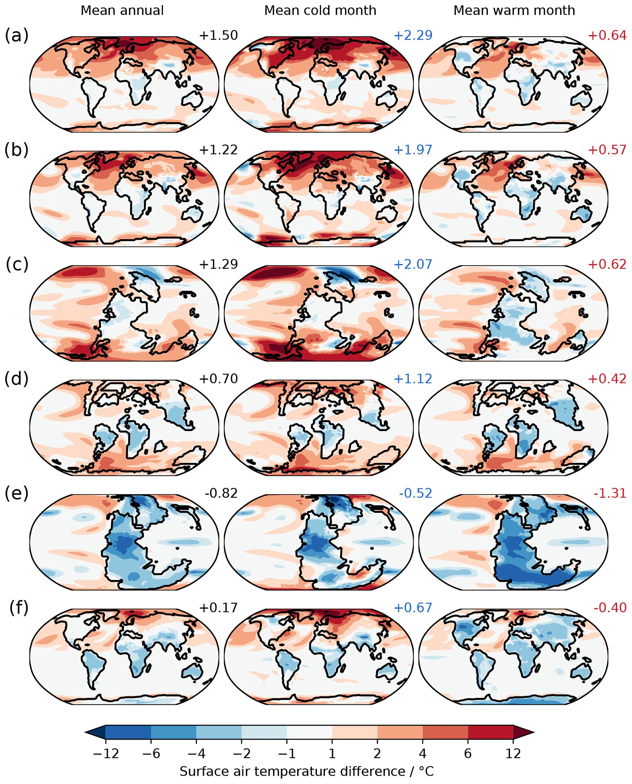
Figure 4 Surface air temperature change for (a) PI-GEM${}_{\mathrm{10}}^{\mathrm{35}}$, (b) PI-CM${}_{\mathrm{10}}^{\mathrm{35}}$, (c) As-CM${}_{\mathrm{10}}^{\mathrm{35}}$, (d) Ma-CM${}_{\mathrm{10}}^{\mathrm{35}}$, (e) Wu-CM${}_{\mathrm{10}}^{\mathrm{35}}$ and (f) 4 × PI-GEM${}_{\mathrm{10}}^{\mathrm{35}}$ in the annual mean (left), cold-month mean (change in the mean grid box temperature of the coldest month in the monthly mean climatology, middle) and warm-month mean (change in the mean grid box temperature of the warmest month in the monthly mean climatology, right). The change in global-mean values (^∘C) are offset to the top right of each plot. Note the strong high-latitude warming in the cold-month mean and tropical cooling in the warm-month mean.

There is a strong seasonal dependence in the surface air temperature response. Considering the changes in coolest average monthly temperature in each grid box (Fig. 4, middle column), the change in cool months dominates the warming response, particularly at high latitudes. By contrast, the warm-month mean is smaller/less negative in all cases (Fig. 4, right). A cooling of continental land masses is evident in the tropics and particularly in the Wu-CM (Fig. 4e) and 4 × PI-GEM (Fig. 4f) cases. These could be in part due to free-air lapse rate changes which should be stronger at high pO₂; as for a given topographic height, the change in pressure is higher for high pO₂, which should lead to a larger temperature reduction with height. The changes to the seasonal cycle are consistent with the radiative changes associated with changing oxygen content. The reduction in incident surface shortwave radiation should have its strongest effect on extratropical temperatures in the summer; therefore, the Rayleigh scattering component will most strongly affect the warm-month temperature. Warming from pressure broadening of greenhouse gas absorption lines as atmospheric mass increases will be most evident in extratropical winter, as with anthropogenic climate change, due to sea-ice and surface heat flux changes (Dwyer et al., 2012). The reduction in the amplitude of the seasonal cycle in temperature simulated by both HadGEM3-AO and HadCM3-BL is therefore supported by a consideration of the changes to atmospheric radiation.

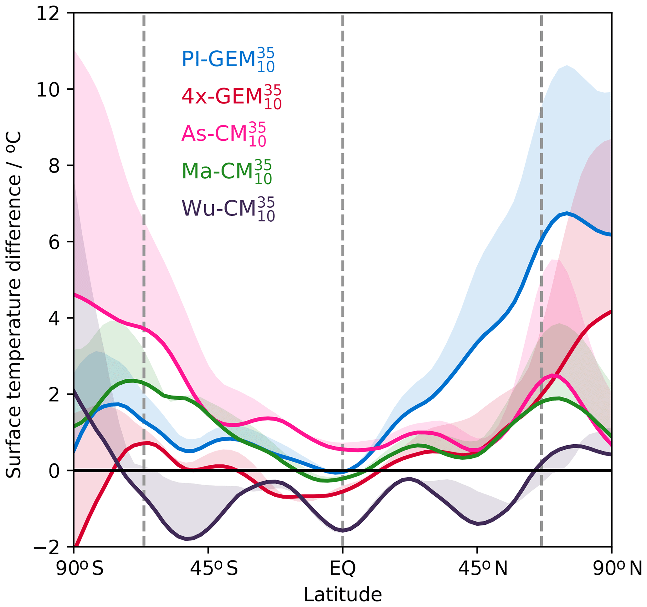
Figure 5 Zonally and annually averaged surface air temperature difference (solid lines) from 10 % to 35 % oxygen content for PI-GEM (blue), 4 × PI-GEM (red), As-CM (pink), Ma-CM (green) and Wu-CM (purple). The difference from the annual mean to cold-month mean for each run is indicated by the shading. Values are smoothed by a Savitzky–Golay filter (Savitzky and Golay, 1964).

The zonal- and annual-mean surface air temperature changes are shown in Fig. 5. The Northern Hemisphere Equator-to-pole temperature gradient is reduced by 6.6 ^∘C in the PI-GEM${}_{\mathrm{10}}^{\mathrm{35}}$ case (blue line) and 4.0 ^∘C in the PI-CM${}_{\mathrm{10}}^{\mathrm{35}}$ case (not shown). The zonal structure of the surface temperature change is similar in the palaeoclimate case studies. In the Maastrichtian, the Equator-to-pole temperature gradient is reduced by 2.0 ^∘C (Ma-CM${}_{\mathrm{10}}^{\mathrm{35}}$) and in the Asselian the Equator-to-pole temperature gradient is reduced by 2.3 ^∘C (As-CM${}_{\mathrm{10}}^{\mathrm{35}}$). The Equator-to-pole temperature gradient reduces even in the Wu${}_{\mathrm{10}}^{\mathrm{35}}$ case despite the reduction in global-mean surface temperatures.

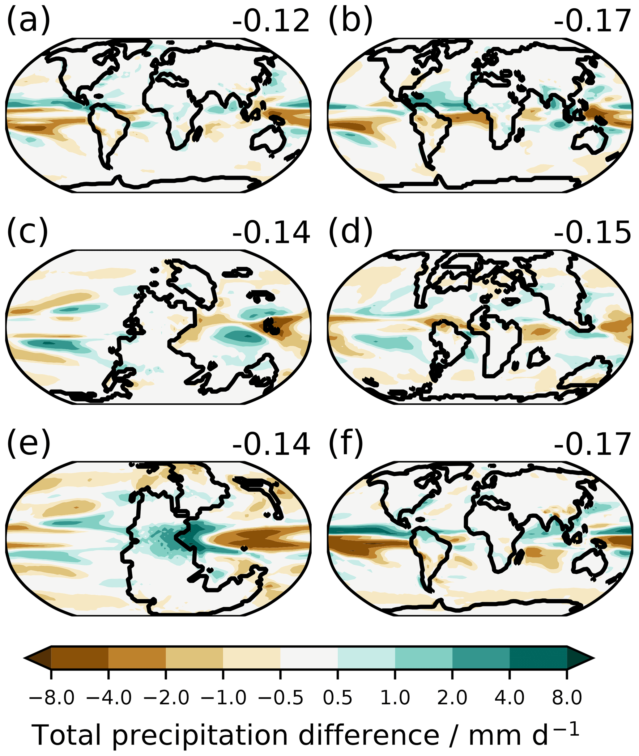
Figure 6 Annually averaged total precipitation change from 10 % to 35 % oxygen content for (a) PI-GEM${}_{\mathrm{10}}^{\mathrm{35}}$, (b) PI-CM${}_{\mathrm{10}}^{\mathrm{35}}$, (c) As-CM${}_{\mathrm{10}}^{\mathrm{35}}$, (d) Ma-CM${}_{\mathrm{10}}^{\mathrm{35}}$, (e) Wu-CM${}_{\mathrm{10}}^{\mathrm{35}}$ and (f) 4 × PI-GEM${}_{\mathrm{10}}^{\mathrm{35}}$. Global-mean values (mm d⁻¹) are offset to the top right of each plot.

The hydrological cycle is also affected by changing oxygen content. Increases in Rayleigh scattering at high pO₂ ought to reduce incident shortwave at the Earth's surface (Poulsen et al., 2015) and inhibit convection (Goldblatt et al., 2009), which should lead to reductions in precipitation. This is analogous to stratospheric sulfate or solar radiation management geoengineering where precipitation is reduced in geoengineering experiments with respect to an unperturbed climate with the same global-mean surface temperature (Irvine et al., 2016). Poulsen et al. (2015) simulated large reductions in precipitation as pO₂ increased in the GENESIS climate model; however, much of this could be explained by the surface temperature changes. Annually averaged precipitation change between the 10 % and 35 % oxygen content runs is shown in Fig. 6. In all cases, increasing oxygen content leads to a decline in global-mean total precipitation, despite the increase in surface temperatures, however, with strong regional differences. For PI-GEM (Fig. 6a), PI-CM (Fig. 6b) and 4 × PI-GEM (Fig. 6f), there is a clear northward shift in the tropical rainbelts. A northward shift in the Intertropical Convergence Zone (ITCZ) would be consistent with stronger warming in the Northern Hemisphere due to Bjerknes compensation (Bjerknes, 1964; Broccoli et al., 2006). Heat transport is more hemispherically symmetric in the Maastrichtian, Asselian and Wuchiapingian cases so latitudinal ITCZ shifts are not evident. While global precipitation is reduced in Wu-CM³⁵, the increase in ocean–land temperature contrast leads to a significant increase in tropical land precipitation. Despite the increases in global-mean surface temperatures simulated for most cases, precipitation is still reduced in all simulations.

Comparing the surface temperature and precipitation response between HadCM3-BL and HadGEM3-AO suggests that the model responses are broadly consistent. A grid-box-by-grid-box comparison of annual-mean surface air temperature and precipitation anomalies for PI-GEM${}_{\mathrm{10}}^{\mathrm{35}}$ vs. PI-CM${}_{\mathrm{10}}^{\mathrm{35}}$ is presented in Fig. S1 in the Supplement. The largest discrepancy in surface air temperature response between the two models occurs for the largest temperature changes simulated by HadGEM, which are strongest in Northern Hemisphere polar regions. This could be linked to differences in the representation of polar climate processes and amplification by polar ice feedbacks between the two models. There is broad consistency in cold- and warm-month means (Fig. 4a and b) with stronger warming in the cold-month mean and terrestrial cooling in the warm-month mean.

3.2 Energy balance decomposition

The drivers of the changes in surface temperature can be understood by decomposing the terms which contribute to surface temperature change in a 1-D energy balance model following Heinemann et al. (2009). For PI-CM${}_{\mathrm{10}}^{\mathrm{35}}$, these results are shown in Fig. 7. These show that the 1-D EBM can reasonably capture the temperature response in the HadCM3-BL simulations, with slight errors (where the black and grey lines are not overlapping) evident in the polar regions. This could be due to averaging over the polar rows in the HadCM3-BL model. There are positive contributions to the surface temperature change in the clear-sky emissivity and albedo at the poles. This is consistent with the increase in pressure broadening of absorption lines and the simulated reduction in sea-ice extent. By contrast, extrapolar contributions to clear-sky albedo provide a negative contribution to the temperature change which is consistent with an increase in Rayleigh scattering which would be expected to be strongest in the tropics where the maximum in incoming solar radiation is located. Combined, the clear-sky component of the temperature change is +1.45^∘C and the cloudy-sky component is −0.35^∘C. This suggests that HadCM3-BL supports a cloud feedback which acts to cool the climate at high pO₂ and partially offset the clear-sky temperature changes.

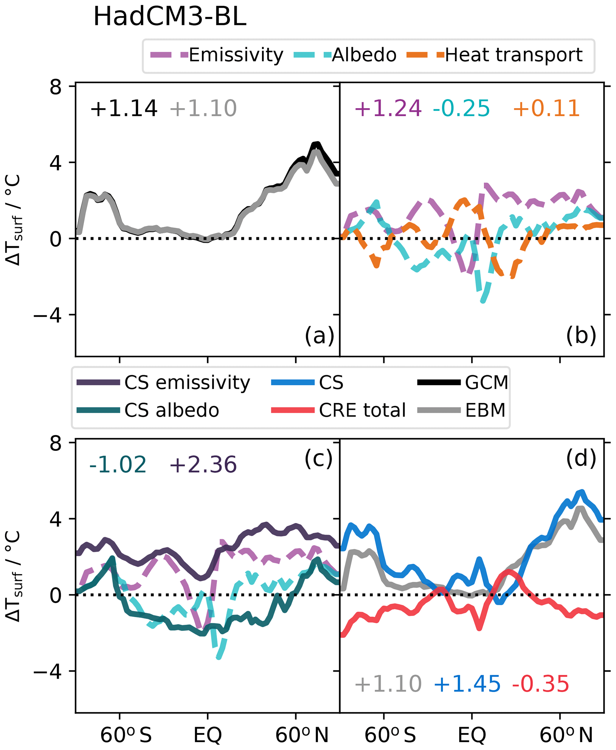
Figure 7 The 1-D EBM decomposition for PI-CM${}_{\mathrm{10}}^{\mathrm{35}}$. (a) EBM results (grey) vs. GCM results (black). (b) Decomposition of EBM into the emissivity (purple), albedo (green) and heat transport (orange) components of the temperature change. (c) Clear-sky emissivity (dark purple) and clear-sky albedo (dark green) components of the EBM. The all-sky components are included for comparison. (d) Decomposition of EBM into the total clear-sky (blue), cloudy-sky (red) and all-sky (grey) components.

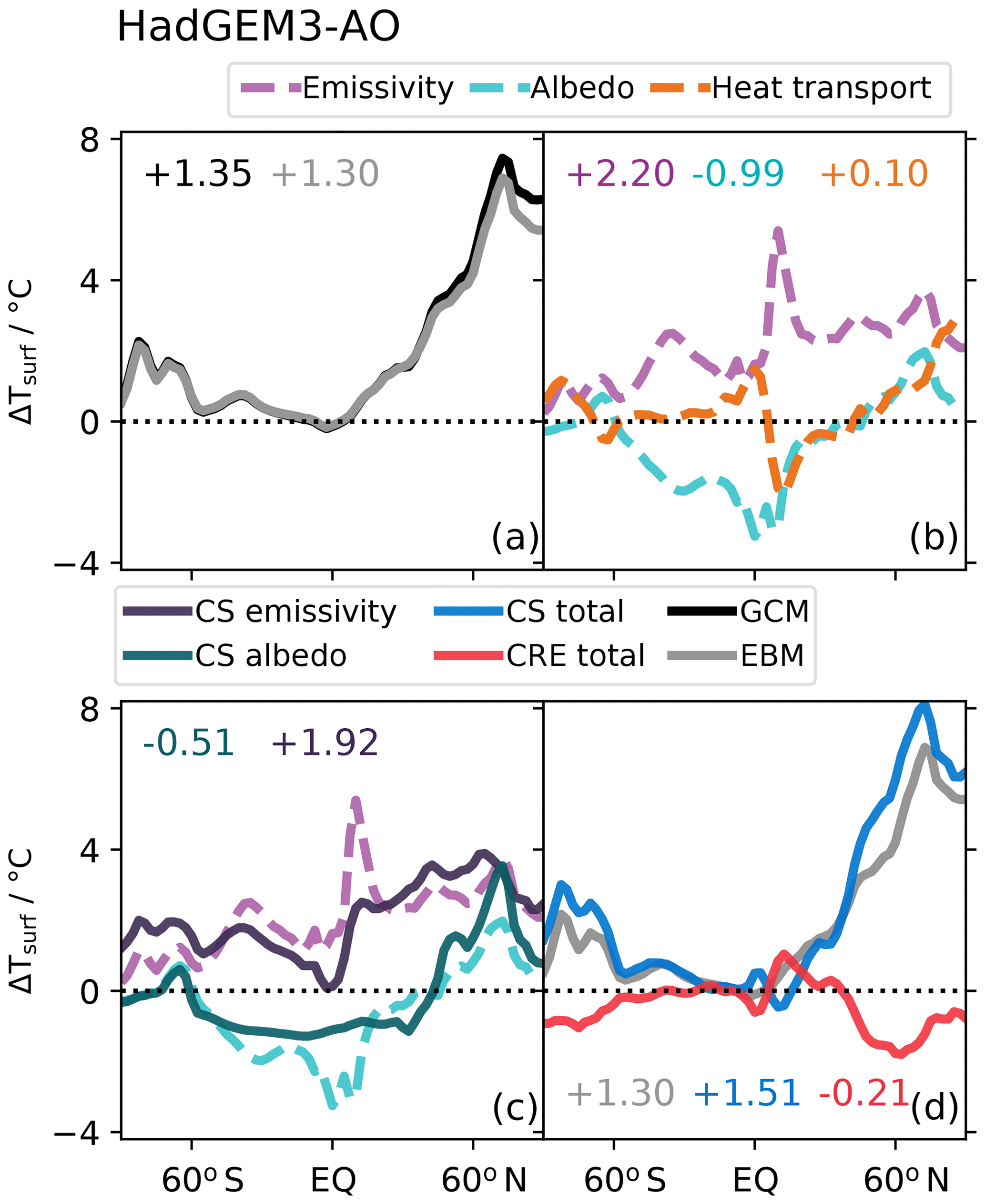
Figure 8 1-D EBM decomposition for PI-GEM${}_{\mathrm{10}}^{\mathrm{35}}$. (a) EBM results (grey) vs. GCM results (black). (b) Decomposition of EBM into the emissivity (purple), albedo (green) and heat transport (orange) components of the temperature change. (c) Clear-sky emissivity (dark purple) and clear-sky albedo (dark green) components of the EBM. The all-sky components are included for comparison. (d) Decomposition of EBM into the total clear-sky (blue), cloudy-sky (red) and all-sky (grey) components.

The same analysis was performed for the HadGEM3-AO PIH simulations. Figure 8 shows that a somewhat weaker cloud feedback is simulated by HadGEM3-AO (−0.21 ^∘C). Clear-sky contributions are slightly stronger (+1.51 ^∘C). The largest differences between the simulations appear in the all-sky albedo and emissivity changes, where there appear to be competing factors which lead to a similar climate response possibly related to partitioning between the longwave and shortwave contributions to the cloud response. This is perhaps unsurprising, as cloud feedbacks to CO₂ changes represent a large uncertainty in future climate change projections, and given the relatively small global-mean temperature changes, a relatively small change in cloud radiative effects has the power to considerably mediate the climate response. However, the qualitative agreement in latitudinal structure of the clear-sky albedo and emissivity changes between these structurally different models gives some confidence that the relevant climate feedbacks are well captured in these simulations.

Analysis of the palaeo case studies (As-CM, Fig. S2; Ma-CM, Fig. S3; Wu-CM, Fig. S4) shows a similar pattern. In all simulations, irrespective of surface temperature response, the clear-sky emissivity is a positive contribution to global-mean surface temperature change, while clear-sky albedo is a more negative contribution. The emissivity contribution becomes less positive as pCO₂ increases from As-CM to Ma-CM to Wu-CM. By contrast, the albedo contribution becomes more negative as pCO₂ increases. This is consistent with the reduction in planetary albedo as sea-ice extent is reduced on the ocean and dark vegetated surfaces increase on the land.

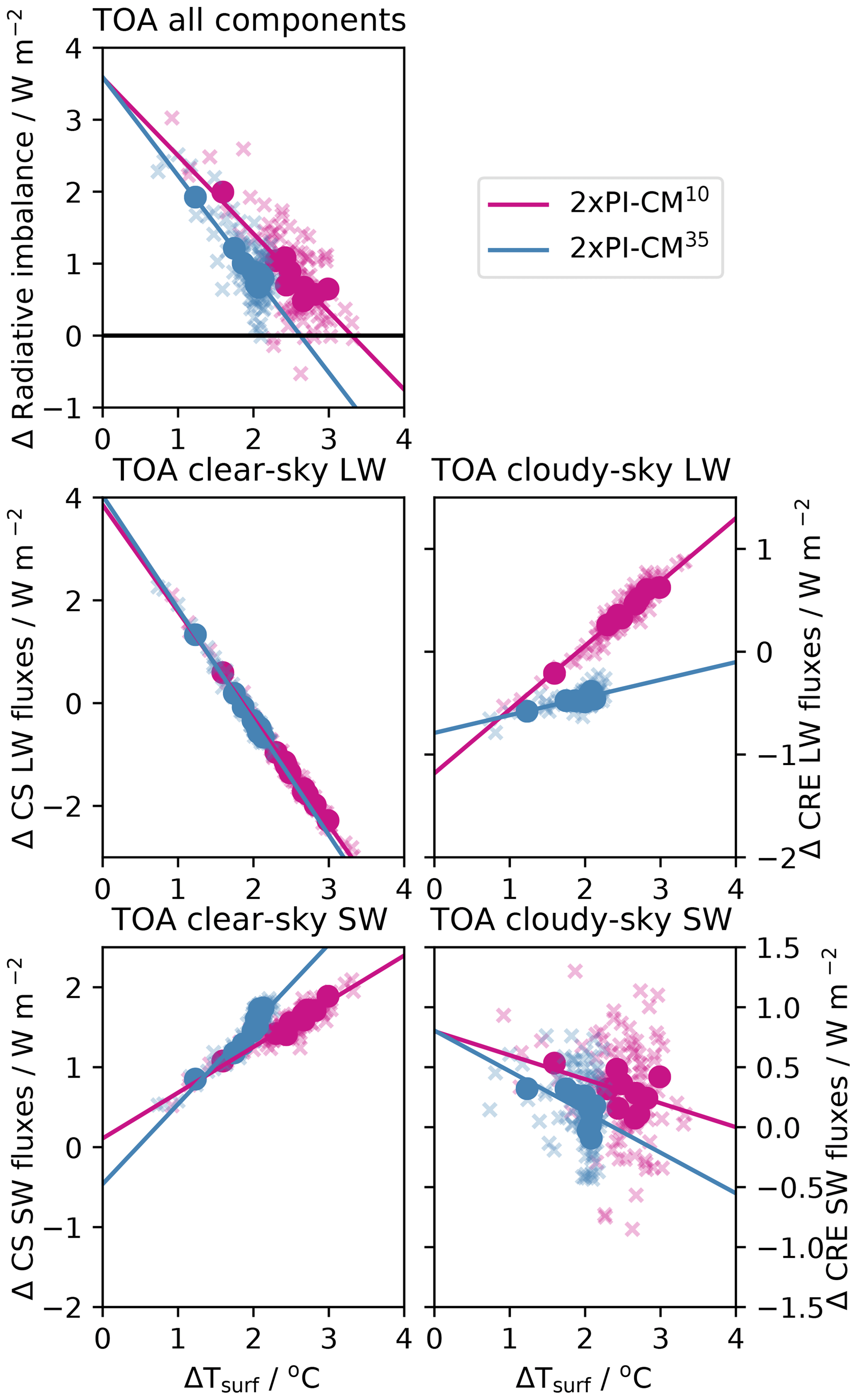
Figure 9 Gregory analysis of HadCM3-BL: regression of top-of-atmosphere radiative imbalance against surface air temperature change (solid lines) for the first 100 years of 2 × PI-CM¹⁰ (pink) and 2 × PI-CM³⁵ (blue) cases. Annual averages are indicated by crosses and decadal averages are indicated by filled circles. The regression was performed on the decadal averages.

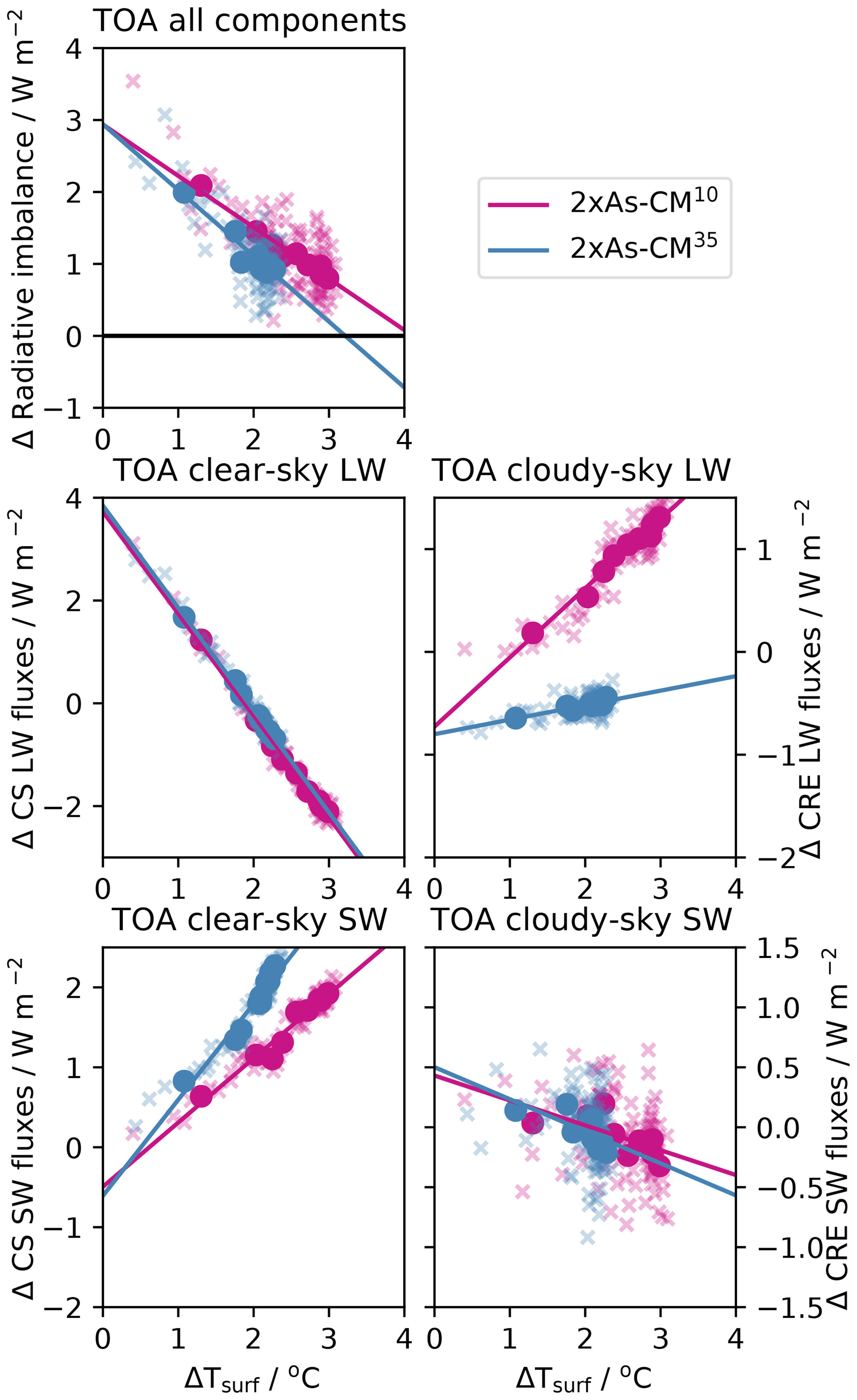
Figure 10 Gregory analysis of HadCM3-BL: regression of top-of-atmosphere radiative imbalance against surface air temperature change (solid lines) for the first 100 years of 2 × As-CM¹⁰ (pink) and 2 × As-CM³⁵ (blue) cases. Annual averages are indicated by crosses and decadal averages are indicated by filled circles. The regression was performed on the decadal averages.

3.3 Climate sensitivity

Here, we investigate the impact of oxygen variability on climate sensitivity. The HadGEM3-AO and HadCM3-BL results suggest that increasing CO₂ content leads to a reduction in the surface temperature change on increasing pO₂ (compare 4 × PI-GEM and PI-GEM in Fig. 4). For reference, HadGEM3 has a climate sensitivity of +3.6 ^∘C (Nowack et al., 2014), while HadCM3 has a climate sensitivity of +3.1 ^∘C (Johns et al., 2006). From the 4 × PI-GEM and PI-GEM experiments, a reduction in climate sensitivity of 0.65 ^∘C can be inferred based on the changes in surface temperatures. For HadCM3, CO₂-doubling experiments were performed, and a regression of the change in top-of-atmosphere radiative imbalance against change in surface temperature following Gregory et al. (2004) (see also Sect. 2.4) is shown in Fig. 9. The PI-CM³⁵ climate state has a smaller ECS than PI-CM¹⁰ by 0.7 ^∘C. While the changes in total radiative forcing F are very similar, ξ is less negative (−1.08 vs. −1.37 $\mathrm{W}{\mathrm{m}}^{-\mathrm{2}}{}^{\circ }{\mathrm{C}}^{-\mathrm{1}}$) at low pO₂. The decomposition of these changes into their longwave and shortwave components, clear-sky and cloudy-sky components is also shown in Fig. 9. The clear-sky longwave radiative flux changes are slightly higher in 2 × PI-CM³⁵ (4.0 W m⁻²) than 2 × PI-CM¹⁰ (3.8 W m⁻²) as would be expected due to the pressure broadening of CO₂. The clear driver for the less negative ξ value are from the longwave cloud radiative effect changes, which is much steeper for 2 × PI-CM¹⁰ (+0.62 $\mathrm{W}{\mathrm{m}}^{-\mathrm{2}}{}^{\circ }{\mathrm{C}}^{-\mathrm{1}}$) than 2 × PI-CM³⁵ (+0.17 $\mathrm{W}{\mathrm{m}}^{-\mathrm{2}}{}^{\circ }{\mathrm{C}}^{-\mathrm{1}}$). This is somewhat offset by stronger clear-sky shortwave radiative feedbacks in 2 × PI-CM³⁵ (+1.00 $\mathrm{W}{\mathrm{m}}^{-\mathrm{2}}{}^{\circ }{\mathrm{C}}^{-\mathrm{1}}$) than 2 × PI-CM¹⁰ (+0.57 $\mathrm{W}{\mathrm{m}}^{-\mathrm{2}}{}^{\circ }{\mathrm{C}}^{-\mathrm{1}}$). This highlights the important role that cloud radiative feedbacks play in determining the climate sensitivity.

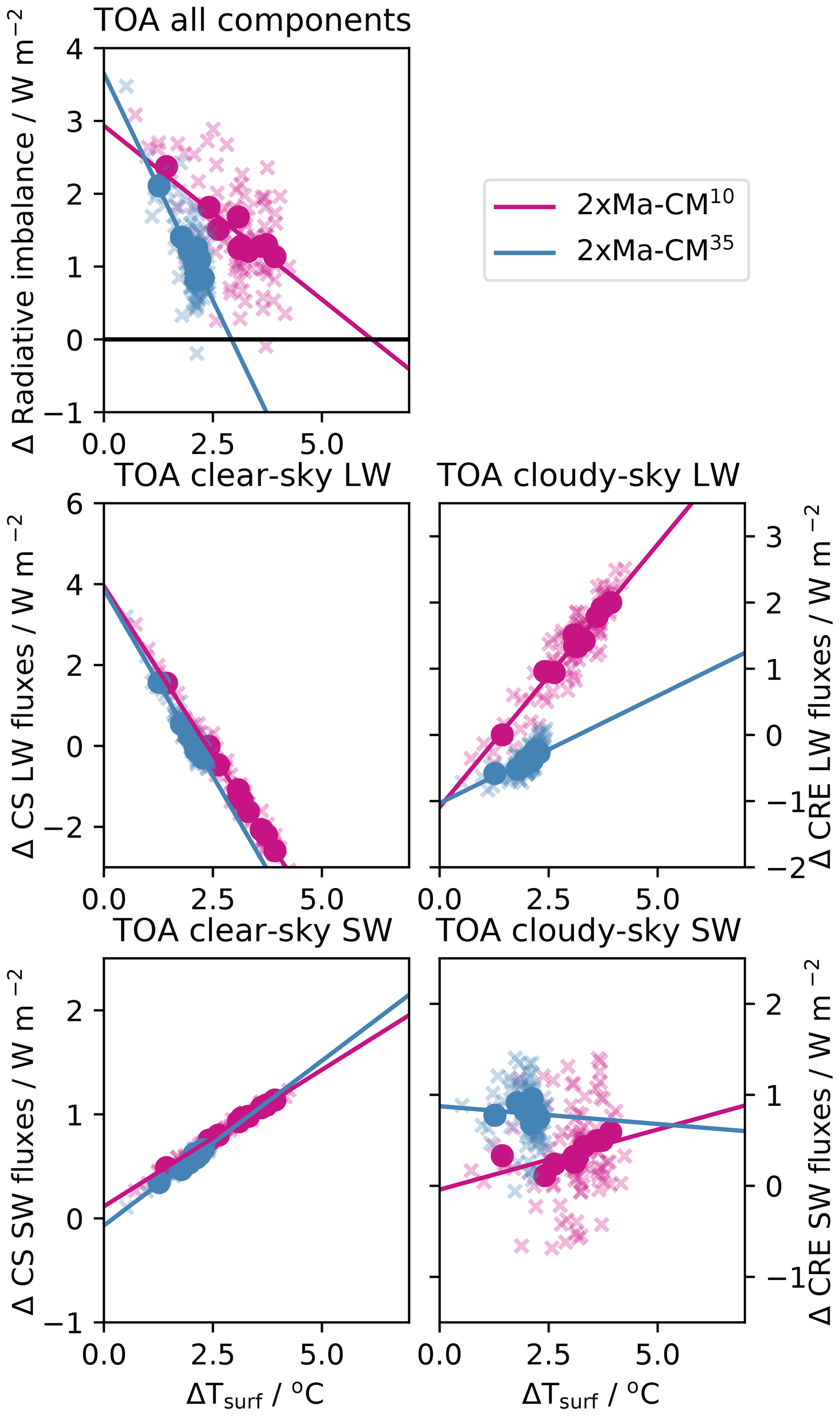
Figure 11 Gregory analysis of HadCM3-BL: regression of top-of-atmosphere radiative imbalance against surface air temperature change (solid lines) for the first 100 years of 2 × Ma-CM¹⁰ (pink) and 2 × Ma-CM³⁵ (blue) cases. Annual averages are indicated by crosses and decadal averages are indicated by filled circles. The regression was performed on the decadal averages.

An increase in ECS appears to be robust across the HadCM3-BL experiments. For As-CM, ECS is 0.8 ^∘C lower at 35 % O₂ than 10 % O₂ (Fig. 10). For Ma-CM, this value is much larger. A 3.3 ^∘C reduction in ECS is simulated, which is also driven by the longwave cloud radiative effects in conjunction with a weaker clear-sky shortwave radiative effect which tended to cool the low pO₂ (Fig. 11). Unlike the clear-sky shortwave effects, the longwave cloud radiative effects seem consistent across the three experiments. It should be noted that attempts were made to simulate 2× experiments for the Wuchiapingian; however, what would have been the 2 × Wu-CM¹⁰, in the nomenclature used here, was numerically unstable.

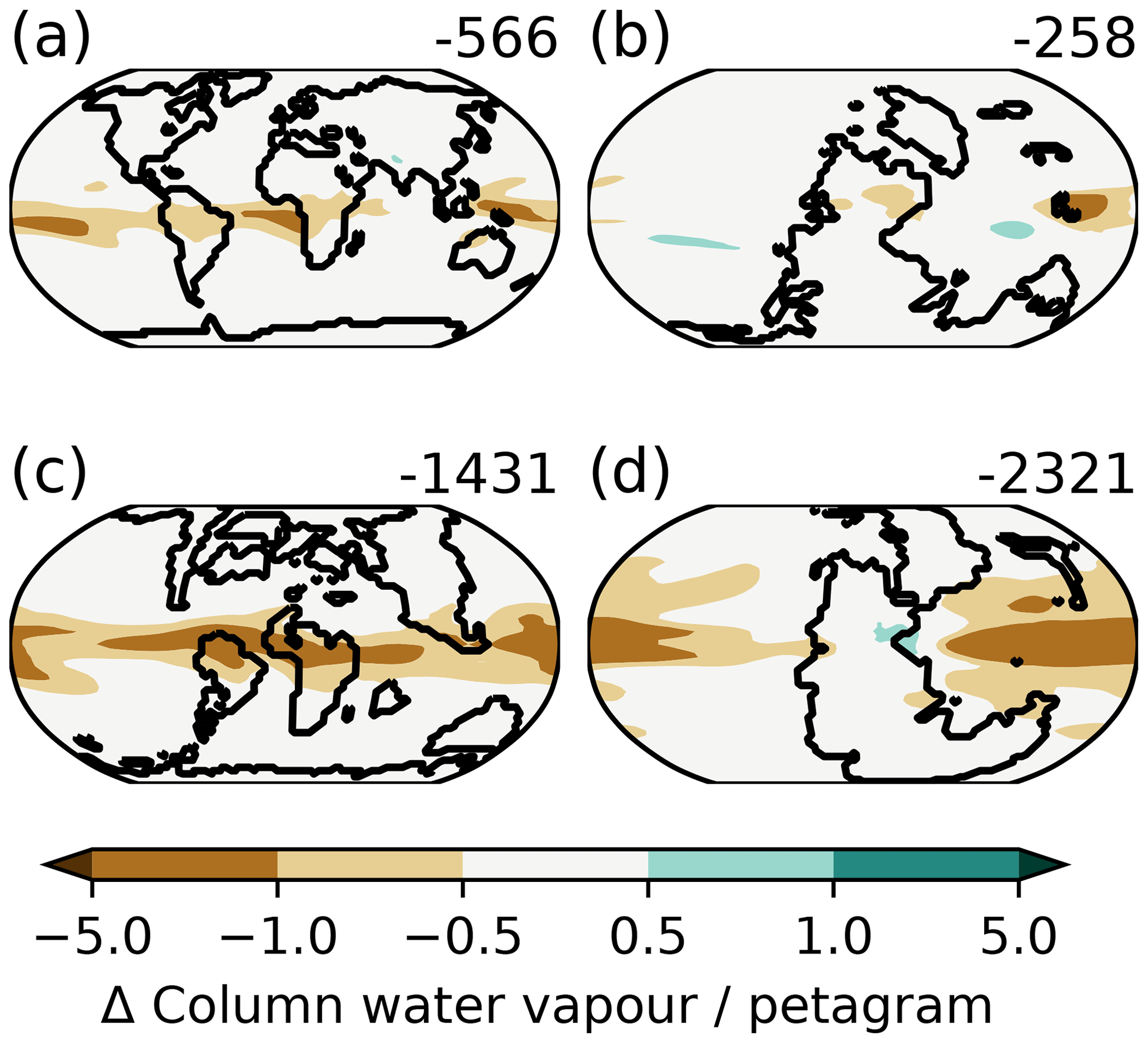
Figure 12 Change in column water vapour in (a) PI-CM${}_{\mathrm{10}}^{\mathrm{35}}$, (b) As-CM${}_{\mathrm{10}}^{\mathrm{35}}$, (c) Ma-CM${}_{\mathrm{10}}^{\mathrm{35}}$ and (d) Wu-CM${}_{\mathrm{10}}^{\mathrm{35}}$. Global sum values (petagrams) are offset to the top right of each plot. Note the atmospheric drying at high pO₂ is enhanced in the warmer climate states of the Wuchiapingian and Maastrichtian and more subdued in the cooler climate states of the Asselian and Holocene.

The increase in climate sensitivity appears to be linked to the reduction in temperature anomaly in a warmer climate state. We propose that this is due to more vigorous convection at low pO₂ (Goldblatt et al., 2009), leading to an atmospheric moistening (Fig. 12) which causes warming analogously to Rose and Ferreira (2013). This is consistent with the increases in climate sensitivity observed – in a warmer climate the atmosphere can hold more water vapour, so any changes to water vapour will be amplified in their impacts on the radiative budget of the atmosphere. This water vapour feedback is also consistent with the weaker clear-sky shortwave radiative effect observed in 2 × Ma-CM and the temperature response observed in the Wuchiapingian simulations.

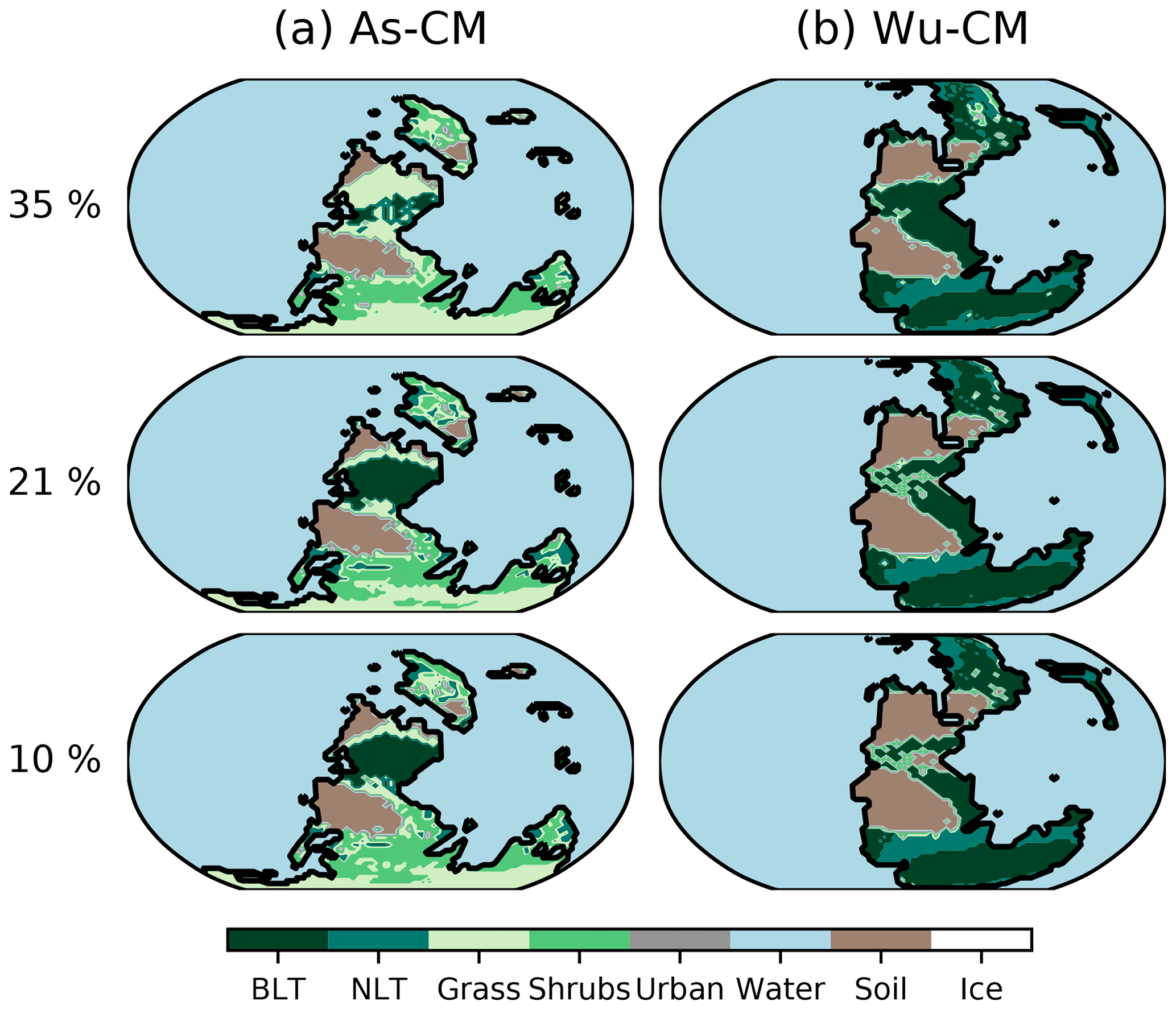
Figure 13 Dominant surface type for each oxygen level simulation for (a) As-CM and (b) Wu-CM. BLT: broadleaf tree; NLT: needleleaf tree.

3.4 Response of Permian vegetation to pO₂

Changes in pO₂ and surface temperatures have the potential to impact the terrestrial carbon cycle by altering the competition between the oxidative and photosynthetic metabolic pathways for RuBisCO. Beerling and Berner (2000) simulated significant changes to vegetation productivity in the Permian due to changes in oxygen content. The modelled changes to vegetation in the final 50 years of the Asselian and Wuchiapingian experiments are investigated. Focusing on changes to vegetation across the Permian, the dominant vegetation fractions for As-CM³⁵, As-CM¹⁰, Wu-CM³⁵ and Wu-CM¹⁰ are shown in Fig. 13. For low pCO₂ in the Asselian, increasing pO₂ leads to a reduction in the extent of broadleaf trees and greater proliferation of grasses and shrubs. This would be consistent with increases in photorespiration at high pO₂. The reverse is true in the Wuchiapingian simulations with increases in the extent of tropical broadleaf forests. It should be noted that the simulation of plant functional types is carefully tuned to present-day vegetation which was likely considerably different in the past. Therefore, caution should be exercised when extrapolating to past vegetation changes.

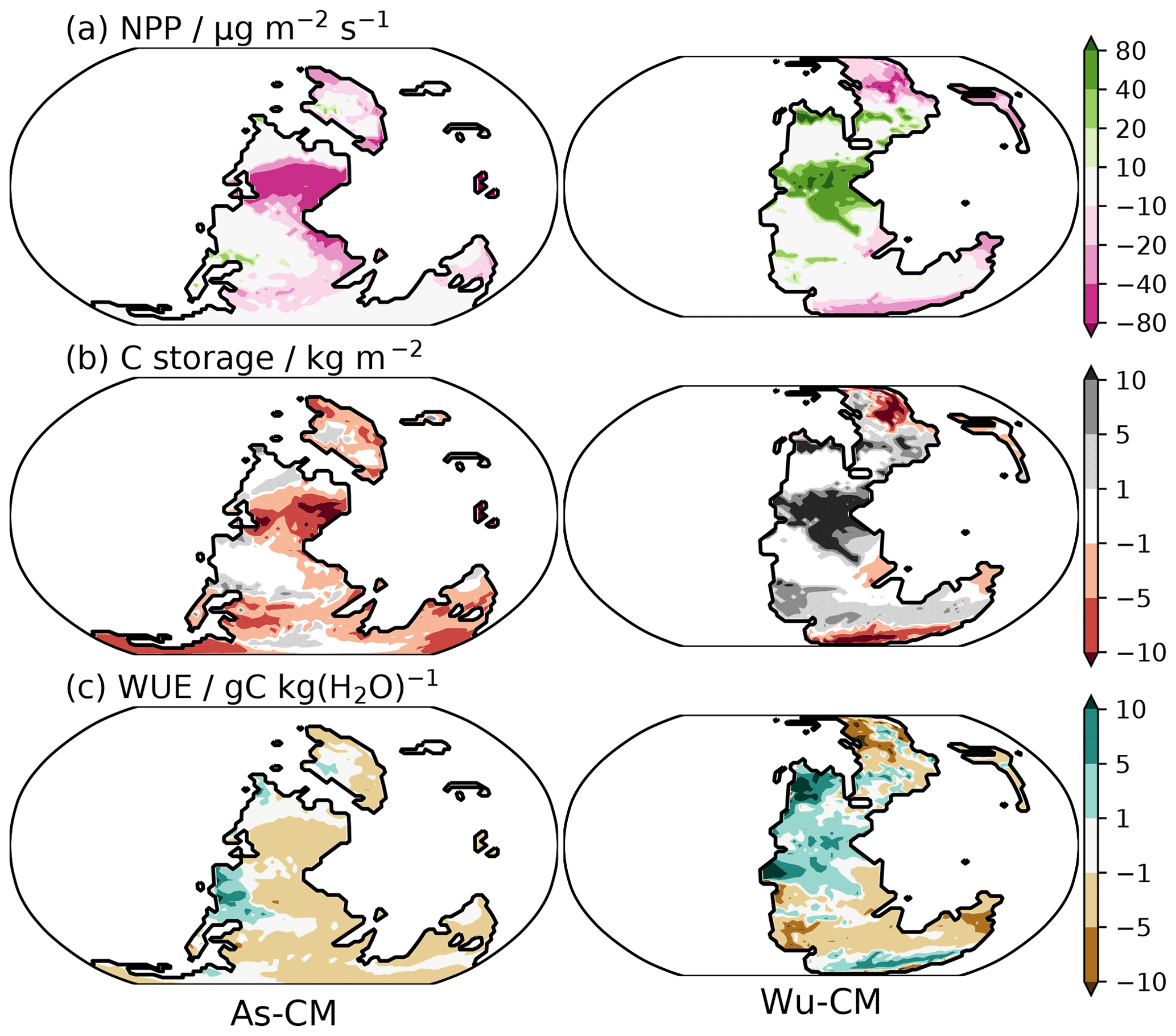
Figure 14 As-CM${}_{\mathrm{10}}^{\mathrm{35}}$ (left) and Wu-CM${}_{\mathrm{10}}^{\mathrm{35}}$ (right) anomalies for (a) net primary productivity, (b) total carbon storage and (c) water use efficiency.

Figure 14a shows the change in net primary productivity (NPP) for As-CM${}_{\mathrm{10}}^{\mathrm{35}}$ and Wu-CM${}_{\mathrm{10}}^{\mathrm{35}}$. The Asselian simulations shows a large reduction in net primary productivity (NPP) as pO₂ is increased (Fig. 14a, −59 Pg C yr⁻¹), while the reverse is true in the Wuchiapingian simulations (+33 Pg C yr⁻¹). At low pCO₂, it is expected that competition for RuBisCO will be won out by O₂ and therefore that rates of photorespiration should lead to a decline in photosynthesis. This is reflected in the gross primary productivity (GPP, −34 %) and NPP (−52 %) response for the Asselian. During the Wuchiapingian, there may be sufficient CO₂ that competition is much less sensitive to the pO₂ so changes to NPP are much less significant. In fact, NPP is increased by 14 % (GPP +18 %). Tropical water use efficiency is also higher in Wu-CM³⁵ (Fig. 14c), which suggests that water economy of plants could alter to adapt to a higher pO₂ (Beerling and Berner, 2000).

These net primary productivity changes are reflected in the total carbon storage (Fig. 14b) which is lower as pO₂ is increased in As-CM (−338 Pg C) and higher as pO₂ is increased in Wu-CM (+379 Pg C). This is dominated by changes in the tropics (in agreement with Beerling and Berner, 2000), where broadleaf trees cover more area in Wu-CM³⁵. Cooler terrestrial tropical temperatures, particularly in the warm months (Fig. 4e), reduce the pO₂ inhibition of RuBisCO and reduce the rate of respiration by vegetation and soils (Long, 1991; Beerling and Berner, 2000).

As these simulations are fully coupled and changes to oxygen content affect temperatures, radiation and precipitation, it is challenging to explore all the possible contributions to differences between these results and the more idealised Beerling and Berner (2000) simulations. However, there is general agreement that changes occur in the signs of the response of NPP and total carbon storage. This supports the conclusions of Beerling and Berner (2000) that high pO₂ in the early Permian may have played an important role in the evolution of plants. Note that while the atmosphere and vegetation are coupled in the physical sense, the carbon cycle is not interactive (atmospheric CO₂ is fixed), so determining the impacts of atmospheric pO₂ on the carbon cycle remains an outstanding problem.

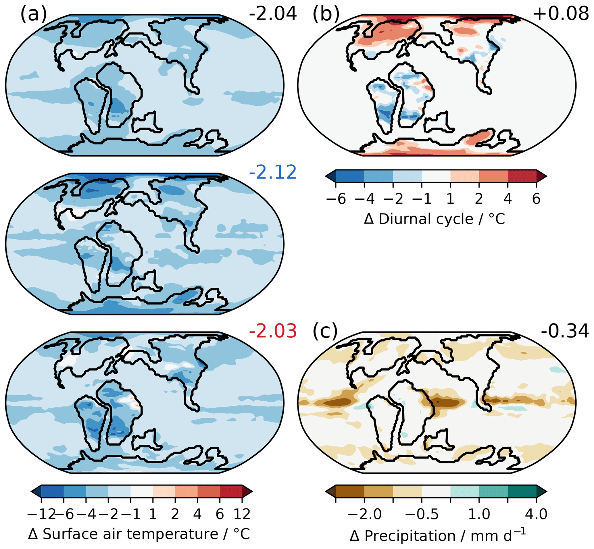
Figure 15 The 21 %–10 % O₂ anomalies for Poulsen et al. (2015) simulations. (a) Annual-mean, cold-month mean and warm-month mean surface air temperature difference. (b) Change to diurnal cycle and (c) annual-mean precipitation (mm d⁻¹).

Figure 16 1-D energy balance decomposition analogous to Fig. 7 for the 21 %–10 % O₂ Poulsen et al. (2015) simulations.

4 Discussion

Through its impact on atmospheric mass, oxygen content has the capacity to alter the radiative budget of the atmosphere and therefore has implications for the Earth's climate. These simulations suggest that the interactions between radiative and dynamical feedbacks lead to some consistent climatic changes in HadCM3-BL with increasing pO₂:

• reduction in the seasonal cycle in surface air temperature,

• reduction in Equator-to-pole temperature gradient and

• reduction in global precipitation.

HadCM3-BL simulates a reduced equilibrium climate sensitivity mainly due to changes in longwave cloud feedbacks. HadGEM3-AO results also support a reduced sensitivity to CO₂ content at high pO₂. The pre-industrial Holocene results are supported by 1-D radiative convective simulations (Payne et al., 2016), 2-D model simulations (Chemke et al., 2016) and slab ocean 3-D model simulations of the Archean (Charnay et al., 2013). This raises a discrepancy with the Poulsen et al. (2015) study, which simulated a reduction in global-mean surface temperature when increasing oxygen content in the GENESIS model. Figure 15a shows the surface air temperature change between the 10 % and 21 % Cenomanian (100.5–93.9 Ma) simulations from the Poulsen et al. (2015) study. These show a −2.04 ^∘C change in the annual mean. To understand the mechanisms behind this, we performed the 1-D energy balance decomposition on the Poulsen et al. (2015) Cenomanian 21 %–10 % model output. The results are shown in Fig. 16. This shows that the cloudy-sky contribution to the temperature change dominates the climate response, contributing −1.45 ^∘C. However, the clear-sky contribution is also negative (−0.60 ^∘C), including both clear-sky emissivity (−0.58 ^∘C) and clear-sky albedo (−0.11 ^∘C). This appears to support the argument that tropical cloud feedbacks explain the discrepancy between the Poulsen et al. (2015) simulations and results of 1-D radiative convective models (Goldblatt, 2016); however, this cannot be the only factor. An increase in pressure broadening of absorption lines would be expected to lead to a positive contribution from the clear-sky emissivity. This suggests that cloud feedbacks alone cannot explain the discrepancy and that the implementation of pressure broadening may play a role in the anomalous Poulsen et al. (2015) response. In addition, changes to the seasonal cycle (Fig. 15a) simulated by Poulsen et al. (2015) are also inconsistent with the HadGEM-AO and HadCM3-BL results, in which all simulations led to a reduced seasonal cycle as pO₂ increases. The Poulsen et al. (2015) Cenomanian simulations actually simulates a larger seasonal cycle at high pO₂, which is challenging to reconcile with the radiative and physical processes. Note that the Poulsen et al. (2015) simulations were for an earlier Cretaceous period (Cenomanian) than those performed in HadCM3-BL (Maastrichtian); however, the continental configurations and the global-mean temperatures are reasonably similar (22.2 ^∘C in HadCM3-BL vs. 20.5 ^∘C in Poulsen et al., 2015).

The simulations presented in here suggest that perturbations to the wind-driven ocean circulation by increasing atmospheric mass lead to warmer temperatures, particularly at high latitudes. The magnitude of the results varies depending on the precise continental configuration and background climate state. Gyre circulations vary between the pre-industrial and the Maastrichtian and Asselian case studies. Given the importance of the wind-driven ocean circulation response, this suggests that a 3-D representation of ocean circulation is necessary in order to capture the temperature response to atmospheric mass changes. It should be noted, however, that Charnay et al. (2013) simulated higher surface temperatures for the early Earth at high atmospheric mass with a slab ocean model.

The use of 3-D oceans is now widespread in the palaeoclimate community; however, this is not widely used in the exoplanet/early Earth community (e.g. Kilic et al., 2017) and for early Earth studies such as the Archean (e.g. Charnay et al., 2013). While boundary conditions for these studies are sparse or in some cases non-existent the additional uncertainty associated with using a slab ocean should be considered. AOGCM studies remain the best way to assess the complex coupling between potentially competing radiative and dynamical effects.

One criticism of high oxygen variability in the Phanerozoic is the possibility of runaway fire at high oxygen content (Watson et al., 1978). While subsequent experiments have put this in doubt (Wildman et al., 2004), fire is undoubtedly a negative feedback on oxygen content. However, the cooling of warmest-month temperatures over tropical and midlatitude continents in Wu-CM³⁵ may provide somewhat of a protective mechanism against runaway fire regimes taking hold. Lightning is a major cause of palaeofire (Scott and Jones, 1994), so the reduction in convection at high pO₂ would also lead to fewer lightning strikes, which would reduce fire initiation. In addition, higher fire risk could have favoured the evolution and spread of more fire-resistant species (Robinson, 1990).

The simulations of Permian climate (As-CM and Wu-CM) also suggest a strong role for pO₂ variability in the terrestrial carbon cycle. However, there are many limitations to the modelling approach employed here. The plant functional types employed here are the same as those for the present day. In particular, C₄ photosynthesis likely evolved in the Oligocene (Sage, 2004), although there is evidence of vegetation which causes C₄-like fractionation in the Mississippian, suggesting different vegetation adaptations operating in the past (Jones, 1994). In addition, angiosperms did not evolve until the Cretaceous, so gymnosperms such as cycads were more widespread in the Permian (Taylor et al., 2009). TRIFFID and other dynamic plant models were not developed with these changes in plant types in mind, so simulating past vegetation changes is still a considerable challenge. However, scientific understanding of the role of plants in the climate in the Paleozoic is still immature. While early evidence suggested that late Paleozoic vegetation was unproductive based on analysis of the closest modern relatives, this perspective is increasingly being challenged (Wilson et al., 2017). Other approaches such as trait-based methods (Van Bodegom et al., 2012; Porada et al., 2016) may be able to achieve more insights into the role of pO₂ in the Earth system. We also have not accounted for changes to the ocean carbon cycle. A biogeochemical model study suggests that pervasive oceanic anoxia and euxinia only occur below an oxygen level of around 10 % (Ozaki and Tajika, 2013), which may be below the fire threshold (Belcher et al., 2010) and therefore not of relevance to many periods in the Phanerozoic. However, the extent of oceanic anoxic events may be sensitive to atmospheric pO₂ (Clarkson et al., 2018).

Figure 17 (a) Reconstructed CO₂ (doubling from Pleistocene values, blue) and O₂ content (red) and 95 % confidence intervals (shading) from Royer et al. (2014) Geocarb simulations. (b) GMST reconstructed using Geocarb pCO₂ and climate sensitivity values (purple) and the uncertainty in GMST from pCO₂ uncertainty (purple shading). GMST reconstructed, accounting for pO₂ according to Poulsen et al. (2015) global-mean temperature sensitivities (solid orange) and the uncertainty due to Geocarb pO₂ (dashed orange).

Given the small changes in global-mean surface temperature (GMST, 1.5 ^∘C maximum) compared to ECS (∼3 ^∘C), this raises the question of how much pO₂ variability contributes to uncertainty in Phanerozoic surface temperature even with such large uncertainties in pO₂ reconstructions. Figure 17 shows reconstructed Phanerozoic surface temperatures based on CO₂ content and climate sensitivity from the Geocarb model (purple; Royer et al., 2014). The uncertainty associated with the 95 % confidence interval in simulated pCO₂ is also indicated (purple shading). Analysis of the Poulsen et al. (2015) simulations suggests a global-mean surface temperature reduction of 0.21 ^∘C per percentage increase in O₂. Accounting for the pO₂ simulated by Royer et al. (2014) leads to a mean absolute difference in global-mean surface temperature of 0.80 ^∘C and maximum absolute difference of 2.59 ^∘C (Fig. 17 orange line). The largest deviations from the Geocarb values occur during the largest deviations from present atmospheric levels of O₂ during the Permian. However, pO₂ contributes little to the uncertainty in reconstruction of global-mean surface temperature compared to pCO₂ (Fig. 17, dashed orange lines), even if the temperature changes simulated by Poulsen et al. (2015) are reasonable. The HadGEM3-AO and HadCM3-BL simulations show even less sensitivity of global-mean surface temperature to pO₂ changes, which suggests this is likely an overestimate.

pO₂ therefore remains a secondary contribution to climatic variability in the Phanerozoic in agreement with Payne et al. (2016) but is most likely to be important during the Permian. The Artinskian (early Permian, 283.5–290.1 Ma) is associated with a rapid increase in CO₂ content from ∼500 to ∼3500 ppmv, which is associated with considerable restructuring of tropical vegetation (Montañez et al., 2007). The results in this study suggest that pO₂ variability could have modulated the climate and terrestrial vegetation response to this increase in CO₂ content. Feulner (2017) suggested that Earth was close to entering a Snowball Earth in the late Carboniferous, when pO₂ was higher than today. We hypothesise that the carbon cycle and physical climate feedbacks described in this paper would strongly mitigate against this. If pCO₂ and pO₂ are intimately linked such that cooler climates tends to increase pO₂, this would suggest that pO₂ responses have helped to prevent Snowball Earth initiation in the Phanerozoic.

5 Conclusions

The numerical simulations performed in this study reconcile the surface temperature response to oxygen content changes across the hierarchy of model complexity:

• Under pre-industrial Holocene conditions, increasing atmospheric pO₂ leads to an increase in global-mean surface temperature in agreement with 1-D radiative–convective model simulations. This increase is greater in the cold-month mean than in the warm-month mean. The Equator-to-pole temperature gradient is reduced, particularly in the cold-month mean, consistent with a stronger greenhouse effect at high atmospheric pressure.

• Lower incident surface shortwave radiation leads to a slowdown of the hydrological cycle. Precipitation decreases globally under high pO₂, with regional variations.

• The climate sensitivity is lower at high pO₂, particularly in the Maastrichtian. This appears to reconcile the results of the 1-D and 3-D modelling approaches.

• The climate response simulated by Poulsen et al. (2015) is inconsistent with the radiative changes when considering a 1-D energy balance model decomposition of the surface temperature changes. Tropical cloud feedbacks alone were not sufficient to explain the discrepancy.

• The climate response to oxygen content variability is state-dependent, so it should be considered on a case-by-case basis. However, the changes are relatively small compared to the role of CO₂ in the Phanerozoic (Royer et al., 2014).