the Creative Commons Attribution 4.0 License.
the Creative Commons Attribution 4.0 License.
 | 27 Mar 2026
On the computation of several “insolation” quantities relevant to climatology or planetology
Didier Paillard
There are many possible “insolation” quantities. When looking for some astronomical forcing, geologists, paleoclimatologists and climate modellers are often limited by the available software or web sites that compute or distribute some specific time series, often with a quite limited documentation. Furthermore, the astronomical forcing has several subtleties that some people might not be aware of, especially the key difficulty of defining a calendar. This paper aims therefore at presenting and documenting a rather complete python library designed to compute many astronomical and insolation quantities relevant to climate: standard ones like for instance daily insolation; less classical ones like integrated insolation over time or over space (or both); but also new quantities that are sometimes discussed in the literature on a qualitative basis, like the semi-precessional forcing at low latitudes, something which involves computing minima and maxima of the solar forcing over the year, a surprising complex endeavour when looking at generic planetary situations with arbitrary eccentricity or obliquity. Overall, the aim is here to provide not only a useful toolbox for scientists, but also a pedagogical introduction of some subtle difficulties for students. This is done using the widely used computer language python so that the code is easy to understand, to reuse or modify for various different contexts.
- Article
(4347 KB) - Full-text XML
- BibTeX
- EndNote


The role of orbital parameters on Earth's climate has been discussed since the discovery of glacial cycles in the 19th century. It can be easily shown that the three astronomical parameters relevant for computing the incoming solar radiation are the eccentricity (e) of the Earth's orbit, the tilt or obliquity (ε) of the Earth's axis with respect to the orbital plane, and the climatic precession angle (ϖ), which represents the relative angular position of the seasons with respect to the perihelion (see for instance: Paillard, 2010; Berger et al., 1993). From these three numbers, it is possible to compute many “insolation” quantities, for instance, at different locations, different seasons, integrated over some time or spatial ranges, eventually above some threshold, or when they reach some maximum or minimum value. Indeed, for most paleoclimatic questions, we do not have a full deterministic understanding of the processes involved and it might be relevant to choose one or the other “insolation” quantity as a first approximation of the corresponding full actual astronomical forcing.
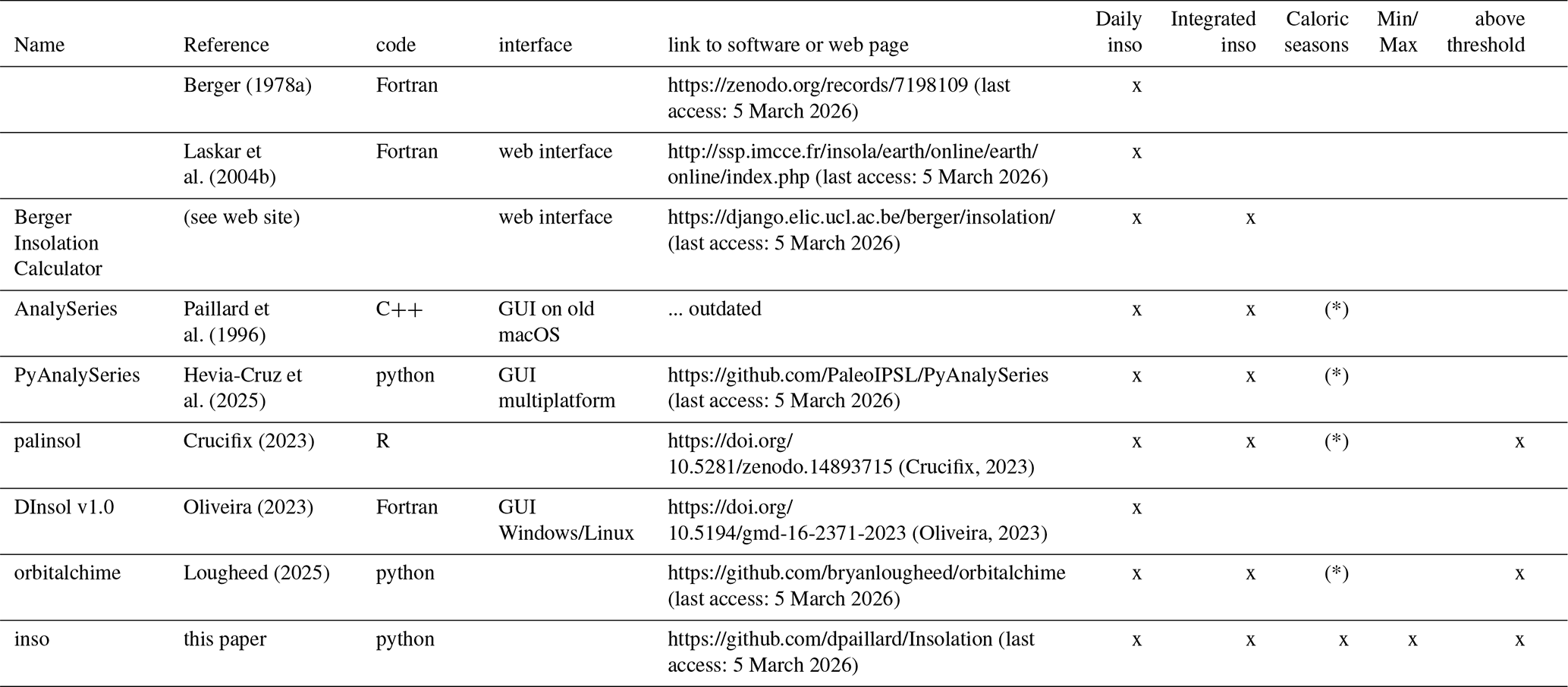
The term “insolation” usually refers to the solar irradiance (measured in W m−2), ie. the power received by the Earth, per unit area, at the top of the atmosphere. But we are interested here in many possible different “flavours” of this quantity, through averaging over the day, over some season, over some spatial area, or by taking some specific extrema. In order to avoid confusion, we will use the term “insolation” between quotes in a loose sense, while using much more specific vocabulary and notation when necessary. Depending on the needs, the environments, the preferred platforms or languages of the user, several software packages are available. Below (in Table 1) is a small and not exhaustive list of some possible options to compute easily such insolation quantities.
Table 1A short, non-exhaustive list of available software for insolation computations. The (*) symbol in the “caloric season” column is meant to highlight that the software might not be able to compute the insolation over caloric seasons for all possible orbital configurations (in particular at low-latitudes with multiple maxima) but was designed mostly for the ice age problem (high latitudes and Earth-like parameters) as discussed in the main text (see for instance Fig. 10).
Concerning the growth and decay of the large Northern hemisphere ice sheets in the context of Quaternary glaciations, several different suggestions have been put forward (see Paillard, 2015, for a review). Since the 19th century, it was obvious that a global mean insolation was not relevant to climate, and for this reason, astronomers and physicists were not in favour of any astronomical theory of climate. But since the key phenomenon involves ice-sheets at high northern latitude, it was nevertheless suggested that a much more relevant quantity should be some high northern latitude insolation forcing. If earlier attempts were focussed on winter insolation, Milankovitch (1941) emphasized that ice-sheet evolution should be linked mostly to summer temperatures and he therefore advocated the use of some summer high northern latitude insolation forcing. More precisely, he defined the “caloric summer” as being the half-year during which the insolation, for any specific day, is larger that the insolation during the other half, the “caloric winter”. He then computed manually, using series expansions, the corresponding “insolation” quantities at different latitudes over the last 500 kyr. Since the 1970's, a more popular definition of “summer insolation” is the daily insolation at some specific date: either at the summer solstice which is well-defined astronomically or sometimes at mid-july or some other specific date which might critically depend on a choice of a calendar (Berger, 1978a). Still, the use of the averaged insolation over some period of the year has always been considered useful (Loutre et al., 2004). More recently, it was also suggested that computing the sum of incoming solar radiation over some given threshold could be more relevant to the (threshold) phenomenon of ice freezing/melting (Huybers, 2006).
A mistake frequently made by students or non-specialists is to compute the average or integrated insolation over some season, or any other time period, by simply computing the mean of daily insolation values within the interval. In most cases, the result is not what is intended. Indeed, it is critical to account for the varying duration of seasons when the precession parameter changes, something which requires dedicated methods and softwares (see Table 1). This varying speed of the Earth on its orbit corresponds in fact to the actual precessional forcing, since it can be easily demonstrated that the integrated amount of energy received between two orbital location does not depend on precession. A rather similar mistake is to compute, for instance, some northern hemisphere autumnal (September) insolation using the daily insolation values exactly a half-year after the NH-spring (March) equinox, something that is sometimes done implicitly by some software. In both cases, these mistakes arise from the difficulty to define a calendar when the precession parameter is widely different from today. Indeed, the usual implicit choice is to define 21 March as the NH-spring equinox, while the number of days within each astronomical season varies significantly. Astronomers use a less ambiguous vocabulary: they define the “true longitude” of the Earth as being the angular position with respect to the vernal point (NH-spring equinox) and the “mean longitude” of the Earth as the position it would have if the Earth's movement were regular: in other words, “mean longitude” stands for “time of the year”. Obviously climate models are using “time” or “mean longitude” in order to compute their radiative forcing. But when looking at paleoclimatic data, it usually makes more sense to use “true longitude” to better capture some specific orbital configuration.
Computing correctly integrals or averages of insolation, over some season or some time interval, is in fact what Milankovitch used as a definition of “caloric seasons” and it certainly still stands as a quite useful quantity to interpret paleoclimatic changes. But computing correctly spatial averages is also very useful and often disregarded. For instance, in climate models, a usual practice is to use “mid-point” values as a surrogate for average values. This is probably a reasonable approximation when the grid-size is “small enough”, but for lower resolution models, such an approximation can be widely different from the true average, with errors of a few percent (larger than the astronomical changes) or even several tens of percent at some specific locations and time. Instead, the correct integral formulas are quite simple as I will show below and they could be easily implemented in models.
Beyond the question of Quaternary cycles, there are many other climatic questions that are not directly linked to northern hemisphere summer forcing. For instance, at low latitudes the precessional forcing is dominant and power spectra of paleoclimatic records often contain some semi-precessional component. It is very likely that this results from some climatic non-linearity and a corresponding amplification of the first harmonic of the precessional forcing. But it might also be possible, as suggested in some publications, that this semi-precessional component originates directly from the astronomical forcing (McIntyre and Molfino, 1996). It is therefore useful to provide “insolation” time-series showing such a component, the simplest candidate being the minimum or maximum values of daily averaged insolation. Indeed, within the tropics the seasonal insolation variations are small, but there are possibly two maxima and two minima. The largest maxima can occur either close to one equinox or the other, depending on precession. At some low-latitude locations the precessional astronomical forcing therefore induces a semi-precessional “insolation” forcing when looking at extremal values of insolation (Berger et al., 1997). But interestingly, this phenomenon may partly or entirely disappear when obliquity is sufficiently low and eccentricity sufficiently high, as we will demonstrate later in this paper. Besides, computing these extrema is also a step to compute precisely the insolation above some threshold, or over caloric seasons, for all possible astronomical situations. Overall, it turns out that the computation of minima and maxima of daily insolation at some given latitude for any possible value of obliquity and eccentricity is a non-trivial problem that will be fully examined below.
The software and mathematical formula presented here are quite generic and not restricted to Earth. Still, we are assuming that the rotation of the planet is much faster than its revolution around its star. In other words, we are assuming that the planet does not move on its orbit when computing values for some specific day. This is certainly valid for Earth, but also certainly not valid for planets whose rotation is tidally locked, like for instance Mercury. Using this assumption, a main focus of the paper will be to compute various seasonal insolation quantities for some given configuration of the three astronomical parameters (eccentricity e, obliquity ε, climatic precession angle ϖ).
2.1 Astronomical parameters
The library “astro.py” provides a useful unified interface to several astronomical solutions for the past and future parameters of the Earth: Berger (1978a), Laskar et al. (1993, 2004b, 2011), as well as the one used by Milankovitch in his early publications (1920): Stockwell-Pilgrim (1904). It thus provides the astronomical parameters required to compute the various different flavours of “insolation” described in the following. More specifically, the Berger (1978a) solution is a trigonometric approximation whose validity is quite restricted and should probably not be used beyond about one million years. Just as the Stockwell-Pilgrim (1904) or the Laskar et al. (1993) solutions, it is provided here mostly for historical reasons, in order to illustrate the influence of these various solutions on the results. The current reference solution is the Laskar et al. (2004b) one. It is available from 101 Myr in the past to 21 Myr in the future, though its validity is probably questionable beyond 40 or 50 Myr (see Laskar et al., 2004, 2011). The Laskar et al. (2011) solution provides only eccentricity values and cannot be used for insolation computations.
Orbital parameters of planet Mars are also available through the solutions Laskar et al. (2003, 2004a) and from 21 Myr BP to 10 Myr AP. Indeed, though the paper is mainly focussed on the Earth, the provided libraries can be used on any “fast rotating” planet, and can directly be used to study, for instance, past Martian climates.
2.2 Daily insolation
To discuss seasonality, we need to define the position of the Planet on its orbit: one possibility is to use the angular position, or true longitude λs usually measured from the NH-spring (or march) equinox; the other possibility, discussed in the next paragraph (Sect. 2.3), is to use the time of the year, though this requires some calendar. We will furthermore look at insolation quantities at different latitudes φ. In the following, we will most of the time integrate over the rotation of the Planet, which is measured by the hour angle H (with H=0 corresponding to noon). It can be shown that the instantaneous insolation WI is given by , where S is the solar constant (approximately 1365 W m−2 for the Earth), a is the Earth's orbit semi-major axis, r the Earth-Sun distance, and z is the solar zenith angle (angle between the Sun and the vertical). This can be written as (see for instance Berger, 1978a):
where δ is the declination of the Sun, given by sin δ=sin εsin λ.
More precisely, the instantaneous insolation WI is given by Eq. (1) only if it is positive, i.e. when the Sun is above the horizon. By solving WI=0 or cos z=0, we get the hour angle h of sunrise or sunset: when it exists, which means when . Otherwise, we have h=0 during the polar night and h=π during the polar day.
Obtaining the daily averaged insolation is rather straightforward:
In these formulae, the Earth-Sun distance r is given by the polar equation for an ellipse: , with v (the “true anomaly”) being the location of the Earth on its orbit with respect to the perihelion: (λ is the location of the Earth on its orbit with respect to the vernal point in a geocentric view, ϖ is the location of the perihelion with respect to the vernal point in an heliocentric view, therefore we need to add a half-turn π to account for the change of referential). This leads to:
It can be useful to provide a simple formula for h, valid even in polar regions. This can be achieved by defining:
and p=sin φsin δ (with sin δ=sin εsin λ).
Then we always have: , with s=0 during the polar day or polar night and .
The above formula for WD becomes:
The daily insolation WD is therefore the product of the solar constant S, with a factor linked to the Earth-Sun distance involving the eccentricity e and the Earth's location with respect to the perihelion (λ−ϖ), and with a third “geometric” term depending on φ and δ, in an entirely symmetric fashion, corresponding to the averaged zenith angle 〈cos z〉. More precisely, this last term is:
In other words, the daily insolation can be written as , where we clearly see that the “geometric” term depends both on the average height of the Sun above the horizon 〈cos z〉 and also on relative day length . The astronomical parameters (e, ε, ϖ) have different roles in the daily insolation: obliquity (ε) influences only this last geometric term while eccentricity and precession (e, ϖ) intervene only through the distance factor .
2.3 Calendar
As mentioned in the introduction, the definition of a calendar can be a source of difficulties. Indeed, our usual calendar is designed to follow the seasonal cycle and it seems natural to us that equinoxes occur near the 21 March and 21 September, and solstices near the 21 June and 21 December. But this approximately applies only for our current astronomical setting, with a slightly shorter winter (DJF = 90.25 d) and a slightly longer summer (JJA = 92 d) or 186.5 d between March equinox and September equinox, but 178.5 d between the September and March ones. This corresponds to Earth's perihelion being currently reached in winter (the Earth's movement being then faster), as well as to a rather small difference in season durations, in accordance with the current small eccentricity. But we should remind that we have two different ways to account for the seasonal move of the Earth on its orbit: either its true angular position – i.e. the “true longitude” λ already introduced in the preceding section – or the elapsed time from some reference position (usually arbitrarily taken as the NH-spring location) – i.e. the “mean longitude” L. Obviously, applying our current calendar to very different orbital configuration can lead to some serious misinterpretations and it is therefore critical to understand this key difficulty.
Applying Kepler's 2nd law, it is rather simple to translate the true angular position (true longitude λ) into the time needed to reach it (mean longitude). This conversion can be obtained more easily when measuring time and angle from the perihelion. The true angular position is then called the “true anomaly” v as already introduced above (with and the “time” from this perihelion position is called the “mean anomaly” measured in radians, with T=1 year. To be very precise, T should be one anomalistic year, i.e. the (averaged) time for the planet to travel from perihelion to perihelion. But for the Earth, the difference with our civil year (based on the tropical year) is very small. Kepler's 2nd law states that the line joining Earth and Sun sweeps equal areas of space during equal time. This can be written as:
Using the equation of the ellipse , we get:
Using the change of variables , we finally obtain the famous Kepler equation:
where E is traditionally called the “eccentric anomaly”.
To summarize, knowing the true longitude λ, we also know v and therefore also E. The corresponding mean anomaly, or “time” M (measured from the perihelion) is then directly given by Eq. (3). The mean longitude L (from the NH-spring equinox) can also be obtained by applying the same procedure to λ0=0 to obtain the mean anomaly of the reference point , the mean longitude being finally the difference between these two mean anomalies . More generally, we can compute in this way the time needed to move from one orbital position λ1 to another one λ2. The length of seasons may itself be a quantity of interest for paleoclimatic studies, as discussed in Berger et al. (2024). In the library, this corresponds to the routine “length_of_season”.
The reverse is also true: from the mean longitude L (or true time using a given calendar), we can compute the true longitude λ. First, like before, we need to compute the mean anomaly M0 of the reference point to obtain the mean anomaly , then solve the Kepler equation to get the “eccentric anomaly” E, then use the change of variable to obtain v, and finally deduce . This corresponds to the routine “trueLongitude”. For instance, climate models are based on differential equations, which means that they compute climate quantities as functions of elapsed time. Therefore, they need to use some specific calendar to represent “time” within the annual cycle, and then transform this time into a true orbital position λ. This is precisely what this routine is doing.
When computing the daily insolation at some specific “season” or “time of the year”, it is critical to understand the difference between “true longitude” (for example, the astronomical seasons) and “time elapsed since some reference point” (in the way our calendar is built). As shown in Fig. 1, this can make a huge difference. Traditionally, the “reference point” is the NH-spring equinox, which is associated to 21 March. Indeed, march was the first month of the year in the Julian calendar since spring is naturally associated with the beginning of the year. This (often implicit) convention means that the NH-autumn equinox can vary widely around 21 September (usually defined as being about half a year after 21 March), depending on precession.
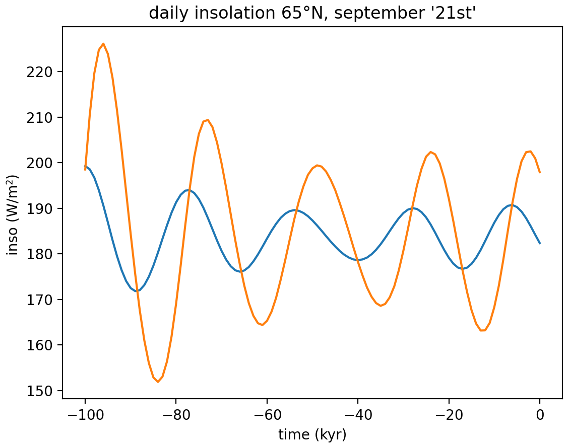
Figure 1Daily insolation at 65° N for “21 September”: In blue, it corresponds to the true (astronomical) september equinox, ie. true longitude λ=π. In orange, it corresponds to half a year after the reference point of the calendar (conventionally the spring equinox) ie. mean longitude L=π. As shown on this example, it is critical to understand the difference between “true longitude” and “time” (or “mean longitude”), since the amplitude and phase are very different between the two results.
3.1 Integrals between true longitudes
The daily insolation can be a good “proxy” for some phenomena, but it seems physically more relevant to integrate this forcing between two orbital locations that can be defined either by their true longitude or by some time interval. For instance, it might be interesting to define a northern hemisphere “summer” forcing by integrating the forcing between the spring and autumnal equinoxes: . This would give an energy (J m−2) received over a non-constant time interval as explained above. A better option would be to use the associated averaged insolation (W m−2), simply by dividing by the corresponding duration: In fact, Milankovitch used another possibility (Milankovitch, 1941; Berger, 1978b), which is to integrate the daily forcing over a fixed given duration, exactly half a year. More precisely, it is possible to find a threshold value such that the insolation exceeds it during half a year (the “caloric summer”) while remaining below it during the other half (the “caloric winter”) and to compute the corresponding integrated insolation over these two periods (J m−2), or equivalently the corresponding averaged insolation WCalS and WCalW (in W m−2) since the duration is by definition a constant (half a year). It is critical to note that WS and WCalS are in fact entirely different quantities as illustrated below on Fig. 2.
Though this definition is quite simple, the precise computation of WCalS is difficult in the generic case, in particular when there are several maxima or minima of insolation during the annual cycle. This will be discussed later on in details in Sects. 4 and 5 below. Still WCalS is most often used in the context of Quaternary climates and ice ages, for Earth-like situations at rather high latitudes. Then, the “caloric summer” is extremely close to the half-year time period centered at the summer solstice as will be shown later (see Fig. 10). For such situations, we can therefore compute a very good approximation of WCalS as . Similarly, we can also define the winter counterpart as .
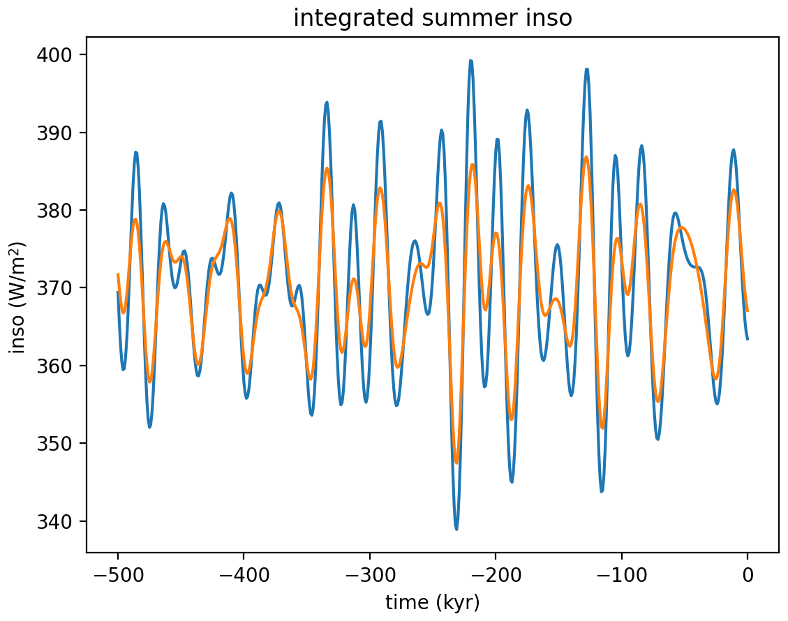
Figure 2Averaged NH-summer insolation defined in two different ways. In blue WS the insolation averaged between the march and the September equinoxes (between the true longitudes 0 and π). In orange WCalSSol (a very good approximation of WCalS) the insolation averaged over half a year centered at the summer solstice, ie. the “caloric summer” defined by Milankovitch. The blue curve contains much more precession and is quite similar to the summer solstice daily insolation. The mean “caloric summer” insolation contains relatively more obliquity.
But before providing formulas for these quantities, it is worth emphasizing that the integrals are “time” integrals. It is therefore not correct to add the daily insolation taken at some different positions nor to take the corresponding average. In contrast, it is necessary to perform some specific computation using suitable software packages (see Table 1). In other words, should not be confused with . Indeed, here again it is critical to account for the non-uniform motion of Earth on its orbit since is not constant. We need to use, once more, Kepler's second law . This gives:
With 〈cos z〉, this leads to:
Interestingly, for fixed values of (λ1,λ2) we can note that the climatic precession angle (ϖ) has entirely disappeared from this expression, since it is involved only in the term – but we still have obliquity (ε) in h〈cos z〉 and eccentricity (e) in the denominator. In other words, the amount of energy J12 received between two given true longitude (λ1,λ2) does not depend on precession. For , we do recover the precessional forcing, but only thanks to the division by the time interval (tAutumn−tSpring) since the conversion between true longitude and time depends on precession and eccentricity. In the caloric summer , the longitudes of the integration interval are not fixed, but depend themselves on precession. These two possible definitions of “summer” lead to significant differences as illustrated on Fig. 2. All these remarks demonstrate how the precessional forcing is intimately linked to the varying speed of Earth on its orbit and Kepler's 2nd law.
We can more generally define:
After some computation, we can express the results using elliptic integrals (e.g. Loutre et al., 2004; Berger et al., 2010):
where and , are the elliptic integrals (Legendre notation) of the 1st, 2nd and 3rd kind:
But the functions F(λk) and Π(λsin 2εk) are not always well-defined in our domain of interest and it is preferable to compute directly the sum defined by:
All these elliptic functions are evaluated using Carlson integrals, using the SciPy library (Virtanen et al., 2020), for efficiency and for larger domains of definitions (in particular when k>1). Finally, the time interval (t2−t1) can be computed as explained in the above section (using Δt = length_of_ season(trueLon1, trueLon2, e, pre)). This gives W12 in Eq. (4). The approximation of the “caloric summer” insolation WCalSSol can be obtained similarly by first computing the true longitudes and then using again Eq. (4).
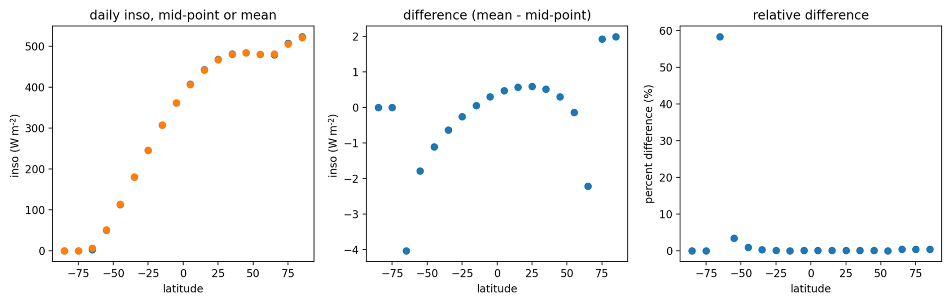
Figure 3Left: Present-day june solstice daily insolation on a latitude grid with a 10° resolution, using mid-point values (WD in blue) or computing the correct averaged values (〈WD〉AB in orange). Middle: The difference WD−〈WD〉AB can be as high as a few W m−2, comparable to some astronomically induced changes. Right: The relative error can be very high at latitudes near the polar night transition.
3.2 Integrals between latitudes
It can be also sometimes useful to integrate the daily averaged insolation between two different latitudes:
This can of course be done numerically, but there is a strong risk to obtain unreliable values near the discontinuities when sunrise or sunset appear or disappear. Furthermore, the corresponding analytical integrals are not difficult to obtain and are certainly more precise and reliable. I have not found such expressions in the literature and I think it could be useful to use them. This is for instance the case for low-resolution models: indeed, quite generally, models use the “mid-grid point” values instead of a numerical computation as an approximation for the true average. This might lead to quite significant errors, as show on the example below (Fig. 3). More generally, when comparing models that have been run at different resolutions, that are using the same solar forcing but at different “mid-grid points”, it should be emphasized that using simply a “mid-point value” may lead to wrong interpretations, since the actual forcing applied is not the same. Specifically, this might be the case at high latitudes near the polar night limit, like for instance in the context of Quaternary glaciations. Furthermore, the correct integrals or averages are easy to obtain. Concerning the daily insolation, we have:
We can introduce the function g(x,y) through:
where, as defined in Eq. (2c): ; p=xy; x=sin δ; y=sin φ.
Then:
A primitive of g(x,y) is then h(x,y):
which gives the formula:
We can also similarly obtain rather comparable expressions for the insolation integrated over some specific sun hour angle instead of the whole day: and
The corresponding routines are available in the library “inso.py” as described in Appendix A.
3.3 Integrals between true longitudes and latitudes
For completeness, the library also includes the integral both over latitude and over some seasonal range:
We have:
where is the primitive given by:
with:
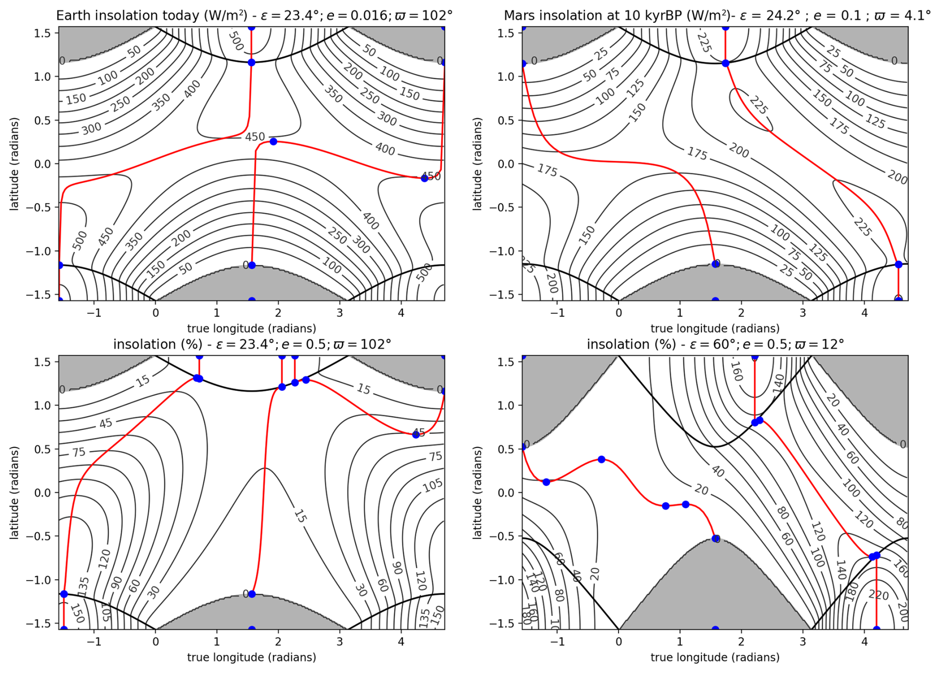
Figure 4Distribution of daily insolation as a function of “season” and latitude (both in radians). The “season” is measured through the true longitude of the Earth, with 0 being the NH-spring equinox. Polar night and day are delimited at high latitudes by a black line. In red, φExt(λ) indicates the location of minima and maxima. The blue dots correspond to the boundary values of the red curve in the polar day and night domains and to the points λM where φExt(λM) is extremal: these points λM (“turning points”) give us the latitudes φM=φExt(λM) beyond which the number of extrema changes. The curve φExt(λ) usually consists of two separate branches: a “polar-day-to-polar-day” branch (H-branch) and a “polar-night-to-polar-night” one (L-branch). Top-left: for present-day values of the orbital parameters. We note that the L-branch of φExt(λ) has two “turning points” λM at low latitudes (blue points), therefore a double maximum insolation near the equator between the corresponding two latitudes φM=φExt(λM). Top-right: when using martian orbital parameters at 10 kyr BP, this low-latitude double maxima disappear for slightly higher eccentricity. For even higher eccentricity (bottom left) and/or obliquity (bottom right) the situation can be more complex, since the L-branch can reach the polar day region and splits into two parts (bottom left) or the curve φExt(λ) may have more minima and maxima (λM,φM) than today (blue points, bottom right). Note that the bottom panels correspond to fictitious planets: insolation is then expressed in percentage of the “solar” or “stellar” constant.
In the scientific literature, I have not found any systematic mathematical study of the minima and maxima of the daily insolation WD for a generic planet, at a given latitude and for arbitrary astronomical parameters (e, ε, ϖ). Still, extremal values are likely to be useful when discussing climatic implications. A rather straightforward procedure could be to compute numerically the minimum or maximum of WD as a function of λ to get directly the extremum. This may be valid in some specific context, when the number of extrema is known (or assumed known) in advance, but it is likely to fail when we do not know a priori how many maxima and minima there is. This is in particular true at low latitudes where we can shift from one annual maximum (the typical situation at mid-latitudes) to two maxima (the typical situation at the equator). The transition between these two cases depends strongly on the astronomical parameters in a non-trivial way. We can even identify earthly situations (low obliquity, high eccentricity) where the second maximum at the equator disappears. In the generic setting, there are many different possibilities with up to three or more maxima.
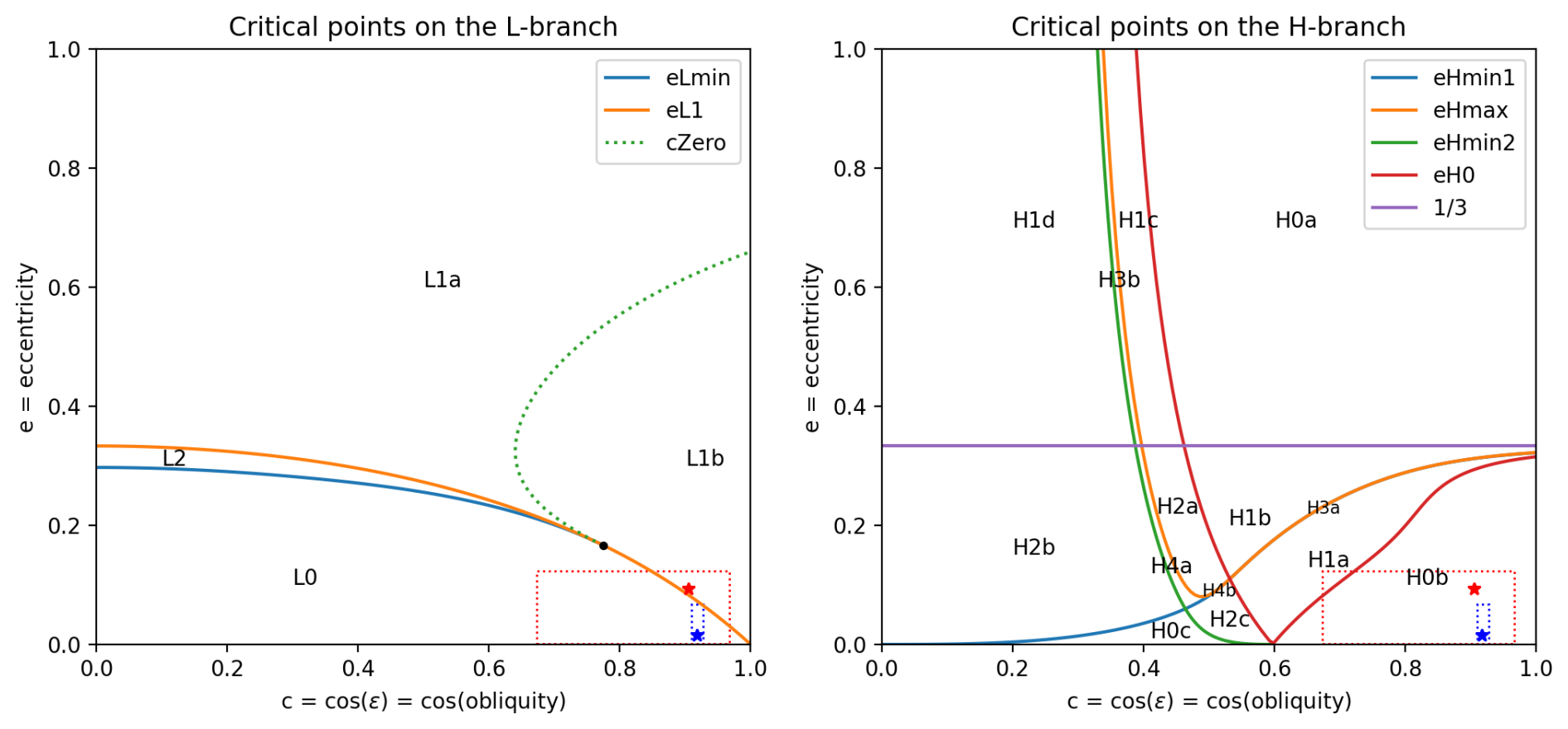
Figure 5Classification of the different possibilities for the L-branch (on the left) and for the H-branch (on the right) as a function of eccentricity and cosine of obliquity. Earth's present-day situation is the blue star and its past 100 Myr range is shown as a blue dashed box. Mars' present-day situation is the red star and its past 20 Myr range is represented by the red dashed box. For the L-branch, we can have 0, 1 or 2 critical values (ϖC,λC) in the intervals , corresponding to the different domains named L0, L1 and L2 shown on the figure, separated by colored curves. The L1 domain can itself be separated in 2 sub-domains (L1a, L1b) : in L1a we can have 2 or 4(λM,φM) solutions, while in L1b we can have 2 or 0 such solutions. In L0 there is always 2 solutions for (λM,φM) and in L2 we can also have 2 or 0 such solutions. For the H-branch, the situation is more complex with 14 different cases: we can have 0,1,2,3 or even 4 critical values (ϖC,λC) in the intervals , therefore the names of the domains H0 to H4. Domains H3a and H4b are extremely small, since the blue and orange lines (labelled eHmin1 and eHmax) are almost overlapping (see close-up in Appendix B). In the H0b domain, there is always 2 solutions for (λM,φM) which implies that there is some “hidden” extrema very close to the “polar-day” limit.
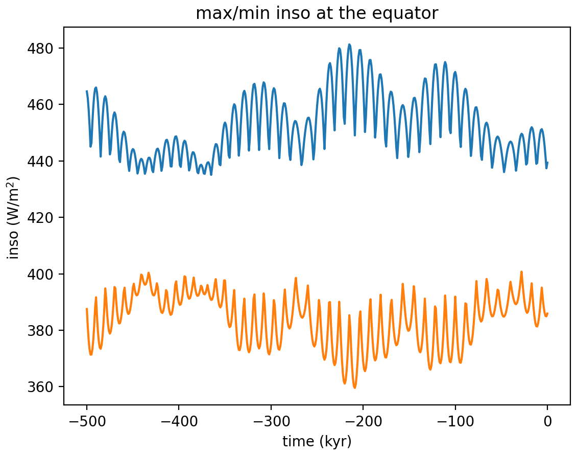
Figure 6Minimum and maximum daily insolation at the equator during the last 500 kyr. There is a clear semi-precessional signal since the maximum switches between times near the march equinox and times near the September equinox and, similarly, the minimum switches between solstices.
To obtain these extrema, the first step is to compute the mathematical derivation of WD with respect to λ.
The extrema are therefore given by:
where the function is strictly increasing for h between 0 (polar night) and π (polar day) and varies between 0 and infinity. It is therefore possible to define its inverse for any x≥0. Which leads to:
But h is defined as . We can therefore directly obtain the location of extrema using the equation:
plotted as red curves on Fig. 4 below.
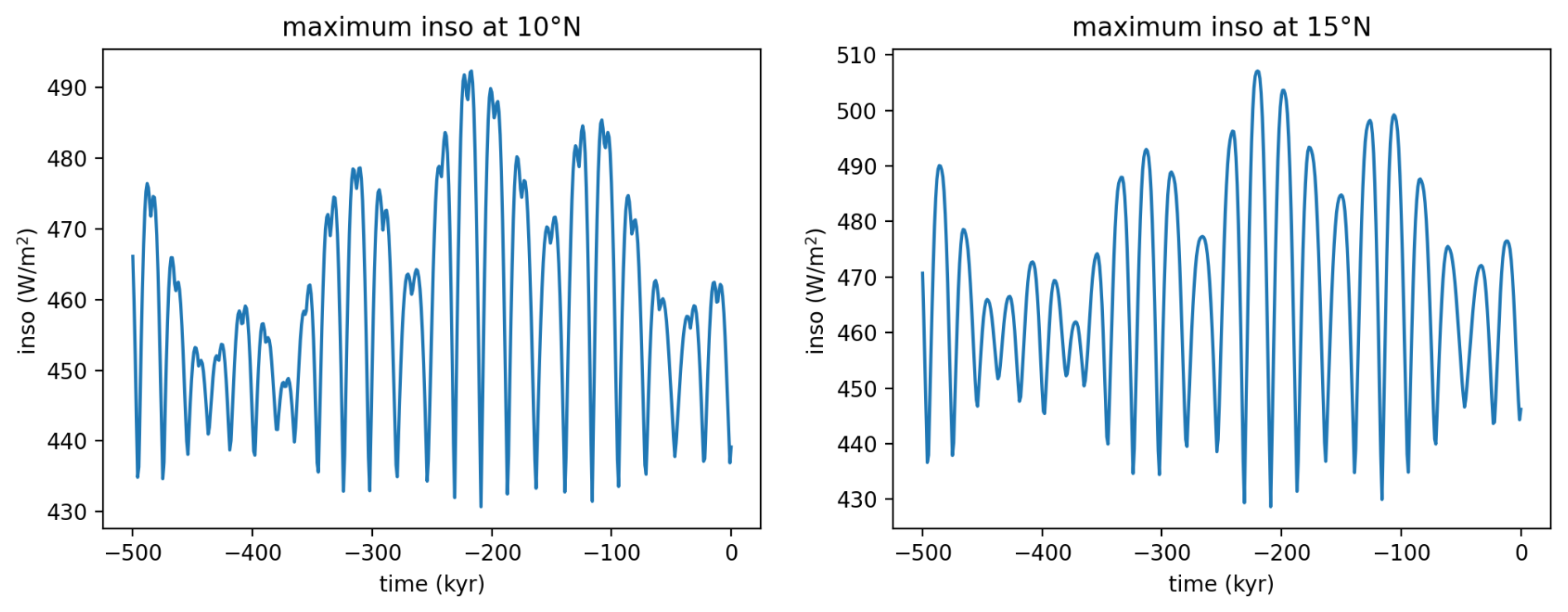
Figure 7The semi-precessional signal remains visible up to latitudes of about 10° but disappears for higher latitudes as shown above when looking at the maximum daily insolation at 10 and 15° N.
This is valid only when we have sunrise and sunset (for . Of course, during the polar night (h=0), we are constantly at a minimum (WD=0). The curve φExt(λ,…) will therefore intersect the polar-night domain precisely at and at (the solstices) with φExt being then the latitude of polar circles. During the polar day (h=π), the maximum (or possibly the extrema, see below) occur when:
This condition does not depend on latitude (nor on obliquity) and we can rather easily solve it to obtain the true longitude λPolarDay of the extrema for the polar day: this leads to a 4th degree polynomial equation (see Appendix B1) with usually 2 real solutions corresponding to the polar-day maxima in both hemispheres. But for , we can also obtain 4 solutions as shown on Fig. 4 (bottom left).
Unfortunately, Eq. (7a) gives us the latitude φExt of minima and maxima of the daily insolation WD as a function of orbital position, or true longitude, λ. But our goal was to do the opposite: for a given latitude, finding the longitude, or time of the year, when the daily insolation WD is extremal. For a given latitude φ, we thus need to solve in λ the Eq. (7a) in order to obtain the longitudes λExt. The key difficulty is, again, to know how many solutions this equation may have, as illustrated on Fig. 4.
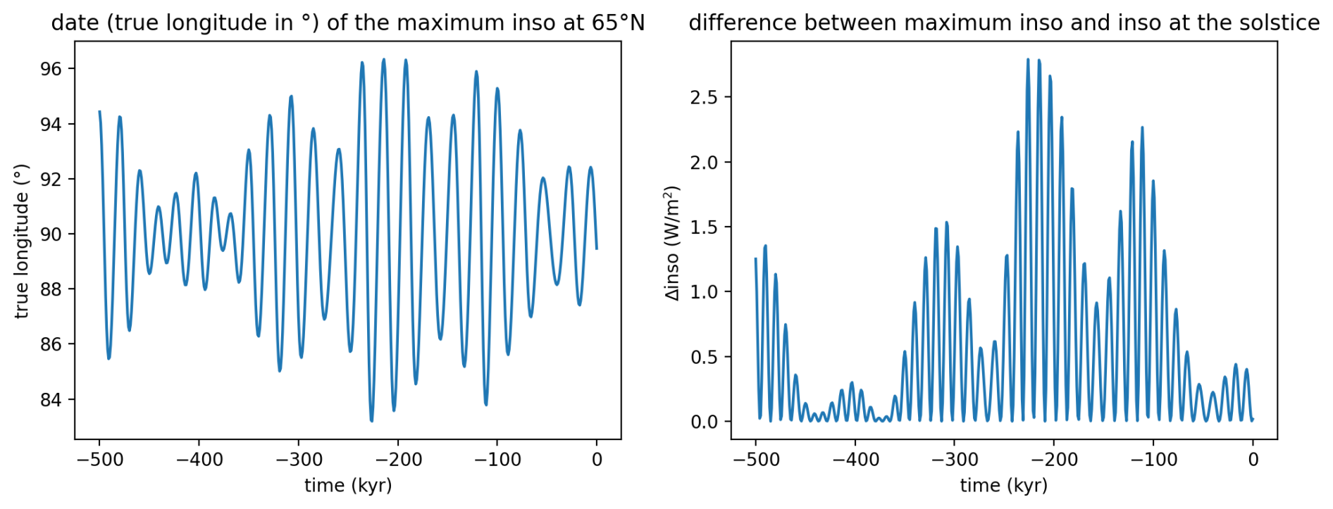
Figure 8The maximum insolation at 65° N over the last 500 kyr occurs for true longitudes λExt close to, but not equal to the summer solstice ( or 90∘) as shown on the left. The corresponding insolation difference (right panel) is quite small, but not entirely negligible.
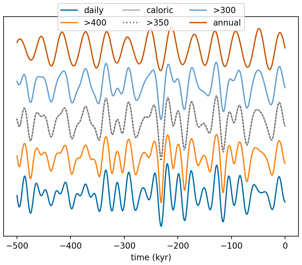
Figure 9Normalized summer insolations at 65° N defined in various ways. In blue (bottom) the daily summer solstice insolation. In orange, the integrated insolation above 400 W m−2. In green, the caloric summer insolation. In dotted red, the integrated insolation above 350 W m−2. In purple, the integrated insolation above 300 W m−2. In brown, the annual averaged insolation. The integrated insolation above 350 W m−2 is almost identical to the caloric summer insolation (green and dotted-red lines).
For Earth-like astronomical parameters, we can note that φExt as function of λ has two well-separated branches: a first one extending from polar night to polar night, that provides possible multiple extrema at low latitudes (latitudes between the blue dots on this branch) – it is referred to as the L-branch in the following – and a second branch from polar day to polar day – the H-branch –, that appears to generate only one maximum at any given latitude, something which will in fact be proven wrong in the following. Figure 4 also shows that the situation might become much more complex for other astronomical parameters (large eccentricity and/or large obliquity). In order to understand under which criteria these different possibilities may arise, and in order to find all possible extrema, we have performed a systematic study as summarized below.
We note that: . We also have: . We can thus limit our study to some interval like, for instance, and for the L-branch and and for the H-branch.
To get all roots λExt of Eq. (7a), we need to perform the mathematical derivation of with respect to λ and thus identify that satisfy both Eq. (7a) but also , represented by blue dots on the above figures. These points (λM, φM) are called “turning points” in the following. After some computation (see Appendix B2), this leads us to the equation in λ:
with as before.
But solving Eq. (8) might also gives multiple solutions for λM and we need to go another step further and locate the “critical” values λC that correspond to double-roots of Eq. (8). This is done (again) by taking the derivative of Eq. (8) and looking for the values of ϖ for which both Eq. (8) and its derivative can simultaneously be true. Knowing the number of such “critical” values for (ϖC,λC), we can obtain all possible values of λM and therefore all the extrema λExt, for any given situation. This allows us to classify all possible cases, depending on the number of such critical points. These critical points might be located on the 2 solutions branches already identified (details are given in Appendices B2 and B3), either at rather low latitudes (the L-branch) or at latitudes close to the “polar day” region (H-branch). The final results are shown on Fig. 5.
This systematic study is of course not always relevant for the Earth, with a rather low eccentricity (e usually smaller than 0.06) and moderate obliquity (c=cos ε usually larger than 0.9) as show by the dashed-blue box on Fig. 5. We will therefore not provide here a full inspection of all possible cases, though such a detailed discussion would easily follow from our study and the above figures. Concerning the H-branch, a surprise is that there is almost always a “turning point” (λM, φM), with φM located very near the latitude of the polar day and λM very close to the polar day value λPolarDay, even in the present-day situation (domain H0b on Fig. 5). Though it is not visible on the top panels of Fig. 4, we can see on the bottom panels (blue dots) that there is a (λM, φM) just near the polar day values (λPolarDay, φPolarDay). The difference is so small for the Earth's case (much smaller than 1° or 1 d between λM and λPolarDay) that is can certainly be neglected for all practical purpose.
A more relevant application of this study is to investigate the number of minima or maxima at low latitudes. Traditional thinking assumes that such minima or maxima occur near equinoxes and that it is sufficient to look at this two specific periods to discuss the corresponding semi-precessional forcing (Berger et al., 1997). But here again, it was a surprise to find that, concerning the Earth, the double annual insolation maxima can entirely disappear in some cases, even at the equator, when transitioning from domain L0 to L1b (for instance, eccentricity larger than 0.066 and obliquity smaller than 22°): in such situations, when perihelion is close to one equinox (ϖ is close to 0 or 180°) there is only one maximum and one minimum daily insolation whatever the latitude, since the role of the distance to the sun (the combined effect of e and ϖ on daily insolation) becomes larger than the role of obliquity. This situation actually happens frequently for planet Mars as shown on Fig. 4.
Since this systematic study allows us to find, for instance, all maxima at any given latitude and time, we obtain the maximum (the largest maxima) without difficulty. This is particularly useful to illustrate the semi-precessional forcing near the equator, as illustrated on Figs. 6 and 7.
Concerning higher latitudes, it is also worth examining whether the difference between insolation at the maximum and insolation at the summer solstice is significant or not. Indeed, the solstice is almost never strictly coincident with the maximum insolation, except when the perihelion occurs precisely at the solstice ( and it could be argued that, for instance, the maximum insolation at 65° N is climatically more relevant for the ice age problem than the summer solstice one.
It turns out that, concerning the Earth, the difference remains rather small (smaller than 2 or 3 W m−2) compared to about 500 W m−2: the relative difference is smaller than 0.5 % and the difference is strongly modulated by the eccentricity, as shown on Fig. 8. In any case, the python libraries provided here can be used to investigate and discuss these differences.
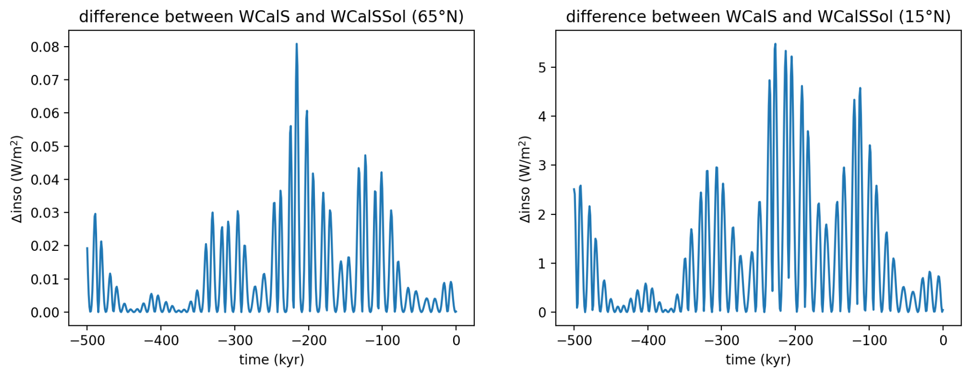
Figure 10Comparison of WCalS and WCalSSol at high northern latitudes (65° N) and at lower latitudes (15° N). The difference is negligible at 65° N (about 0.01 %) but becomes significant at lower latitudes. The approximation WCalSSol in the context of Quaternary glaciations is therefore very good and much faster to compute, while it might fail in other contexts, like lower latitudes or other planetary settings.
It was suggested that integrating the daily insolation above some threshold could be used as a relevant forcing when studying glaciations, since melting or freezing are themselves threshold processes (Huybers, 2006). The simplest way to produce the corresponding time series for Quaternary climates is to compute the daily insolation for every day of the year, then select and sum the ones above the chosen threshold. This might not be the most efficient way. Besides, discretizing the year into an integer number of days (360 or 365 d) as in Huybers (2006) (using the sum 86 400) is not entirely satisfying. Indeed, the number of days is not an exact integer and furthermore, such a discrete sum will change discontinuously when the threshold is modified continuously. Discretization itself might lead to slight numerical errors.
Overall, it is more direct, more precise and certainly more robust to compute all the true longitudes λT for which the insolation equals the threshold value (if any), and then integrate WD(λ) between them using Eq. (4). Indeed, from the above paragraph, we know how to compute the true longitudes λExt of minima and maxima of the daily insolation at any latitude and for any orbital configuration, as well as the associated extremal values of daily insolation WD(λExt). It is therefore quite straightforward to obtain numerically all the roots of the equation WD(λT)=WThreshold, identify the value(s) λT1 when WD increases above the threshold and the value(s) λT2 when WD decreases below WThreshold and finally integrate between the two as explained in Sect. 3. This is the strategy used in the routine “integrated_inso_above()” provided in the python library.
As illustrated on Fig. 9, the insolation integrated above some threshold is very similar to the daily summer solstice insolation when the threshold is chosen high enough and gets progressively closer to the annual average when the threshold is decreased. This is quite expected since the integral will cover a larger part of the year when the threshold is lowered. The role of the precessional component is then decreased accordingly up to a complete disappearance for the annual average. Interestingly, for threshold values near 350 W m−2, the result is almost identical to WCalS ≈WCalSSol, ie. the Milankovitch definition of insolation over the caloric summer.
But instead of using a fixed threshold, we can also use the same strategy in order to compute the Milankovitch insolation WCalS (the integral over a “caloric season”) for all possible orbital situations, even when the daily insolation has several maxima during the annual cycle, as this is the case in low latitudes today. As explained in Sect. 3.1, we first need to find the threshold value such that the insolation exceeds it during exactly half a year (the “caloric summer”). Since, for any threshold WThreshold, we can obtain as above the value(s) λT1 and the value(s) λT2 for which WD(λT) crosses it upwards and downwards, we can also compute the associated mean longitudes LλT1 and LλT2, and the corresponding duration(s) LλT2−LλT1, and finally sum up all these durations in case there are several such intervals. In other words, it is quite straightforward to define a function f(WThreshold) that computes the time during which the insolation remains above the threshold. By solving , we get the desired value of WThreshold and the caloric summer mean insolation WCalS can then be computed as the integral above this threshold, using the above procedure.
When comparing WCalS (insolation over the caloric summer) to its approximation WCalSSol (insolation over the half year centered at the solstice) as shown on Fig. 10, we note that the difference is very small for the Earth at high northern latitudes. It is therefore fully acceptable to approximate WCalS with WCalSSol and the approximations used by Milankovitch were in fact quite similar to the ones used here in WCalSSol. Interestingly, the difference (about 0.01 %) is much smaller than the one between maximum insolation and insolation at the solstice, as shown on Fig. 8 (about 0.3 %), an approximation that many people are using without further caution.
There are probably countless possible “flavours” of different insolation quantities. Overall, testing the response of simple ice age models to such different possible choices is certainly quite crucial (Leloup and Paillard, 2022). The objective was here to present and rapidly discuss the ones that have been mentioned in the paleoclimate scientific community. Some of the formulas presented in this paper are very classical, while others are new, especially the ones concerning the computation of minima and maxima. The python library is described in more details below in Appendix A. It is designed to experiment easily with these various kinds of “insolations”. Most of these routines were initially written in C and embedded in the “AnalySeries” MacOS software (Paillard et al., 1996). The version presented here is written in Python for an easier and wider access. It can be easily installed using the command “pip” (pip install inso). It is now used in the new version “PyAnalySeries” released recently (Hevia-Cruz et al., 2025).
All the formulas discussed in this paper are implemented in python and all the figures shown here can be reproduced with the python file “figures.py”: they can be used as examples for using the python routines. The library itself is organised in 3 different files: “astro.py”, “inso.py”, “minmax_inso.py”.
A1 Library “astro.py”
This library provides a useful uniform interface to different astronomical solutions that have been published. The first step is to choose the desired solution by defining the corresponding object: the reference solution is currently the Laskar et al. (2004b) and it is usually necessary to start with the line:
Currently, other possibilities are the objects: AstroBerger1978(); AstroLaskar1993_01(); AstroLaskar1993_11(); AstroLaskarMars2003(); AstroLaskarMars2004(); AstroLaskar2010a(); AstroLaskar2010b(); AstroLaskar2010c(); AstroLaskar2010d(); StockwellPilgrim1904(). Other astronomical solutions will be added in future releases.
Time t is expressed in kyrAP (thousands of years after present), which means that t is positive in the future and negative in the past. The user should be aware that the starting time is different for these different solutions: for Laskar's solutions, t is in thousands of years after 2000 AD; for Berger's solution, t is in thousands of years after 1950 AD; for Stockwell's solution, t is in thousands of years after 1850 AD.
This information, as well as the original references, can be easily obtained by calling the “info()” function which is returning a string:
For each solution, it is possible to check whether orbital parameters are available for some desired time t using the boolean function:
The “Laskar2004” solution is available in the range 101 MyrBP to 21 MyrAP.
The “Berger1978” or the “StockwellPilgrim1904” solutions are given for historical purpose: they are trigonometric approximations: Berger (1978a) is based on Bretagnon (1974) and Pilgrim (1904) is based on Stockwell (1873). As such, there is no implemented time limit (the function in_range() returns always True), but the validity is probably restricted to about 1 million years in the past or the future for “Berger78” and much less for “StockwellPilgrim1904”.
The “LaskarMars” solutions (available in the range 21 MyrBP to 11 MyrAP) apply to planet Mars, while all the other ones concern planet Earth.
The “Laskar1993_01” and “Laskar1993_11” (available in the range 20 Myr BP to 10 Myr AP) differ in the way the dynamical ellipticity of the Earth is treated, something that affects the computation of precession and obliquity on the million-year time scale. Comparing these two solutions gives some idea of the associated uncertainties.
The “Laskar2010x” solutions (available in the range 249.999 Myr BP to today) only provide the eccentricity and therefore cannot be used to compute the insolations discussed in this paper. It is nevertheless interesting to compare them in order to better understand the range of validity of the eccentricity and to look how they start to diverge beyond about 50 Myr.
For all these solutions (except “Laskar2010x”) we have access to the climatically relevant astronomical parameters (eccentricity e, obliquity ε, climatic precession angle ϖ) at time t through the function:
-
a.eccentricity (t)
-
a.obliquity (t)
-
a.precession_angle (t)
It is also useful to define a “climatic precession parameter” as esin ϖ which is directly given by the function:
-
a.precession_parameter(t)
Angles (obliquity ε and climatic precession angle ϖ) are expressed in radians.
A2 Library “inso.py”
From the astronomical parameters obtained through the above routines, it is then possible to compute the insolation quantities described in the paper. In order to be as generic as possible, the results are always returned in a dimensionless form: the same routines can therefore be applied to any planet. But it is necessary to multiply the result by the corresponding dimensional quantity (for instance the solar constant, the duration of the day or of the year in the preferred units).
To obtain the instantaneous insolation from Eq. (1), for example concerning Earth, at noon, at 45° N, at the summer solstice, 10 kyr BP, we can write:
-
solarCte=1365 # the solar constant in W m−2
-
H=0 # the hour angle: noon = 0
-
# the latitude in radians
-
# the true longitude of the Earth at the summer solstice, in radians
-
# 10 thousand year before present
-
ecc = a.eccentricity (t)
-
obl = a. obliquity (t)
-
pre = a.precession_angle (t)
-
WI = solarCte ∗ inso_radians (h, trueLon, lat, obl, ecc, pre)
In the same way, we can get the daily insolation from Eq. (2):
-
WD = solarCte ∗ inso_ dayly_radians (trueLon, lat, obl, ecc, pre)
As mentioned in the main text, this quantity depends mainly on two terms: the length of the day between sunrise and sunset (in dimensionless form ) and the height of the sun (measured by the averaged cosine of the zenith angle 〈cos z〉. These two terms can be obtained through:
-
# in hours
-
meanCosZ = inso_mean_cosz (trueLon, lat, obl)
It can be useful to measure the position of the Earth on its orbit using time (or, in dimensionless form, mean longitude or mean anomaly) instead of true longitude or true anomaly. To perform these conversions, we have the following routines. To solve the Kepler Eq. (3) and compute the eccentric anomaly E, or the true anomaly v, from the mean anomaly M:
-
E = solveKepler (ecc, M)
-
v = trueAnomalie (ecc, M)
And the converse:
-
M = meanAnomalie (ecc, v)
Or to get the true longitude from the mean longitude:
-
trueLon = trueLongitude (meanLon, ecc, pre, refL = 0)
where refL is the reference true longitude, by default equal to the NH-spring equinox (=0).
It is also possible to obtain the time needed to go for one orbital position (true longitude = trueLon1) to the next (trueLon2) using the routine:
-
delta_t = 365.25 ∗ length_of_season (trueLon1, trueLon2, ecc, pre) # in days
like, for instance, the duration of NH-summer (from NH-summer solstice to HN-automn equinox):
-
summer_duration = 365.25 ∗ length_of_season (90∗ np.pi/180, 180∗np.pi/180, ecc, pre) # in days
Using these conversions from mean longitude (time) to true longitude, it is possible to compute the daily insolation at some calendar date, which means a given number of days (or mean longitude) measured from a reference true longitude (refL):
-
WD = solarCte ∗ inso_ dayly_radians (trueLongitude(meanLon, ecc, pre), lat, obl, ecc, pre)
Or, as a shortcut:
-
WD = solarCte ∗ inso_dayly_time_radians (meanLon, lat, obl, ecc, pre)
(beware that this is NOT what people usually want to do when discussing paleoclimate... see main text).
If we prefer to use the averaged insolation over some part of the annual cycle, between two orbital positions trueLon1 and trueLon2, as in Eq. (4), we can use the routine:
-
W12 = solarCte ∗ inso_ mean_radians (trueLon1, trueLon2, lat, obl, ecc, pre)
The result has the same units as the solar constant (usually in W m−2). Of course, if instead we want the integral (in J m−2), we need to multiply by the duration of this interval :
-
J12 = solarCte ∗ inso_ mean_radians (trueLon1, trueLon2, lat, obl, ecc, pre) ∗ 365.25 ∗ 24 ∗ 3600 ∗ length_of_season (trueLon1, trueLon2, ecc, pre)
And if we prefer to refer to orbital positions in terms of mean longitude, we can use:
-
WD = solarCte ∗ inso_ mean_time_radians (meanLon1, meanLon2, lat, obl, ecc, pre)
A specific example of this last routine are the approximation of insolation over caloric seasons (as integrals over the half-year centered on the solstices). For the caloric northern hemisphere summer, we have:
-
WcalSSol = solarCte ∗ inso_mean_ time_radians (−np.pi/2, np.pi/2, lat, obl, ecc, pre, np.pi/2)
Or, as a shortcut:
-
WcalSSol = solarCte ∗ inso_caloric_summer_NH (lat, obl, ecc, pre)
And similarly for the caloric northern hemisphere winter:
-
WcalSSol = solarCte ∗ inso_caloric_winter_NH (lat, obl, ecc, pre)
These approximations are very good in the context of Quaternary glaciations. A more generic and precise algorithm to compute WcalS (WcalW) is provided in the library “minmax_inso.py” described below.
As mentioned in the main text, the daily insolation can also easily be integrated between different latitudes, lat_a and lat_b, as in Eq. (5). This is done with the routine:
-
Wab = solarCte ∗ inso_mean_lat_radians (trueLon, lat_a, lat_b, obl, ecc, pre)
And finally, as in Eq. (6), we can integrate both of part of the seasonal cycle between trueLon1 and trueLon2, and also between latitudes lat_a and lat_b. This is implemented as:
-
W12ab = solarCte ∗ inso_mean_lon_lat_radians (trueLon1, trueLon2, lat_a, lat_b, obl, ecc, pre)
If we prefer to integrate insolation only over some part of the day, between sun hour-angles h1 and h2, we can use:
-
JH = 86400 ∗ solarCte ∗ inso_radians_integ (h1, h2, trueLon, lat, obl, ecc, pre) # in J m−2
And the over latitudes lat_a and lat_b:
-
JHab = 86400 ∗ solarCte ∗ inso_radians_integ2 (h1, h2, trueLon, lat_a, lat_b, obl, ecc, pre) # in J m−2
A3 Library “minmax_inso.py”
While many of the routines available in “astro.py” and “inso.py”, as described above, are available in several other software packages or languages, the routines in “minmax_inso.py” are, to my knowledge, entirely new. As described in the main text and in the following annex, the mathematical derivation is rather tricky and cumbersome. There are consequently numerous routines in the code that might not be directly useful to users.
Probably one of the most simple uses of this library is the computation of the largest daily insolation maximum at some given location. For instance, at 5° S this can be obtained through:
-
solarCte = 1365 # the solar constant in W m−2
-
lat 5 ∗ np.pi/180 # the latitude (5° S) in radians
-
Wmax = solarCte ∗ largest_max (lat, ecc, obl, pre)
We can also retrieve the smallest minimum by:
-
Wmin = solarCte ∗ smallest_ min (lat, ecc, obl, pre)
The full list of daily insolation minima and maxima can be obtained through:
-
list = minmax_dayly_inso (lat, ecc, obl, pre)
It is a 2D numpy array with list[i][0] being the true longitude of the extrema (in radians) and list[i][1] being the corresponding value of the routine inso.inso_dayly_radians( list[i][0], lat, obl, ecc, pre).
This array is the concatenation of the two lists corresponding to the L-branch and H-branch, obtained through:
-
L_minmax(lat, ecc, obl, pre) and H_minmax(lat, ecc, obl, pre)
Another useful routine presented in the main text is the computation of integrals above some threshold. This is obtained through the routine:
-
solarCte = 1365 # the solar constant in W m−2
-
year = 365.25 ∗ 24 ∗ 3600 # the duration of the year in seconds
-
thresh = 350/solarCte # the threshold as a dimensionless value
-
JT = solarCte ∗ year ∗ integrated_inso_above (thresh, lat, ecc, obl, pre) # in J m−2
It is also possible to compute the insolation received during the “caloric seasons” (for example during the caloric summer) in the most generic settings, using the routine:
-
WCalS = solarCte ∗ inso_caloric_summer (lat, ecc, obl, pre) # in W m−2
Most of the other routines in this library are for internal use. They might nevertheless be interesting for people who would like to look in more details at this question of insolation extrema. To compute them, it is necessary to build a list of both the boundaries, either λPolarDay or , and of the “turning points” λM given by the solutions of Eq. (8): the extrema are then located between two successive values of this list. For respectively the L-branch and the H-branch, we obtain these lists by calling:
-
L_branch(ecc, obl, pre) and H_branch(ecc, obl, pre)
The λM values are themselves obtained respectively by:
-
lbd_minmaxL(ecc, obl, per, critPoints) and lambda_minmaxH(ecc, obl, per, critPoints)
where the variable “critPoints” contains information on the critical λC values and is obtained through the routines
-
lbd_critL(ecc, c) and lbd_critH(ecc, e)
where c= np.cos( obl ).
The library also contains the definition of the boundaries for the different domains illustrated on Fig. 5 as well as several plotting routines useful to examine the mathematical problem, notably:
-
plot_Ldomains() and plot_Hdomains()
used to draw Figs. 5 or B4, and plot_Hdomains_zoomed() to draw Fig. B9.
The summary plots shown on Fig. 4 are obtained with the routine
-
plot_inso_with_min_max (solarCte, ecc, obl, pre)
B1 Solving Eq. (7b)
The domain of definition of φExt (shown on Fig. B1) may start or end on the polar-day region at the true longitude λPolarDay corresponding to the Eq. (7b):
Note that λPolarDay depends only on e and ϖ. With , Eq. (7b) is equivalent to:
this last expression being preferred, since it is continuous everywhere with the standard definition of arctan(), with k being some integer. When the function ϖ(x) defined as above is monotonous, there is a unique inverse function ϖ−1() and therefore two solutions for x: and .
The derivative is zero when , which is possible only when , ie. when . In other words, ϖ(x) is always decreasing for and Eq. (7b) has then only two solutions or corresponding to summer in both hemispheres.
But when we might have two additional solutions for with:
More precisely, Eq. (7b) is equivalent to:
Using , (with , we have:
This is a 4th degree polynomial equation in t that can be solved by standard techniques. As explained above, there will be always at least two real roots t1 and t2 and when and we will also have two additional real roots t3 and t4. For each one, we can compute the corresponding true longitude of the “polar-day” extremum: . The two first roots are the true longitude of the bounds of the H-branch of φExt(λ) while the eventual two last ones are the intersection of the L-branch with the polar-day limit.
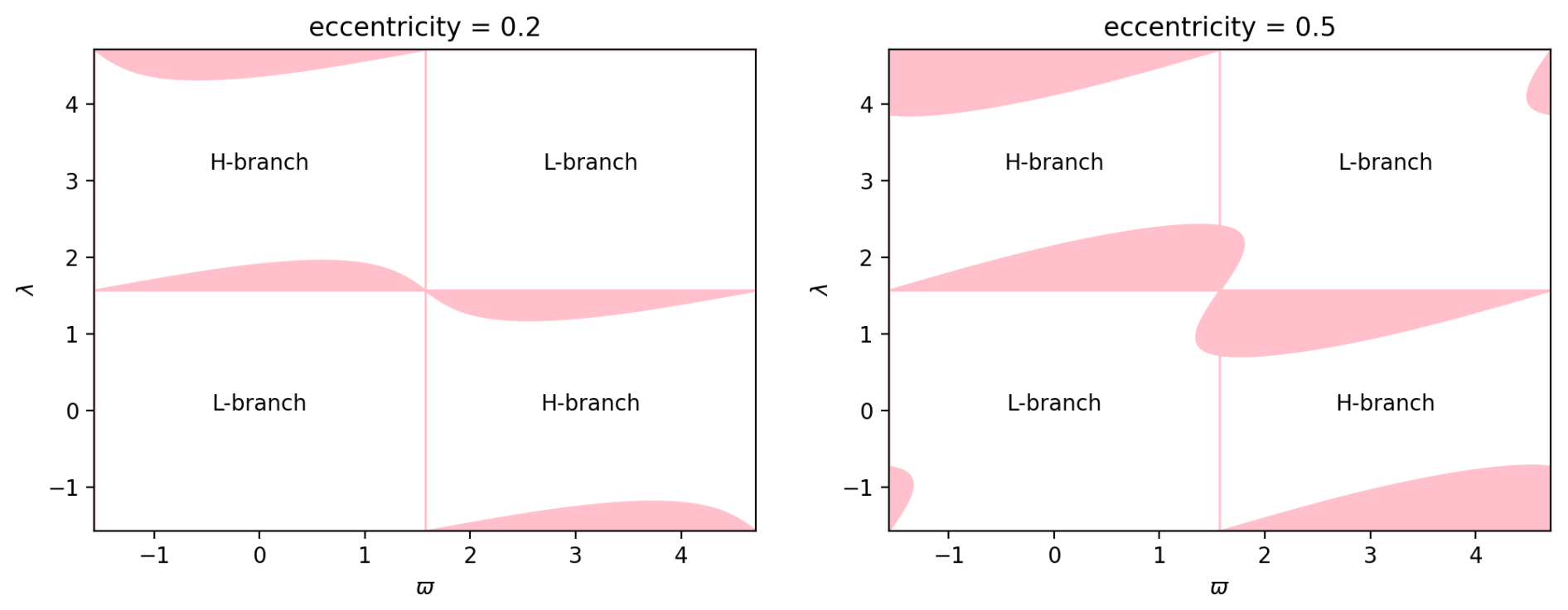
Figure B1The domains of definition of for the L-branch and H-branch, for two different values of the eccentricity: on the left e=0.2 and on the right e=0.5. For low eccentricity (, for a given value of ϖ, the L-branch starts and ends on the polar night with while the H-branch starts and ends on the polar day regions with λ=λPolarDay the two reals roots of Eq. (7b). For high eccentricity () the L-branch also intersects the polar-day region when ϖ is near at the two supplementary roots of Eq. (7b) as shown on Fig. 4b.
B2 Finding Eq. (8)
Equation (7a) gives us the latitude φExt of the extrema of the daily insolation WD as a function of true longitude λ; in other words, it defines . To obtain the minima and maxima of this curve, we want to compute its derivative and solve in order to find the corresponding true longitude λM.
First it is useful to introduce some new notation:
We can check that:
and then we can write Eq. (7a) in the following way:
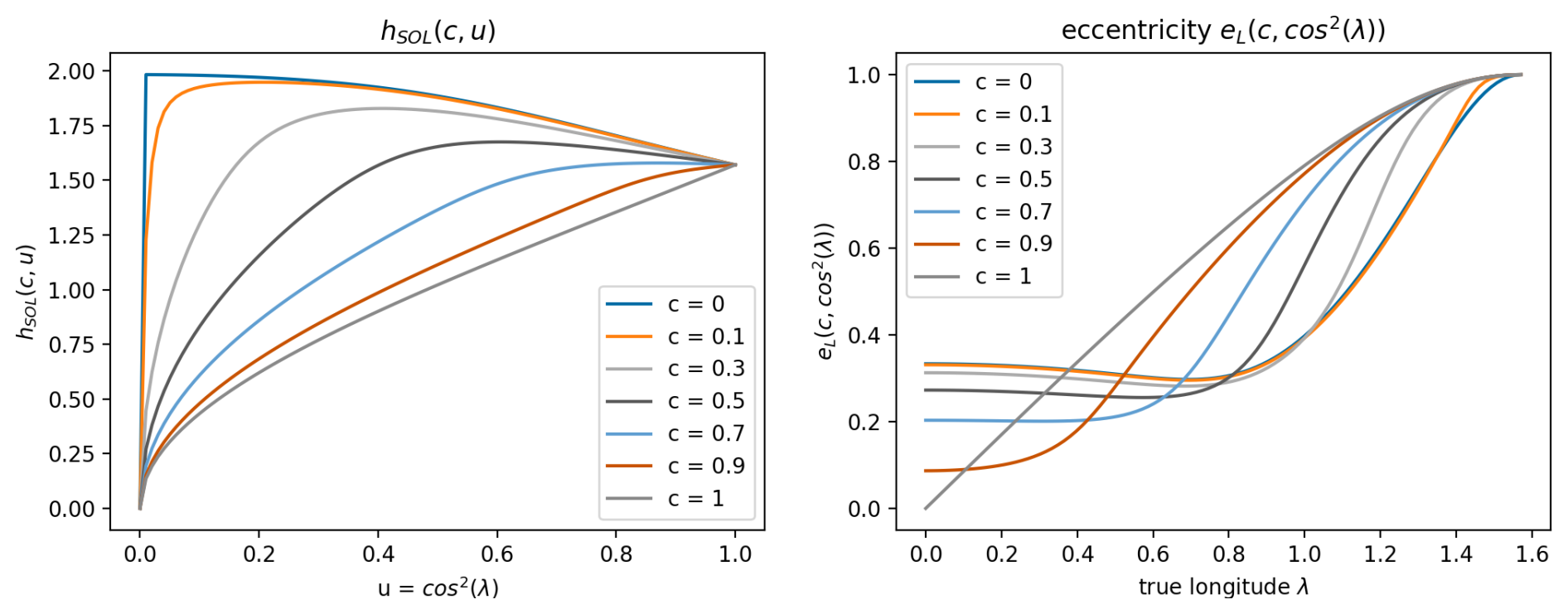
Figure B3Left: solutions of Eq. (B5) for various values of c. Right: the corresponding values of eL(c,cos 2λ) using Eq. (S6). Critical points λC (when they exist) are obtained by solving in λC the equation for some given (eε).
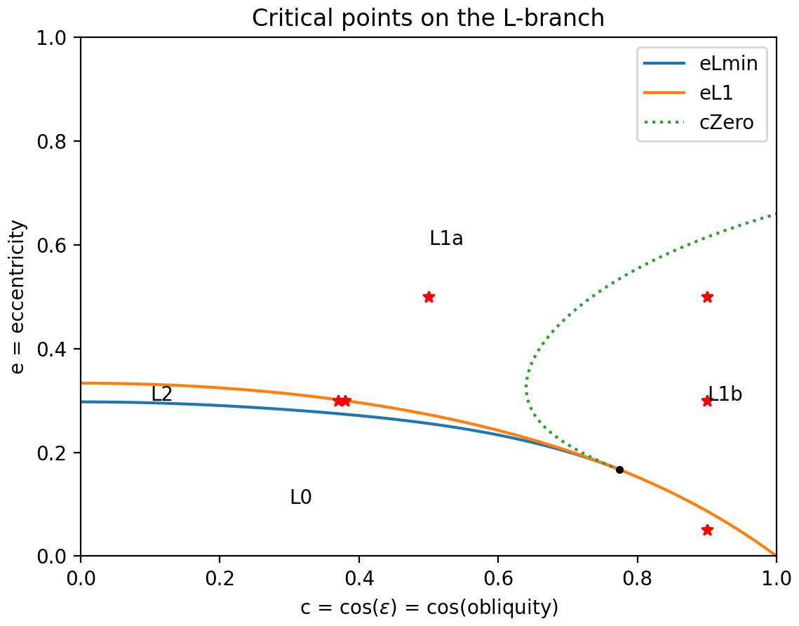
Figure B4In the ) space (top), the regions for which has 0, 1 or 2 solutions λC (L0, L1, L2) delimited by (orange) and by e=eLMIN(c) (blue), which cross at (black dot). The L1 domain is itself divided in 2 parts (L1a, L1b) depending on the relative positions of the critical solutions (cf. next figure). The red stars corresponds to the different situations illustrated in Fig. B5.
We look for λM such that or equivalently for w such that .
That is:
or equivalently:
But h is defined also by the 2nd equation of (B1):. We have therefore to compute its derivative and introduce the above new constraint in it, in order to obtain Eq. (8). We have:
To compute it is useful to introduce further new notations:
where we can check that:
This gives us:
Therefore:
By summing up Eqs. (B2a, b, c), we get:
In other words, as mentioned in the main text, Eq. (8) reads:
with
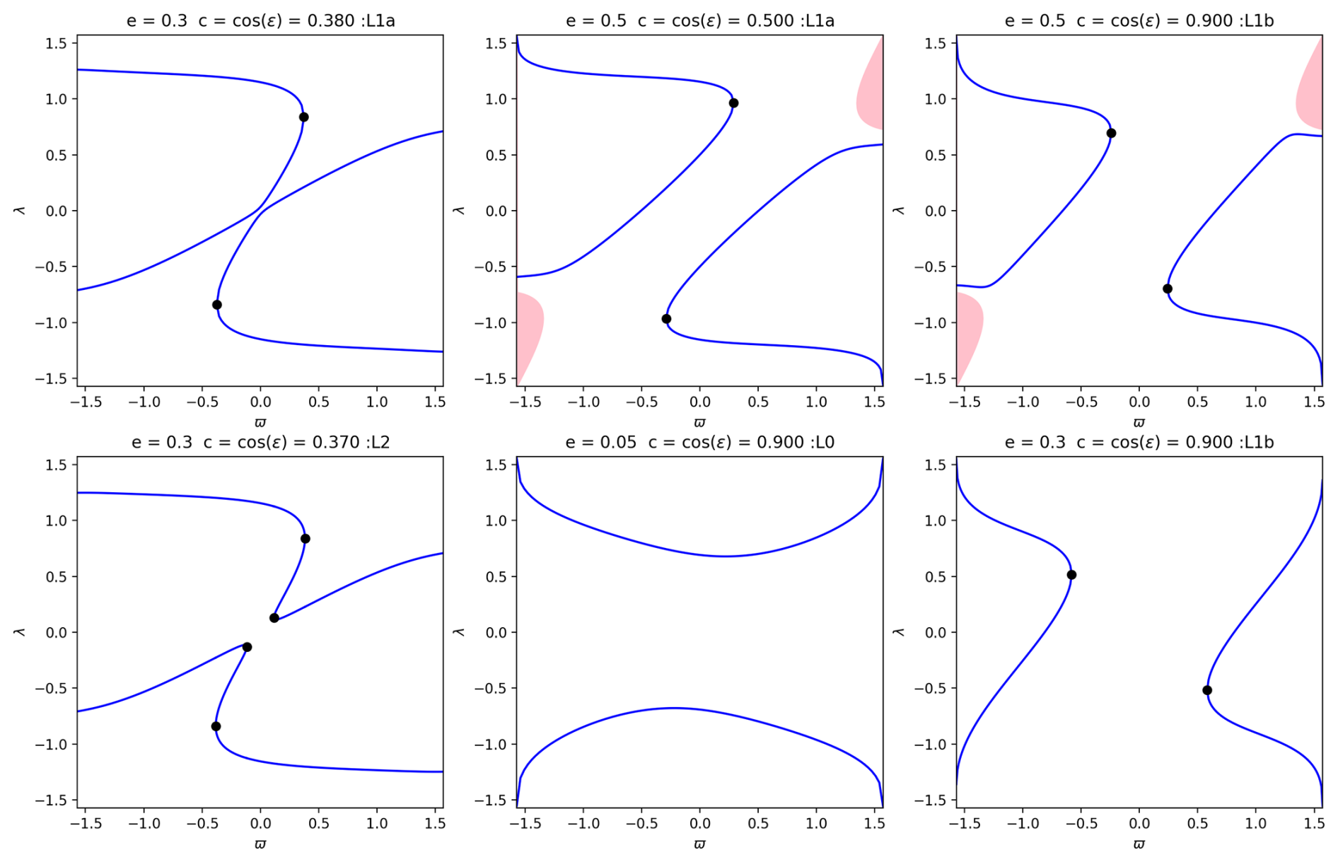
Figure B5Examples showing the values of λM (blue lines) as functions of ϖ, with branches delimited by the critical points (ϖCλC) (black dots) for the (c,e) parameters shown as red stars in the previous figure. In the L0 case (middle down panel), there are two extrema λM for every value of ϖ, corresponding the Earth's situation at low latitudes. In the L1b case (right panels), the critical points (ϖCλC) are in the top-left/bottom-right quadrant: there are either two extrema λM for a given value of ϖ, like before, or no such extrema when ϖ is near 0 (or π), more precisely for . In the L1a case (left and middle top panels), the critical points (ϖCλC) are in the top-right/bottom-left quadrant: there are either two or four extrema λM depending on ϖ. In the L2 case (left bottom panel), there are also either two or four extrema λM depending on ϖ with respect to the critical points.
B3 Classifying all possible cases for the minima and maxima
To obtain all values of true longitude λ for minima and maxima at a specific latitude φ, we can solve Eq. (7a) numerically with λ between successive values of λM since there is one and only one such root. But to find all possible values of λM, we also need to solve Eq. (8) numerically, with λM between successive values of λC which are roots of Eq. (8) and of its derivative.
To obtain these critical λC values, in addition to Eq. (B3) we therefore need to solve:
We have:
The definition of g gives us:
Therefore:
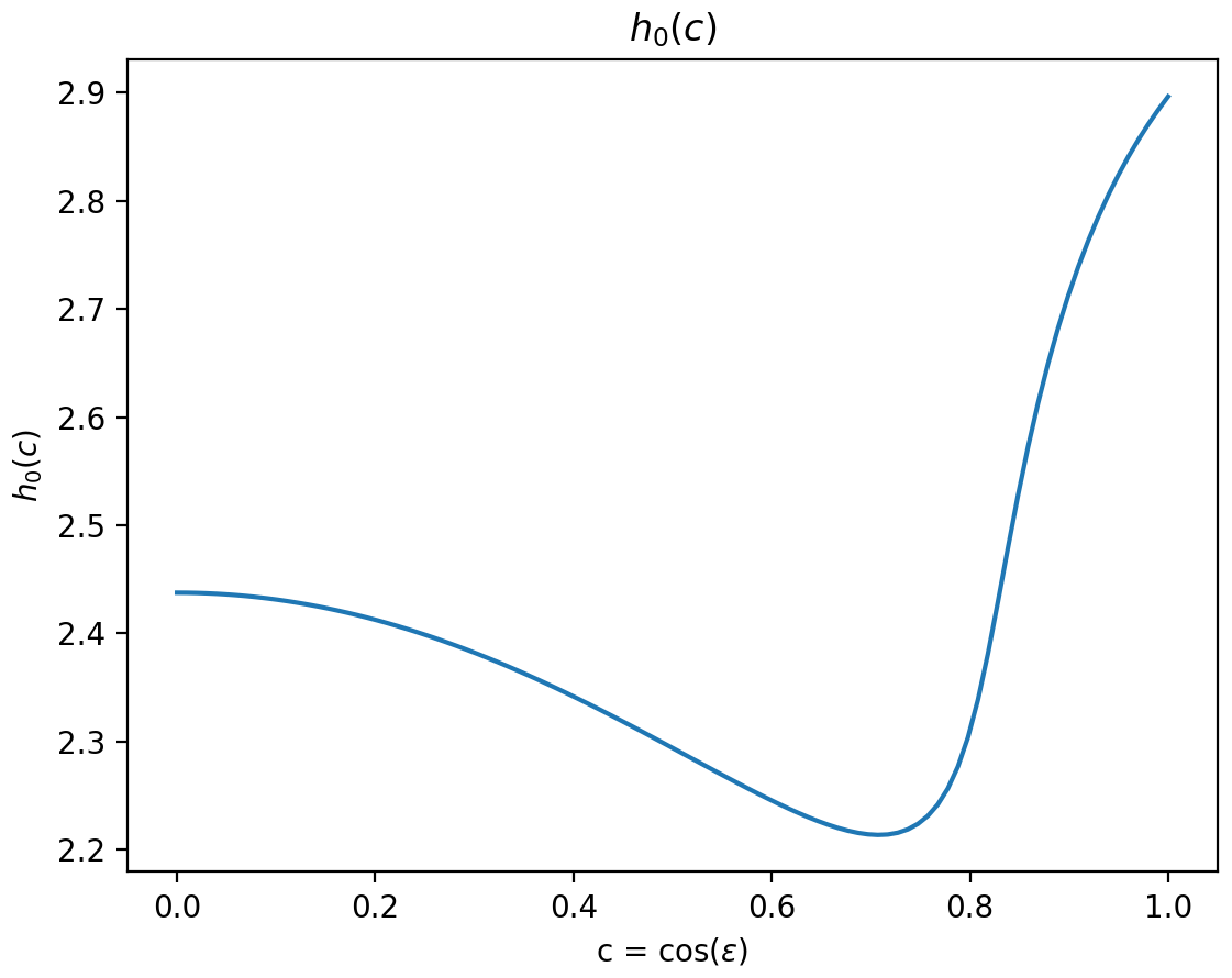
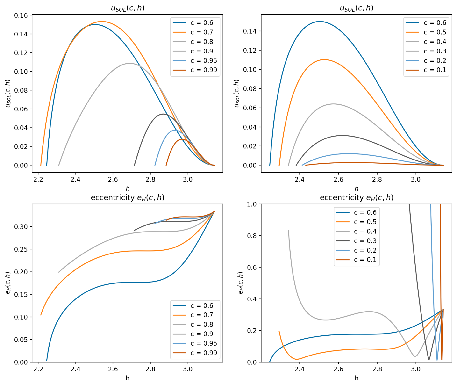
Figure B7Top: uSOL(c,h) for various values of c, in the increasing (left) and decreasing (right) ranges of h0(c). Bottom: the corresponding values of the eccentricity eH(c, h) using Eq. (B6). Critical points λC (when they exist) are obtained by solving in h the equation for given (e,c): the number of such points depends on the value of e with respect to the bounds and extrema of these curves.
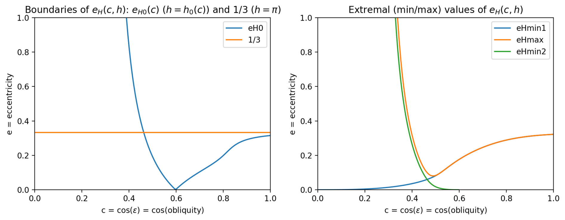
Figure B8Left: the end-points of eH(c,h) for h=π (in orange ) and for h=h0(c) (in blue ). The eH0(c) curve starts at the point {c0S,1}, has a cusp point at {c0R,0}, and ends at the point {1,eH0(1)}. Right : Extrema of the function eH(c,h): the minima eHMin1(c) in blue and eHMin2(c) in green, and the maximum eHMax(c) in orange. The minimum eHMin1(c) (blue) is defined for all values of c and eHMin1(0)=0 and eHMin1(1)≃0.322038. The minimum eHMin2(c) (green) is relevant (smaller than 1) for and defined for c<c0R the cusp point of eH0(c). The maximum eHMax(c) is relevant (smaller than 1) for .
Therefore, we have the equation:
But from Eq. (B3) we also have: . Therefore:
We finally get the equation satisfied by the critical points λC:
Using again some new notation:
We have:
And we can write Eq. (B4) as an equation only in ():
using:
For a given c=cos ε, as shown on Fig. B2, we note that this Eq. (B5) has two well separated branches: a first branch with h≤2, that can be described by a solution and a second one with h>2 (in fact, , see below) which is given by a solution .
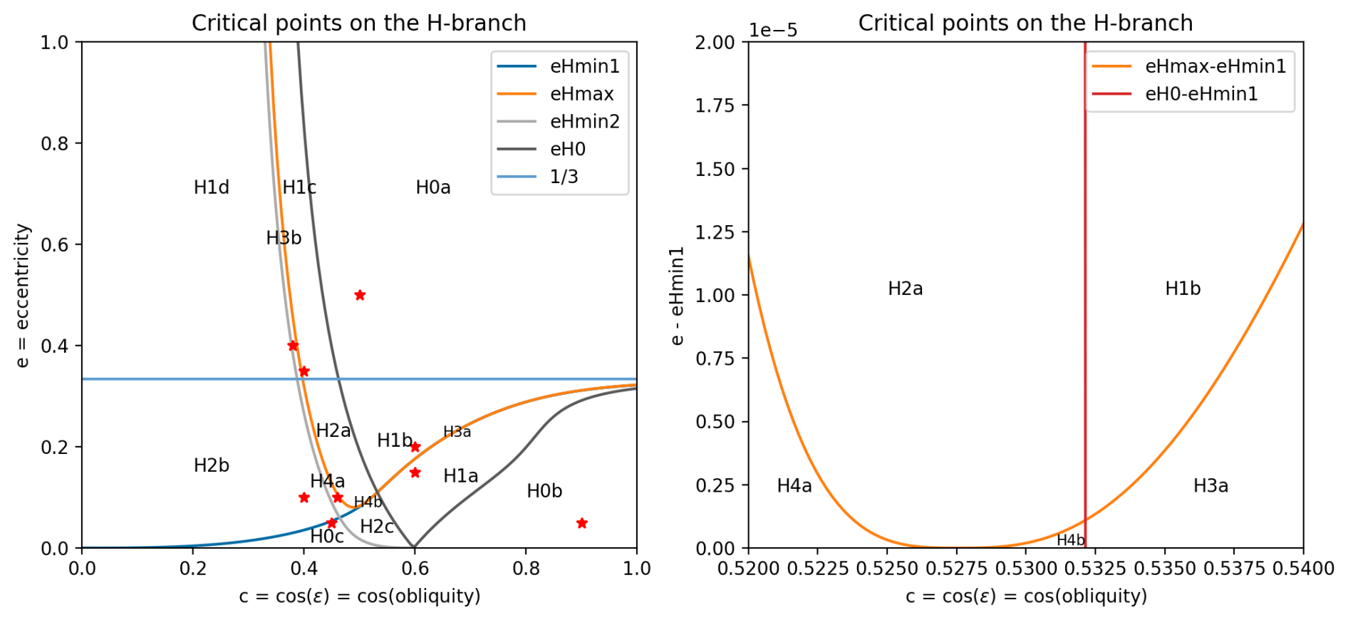
Figure B9On the left, in the space, the 14 regions for which has 0, 1, 2, 3 or 4 solutions λC. The red stars corresponds to the different situations illustrated in Fig. B10. On the right, a close up around the H4a domain: note that this is the difference e−eHMin1(c) and the vertical axis is strongly enlarged since eHMax(c) and eHMin1(c) are extremely close to each other (difference is about 10−4 or 10−5).
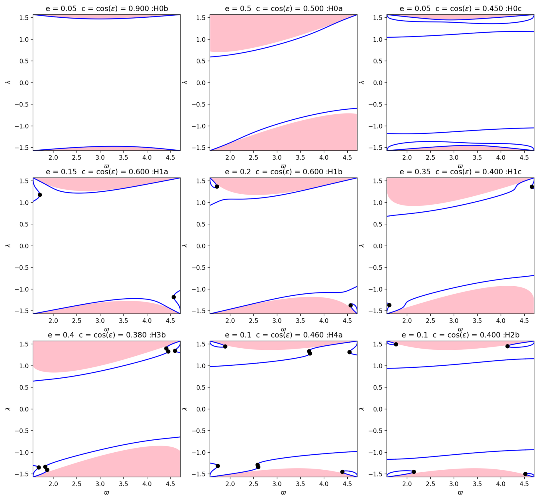
Figure B10Examples showing the values of λM (blue lines) as functions of ϖ, with branches delimited by the critical points (ϖCλC) (black dots) for the (c,e) parameters shown as red stars in the previous figure. In the H0b case (top left) ie. the Earth situation, there is always an extremal value λM very close to the polar-day limit (pink areas). Other various cases are also illustrated.
These two solution branches uSOL(c,h) and hSOL(c,u) do, in fact, correspond to the H-branch and L-branch mentioned in the main text. But uSOL(c,h) and hSOL(c,u) are still implicit since we are looking for the corresponding functions ϖC(c,e) or λC(c,e). This last step is easily obtained by noting that f, g and w are linked to the eccentricity e in the following way:
Substituting as above, we can write e as a function of our variables :
with:
Solutions of Eq. (B5) can therefore be written as:
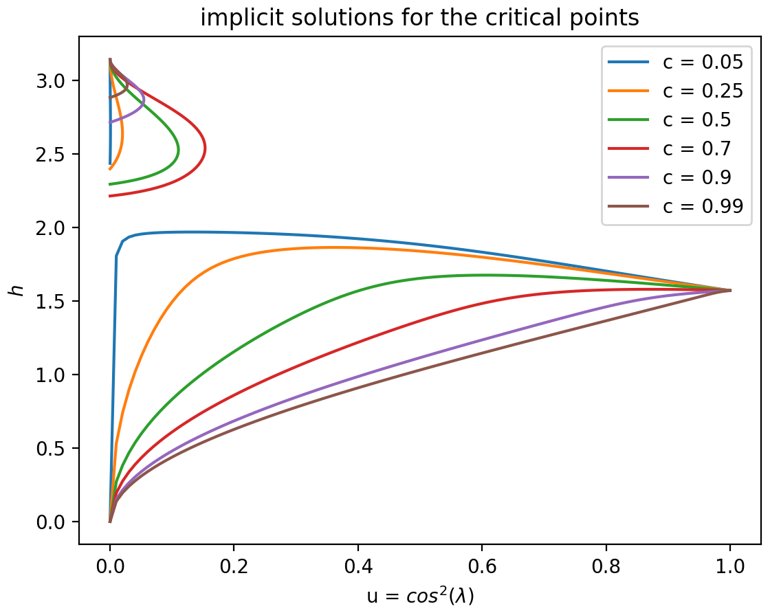
B3.1 L-branch solution h=hSOL (c,u) or e=eL (c,u)
We have and for all values of c. The derivative at u=1 can be obtained through Taylor expansion of Eq. (B5):
Critical values (λC, ωC) are obtained by solving e=eL (cosε, cos2λ) for given astronomical parameters (e,ε). Depending on c, we see on Fig. B3 (right panel) that there is 0, 1 or 2 solutions. The end points are:
We remark (cf. Fig. B3, right panel) that eL (c,u) has a minimum when c is small enough (when ε is large enough). This happens when the derivative d is negative for λ=0 i.e. (or ε>39,23°). Therefore, for we can compute (numerically) a minimum eLMIN(c).
To summarize, we end-up with three possibilities:
-
if , there is only one critical value (λC, ωC).
-
if and , we have two critical values (λC1, ωC1), (λC2, ωC2).
Otherwise, there is no critical value.
We have therefore the three domains in the (c= cosε, e) space, noted as L0, L1 and L2, as represented on Fig. B4, with the L1 domain above the curve; the L2 domain between the eL1(c) and eLMIN(c) and the L0 domain below. From these critical values and Eqs. (8) or (B3), we can compute all the possible λM values between the boundaries and the successive critical λC values.
B3.2 H-branch solution u=uSOL (ch) or e=eH (ch)
We note that uSOL(c,h) is defined only for h near its maximum value π. More precisely, the boundary values for h are given by and h0(c) is the non trivial solution of Eq. (B5) with u=0:
which implicitly gives us h0(c). We note that h0(c) is first decreasing, then increasing, as shown on Fig. B6:
Values at c=0 and 1 are h0(0)≃2.43769961 and h0(1)≃2.89659385 and the minimum of h0(c) is obtained when , which gives c0M≃0.7082284 and
For each values (h, uSOL(c,h)), we have the corresponding one for e according to Eq. (B6). We can therefore plot the curves eH(c,h) as below for different values of c. Finally, we get the critical values (λC, ωC) by solving in h the equation for given parameters (e,c).
For the two limit values h0(c) and π, we have u=0 and consequently .
For h=π, we therefore have for all values of c, eH (c,π) .
For h=h0(c), we obtain the curve represented below. This curve has a cusp point at c0R≃0.597436228, h0(c0R)≃2.24670472895 (eH0(c0R)=0). The value h0(c) is meaningful only when eH0(c)<1, we leads to . We compute eH0(1)≃0.3151957799.
Besides, between the two end-points h=h0(c) and π, the curve eH(c, h) has possibly up to two minima and one maximum. It seems difficult to determine analytically these extrema. A good strategy is to build a reasonable approximation (interpolation) for a given set of values for c, and to start from these starting points an optimisation routine which would therefore converge more rapidly. This gives the curves below (in blue and green, the minima of eH(c, h): eHMin1(c) and eHMin2(c), and in orange the maximum eHMax(c)).
By combining the two panels of the above figure, we thus obtain Fig. B9 that classify all possible cases for the number of critical points in the different regions of the parameter space (c= cos ε,e), with 14 different regions and up to 4 critical values (λC, ωC).
Zenodo: https://doi.org/10.5281/zenodo.15682056 (Paillard, 2025). The package can be easily downloaded and installed through the command line: pip install inso.
No data sets were used in this article.
The author has declared that there are no competing interests.
Publisher's note: Copernicus Publications remains neutral with regard to jurisdictional claims made in the text, published maps, institutional affiliations, or any other geographical representation in this paper. The authors bear the ultimate responsibility for providing appropriate place names. Views expressed in the text are those of the authors and do not necessarily reflect the views of the publisher.
The author is grateful to the two reviewers Michel Crucifix and Marie-France Loutre and the editor Qiuzhen Yin, as well as Brian Lougheed, whose comments have considerably helped to clarify and also enhance this paper.
This paper was edited by Qiuzhen Yin and reviewed by Marie-France Loutre and Michel Crucifix.
Berger, A.: Long-term variations of daily insolation and Quaternary climatic change, Journal of the Atmospheric Sciences, 35, 2362–2367, https://doi.org/10.1175/1520-0469(1978)035<2362:LTVODI>2.0.CO;2, 1978a.
Berger, A.: Long-Term Variations of Caloric Insolation Resulting from the Earth's Orbital Elements, Quaternary Research, 9, 139–16, https://doi.org/10.1016/0033-5894(78)90064-9, 1978b.
Berger, A., Loutre, M. F., and Tricot, C.: Insolation and Earth's orbital periods, Journal of Geophysical Research, 98, 10341–10362, https://doi.org/10.1029/93JD00222, 1993.
Berger, A., McIntyre, A., and Loutre, M. F.: Intertropical Latitudes and Precessional and Half-Precessional Cycles, Science, 278, 1476–1477, https://doi.org/10.1126/science.278.5342.1476, 1997.
Berger, A., Loutre, M. F., and Yin, Q.: Total irradiation during any time interval of the year using elliptic integrals, Quaternary Science Reviews, 29, 1968–1982, https://doi.org/10.1016/j.quascirev.2010.05.007, 2010.
Berger, A., Yin, Q., and Wu, Z.: Length of astronomical seasons, total and average insolation over seasons, Quaternary Science Reviews, 334, 108620, https://doi.org/10.1016/j.quascirev.2024.108620, 2024.
Bretagnon, P.: Termes à longues périodes dans le système solaire, Astronomy & Astrophysics, 30, 141–154, 1974.
Crucifix, M.: Palinsol: a R package to compute Incoming Solar Radiation (insolation) for palaeoclimate studies (v1.0 CRAN), Zenodo, https://doi.org/10.5281/zenodo.14893715, 2023.
Hevia-Cruz, F., Brockmann, P., Govin, A., Michel, E., and Paillard, D.: Reviving AnalySeries: PyAnalySeries, a modern and collaborative open-source tool for time-series analysis, Past Global Changes Magazine, 33, 74–75, 2025.
Huybers, P.: Early Pleistocene Glacial Cycles and the Integrated Summer Insolation Forcing, Science, 313, 508–511, https://doi.org/10.1126/science.1125249, 2006.
Laskar, J., Joutel, F., and Boudin, F.: Orbital, precessional, and insolation quantities for the Earth from −20 Myr to +10 Myr, Astronomy & Astrophysics, 270, 522–533, 1993.
Laskar, J., Correia, A. C. M., Gastineau, M., Joutel, F., Levrard, B., and Robutel, P.: Long term evolution and chaotic diffusion of the insolation quantities of Mars. Icarus, 170, 343–364, https://doi.org/10.1016/j.icarus.2004.04.005, 2004a.
Laskar, J., Robutel, P., Joutel, F., Gastineau, M., Correia, A. C. M., and Levrard, B.: A long-term numerical solution for the insolation quantities of the Earth, Astronomy & Astrophysics, 428, 261–285, doi:10.1051-0004-6361:20041335, 2004b.
Laskar, J., Fienga, A., Gastineau, M., and Manche, H.: La2010: a new orbital solution for the long-term motion of the Earth, Astronomy & Astrophysics, 532, A89, https://doi.org/10.1051/0004-6361/201116836, 2011.
Leloup, G. and Paillard, D.: Influence of the choice of insolation forcing on the results of a conceptual glacial cycle model, Clim. Past, 18, 547–558, https://doi.org/10.5194/cp-18-547-2022, 2022.
Lougheed, B.: Orbitalchime, GitHub, https://github.com/bryanlougheed/orbitalchime (last access: 5 March 2026), 2025.
Loutre, M.-F., Paillard, D., Vimeux, F., and Cortijo, E.: Does mean annual insolation have the potential to change the climate?, Earth and Planetary Science Letters, 221, 1–14, https://doi.org/10.1016/S0012-821X(04)00108-6, 2004.
McIntyre, A. and Molfino, B.: Forcing of Atlantic Equatorial and Subpolar Millennial Cycles by Precession, Science, 274, 1867, https://doi.org/10.1126/science.274.5294.1867, 1996.
Milankovitch, M.: Théorie Mathématique des Phénomènes Thermiques Produits par la Radiation Solaire. Académie Yougoslave des Sciences et des Arts de Zagreb, Gauthier Villars, Paris, France, 1920.
Milankovitch, M.: Canon of insolation and the ice-age problem (Kanon der Erdbestrahlung und seine Andwendung auf das Eiszeitenproblem), Zavod za udzbenike, Beograd, 1941.
Oliveira, E. D.: Daily INSOLation (DINSOL-v1.0): an intuitive tool for classrooms and specifying solar radiation boundary conditions, Geosci. Model Dev., 16, 2371–2390, https://doi.org/10.5194/gmd-16-2371-2023, 2023.
Paillard, D.: Climate and the orbital parameters of the Earth, Comptes Rendus Geoscience, 342, 273–285, https://doi.org/10.1016/j.crte.2009.12.006, 2010.
Paillard, D.: Quaternary glaciations: from observations to theories, Quaternary Science Reviews, 107, 11–24, https://doi.org/10.1016/j.quascirev.2014.10.002, 2015.
Paillard, D.: dpaillard/Insolation: v1.0 (v1.0), Zenodo [code], https://doi.org/10.5281/zenodo.15682056, 2025.
Paillard, D. and Brockmann, P.: dpaillard/Insolation: v1.1 (v1.1), Zenodo [code], https://doi.org/10.5281/zenodo.17640396, 2025.
Paillard, D., Labeyrie, L., and Yiou, P.: Macintosh Program Performs Time-Series Analysis. Eos, Transactions, American Geophysical Union, 77, 379, https://doi.org/10.1029/96EO00259, 1996.
Pilgrim, L.: Versuch einer rechnerischen Behandlung der Eiszeitalters, Jahresshefte des Vereins für Vaterländische Naturkunde in Württemberg, 60, 26–117, https://www.zobodat.at/pdf/Jh-Ver--vaterl-Naturkunde-Wuerttemberg_60_0026-0117.pdf (last access: 5 March 2026) 1904.
Stockwell, J. N.: Memoir of the secular variations of the orbits of the eight principal planets: Mercury, Venus, the Earth, Mars, Jupiter, Saturn, Uranus, and Neptune; with tables of the same; together with the obliquity of the ecliptic, and the precession of the equinoxes in both longitude and right ascension. Smithsonian contributions to knowledge, XVIII, Smithsonian Institution publication 232, Smithsonian Institution, Washington, 199 p., 1873.
Virtanen, P., et al.: SciPy 1.0: Fundamental Algorithms for Scientific Computing in Python, Nature Methods, 17, 261–272, https://doi.org/10.1038/s41592-019-0686-2, 2020.
- Abstract
- Introduction
- Basic concepts and formulas
- Some integrals
- Minima and maxima of daily insolation
- Insolation integrated above some threshold and caloric seasons
- Some final comments
- Appendix A: Python library overview
- Appendix B: Derivation of some formulas
- Code availability
- Data availability
- Competing interests
- Disclaimer
- Acknowledgements
- Review statement
- References