Ocean warming caused by Late Ordovician glacial onset in a coupled climate-ice sheet simulation

The Late Ordovician marks the first major continental ice sheet event in the Phanerozoic Eon, despite high CO₂ levels, coinciding with a dramatic global temperature drop and one of the largest mass extinctions. However, the critical role of ice sheet-climate feedbacks in driving the Late Ordovician glaciation remains poorly understood. Using an asynchronous coupling approach, we capture the critical feedback of the ice sheet on large-scale processes such as atmospheric circulation and accurately reproduce regional cooling processes driven by the strong ice albedo positive feedback. We then reveal a key positive feedback loop: ice sheet growth triggers katabatic winds, which in turn promote further ice sheet expansion. Results show a 1.4 °C decrease in global mean surface temperature caused by ice sheet onset, with significant cooling over mid- to high-latitude continents while warming over the ocean. In contrast, the impact on tropical ocean temperatures remained limited. The high-latitude ocean warming is driven by the atmospheric stationary wave triggered by the massive ice sheet on the Gondwana continent. Our findings highlight the complex interactions between ice sheet dynamics, atmospheric and ocean circulation, emphasizing the importance of incorporating coupled ice sheet-climate feedbacks in palaeoclimate simulations.

1 Introduction

The Late Ordovician (approximately 458–440 million years ago; Ma), marked by the first continental ice sheet growth event in the Phanerozoic Eon (Finnegan et al., 2011; Trotter et al., 2008), has long attracted the interest of palaeogeographers and palaeoclimatologists. Studies have shown that atmospheric CO₂ levels (pCO₂) during this time may have been 8 to 20 times higher than the preindustrial (PI) atmospheric level (PAL, 1 PAL = 280 ppmv) (Berner, 1994), while coinciding with a significant glaciation event and a severe cooling of the climate that probably had a profound impact on global biodiversity (Bergmann et al., 2025; Caputo and Crowell, 1985; Cocks and Torsvik, 2021; Holmden et al., 2013; Saupe et al., 2020; Trotter et al., 2008). During the Late Ordovician, particularly the Hirnantian (∼ 445–443 Ma), strong evidence indicates that the ice sheet had extended as far as 30° S (Cocks and Torsvik, 2021; Finnegan et al., 2011; Pohl et al., 2016; Torsvik and Cocks, 2016). Concurrently, reconstructions suggest a temperature drop of more than 8 °C in tropical sea surface temperatures (SSTs) from the Middle Ordovician (Melchin et al., 2013; Trotter et al., 2008). Additionally, the Late Ordovician witnessed one of the largest mass extinctions in the Phanerozoic, with nearly 85 % of marine species dying out (Saupe et al., 2020; Sheehan, 2001; Trotter et al., 2008).

During this time, the continents were mostly concentrated in the Southern Hemisphere (SH), connected to form the Gondwana supercontinent. Earlier studies have explored, through reconstructions and simulations, the influence of pCO₂ or other boundary factors on the development of the continental ice sheet (Crowley et al., 1987; Crowley and Baum, 1991, 1995; Delabroye and Vecoli, 2010; Finnegan et al., 2011; Herrmann et al., 2004; Holmden et al., 2013; Horton et al., 2007; Pohl et al., 2016, 2021; Saupe et al., 2020; Vandenbroucke et al., 2009). Most studies suggest that the pCO₂ required to trigger glaciation might be far higher than PI levels (Berner, 1994; Herrmann et al., 2004; Li et al., 2022; Pohl et al., 2016). Additionally, the extent of the ice sheet coverage was not highly sensitive to continental topography, elevation, and basal friction (Pohl et al., 2016).

A challenging issue is the lack of discussions on the mechanisms behind ice sheet growth, despite many studies analysing physical evidence and simulation results. This gap has limited our understanding of key processes during largescale glaciations (Pollard, 2010). A major obstacle to understanding ice sheet growth mechanisms is the inadequate coupling of ice sheet models and climate models, which fail to capture the critical feedbacks between the cryosphere and climate, occurring through a variety of interconnected processes (Fyke et al., 2018; Pollard, 2010).

Some insights on the climate-ice sheet interaction have actually been indirectly derived from the offline ice sheet simulations (Fyke et al., 2018; Gregoire et al., 2016; Hakuba et al., 2012; Löfverström and Liakka, 2016; Oerlemans, 1981; Scherrenberg et al., 2023). When an external perturbation increases ice volume, the ice margin tends to advance downslope, expanding the ice surface into zones prone to ablation. The resulting increase in melt can offset the initial mass gain, allowing the ice sheet to approach a new equilibrium. If, however, the background climate provides insufficient horizontal temperature gradients to amplify ablation and halt margin advance, the ice sheet may continue to expand into warmer and/or drier climate regimes, or advance to the coastline, until further growth is no longer sustainable (Fyke et al., 2018; Oerlemans, 1981). Other processes then layer onto this core mechanism, making the response highly nonlinear, strongly region-dependent, and tightly coupled across the other components of the earth system (Hakuba et al., 2012; Löfverström and Liakka, 2016; Pohl et al., 2016; Scherrenberg et al., 2023).

Changes in topography due to ice growth can reshape the spatial patterns of temperature and precipitation (Fyke et al., 2018), which in turn may affect the surface mass balance (SMB) of the ice sheet and thus ice growth. This effect has been shown to play an important role in the evolution of the Laurentide ice sheet (LIS) in the Last Glacial Maximum (LGM) (Gong et al., 2015; Gregoire et al., 2018; Klockmann et al., 2020; Löfverström and Liakka, 2016; Pausata et al., 2011; Zhu et al., 2014). Several studies have also demonstrated that the LIS can significantly alter the atmospheric stationary wave fields, which in turn influences local temperature and precipitation anomalies critical to the surface mass balance (Lee et al., 2023; Liakka et al., 2016; Liakka and Lofverstrom, 2018).

Although some of the climate-ice sheet interactions can be reasonably and qualitatively inferred from offline modelling, they cannot be captured in a consistent way and some interactions may be missed. Coupled modelling is essential for a complete and quantitative understanding of the climate-ice sheet interactions (Horton et al., 2010; Pohl et al., 2016; Wei et al., 2023). Horton et al. (2010), based on transient simulations, emphasized the critical role of vegetation-ice sheet coupling in reproducing the orbitally driven sea level fluctuations in the geological records of the late Palaeozoic. They found that ice sheet advances coincided with high-latitude tundra expansion during low insolation, while retreats were linked to the spread of barren land near the ice margin under high insolation. Wei et al. (2023) showed that the growth of glaciers along the western and southern boundaries of the Tibetan Plateau during the LGM intercepted horizontal moisture transport, reduced the glacier coverage and increased the surface temperature of the plateau interior. Pohl et al. (2016) demonstrated that coupled models effectively amplify the nonlinear relationship between the Late Ordovician ice sheet and pCO₂, allowing for the development of an extensive land-based ice sheet under high pCO₂ conditions. However, they did not systematically analyse the mechanisms behind the ice sheet expansion, which is a gap that this study fills by providing key insights.

Here we use an asynchronous coupling approach to link an ice sheet model with a fully coupled atmosphere-ocean earth system model. In doing so, we are able to systematically analyze the feedback processes between the ice sheet and climate, as well as their profound and unexpected impacts on ocean circulation and SSTs. The structure of this paper is as follows. Section 2 outlines the models and asynchronous coupling methods. In Sect. 3, we compare the ice sheet extent of the offline simulation with the coupled simulation, analysing the limiting factors for ice sheet growth from the perspectives of accumulation and ablation. We then discuss the ice sheet-climate feedbacks and their impact on the climate system. Finally, in Sect. 4, we provide a conclusion and outlook for future research.

2 Methods: models and configuration

2.1 Climate model

The deep-time climate simulations in this study were performed using the Community Earth System Model version 1.2.2 (CESM1.2.2), developed by the National Center for Atmospheric Research (NCAR) (Hurrell et al., 2013). CESM1.2.2 is a fully coupled global Earth system model that integrates the atmosphere (Community Atmosphere Model version 4, CAM4), land (Community Land Model version 4, CLM4), ocean (Parallel Ocean Program version 2, POP2), sea ice (Community Ice CodE version 4, CICE4), and ice sheet (Community Ice Sheet Model, CISM) components through a central coupler. Although the model includes an ice sheet component, its functionality is currently limited and does not officially support two-way coupling, meaning that glacier and ice sheet evolution cannot feed back to the rest of the climate system. Therefore, the ice sheet module in CESM, CISM, was deactivated in the present simulations. The land component, CLM4, incorporates the carbon–nitrogen model with dynamic vegetation (CNDV) (Thornton et al., 2007) to simulate the spatial distribution and physiological responses of vegetation. CESM1.2 is derived from the CESM1 model generation, whose configurations contributed numerous simulations to CMIP5 and have been widely evaluated by the climate-science community (Hurrell et al., 2013). The subsequent application of this model framework for paleoclimate applications has demonstrated its capability across a broad range of climate states (Li et al., 2022; Sun et al., 2024; Yun et al., 2023; Zhang et al., 2022; Zhu et al., 2019, 2020).

The model configurations are summarized as follows. The atmospheric component uses a horizontal resolution of 3.75° × 3.75° (T31) with 26 vertical levels. The ocean component is configured on the g37 grid, which features a uniform longitudinal spacing (3°) and a variable latitudinal spacing (∼ 0.6° at the equator and ∼ 0.9° at high latitudes) with 60 vertical levels. The sea-ice model shares the same horizontal grid as the ocean, while the land model shares the same horizontal grid as the atmosphere. pCO₂ is prescribed at 6 PAL so that the simulated global mean surface temperature (GMST) by CESM1.2.2 matches the reconstructed one for the Late Ordovician (Li et al., 2022; Scotese et al., 2021). Earth's orbital parameters are set to the PI values. Land-sea distribution and topography are derived from the reconstruction of Scotese and Wright (2018) for 440 Ma (Fig. 1). The solar constant is set to 1313 W m⁻², approximately 3.5 % lower than that of the present day (Li et al., 2022; Warthen, 2016). These settings follow the Phanerozoic palaeoclimate simulations of Li et al. (2022), whose 440 Ma experiment is adopted as the control simulation in this study to ensure consistent boundary conditions for ice sheet–climate coupling experiments (case CTRL).

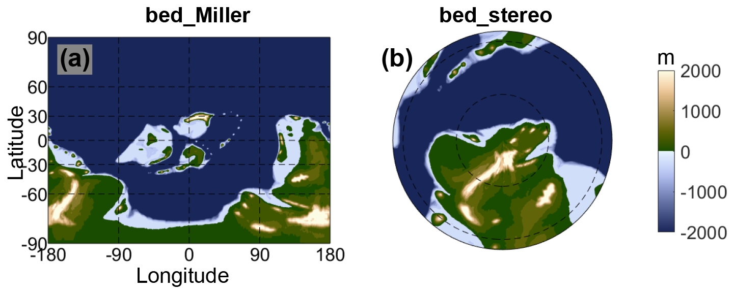
Figure 1 Late Ordovician palaeogeography. (a) Late Ordovician palaeogeography under the Miller projection. (b) as (a), but with a stereographic projection centered at the South Pole.

2.2 Ice sheet model

The simulations of continental ice sheet were performed using the Ice-sheet and Sea-level System Model version 4.23 (ISSM 4.23), jointly developed by NASA Jet Propulsion Laboratory (JPL) and the University of California, Irvine (UCI) (Larour et al., 2012). ISSM is a finite-element, thermo-mechanically coupled ice sheet model that solves the mass, momentum, and energy balance equations on an unstructured mesh. In this study, the model is configured at a horizontal resolution of 60 km with 15 vertical levels, and the dynamical core is based on the Shallow Ice Approximation (SIA). The basal melt rate beneath floating ice shelves is prescribed at 0.1 m yr⁻¹, within the range commonly adopted in previous Antarctic ice sheet studies (Pollard and DeConto, 2012).

ISSM uses monthly mean surface temperature and precipitation from the CESM simulations to calculate surface mass balance. Surface accumulation is directly derived from the frozen fraction of precipitation, while ablation is calculated using the Positive Degree-Day (PDD) method (see more details in Appendix A), and superimposed ice formation is represented by a parameterization scheme. In all PDD-based calculations, a standard deviation (σ) of 5.5 °C is applied to account for monthly air temperature variability (Reeh, 1991). The PDD approach assumes that near-surface air temperature controls melt processes through an empirical relationship with the melting point. Despite its simplicity, this scheme has been demonstrated to reproduce large-scale ice sheet behaviour effectively and efficiently (Hanna et al., 2011; Reeh, 1991; Wake and Marshall, 2015). For the basal friction formulation, the Paterson-type sliding law is employed, with parameter values calibrated to best reproduce modern Antarctic ice volume and flow patterns (Man et al., 2023).

2.3 Asynchronous coupling between the climate and ice sheet models

An asynchronous coupling strategy (Wei et al., 2023) was employed to link the climate model (CESM) and the ice sheet model (ISSM). In this approach, CESM and ISSM exchange boundary conditions at discrete coupling intervals, allowing each model to evolve independently over its characteristic timescale. During each coupling cycle, surface elevation and surface type in CESM (e.g., transitions among vegetation, bare ground, wetlands, and glaciers) are updated according to the evolving ice sheet geometry and extent. Conversely, ISSM is forced by monthly mean surface temperature and precipitation fields from CESM to perform thermo-mechanical and dynamical simulations of ice sheet growth and retreat. The simulations are initialized from the CTRL, and the ice sheet model evolves from an ice-free initial state to equilibrium conditions. The coupling frequency is designed such that the ratio of climate to ice sheet model time steps is approximately 10 : 2500, corresponding to one coupling exchange every 10 CESM years, during which ISSM integrates independently for 2500 model years. The total integration time of the ice sheet model is 200 ka (i.e., eighty coupling cycles). After the coupled ice sheet reached its equilibrium state, the climate model was further integrated for an additional 1000 years to allow the deep ocean to approach a steady state. Equilibrium is diagnosed based on the stabilization of global mean top-of-atmosphere (TOA) net radiation (< 0.1 W m⁻²) and GMST (the trend of drifting < 0.2 °C during the final 100 years) in CESM, together with changes in ice sheet extent and thickness (< 1 % during the last coupling interval) simulated by ISSM. The equilibrium state and selected intermediate snapshots are subsequently analyzed to investigate the coupled climate–ice sheet interactions.

2.4 Experiments

In previous uncoupled ice sheet-climate simulations, the feedback of ice sheet to climate was normally considered by simply adjusting temperature and precipitation forcings by lapse rate and glacial desertification effects, respectively, which then affect ice sheet growth and evolution (Herrmann et al., 2004; Vizcaíno et al., 2010). While this method of forcing can partially reflect the impact of ice sheet on the local climate, it does not fully capture the feedback between the cryosphere's evolution and the other components of the Earth system. For comparison with such a traditional method, we first run an offline ice sheet simulation using the equilibrium results from the climate model under pCO₂ of 6 PAL (case OFFLINE). Then, a coupled simulation is carried out under the same CO₂ level. In the coupled simulation, the evolution of ice sheet affects surface topography, albedo, and atmospheric and oceanic circulations. These changes, in turn, modify the temperature and precipitation fields that drive ice sheet growth, thereby regulating its stability and expansion (case CP). We have also performed a supplementary coupled experiment, where we disabled the “land surface type feedback” by repeating the asynchronously coupled simulations without surface type change (case CP_NO_ALB; the ice-sheet area was set to 0 during coupling). By doing so, we will be able to assess the relative contributions of albedo and topography changes to the simulation results when coupling to the ice sheet models.

To further isolate the respective roles of the ocean and atmosphere in mediating the climatic impact of the ice sheet, two additional sets of experiments are carried out. In one of them, global SST is prescribed to that of the CTRL, while in the other, the ocean is run in a slab ocean mode (SOM). In the SOM experiments, the ocean heat transport is also prescribed as in the CTRL. Each set was performed with a large continental ice sheet obtained from the equilibrium state of the fully coupled simulation and fixed throughout. The prescribed-SST simulations allow us to extract the direct influence of ice sheet on atmospheric circulation (case FIXED_SST), while the SOM simulations allow us to distinguish between the contributions of ocean heat transport and surface heat exchange to the temperature anomalies observed in the fully coupled experiment (case NO_DYN_OCN).

To isolate the respective contributions of ice-sheet albedo and topography, we conducted two slab-ocean sensitivity experiments: one in which the ice-sheet albedo is prescribed at its full glacial value obtained from the case CP, but the surface topography is flattened to the ice-free condition (case ALB_ONLY), and another in which the full ice-sheet topography is imposed but the ice sheet area is kept to 0 to account for albedo changes associated with the ice sheet (case TOPO_ONLY). The contribution of ice-sheet albedo is thus diagnosed as the difference between the ALB_ONLY and CTRL, while the contribution of ice-sheet topography is diagnosed as the difference between the TOPO_ONLY and CTRL. All experiments were integrated for 300 years, and the climatological means of the last 100 years are analyzed below.

3 Results and discussion

3.1 The Late Ordovician ice sheet

In the offline simulation where ice sheet-climate feedbacks are not considered, the results align with those of previous studies (Herrmann et al., 2004; Lowry et al., 2014; Pohl et al., 2016): the ice sheet is confined to high-latitude regions (≥ 60° S), showing significant discrepancies with the geological tillite records (Cocks and Torsvik, 2021) (Fig. 2). And our case CTRL yields a tropical SST of 28.2 °C, which is in close agreement with the conodont oxygen-isotope-based reconstruction of Trotter et al. (2008). Furthermore, our pCO₂ adjustment simulations show that Arctic sea ice is widespread when pCO₂ falls below 3 PAL (GMST = 13.5°C), whereas high-latitude sea ice in the Southern Hemisphere does not begin to form until pCO₂ drops to ∼ 1.5 PAL (GMST = 8 °C). Because the climate condition is comparable to that of reconstruction, the flawed results of the offline ice sheet simulation should not be primarily due to the overestimated surface temperature, but rather the failure of a one-way forcing framework to capture the cryosphere's feedback on the climate system. The comparison with the coupled simulation, discussed in the following paragraphs, will further support this view. Lowering pCO₂ might reproduce an ice sheet extent in the offline simulations that is consistent with the geological records (Pohl et al., 2016). Tests show that pCO₂ needs to be lowered to ∼ 1.5 PAL (Fig. C1) with the corresponding GMST lowered to ∼ 8 °C, which is far lower than that of the reconstructions (∼ 15 °C) (Li et al., 2022; Scotese et al., 2021; Trotter et al., 2008). Therefore, this approach contradicts the geological constraints on both pCO₂ levels and GMST for the Late Ordovician, in which a massive continental ice sheet formed under a relatively warm climate.

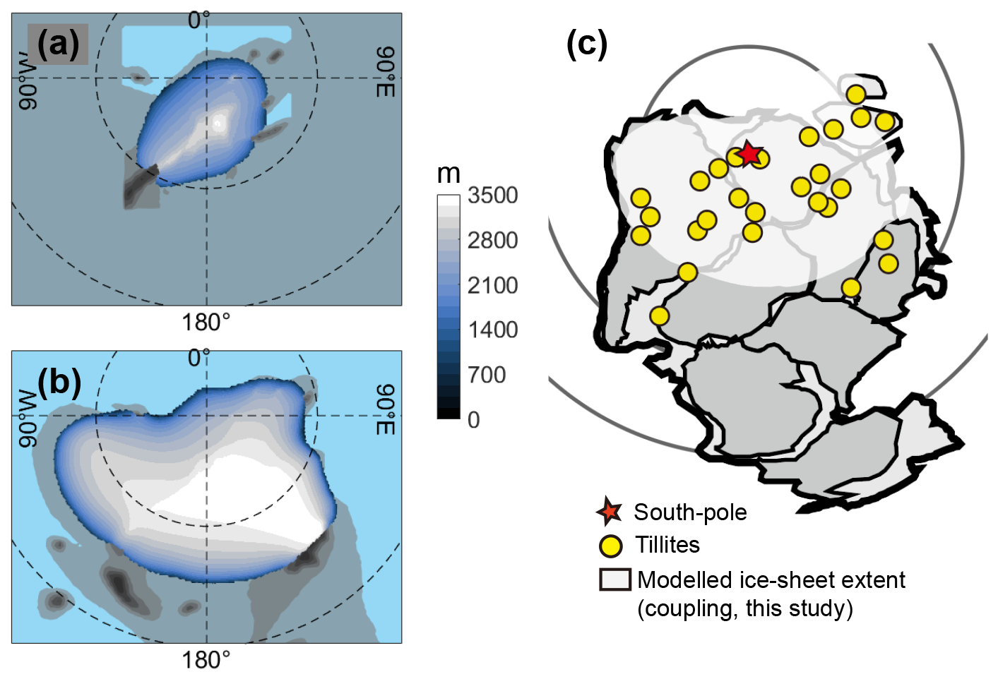
Figure 2 Late Ordovician glacial tillites and ice sheet surface. (a) Equilibrium result of the ice sheet surface topography (blue-grey color) simulated by the offline method at 6 PAL. The bedrock topography is indicated by a greyscale whose colorbar is not shown here but more details can be found in Fig. 1. (b) as in (a), but with coupled climate and ice sheet models. Latitude is shown at 30° intervals. (c) Locations of glacial deposits (Cocks and Torsvik, 2021).

Figure 2b shows the surface topography of the ice sheet in the coupled simulation at equilibrium. Compared to the uncoupled scenario, the ice sheet not only forms along the Antarctic mountain range but also extends significantly toward lower latitudes (∼ 40° S), nearly covering the entire southern portion of Gondwana. This result is broadly consistent with the general distribution of glacial tillites in the geological record, although the simulated ice sheet does not extend as far as ∼ 30° S in some regions, as suggested by some Hirnantian glaciation sedimentary records (Cocks and Torsvik, 2021; Pohl et al., 2016) (Fig. 2c). This suggests that considering ice-climate feedback is crucial for realistically reproducing the formation and distribution of large-scale ice sheet during the relatively warm Late Ordovician.

While many studies suggest that the grounded ice sheet likely connected into a whole massive ice sheet during the peak of the Hirnantian glaciation (the “large scenario”), the hypothesis of disconnected ice sheet (the “small scenario”) has still garnered support in some research (Finnegan et al., 2011). Consistent with much of the modelling work, our results support the idea that a single, large ice sheet covered the entire mid- to high-latitude supercontinent during the Late Ordovician glaciation. The total volume of the ice sheet (∼ 9.0 × 10¹⁶ m³) obtained here corresponds to a sea level drop of ∼ 210 m, comparable to the levels during the LGM (Montañez and Poulsen, 2013), which is consistent with previous reconstructions (Bergmann et al., 2025; Cocks and Torsvik, 2021). The equivalent sea-level drop is estimated by dividing the total ice volume by the global ocean surface area and we must acknowledge that this sea-level drop estimate does not account for isostatic adjustments and therefore carries uncertainties.

Most previous modelling studies of Late Ordovician continental glaciation used the offline method (Crowley et al., 1987; Crowley and Baum, 1991, 1995; Herrmann et al., 2004; Horton et al., 2007; Lowry et al., 2014; Pohl et al., 2016, 2021; Vandenbroucke et al., 2009), with Pohl et al. (2016) being the only one that did coupled simulations. Offline simulations generally needed quite low pCO₂ to produce an ice sheet comparable to the reconstructions. For example, the simulated ice sheet remained largely confined within the polar circle in Lowry et al. (2014) even at pCO₂ as low as 2 PAL. Pohl et al. (2016) did both offline and coupled simulations, using climate and ice-sheet models distinct from those used in this study. In their simulations, a sufficiently large ice sheet could not be obtained in the offline mode until pCO₂ was dropped to 3 PAL while it could be obtained in the coupled mode when pCO₂ was as high as 12 PAL. Our results of the offline experiment at 6 PAL are most comparable in areal coverage to their 10 PAL offline simulation, possibly due to differences in boundary conditions (e.g., topography, land-sea configuration, vegetation cover) and model structure. Thus, our results are broadly consistent with those of Pohl et al. (2016). However, Pohl et al. (2016) did not explicitly analyze the feedback mechanisms through which coupling facilitates ice-sheet growth. Identifying and quantifying these processes is a primary objective of the present study and is addressed in the following sections.

3.2 Limiting factors for ice sheet growth

The process of ice sheet development shown in Fig. 3g–i indicates that during the initial stage of ice sheet expansion, a small, elongated land-based ice sheet first forms, extending roughly from 80 to 60° S, along the mountain range at the southern end of Gondwana (Fig. 1). The presence of the mountains lowers the surface temperature and facilitates the initial growth of the ice sheet. The ice sheet expands to an extent similar to the equilibrium state of the offline simulation (Fig. 2a) in approximately 10 ka. Subsequently, the ice sheet grows outward from the mountain range, gradually expanding toward the continental margins and the low-latitude interior of the supercontinent, eventually reaching approximately 40° S, almost completely covering the southern portion of Gondwana. The overall shape of the ice sheet is dome-like, centered on the interior of the supercontinent, constrained by continental boundaries in the high latitudes and the 40° S line in the mid-latitude continental interior. Notably, in our simulation with pCO₂ = 6 PAL, large ice shelves do not form in any of the time periods, even around the high-latitude polar seas. This coincides with the absence of large-scale sea ice. Our configuration is consistent with the earlier results of Pohl et al. (2016), but contrasts markedly with Lowry et al. (2014), in which ice sheets flow from the coast toward the continental interior, with the highest elevation located near the coastline. Importantly, the coastal-to-interior flow pattern obtained by Lowry et al. (2014) is at odds with the glacial sedimentary record. Lowry et al. (2014) acknowledged this discrepancy in their discussion, noting that their application of uniform topography likely contributed to this pattern, as the absence of elevated interior regions removes the effect of lapse-rate cooling that would otherwise favor ice accumulation. Moreover, high topography can also act as an ice nucleation center and modify atmospheric heat transport and precipitation through its influence on stationary wave patterns. This suggests that the inclusion of realistic surface elevation is essential for accurately capturing ice sheet geometry.

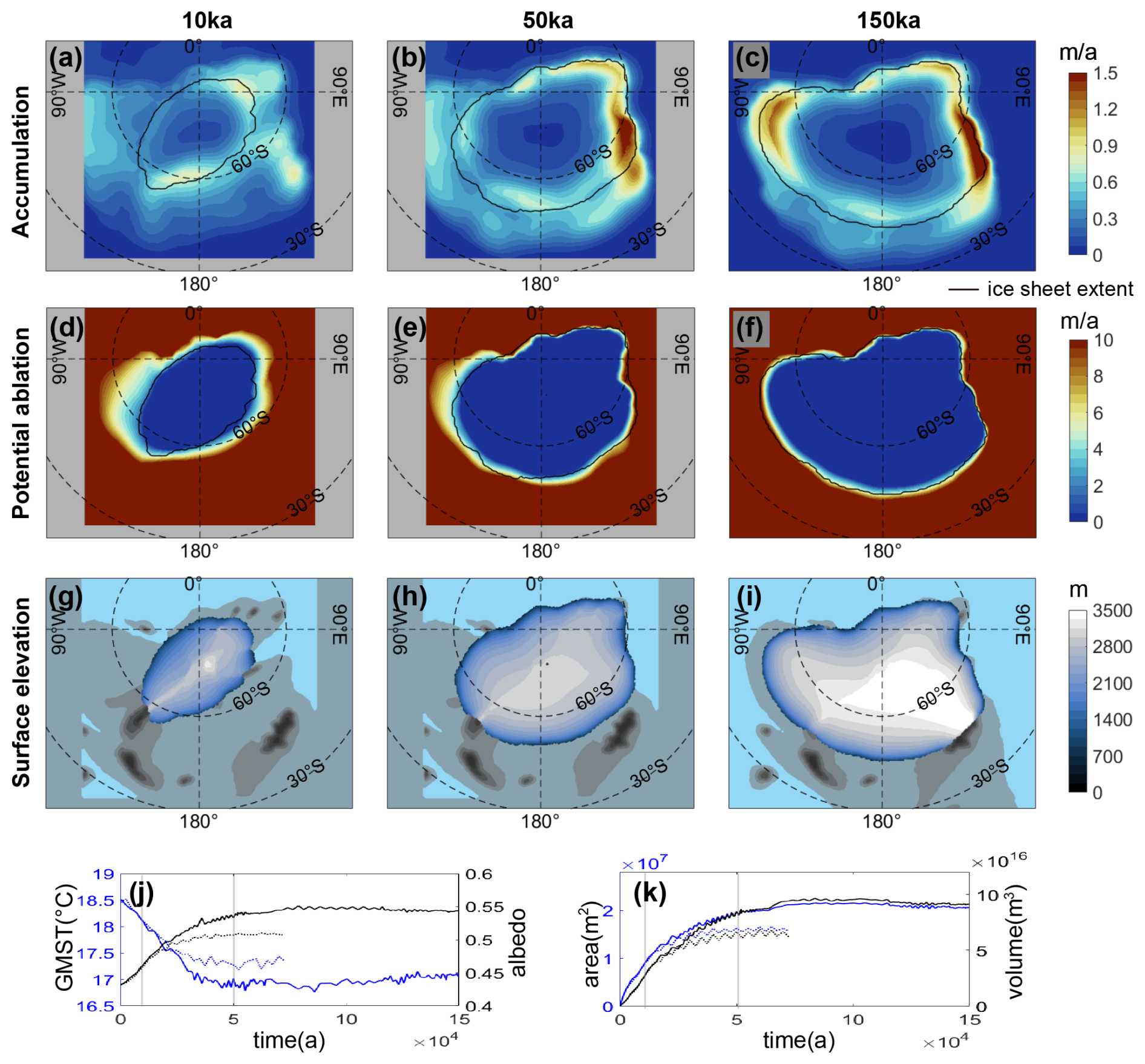
Figure 3 Contribution of accumulation and ablation to ice sheet growth. Three snapshots from the coupled framework simulation (CP) at (a, d, g) 10 ka, (b, e, h) 50 ka, and (c, f, i) 150 ka. The rows from top to bottom show accumulation, potential ablation, and surface elevation of the ice sheet, and the corresponding time series. In particular, when displaying time series, the left panel shows the evolution of GMST (°C; blue) and global annual mean land surface albedo (black), and the right panel shows ice-sheet area (m²; blue) and ice-sheet volume (m³; black). Solid lines show the fully coupled experiment (CP), while dashed lines show the supplementary experiment in which the ice-sheet area was set to 0 during coupling (CP_NO_ALB). The black contour represents the ice-sheet edge. Latitude is shown at 30° intervals.

Inspection of glacier dynamics suggests that precipitation was not the limiting factor for the growth of the land-based ice sheet during the Late Ordovician glaciation (Fig. 3a–c), unlike that for the Tibetan Plateau during the LGM (Wei et al., 2023). In fact, during the development of the ice sheet, precipitation was almost never lacking over the growth zone near the ice sheet front (Fig. C3). This is probably because the mid-latitude moisture transport was powerful under a relatively warm climate state while the mountain range was neither high nor extensive enough for its blocking effect to substantially cut off the moisture supply. For the Late Ordovician, it is the high temperature that is preventing the ice sheet from expanding in the offline simulation (Fig. 3a).

The CP time series (solid lines) of Fig. 3j show a rapid adjustment of the ice sheet-climate system during the early stage of the experiment, followed by a gradual approach to equilibrium. GMST decreases sharply from about 18.5 to 17.1 °C within the first ∼ 30 ka, while the global annual mean land surface albedo increases from 0.43 to 0.55 over a similar timescale. After ∼ 50 ka, both GMST and albedo vary weakly, indicating that the climate state has largely stabilized. The ice-sheet area and volume show a corresponding growth pattern (Fig. 3k). Both increase rapidly during the first 30 ka. After ∼ 80 ka, the ice sheet enters an equilibrium state, with only small fluctuations thereafter.

A key feature is the strong temporal correspondence between albedo increase and ice-sheet growth. The rapid rise in albedo occurs during the same interval as the fastest expansion of ice-sheet area and volume, while the subsequent stabilization of albedo coincides with the slowdown of ice-sheet growth. This suggests that surface albedo exerts a critical control on ice-sheet development through the ice-albedo feedback: as the ice-covered area expands, surface reflectivity increases, reducing absorbed radiation, cooling the surface, and further promoting ice accumulation. The close coupling among increasing albedo, declining GMST, and expanding ice volume indicates that ice-albedo feedback is a key mechanism controlling both the transient growth phase and the eventual quasi-equilibrium size of the ice sheet. In our coupled simulation, the growth of an ice sheet increases the surface albedo and lowers the temperature of the surrounding region, expanding the region of low ablation (compare the low-ablation zone to the ice edge (black curve) in Fig. 3d–f). As the ice sheet expands, the low-ablation region also extends outwards, until the ice sheet reaches low enough latitudes (∼ 40° S), where the temperature is too high so that the ablation remains high even right at the edge of the ice sheet (Fig. 3f).

We have also performed a supplementary coupled experiment, in which we repeated the asynchronously coupled simulations without surface type change (CP_NO_ALB, dashed lines in Fig. 3j, k). The results were revealing. The absence of albedo change reduces the final extent of land-ice expansion, confirming its important role. Nevertheless, substantial land-ice growth still occurred. The growth of this portion of the ice sheet can be understood as a result of the ice sheet topographic uplift: as the ice sheet surface elevates, temperatures decrease and effectively suppress ablation; simultaneously, the towering ice sheet topography drives strong downslope katabatic winds (as discussed in detail in the following sections), transporting cold air from the summit to the margins, lowering marginal temperatures to further suppress ablation; last but not least, the elevated, low-temperature environment leads to an expansion of snow cover in the climate model (not shown), in which case the snowfall process built in to the CESM and associated snow-albedo feedback partially compensates for the lack of ice-albedo feedback. As a result, we believe that here, at least during such a supercontinental period, topographic feedback is also very important, even more important than the ice-albedo feedback (note that we are not referring to the overall snow-ice-albedo feedback here, because we can not rule out snow-albedo feedback in the simulations).

Taken together, the results of CP and CP_NO_ALB lead us to conclude that it is the combined effect of albedo and topography that supports ice sheet growth in the coupled simulation. In particular, the contribution of topography to continental ice sheet formation cannot be overstated.

3.3 The katabatic winds

In addition to the primary ice albedo feedback, the katabatic winds, which blow downslope along the ice sheet's surface, also play a significant role. The katabatic wind is a gravity-driven cold air advection phenomenon that is commonly observed in polar and mountainous regions (Parish and Cassano, 2003; Vihma et al., 2011), such as Antarctica, the Greenland ice sheet, and the Alps. Taking Antarctica as an example, the long polar night causes the surface to cool continuously, dramatically lowering near-surface air temperatures and creating a stable cold air layer (Connolley, 1996). Due to the high elevation and steep slopes near its edges, cold air accelerates downslope under gravity, with wind speeds sometimes exceeding 50 m s⁻¹.

In our coupled simulation of the Late Ordovician glaciation, strong katabatic winds begin to form as the ice sheet grows (Fig. 4e–h). When there is no ice sheet, the cold polar air mainly blows towards the ocean between 90° W and 0° E (Fig. 4a–d), especially in the austral winter, while warm air blows polewards in the summer at certain locations on the continents (e.g., between 135 and 180° W). This warm air advection will prevent the ice sheet from growing in the offline simulation. In the coupled simulation, however, once an ice sheet is present, the cold air blows towards the continental interior in both winter and summer, expanding the low-temperature (< 0 °C) region (compare Fig. 4e, i to a). Ice-sheet formation thus leads to a fundamental reorganization of regional atmospheric circulation, marked by the development of strong katabatic winds. Cooling and densification of air over the cold ice-sheet surface allow dense air to drain downslope from the ice-sheet interior toward the surrounding lowland area, generating cold, gravity-driven near-surface flows. This enhanced cold air helps increase snow accumulation during winter and spring, and reduce ablation during summer around the ice sheet's edges.

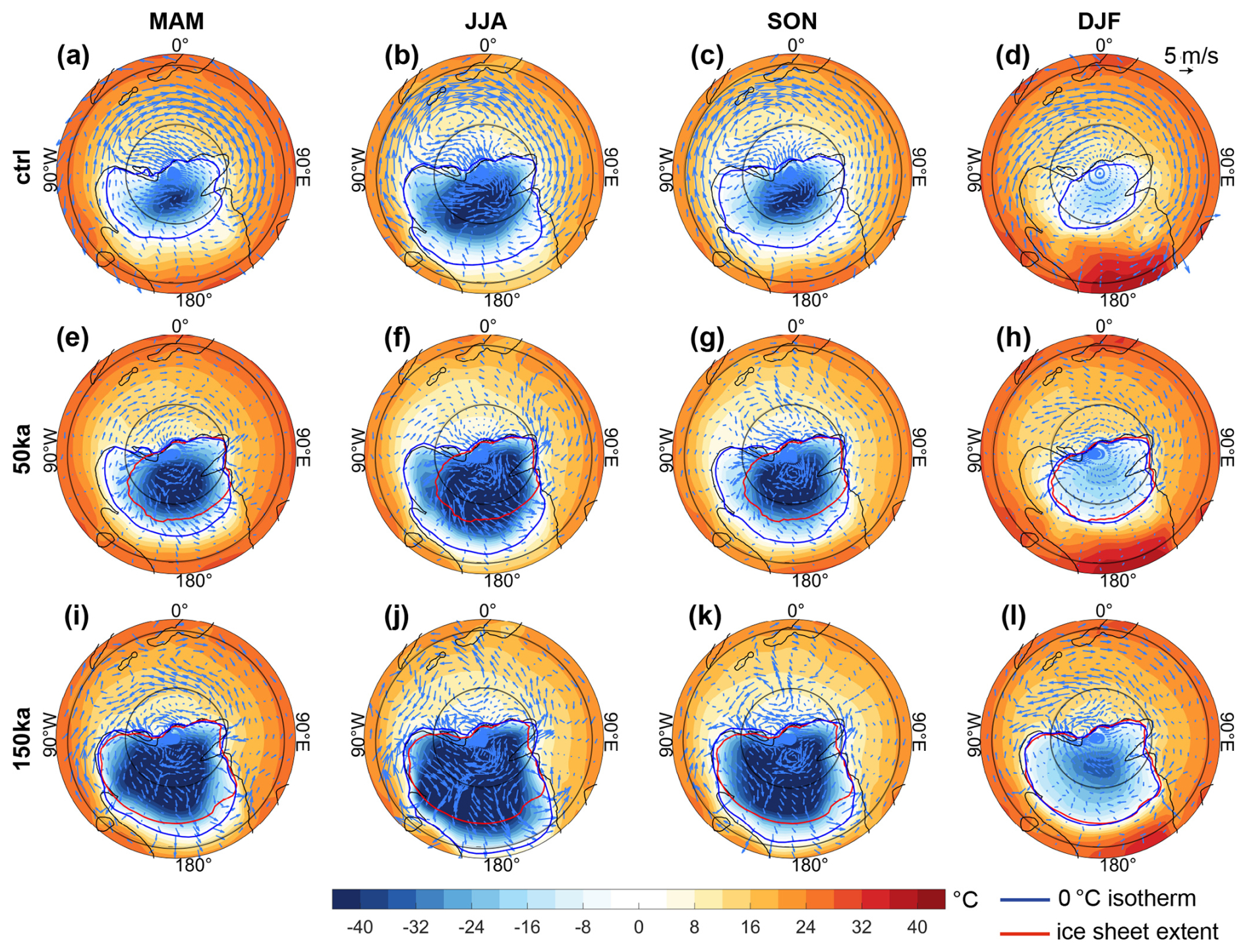
Figure 4 Surface wind field and temperature. (a–d) Surface wind field and surface temperature from the equilibrium of the CTRL for March, April, May (MAM); austral winter (June, July, and August; JJA); September, October, November (SON); and austral summer (December, January, and February; DJF). Two snapshots from the coupled framework simulation are shown in (e–h) 50 ka, (i–l) 150 ka. Note that in (e–h) and (i–l), the surface wind is shown as the difference from the CTRL. The 0 °C isotherm and ice-sheet extent are indicated by the blue and red contours, respectively. Latitude is shown at 30° intervals.

When the ice sheet expands to ∼ 42° S (red curves in Fig. 4i–l), the katabatic winds remain strong in austral winter, but become negligible in summer. The high summer ablation at mid-latitudes prevents the ice sheet from further expanding. This seasonal asymmetry reflects a fundamental shift in the near-surface thermal and dynamical controls on the flows. During summer, increased solar heating warms the mid-latitude ice-sheet surface and the overlying boundary-layer air, eroding the strong surface cooling that drives cold air downslope drainage. As a result, the gravity-driven cold air advection along the ice-sheet slopes is greatly reduced in austral summer. And as the ice sheet expands, the ice front reaches sufficiently low latitudes, where the surface temperatures sustain high ablation rates. Under such conditions, the enhanced melt counteracts further margin advance, consistent with the negative feedback mechanism described earlier, in which ice-sheet expansion into ablation-prone zones can offset mass gain and finally stabilize the ice sheet. The strong mid-latitude temperature gradient thus could play a key role in stabilizing the land-ice front. This result highlights the positive feedback mechanism of “ice sheet growth – katabatic winds of cold air advection – continued ice sheet growth” during the Late Ordovician, providing a clear dynamic explanation for the rapid expansion of the ice sheet during this period.

3.4 Equilibrium climate change due to ice sheet

Figure 5 shows the surface temperature and ocean surface currents from CTRL, the temperature differences between NO_DYN_OCN and CTRL, and the differences in surface temperature and ocean surface currents between CP and CTRL. In the land-ice-free case CTRL, the land is much colder than the oceans during the austral winter (Fig. 5a), partially because of the presence of snow and associated high surface albedo (not shown). The seasonal cycle of the surface temperature over land is much stronger than over oceans (compare Fig. 5b and a). Because the majority of the continent is located in the mid- to high-latitude region of the SH, this hemisphere exhibits stronger seasonal variations and colder annual mean surface temperature than the Northern Hemisphere (NH).

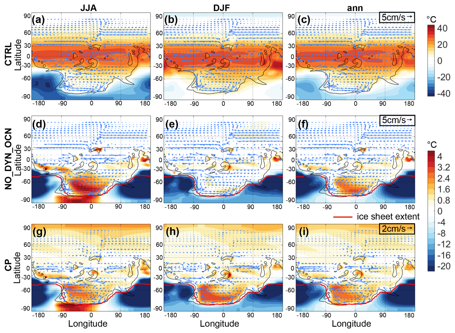
Figure 5 Surface temperature and ocean surface currents. (a–c) Surface temperature and ocean surface currents (averaged over the upper 200 m) from the CTRL for austral summer (DJF), winter (JJA), and annual means. (d–f) Temperature differences between the slab ocean case NO_DYN_OCN and CTRL, with the ocean currents of the CTRL superimposed. (g–i) The difference in surface temperature and ocean surface currents between the CP and CTRL. Note that the color scale is different when showing positive and negative temperature differences.

Surprisingly, surface temperature increases in many regions when a large ice sheet grows. These regions include tropical lands, the global ocean, and even the ice sheet in a small region around the South Pole (Fig. 5g–i). The increase in local temperature can exceed 4 °C in some areas. The results of SOM experiments (and prescribed-SST experiments as will be shown later) indicate that the SH ocean warming as well as the warming over tropical lands is primarily driven by atmospheric processes (Fig. 5d–f), while the NH ocean warming is mainly triggered by oceanic processes (compare Fig. 5g–i to d–f).

The warming over the high-latitude SH ocean is due to the strengthening of a stationary wave between 30 and 60° S when a large ice sheet develops. This stationary wave has a wavenumber-1 structure as evidenced by the 500 hPa eddy geopotential height field (Fig. 6). In the CTRL, the high- and low-pressure anomalies are located over the windward and leeward sides of mountain range, respectively (Fig. 6a–c), very similar to what happens near the Rockies and Tibetan Plateau of the present day (Held et al., 2002; Lee et al., 2023). The two nodal points – where pressure anomalies are zero – are located at the middles of the ocean and continent, respectively. The one in the middle of the ocean guides warm low-latitude air into the high-latitude region, while the one in the middle of the continent guides cold high-latitude air into the low-latitude region.

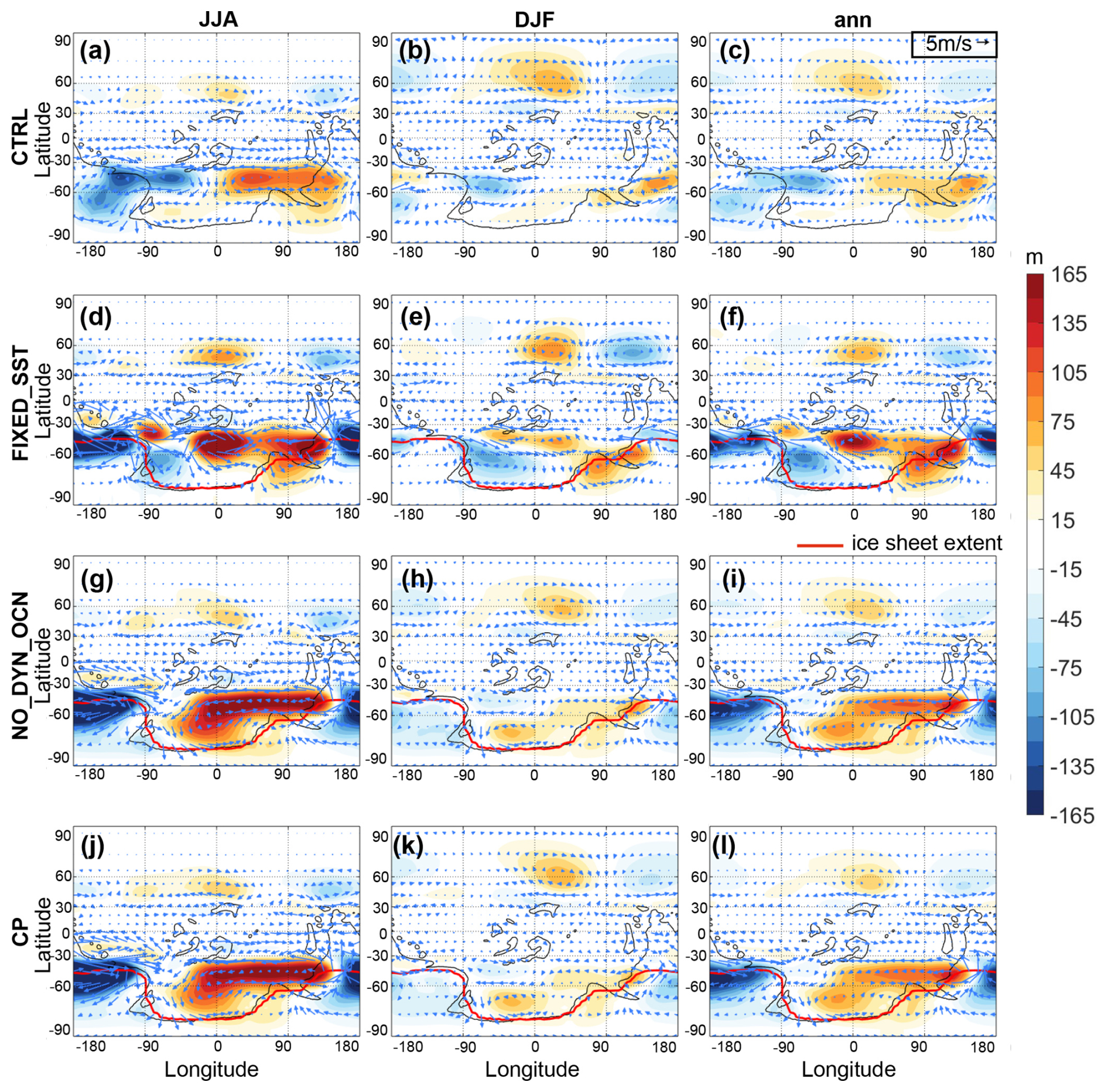
Figure 6 Structure of the stationary waves. (a–c) 500 hPa geopotential height and wind field from the CTRL, with zonal average subtracted. (d–f) as (a–c), but for the prescribed-SST experiment results. And (g–i) for the case NO_DYN_OCN, (j–l) for the coupled experiment.

When a large ice sheet develops on the continent, the SH stationary wave is substantially strengthened (Fig. 6d–l), especially during the austral winter, enhancing atmospheric heat transport towards the high latitudes over the ocean region (Fig. 7). This strengthening happens in the prescribed-SST experiment (Fig. 6d–f), indicating a primary influence of the ice sheet on the atmospheric circulation. Along with the strengthening, the phase of the stationary wave shifts westwards by about 30° longitude. Both the strengthening and westward shift of the wave are likely due to the enhanced blocking of the westerly wind by the high topography of ice sheet and the westward shift of ice edges (compare Fig. 2a and b). The southward transport of warm air with a temperature anomaly of 3–4 °C across 65° S at the nodal point (∼ 60° W) is clearly demonstrated in Fig. 7.

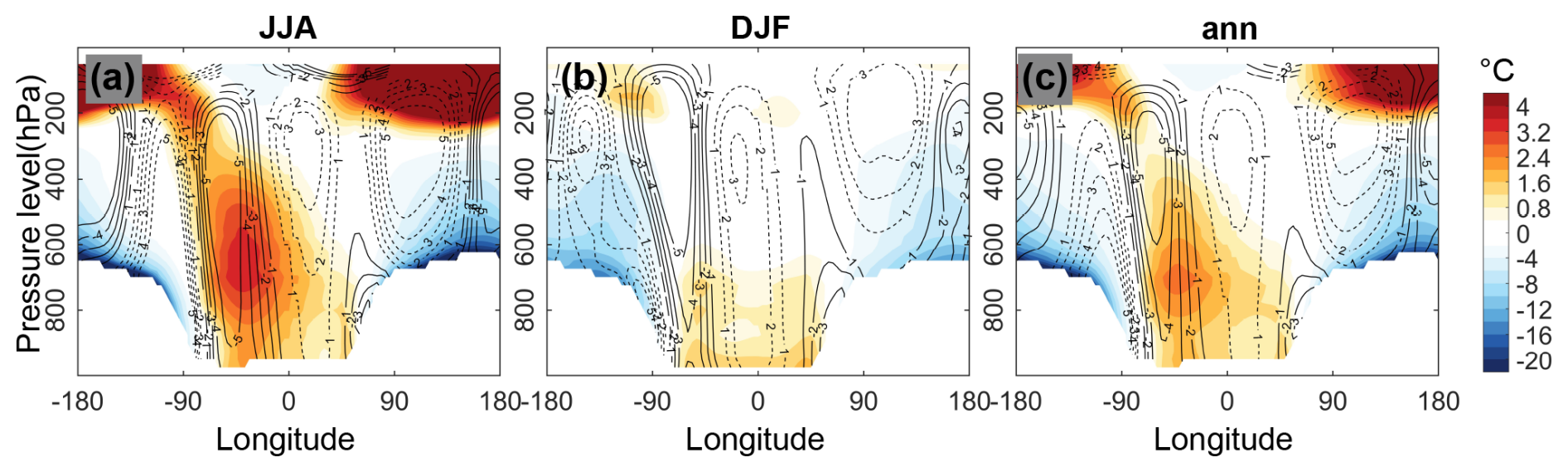
Figure 7 Difference in air temperature (color shading) and meridional wind (contours) along 65° S between the coupled and the control experiments. Solid and dashed contours indicate northerly and southerly wind anomalies, respectively. Note that the color scale is different when showing positive and negative temperature differences.

When the SST is allowed to change (as in the case NO_DYN_OCN), the pattern of this stationary wave is slightly modified and extends more poleward (compare Fig. 6d–f to g–i), enabling atmospheric heat transport towards even higher latitudes. Note that sea ice plays a negligible role in this change because it is nearly absent even during the austral winter. This pattern remains almost the same when the ocean dynamics are turned on (as in the coupled ice-climate simulation; compare Fig. 6g–i to j–l) but the surface ocean current also helps transport more heat to the high-latitude region (Fig. 5g–i). Due to the strengthening of the high-pressure anomaly over the oceanic region, the clouds and the associated negative radiative forcing are reduced (Fig. 8d–f; the net effect of reduced shortwave cloud radiative forcing results in net energy gain at the surface), also having a warming effect. In any case, the results highlight the importance of the atmospheric process in driving the warming over the mid- to high-latitude oceanic region.

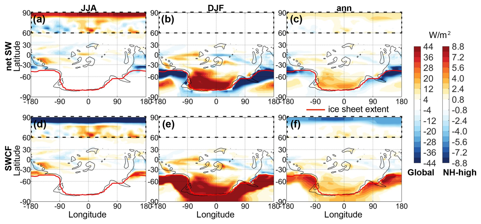
Figure 8 The differences in (a–c) net surface shortwave radiation and (d–f) shortwave cloud radiative forcing between the coupled and the control experiments. Note that the color range for high latitudes in the NH (black dashed box) has been adjusted, as the radiation changes in the NH are relatively minor.

The warming over different tropical lands in the coupled simulations relative to the control is due to different reasons. For islands, the primary reason is the reduced clouds and associated blocking effect on solar radiation (Fig. 8). For the tail of the supercontinent extruding into the tropical region, the warming is caused by the changes in the hydrological regime, as confirmed by the net precipitation and latent heat flux anomalies in this region (not shown).

The NH warming does not appear in the SOM simulation, indicating a primary role of ocean dynamics. The changes in both the deep meridional overturning circulation (MOC) and the subtropical cell (STC) could play a role. As the SH polar ocean warms, the deepwater formation there weakens, so does the MOC (Fig. 9). In the meantime, the STC of the SH becomes shallower (Fig. 9). Meanwhile, the decrease in SH deep-water formation (Fig. 9) provides no explanation for the regional ocean warming – which would require an increase in deep-water formation – further pointing towards a driving role of atmospheric processes in the coupled model. The weakening of this anti-clockwise MOC and shallowing of STC should reduce the southward heat transport across the equator and warm the NH. It's worth noting that our ice sheet coupled simulation shows weak influence on the MOC, with no northern-sourced deep water formation before or after ice-sheet inception. In contrast, previous studies have demonstrated that changes in pCO₂ and solar constant exert a far stronger impact on ocean circulation (Pohl et al., 2016).

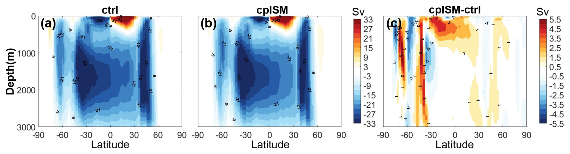
Figure 9 Oceanic meridional overturning circulation. Panels show the ocean meridional overturning streamfunction for (a) case CTRL, (b) case CP and (c) the difference (CP minus CTRL). Negative values indicate counterclockwise circulation.

The change of oceanic heat transport confirms that less (∼ 0.08 PW; 1 PW = 10¹⁵ W) heat is transported southward across the equator and more heat is transported towards the NH by the ocean when a large ice sheet develops (blue curves in Fig. 10). While the atmospheric heat transport remains almost the same at the equator (red curves in Fig. 10), making the total heat transport (black curves in Fig. 10) towards the NH increase. Note that the oceanic and total heat transport towards the NH high-latitude region decreases in the ice sheet-climate coupled simulation compared with the control simulation. This is because the results shown in Fig. 10 are for the equilibrium states, at which the NH polar region has already warmed (Fig. 5g–i). At the beginning of the coupled simulation, the oceanic heat transport does increase in the NH high latitudes, reducing the sea ice there. In the latter stage, the reduced sea ice (not shown) and thus increased absorption of solar radiation (Fig. 8) sustain the warming there.

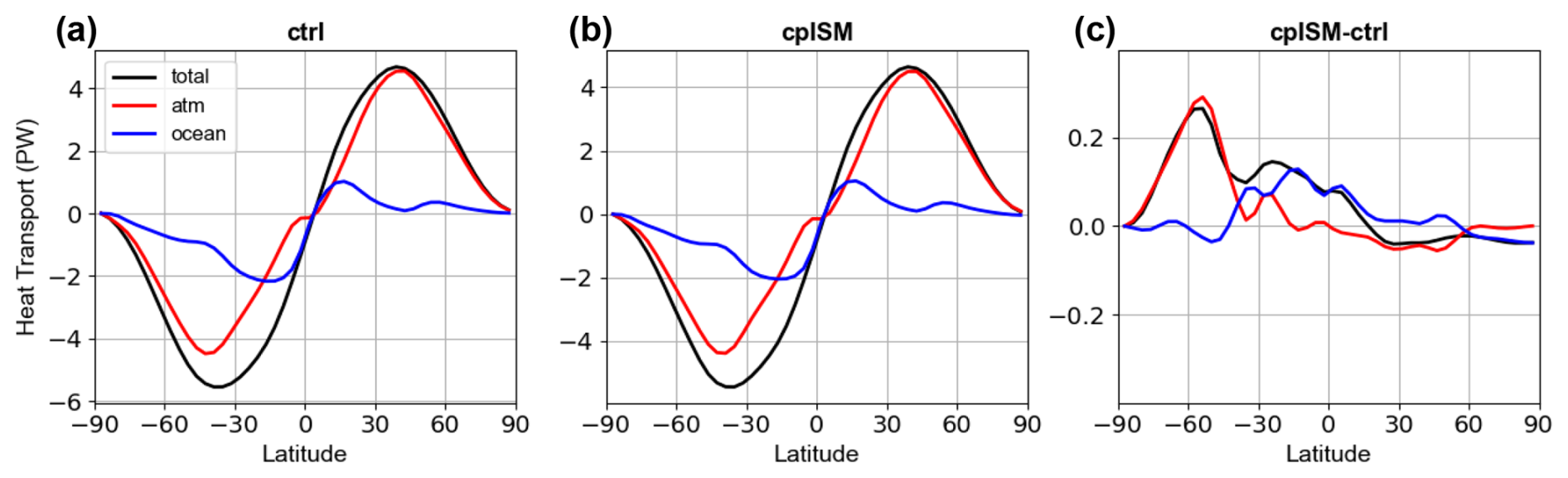
Figure 10 Simulated meridional heat transport. Panels show the total, atmospheric, and oceanic contributions to the meridional heat transport. (a) case CTRL, (b) case CP and (c) the difference (CP minus CTRL). Positive values indicate northward heat transport.

To further evaluate the potential imprint of land-ice growth on low-latitude geochemical records, we calculated the expected changes in surface seawater oxygen isotope (δ¹⁸O_w) and apatite oxygen isotope (δ¹⁸O_apatite) from the simulated SST and SSS fields (Fig. B1). The two low-latitude regions correspond to possible Ordovician oxygen-isotope records from Laurentia, including the Anticosti Island region, and Gondwana, including Australia, respectively (Trotter et al., 2008). In both regions, coupling to the ice sheet produces only a small SST change (Fig. B1c), consistent with the weak tropical temperature response discussed in the main text.

3.5 Relative contributions of ice sheet topography and albedo

To isolate the respective contributions of ice-sheet albedo and topography, we conducted two SOM experiments: one with the full glacial albedo but ice-free topography (ALB_ONLY), and another with full glacial topography but zero ice-sheet area (TOPO_ONLY). Similar to the analysis in the previous section, the topographic forcing emerges as the primary contributor to the warming of the SH oceans in our simulations. The elevated ice sheet acts as a mechanical barrier to the atmospheric flow, generating a stationary wave pattern. The ALB_ONLY experiment, in contrast, produces a modest temperature response over the land ice covered region, suggesting that the radiative effect of ice albedo is largely confined to the ice-sheet region itself, although some very weak cooling occurs in other parts of the world.

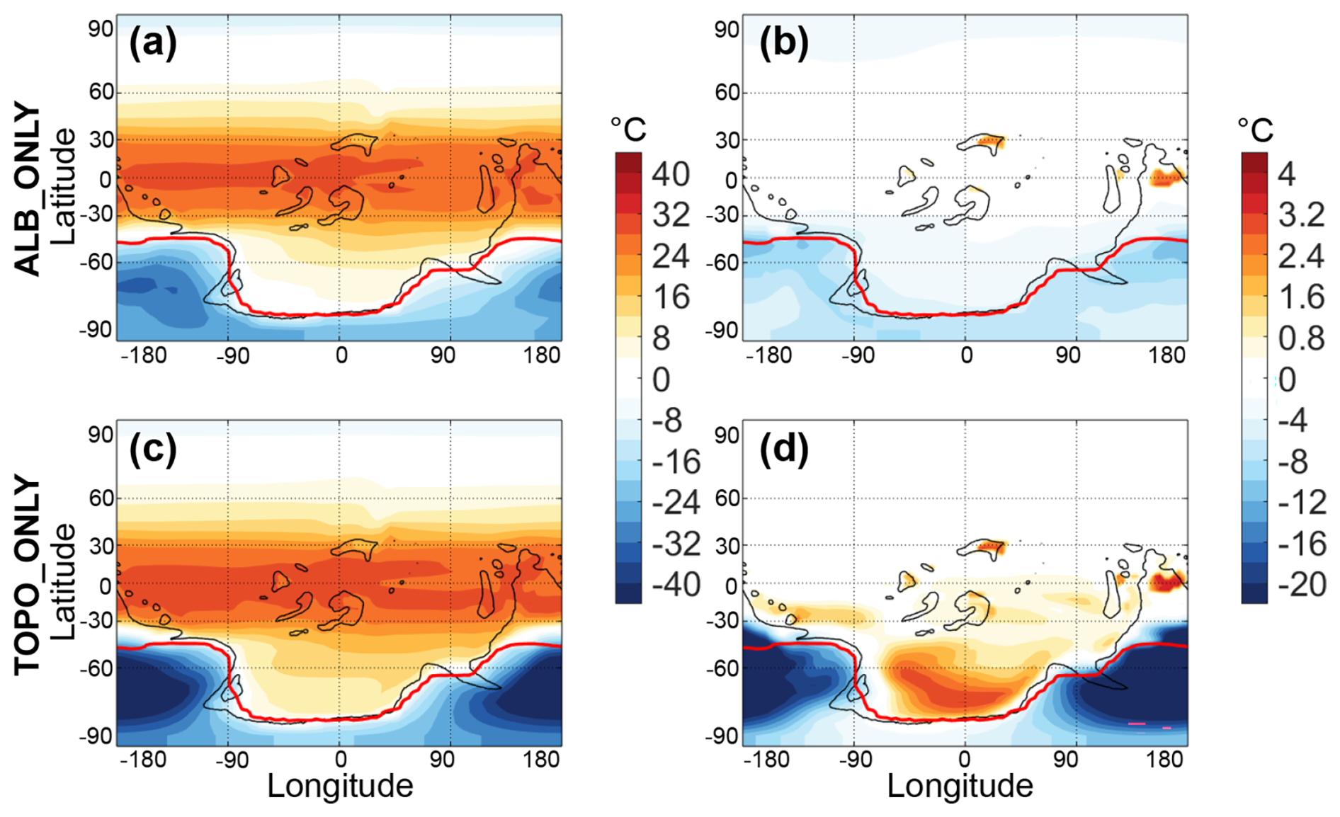
Figure 11 Surface temperature responses in the slab-ocean sensitivity experiments isolating ice-sheet albedo and topography effects. Left panels (a, c) show the annual mean surface temperature in the ALB_ONLY (a) and TOPO_ONLY (c) experiments. Right panels (b, d) show the differences relative to the CTRL, highlighting the temperature response exclusively due to ice-sheet albedo (b) and topography (d). The red contour in each panel denotes the ice-sheet margin in the full glacial configuration.

A crucial distinction must be drawn between the role of albedo during ice-sheet growth and its role in the equilibrium climate examined here. In the transient, coupled ice-sheet evolution, the ice-albedo feedback acts as the dominant positive feedback: increased ice extent raises surface albedo, which reduces absorbed shortwave radiation, further cooling the surface and promoting additional ice growth. Without this feedback, the coupled model would fail to produce an ice sheet of such magnitude (see more details in the Supplement). The more muted surface temperature response in ALB_ONLY relative to TOPO_ONLY at equilibrium therefore does not contradict the importance of albedo; rather, it indicates that once the ice sheet has reached its steady-state extent, its radiative effect may be geographically confined, whereas its topographic effect propagates globally through atmospheric dynamics.

3.6 Implication for the duration of the Ordovician continental ice sheet

One unresolved question concerns the precise time of continental ice sheet initiation and persistence during the Ordovician cooling interval. Trotter et al. (2008) used oxygen isotope (δ¹⁸O) data to outline the long-term climate evolution during the Ordovician (Fig. C4), identifying a transition from greenhouse conditions (∼ 42 °C at palaeoequator) to near-modern equatorial temperatures (∼ 28 °C) along with a rapid cooling episode during the Hirnantian. Conventional interpretations have generally suggested that mid-latitude continental ice sheet were short-lived (∼ 1 Ma) (Bergmann et al., 2025; Cocks and Torsvik, 2021; Delabroye and Vecoli, 2010; Finnegan et al., 2011), appearing only briefly during the Hirnantian. In contrast, Finnegan et al. (2011) used clumped-isotope data to argue for substantial land-based ice volumes well before the Hirnantian, potentially as early as the Katian. Meanwhile, Middle to Upper Ordovician sedimentary successions document repeated glacioeustatic fluctuations (Dabard et al., 2015; Rasmussen et al., 2016). These eustatic cycles point to the existence of continental ice sheets as early as the Darriwilian (467 Ma), rather than a sudden, Hirnantian-restricted glaciation (445–444 Ma). Furthermore, Pohl et al. (2016) provided support from coupled ice-sheet modelling simulations for a prolonged glaciation that may have begun as early as the Middle Ordovician.

Our simulations show that the initial formation and early expansion of the ice sheet have minimal impact on tropical SSTs, suggesting that the ice sheet activity may not be accompanied by global-scale cooling. On the contrary, combined with our foregoing results that the continental ice sheet induces ocean warming over SH high latitudes, it plays a crucial role in maintaining SH high-latitude ocean temperature stability, delaying its sharp cooling. This implies that the tropical SST records curve, such as those from Trotter et al. (2008), are unlikely to record major temperature shifts at high latitudes. Based on a comparison with the tropical SSTs in our coupled simulations and records, the equatorial temperatures of such a condition in our model work (a large continental ice sheet in 6 PAL) may correspond more to the Middle Ordovician.

4 Conclusions

To assess the critical role of ice sheet-climate interactions in Late Ordovician glaciation, this study conducted both uncoupled and coupled simulation experiments. The results indicate that the inclusion of bidirectional feedback between the ice sheet and the climate system is a key factor in improving the agreement between simulated outcomes and geological reconstructions. For pCO₂ (= 6 PAL) suitable for obtaining a GMST that is consistent with reconstruction (Scotese et al., 2021; Trotter et al., 2008), the uncoupled model obtains an ice sheet confined to the polar regions (≥ 60° S), contradicting the geological records. In contrast, the coupled model is able to simulate a large ice sheet that covers the southern part of Gondwana, extending to about 40° S. The results show that the growth of the Late Ordovician Gondwana ice sheet was mainly controlled by the ablation process, rather than accumulation. Our coupled simulations capture the critical feedback of ice sheet on large-scale processes such as atmospheric circulation, and accurately reproduce regional cooling processes driven by the strong ice albedo positive feedback, which provides a crucial mechanism for the substantial expansion of the ice sheet during the Late Ordovician. We then identify a key local positive feedback, that is, the “ice sheet growth – cold air advection due to katabatic winds – further ice sheet expansion”. Furthermore, no large-scale sea ice is observed in the simulation, indicating that sea ice formation is more difficult than land ice formation under these conditions.

Although the expansion of ice sheet in this time period induced cooling over the mid- to high-latitude continental region, it induced warming over all the other regions, especially over the high-latitude oceans. This warming was initiated in the SH by the enhanced poleward atmospheric heat transport, which itself was due to the enhanced wavenumber-1 stationary wave by the expansion of ice sheet. This warming was then amplified by the reduction of clouds and the warming pattern was adjusted by the oceanic heat transport. This warming then weakened the deepwater formation in the SH polar region and thus the MOC, which originally acted to transport heat from the NH to SH. The weakening of this MOC increased the northward heat transport across the equator, which reduced sea ice in the NH polar region. This latter process is eventually responsible for the warming of the NH polar region. These results highlight the complex and unintuitive responses of surface temperature, oceanic, and atmospheric responses to ice-sheet expansion during the Late Ordovician. Our simulation results suggest that the appearance of a large ice sheet warms the ocean and the impact on tropical ocean temperatures remains limited, implying that the tropical SST records curve, such as those from Trotter et al. (2008), might not record major temperature shifts at high latitudes.

Although this study highlights the critical role of ice sheet-climate feedback, there are several limitations. First, the treatment of orbital forcing in this study is simple, and a more realistic representation of orbital variations should be considered in future work. Second, this study primarily focuses on the interactions between the atmosphere and the ice sheet, and does not fully explore the potential impacts of sea level drop. Additionally, the influence of dust, which could be much heavier than today (Liu et al., 2020), was not considered. A further limitation is the use of a simple PDD scheme for ablation, which may not adequately capture insolation-driven melt processes critical to ice-sheet retreat (Robinson and Goelzer, 2014). Future studies that incorporate more detailed Earth system processes will likely provide a more comprehensive understanding of the underlying mechanisms driving the Late Ordovician glaciation and associated biological events.

Appendix A: SMB calculation in the ice sheet model (ISSM)

The simulations of continental ice sheet were performed using the Ice-sheet and Sea-level System Model version 4.23 (ISSM 4.23), jointly developed by NASA Jet Propulsion Laboratory (JPL) and the University of California, Irvine (UCI). ISSM is a finite-element, thermo-mechanically coupled ice sheet model that solves the mass, momentum, and energy balance equations on an unstructured mesh. In this study, the model is configured at a horizontal resolution of 60 km with 15 vertical levels, and the dynamical core is based on the Shallow Ice Approximation (SIA). The basal melt rate beneath floating ice shelves is prescribed as 0.1 m yr⁻¹, within the range commonly adopted in previous Antarctic ice sheet studies.

ISSM uses monthly mean surface temperature and precipitation from the CESM simulations to calculate surface mass balance. Surface accumulation is directly derived from the frozen fraction of precipitation, while ablation is calculated using the Positive Degree-Day (PDD) method, and superimposed ice formation is represented by a parameterization scheme.

Here, the model calculates surface accumulation using monthly mean surface temperature and precipitation. When temperatures are below 0 °C, precipitation is treated as snowfall. A normal distribution of the hourly temperature is also assumed to compute the amount of snow accumulation from the precipitation. A lower standard deviation σ_RS= σ_PDD − 0.5 is assumed in that case to take into account the smaller temperature variability during cloudy days.

$$\begin{array}{}\text{(A1)}& \begin{array}{rl}& {\displaystyle \frac{\text{accumulation}}{\text{precipitation}}}={\displaystyle \frac{{\mathit{\rho }}_{\mathrm{ice}}}{{\mathit{\rho }}_{\mathrm{water}}{\mathit{\sigma }}_{\mathrm{RS}}\sqrt{\mathrm{2}\mathit{\pi }}}}{\int }_{\mathrm{0}}^{\mathrm{1}\text{year}}\\ & {\int }_{T_{\mathrm{m}}-\mathrm{2.5}{\mathit{\sigma }}_{\mathrm{RS}}}^{\mathrm{0}\mathrm{°}\mathrm{C}}\exp \left[{\displaystyle \frac{-{\left(T-T_{\mathrm{m}}\right)}^{\mathrm{2}}}{\mathrm{2}{\mathit{\sigma }}_{\mathrm{RS}}^{\mathrm{2}}}}\right]\mathrm{d}T\mathrm{d}t\end{array}\end{array}$$

Melting is calculated using the PDD method based on temperature and precipitation fields. In all PDD-based calculations, the mean value is the monthly average temperature (T_m) and a standard deviation (σ_PDD) of 5.5 °C is applied to account for monthly air temperature variability. The number of days for which the temperature is above 0 °C in a year is computed as follows:

$$\begin{array}{}\text{(A2)}& \begin{array}{rl}& \mathrm{PDD}={\displaystyle \frac{\mathrm{1}}{{\mathit{\sigma }}_{\mathrm{PDD}}\sqrt{\mathrm{2}\mathit{\pi }}}}{\int }_{\mathrm{0}}^{\mathrm{1}\text{year}}\\ & {\int }_{\mathrm{0}\mathrm{°}\mathrm{C}}^{T_{\mathrm{m}}+\mathrm{2.5}{\mathit{\sigma }}_{\mathrm{PDD}}}T\exp \left[{\displaystyle \frac{-{\left(T-T_{\mathrm{m}}\right)}^{\mathrm{2}}}{\mathrm{2}{\mathit{\sigma }}_{\mathrm{PDD}}^{\mathrm{2}}}}\right]\mathrm{d}T\mathrm{d}t\end{array}\end{array}$$

The PDD approach assumes that near-surface air temperature controls melt processes through an empirical relationship with the melting point. Despite its simplicity, this scheme has been demonstrated to reproduce large-scale ice sheet behavior effectively and efficiently.

The amount of snow and ice melts is directly proportional to the number of positive degree days. Snow melts first, with the remaining positive degree days used to melt ice. By incorporating a dependency on the average summer temperature, the ablation rate factors for snow (γ_snow) and ice (γ_ice) can be calculated:

$$\begin{array}{}\text{(A3)}& {\mathit{\gamma }}_{\mathrm{ice}}=\left\{\begin{array}{l}\mathrm{17.22}\mathrm{mm}/\mathrm{PDD};T_{\mathrm{summer}}\le -\mathrm{1}\mathrm{°}\mathrm{C}\\ \mathrm{0.0067}\times (\mathrm{10}-T_{\mathrm{summer}}{)}^{\mathrm{3}}+\mathrm{8.3}\mathrm{mm}/\mathrm{PDD};\\ -\mathrm{1}\mathrm{°}\mathrm{C}<T_{\mathrm{summer}}<\mathrm{10}\mathrm{°}\mathrm{C}\\ \mathrm{8.3}\mathrm{mm}/\mathrm{PDD};\mathrm{10}\mathrm{°}\mathrm{C}\le T_{\mathrm{summer}}\end{array}\right.\end{array}$$

and

$$\begin{array}{}\text{(A4)}& {\mathit{\gamma }}_{\mathrm{snow}}=\left\{\begin{array}{l}\mathrm{2.65}\mathrm{mm}/\mathrm{PDD};T_{\mathrm{summer}}\le -\mathrm{1}\mathrm{°}\mathrm{C}\\ \mathrm{0.15}\times T_{\mathrm{summer}}+\mathrm{2.8}\mathrm{mm}/\mathrm{PDD};\\ -\mathrm{1}\mathrm{°}\mathrm{C}<T_{\mathrm{summer}}<\mathrm{10}\mathrm{°}\mathrm{C}\\ \mathrm{4.3}\mathrm{mm}/\mathrm{PDD};\mathrm{10}\mathrm{°}\mathrm{C}\le T_{\mathrm{summer}}\end{array}\right.\end{array}$$

A fraction of the melted snow is refrozen. The amount of ice that refreezes within a year is:

$$\begin{array}{}\text{(A5)}& \mathrm{superimposed}\mathrm{ice}=\left\{\begin{array}{l}\min [\mathrm{Pr}+M,\mathrm{2.2}\times \left(\mathrm{Ps}-M\right)-d\\ \times \mathrm{ci}/L\times \min \left(T_{\mathrm{surf}},\mathrm{0}\mathrm{°}\mathrm{C}\right)];M\le \mathrm{Ps}\\ \min [\mathrm{Pr}+M,d\times \mathrm{ci}/L\times \min \\ \left(T_{\mathrm{surf}},\mathrm{0}\mathrm{°}\mathrm{C}\right)];M>\mathrm{Ps}\end{array}\right.\end{array}$$

Where, Pr is the rainfall in a year, Ps is the snowfall in a year, M is the snowmelt in a year, d is the active thermodynamic layer (set to 1 m), ci is the ice specific heat capacity (152.5 + 7.122T J kg⁻¹ K⁻¹), L is the latent heat of fusion (3.35 × 105 J kg⁻¹), and T_surf is the surface temperature.

For the basal friction formulation, the Paterson-type sliding law is employed, with parameter values calibrated to best reproduce modern Antarctic ice volume and flow patterns (Man et al., 2023).

Appendix B: discussion of the impact of land ice on the low-latitude geochemical record

To further evaluate the potential imprint of land-ice growth on low-latitude geochemical records, we calculated the expected changes in surface δ¹⁸O_w and δ¹⁸O_apatite from the simulated SST and SSS fields (Fig. B1). The black and dark-gray boxes in Fig. B1 denote two low-latitude regions corresponding to possible Ordovician oxygen-isotope records from Laurentia, including the Anticosti Island region, and Gondwana, including Australia, respectively (Trotter et al., 2008). In both regions, coupling to the ice sheet produces only a small SST change (Fig. B1c), consistent with the weak tropical temperature response discussed in the main text.

In our coupled ice-sheet experiments, land-ice growth does not explicitly remove freshwater from the ocean reservoir. Therefore, to estimate the salinity effect associated with the transfer of seawater to land ice, we applied a global salinity correction based on salt conservation. This correction increases the global mean ocean salinity from 35.03 to 38.00 g kg⁻¹, and results in an approximately 2–3 g kg⁻¹ increase in SSS in the coupled ice-sheet experiment (Fig. B1e, f). Surface δ¹⁸O_w was then estimated from SSS using an icehouse salinity–δ¹⁸O_w relationship (Railsback et al., 1989):

If S > S0:

$$\begin{array}{}\text{(B1)}& {\mathit{\delta }}^{\mathrm{18}}{\mathrm{O}}_{\mathrm{w}}={\mathit{\delta }}^{\mathrm{18}}{\mathrm{O}}_{\mathrm{0}}+\mathrm{0.35}\left(S-S_{\mathrm{0}}\right)\end{array}$$

If S < S0:

$$\begin{array}{}\text{(B2)}& {\mathit{\delta }}^{\mathrm{18}}{\mathrm{O}}_{\mathrm{w}}={\mathit{\delta }}^{\mathrm{18}}{\mathrm{O}}_{\mathrm{0}}+{\displaystyle \frac{\mathrm{\Delta }fw}{S_{\mathrm{0}}}}\left(S-S_{\mathrm{0}}\right)\end{array}$$

where Δfw=21.0 for the icehouse case. Here, S₀ and δ¹⁸O₀ denote the global mean salinity and the background oxygen-isotope composition of seawater, respectively. Surface δ¹⁸O_apatite was then calculated using the phosphate paleotemperature equation (Lécuyer et al., 2013):

$$\begin{array}{}\text{(B3)}& T\left(\mathrm{°}\mathrm{C}\right)=\mathrm{117.4}-\mathrm{4.5}\left({\mathit{\delta }}^{\mathrm{18}}{\mathrm{O}}_{\mathrm{apatite}}-{\mathit{\delta }}^{\mathrm{18}}{\mathrm{O}}_{\mathrm{w}}\right)\end{array}$$

When δ¹⁸O₀ is held fixed between the uncoupled and coupled ice-sheet experiments, the large global salinity correction produces only a small change in δ¹⁸O_w (Fig. B1i). Consequently, the calculated δ¹⁸O_apatite difference remains small in the low-latitude Laurentian region, less than 0.1 ‰ in the black box (Fig. B1l). This indicates that the direct effects of the simulated tropical SST response and the salinity correction alone are insufficient to generate a large low-latitude δ¹⁸O_apatite excursion.

We also tested an alternative case in which δ¹⁸O₀ is allowed to vary with land-ice volume. In this case, the uncoupled experiment is assigned a more depleted background δ¹⁸O_w value to represent an ice-free ocean reservoir (δ¹⁸O₀ = −1.08 ‰; Grossman and Joachimski, 2022), whereas the coupled ice-sheet experiment accounts for the enrichment of oceanic δ¹⁸O caused by the storage of ¹⁶O-rich water in land ice. Under this assumption, the calculated δ¹⁸O_w and δ¹⁸O_apatite values are substantially lower in the uncoupled experiment (Fig. B1m, p), and the resulting δ¹⁸O_apatite increase exceeds 2.3 ‰ in the low-latitude regions (Fig. B1r). This larger signal reflects the ice-volume effect on the global ocean oxygen-isotope reservoir rather than local tropical cooling.

These results suggest that land-ice growth has only a small direct impact on low-latitude δ¹⁸O_apatite through changes in tropical SST and regional salinity. However, low-latitude oxygen-isotope records may still show a large positive excursion if land-ice growth substantially enriches the background δ¹⁸O of seawater. Therefore, a positive shift in low-latitude δ¹⁸O_apatite during the Late Ordovician glaciation does not necessarily imply an equivalent tropical SST cooling. Instead, it may partly or largely reflect the global ice-volume effect on seawater δ¹⁸O.

We note that the estimate of δ¹⁸O₀ for the Late Ordovician remains uncertain. In our calculation, the background seawater δ¹⁸O₀ is estimated from an approximately linear relationship between global ice-sheet volume, inferred from sea-level change (Miller et al., 2020), and reconstructed δ¹⁸O_w values derived from benthic δ¹⁸O_c and $\mathrm{Mg}/\mathrm{Ca}$ records in the Cenozoic (Lear et al., 2020). Extrapolating this relationship to the Late Ordovician may introduce uncertainties, particularly because the ice sheet during the Hirnantian glaciation may have been substantially larger than the range constrained by Cenozoic observations (Cocks and Torsvik, 2021; Bergmann et al., 2025). In addition, the oxygen-isotope composition of the global ocean may have evolved toward more negative values in early Paleozoic oceans (Isson and Rauzi, 2024; Veizer and Prokoph, 2015), which would also affect the absolute values of the calculated δ¹⁸O_w and δ¹⁸O_apatite. These uncertainties may partly explain why the calculated δ¹⁸O_apatite values are more enriched than some geological records.

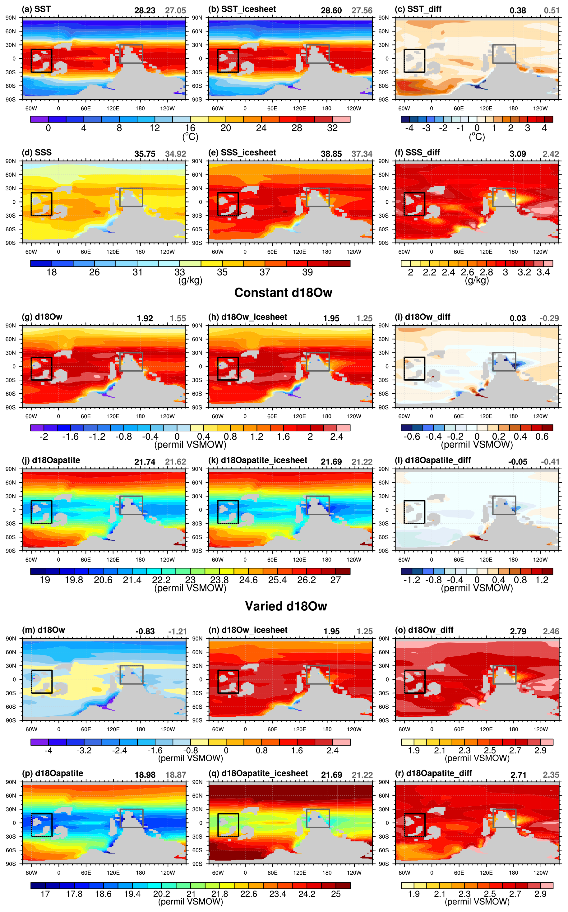
Figure B1 Simulated and calculated effects of land-ice growth on low-latitude oxygen-isotope records. Left, middle, and right columns show the case CTRL, the coupled ice-sheet experiment, and their differences, respectively. Rows 1 and 2 show simulated SST (a–c) and SSS (d–f). In the coupled ice-sheet experiment, SSS has been corrected for the global salinity increase expected from the transfer of seawater to land ice based on salt conservation. Rows 3 and 4 show the calculated surface δ¹⁸O_w (g–i) and δ¹⁸O_apatite (j–l), assuming a fixed background seawater oxygen-isotope composition, δ¹⁸O₀, between the two experiments. Rows 5 and 6 show the same calculations for δ¹⁸O_w (m–o) and δ¹⁸O_apatite (p–r), but allowing δ¹⁸O₀ to vary with land-ice volume. The black and dark-gray boxes denote low-latitude regions corresponding to possible Ordovician oxygen-isotope records from Laurentia, including the Anticosti Island region, and Gondwana, including Australia, respectively. The black and dark-gray numbers in the upper-right corner of each panel indicate the area-weighted mean values within the black and dark-gray boxes, respectively.

Appendix C: supplementary figures

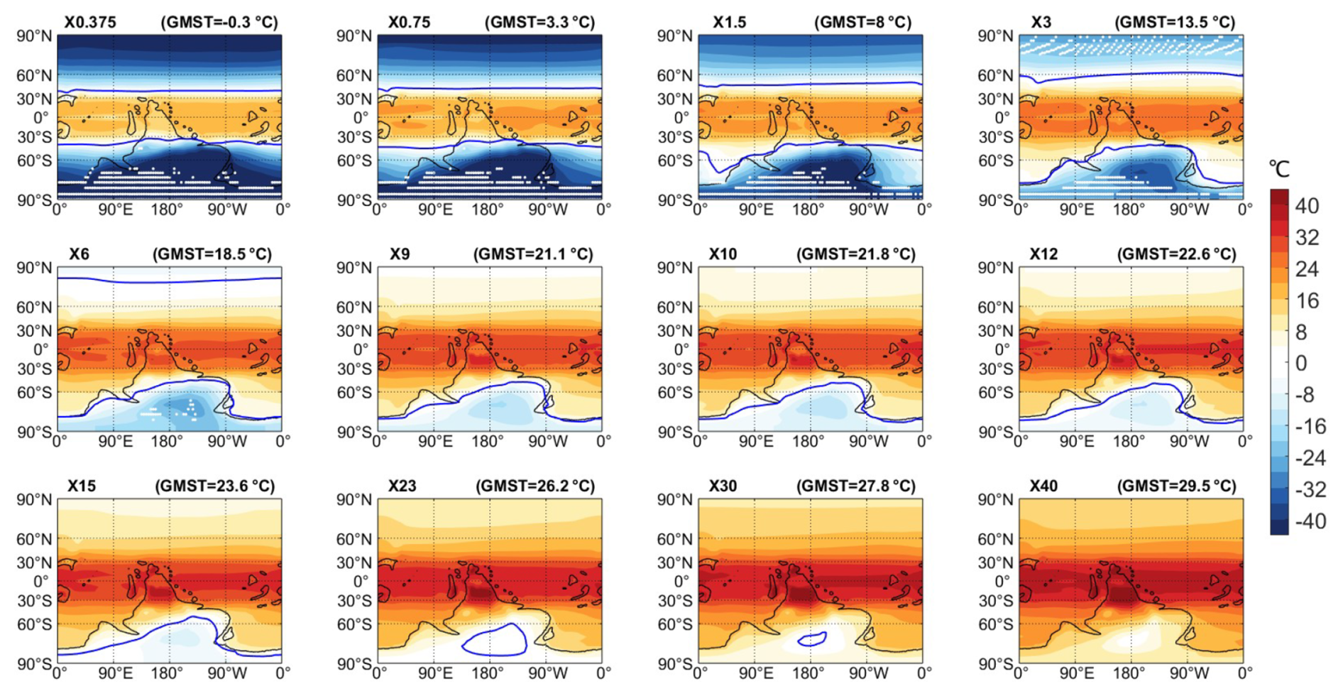
Figure C1 Late Ordovician climate sensitivity to CO₂. Annual mean surface temperature under different PAL CO₂ conditions. White dots represent the extent of the cryosphere: sea ice is defined based on the annual mean sea ice fraction (indicating perennial ice), while land ice is defined as areas where the annual mean water-equivalent snow depth exceeds 1 m, representing potential regions for continental ice development. The results show that, in the uncoupled ice sheet scenario, a CO₂ level of 6 PAL marks the threshold for initiating continental ice formation, whereas only when greenhouse gas concentrations drop sufficiently low (∼ 1 PAL) can land ice marginally extend to around 60° S. The development of sea ice in the SH ocean lags that of land ice. The blue solid lines represent the 0 °C.

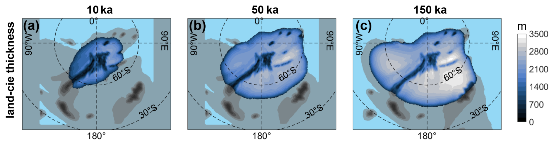
Figure C2 Land-ice thickness in case CP. Three snapshots from the coupled framework simulation at (a) 10 ka, (b) 50 ka, and (c) 150 ka. Latitude is shown at 30° intervals.

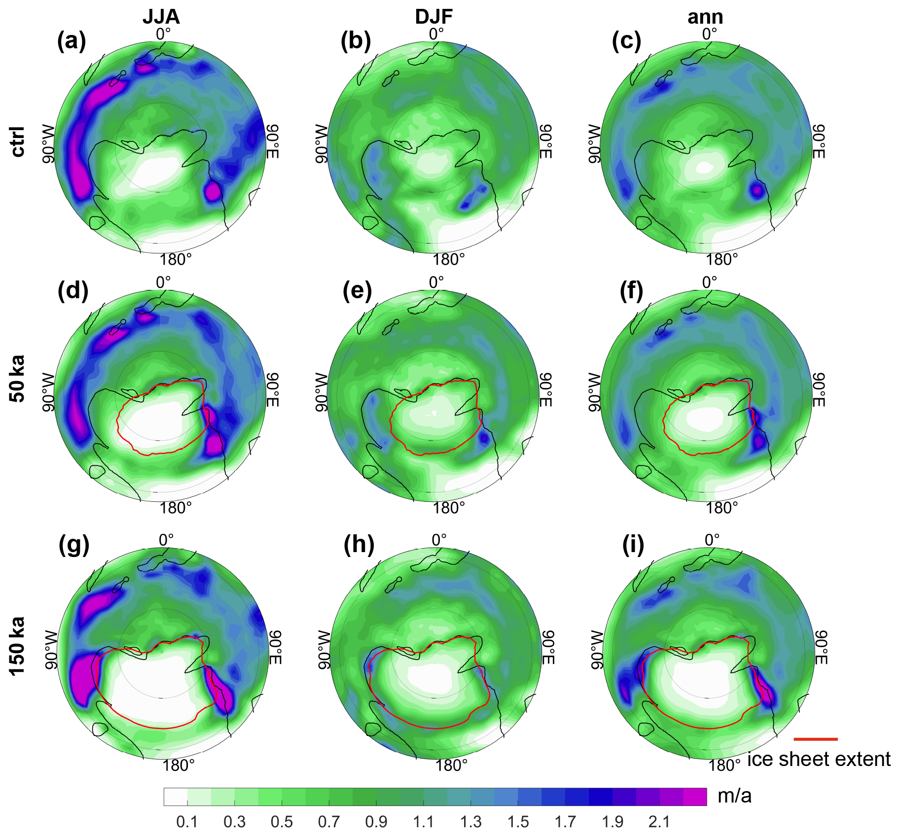
Figure C3 Evolution of precipitation fields. (a–c) Precipitation fields for the case CTRL. Two snapshots for the coupled run: (d–f) 50 ka, (g–i) 150 ka (equilibrium state). From left to right, the three columns represent the austral winter (June, July, and August; JJA); the austral summer (December, January, and February; DJF), and the annual mean, respectively.

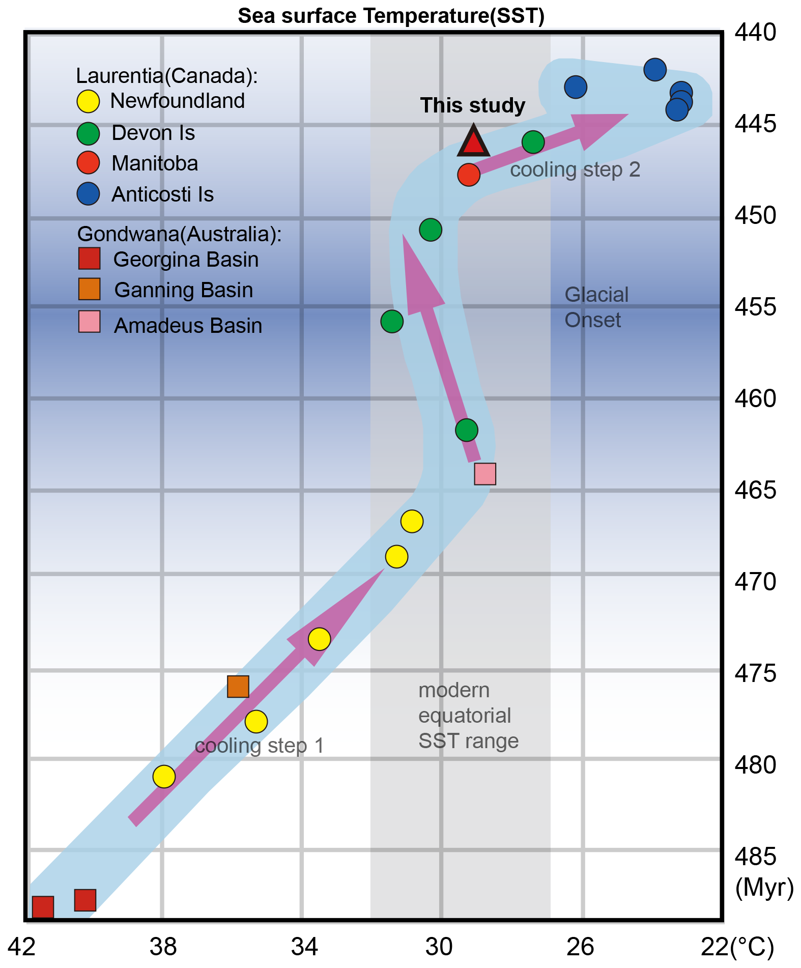
Figure C4 Tropical seawater temperature trend. Generalized tropical seawater temperature trend throughout the Ordovician, derived from conodont oxygen isotope compositions measured in situ. Temperature means are plotted for different analytical sessions. The blue line represents the primary first-order temporal trend of Ordovician sea-surface temperatures. The red triangles represent the tropical sea surface temperatures from this study. Note that these temperatures do not correspond directly in time but have been placed at the Mid-Ordovician based on corresponding temperatures (Redrawn from Trotter et al., 2008).

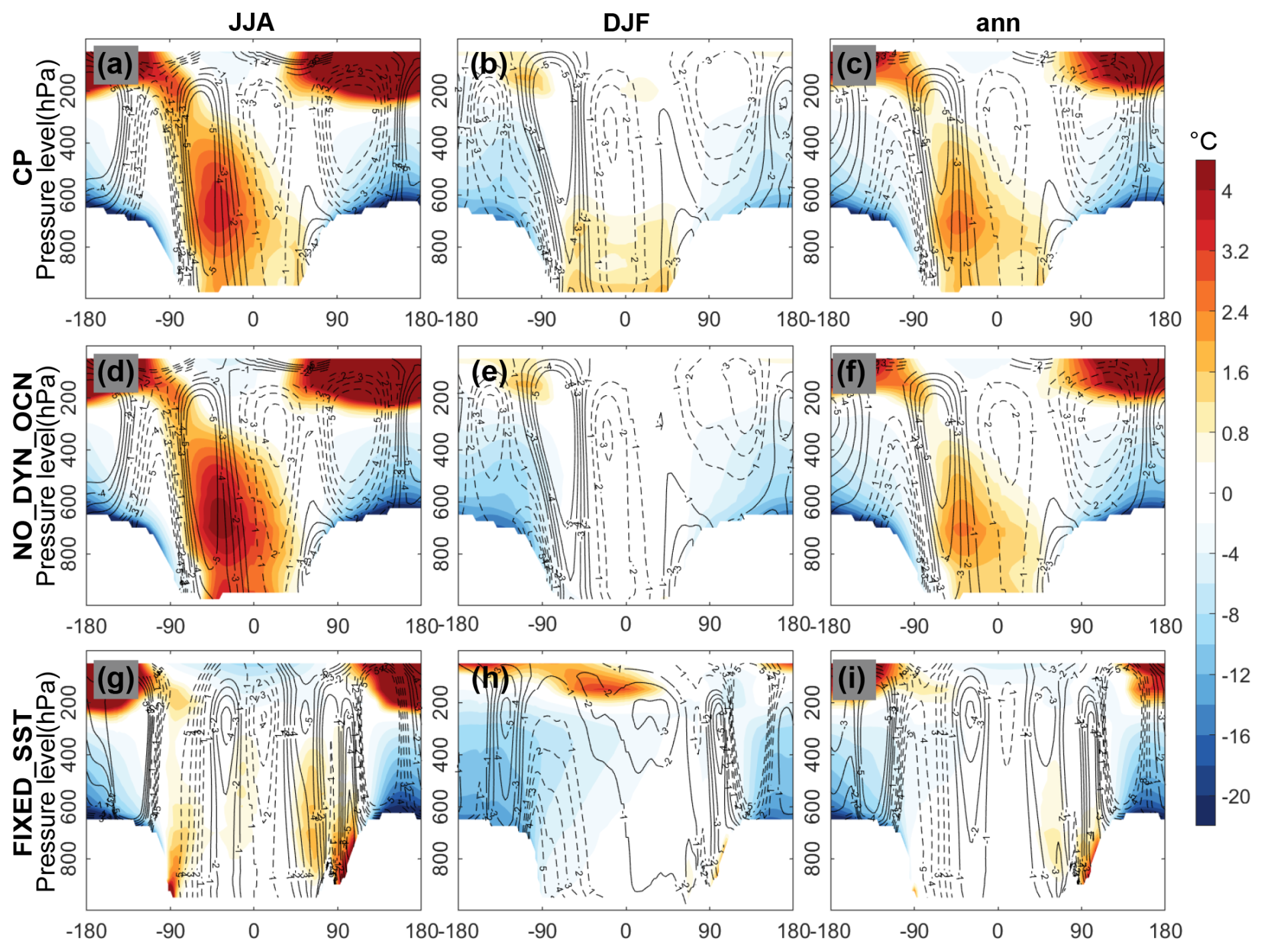
Figure C5 65° S profile, with shaded areas representing temperature and contour lines representing meridional wind. Solid lines indicate northerly winds, and dashed lines indicate southerly winds. Note that the color scale is uneven when showing temperature differences, while the warming section has been artificially amplified. Time average for March, April, May (MAM); austral winter (June, July, and August, JJA); September, October, November (SON); austral summer (December, January, and February, DJF) and annual means.

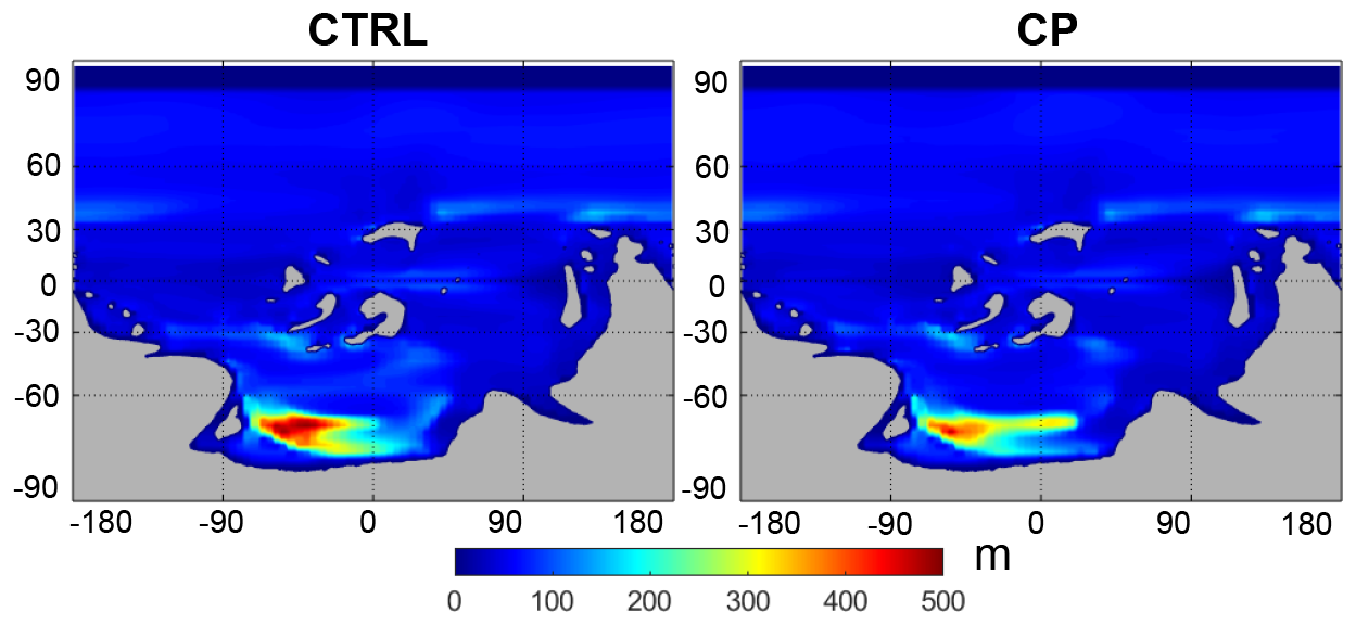
Figure C6 Comparison of mixed-layer depth between the CTRL and CP experiments. Shading indicates mixed-layer depth (m).