The Marine Isotopic Stage 7: a relic of the “41 ka world”? Perspectives from a global-scale sea-surface temperature synthesis

The Marine Isotope Stage 7 (MIS 7, ∼ 245–190 ka) displays an unusual morphology compared to the other interglacials of the late Pleistocene. It comprises two major warm periods (MIS 7e and MIS 7c) each preceded by multi-millennial-scale warming intervals (Termination III (TIII) and TIIIa, respectively) and separated by a brief return to glacial conditions (MIS 7d). When considered as two distinct warm phases, MIS 7 has been compared to the 41 ka obliquity-driven climate cycles of the pre-mid-Pleistocene transition (MPT) world. However, a coherent spatio-temporal picture of MIS 7 surface temperature remains lacking to enable a comprehensive comparison with other interglacials. Here we compiled 132 high-resolution (better than 4 ka) sea surface temperature (SST) records derived from 85 marine sites over the time interval 260–190 ka. In order to provide a spatio-temporal comparison of these records, we (i) align them on a common temporal framework relying on the AICC2023 reference ice core chronology and (ii) recompute SSTs using a homogenized proxy-calibration, both steps applying Bayesian and Monte Carlo approaches to quantify the attached uncertainty. Finally, we produce global and regional stacks of SST anomalies relative to the pre-industrial covering TIII and the following MIS 7.

Our results evidence that global mean surface temperature remains below pre-industrial (PI) values over both MIS 7e (−1.4 ± 0.3 °C) and MIS 7c (−1.0 ± 0.3 °C) periods. The warmest phase across MIS 7 occurs during the MIS 7c substage, although the global surface temperature difference compared to MIS 7e is within uncertainty of the reconstruction (around 0.4 ± 0.4 °C warmer). MIS 7c is a period when atmospheric CO₂ concentrations are 30 ppm lower than during MIS 7e. This result illustrates a transient decoupling between radiative forcing and the global surface temperature response during periods of CO₂ overshoot, after which global temperature re-equilibrate with CO₂ concentrations. In addition, TIII exhibits a greater warming amplitude than TIIIa, both globally and regionally. The spatial and temporal dynamics of the two terminations differ markedly. TIII follows a “classic” sequential deglaciation pattern, with an early warming initiated in the Southern Hemisphere, which then gradually propagates toward the Northern Hemisphere. In contrast, TIIIa displays near-synchronous warming across all latitudes, lacking the interhemispheric pattern typical of classical terminations. This suggests that TIIIa is not a standard glacial termination, but rather a distinct climatic transition likely caused by the most extreme obliquity values of the Pleistocene occurring over this period. We therefore propose that TIIIa is the result of a self-sustained climatic oscillation that temporarily re-synchronised to the 41 ka cycles because of an exceptional orbital context. As a result, MIS 7 represents a hybrid interglacial, embedded within the post-MPT 100 ka framework, yet shaped by obliquity-driven forcing such as during the early Pleistocene.

1 Introduction

Interglacial periods of the Pleistocene are characterized by a wide diversity of external orbital forcing, ice-sheet configurations, atmospheric greenhouse gas concentrations, and global-to-regional climate patterns (Lang and Wolff, 2011; Past Interglacials Working Group of PAGES, 2016; Tzedakis et al., 2009). This diversity offers a unique opportunity to investigate the mechanisms driving the establishment of warm climates under different boundary conditions. Global-scale syntheses of multi-archive-based surface temperature records rely on harmonized paleorecords from different regions across the Earth, which is essential to investigate the spatio-temporal evolution of climate changes. Such approach has been applied to the current interglacial (the Holocene), the last interglacial (Marine Isotope Stage 5e, MIS 5e), MIS 9, and MIS 11, as well as to their respective preceding Termination I (TI), TII, TIV and TV, relying on the abundance of highly resolved paleoclimate records spanning these intervals (Capron et al., 2014; Hoffman et al., 2017; Milker et al., 2013; Osman et al., 2021; Stevenard et al., 2025). Furthermore, they offer key comparative insights into present-day climate dynamics and establish benchmarks for climate model simulations to enable robust data–model comparisons (e.g. Capron et al., 2017; Gao et al., 2025; Hoffman et al., 2017). MIS 5, MIS 11 and MIS 9 stand out as warm interglacials of the last 800 ka and are representative of the late Pleistocene interglacials occurring after the Mid-Pleistocene Transition (MPT, ∼ 1.2–0.7 Ma; Berends et al., 2021a; Past Interglacials Working Group of PAGES, 2016). In contrast, MIS 7 (∼ 245–190 ka) remains relatively understudied, in part due to its weaker climatic optimum compared to other late Pleistocene interglacials, making it less relevant than MIS 5 or MIS 11 to inform on the state of the Earth system components in a warmer-than pre-industrial (PI) context.

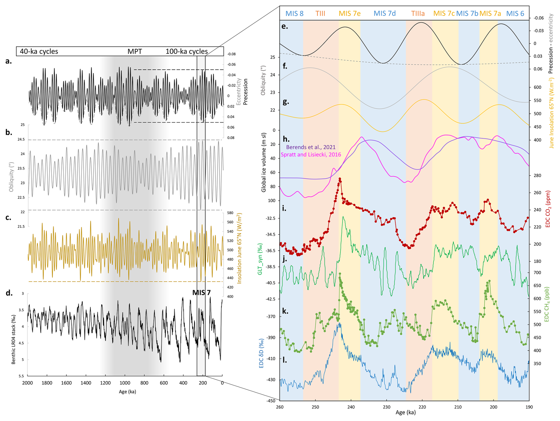
Figure 1 Left: MIS 7 shown within the context of the past 2 million years. From top to bottom: (a) precession (black), eccentricity (grey) (Laskar et al., 2004), (b) obliquity (Laskar et al., 2004), (c) June insolation at 65° N (Laskar et al., 2004), and (d) the benthic LR04 δ¹⁸O stack (Lisiecki and Raymo, 2005). The grey box highlights TIII and MIS7. The shaded area marks the interval of the Mid-Pleistocene Transition. Dashed horizontal lines indicate the maximum and minimum orbital values (precession evaluated over 800–0 ka; obliquity and June 65° N insolation over 2000–0 ka). All of these extrema occur during the MIS 7 interval. Colour coding: black shows the precession extrema over the last 800 ka, grey corresponds to obliquity extrema over the past 2 Ma, and yellow represents the minimum June 65° N insolation over the past 2 Ma. Right: Orbital and climatic datasets spanning 260–190 ka. From top to bottom: (e) eccentricity (dotted) and precession (solid) (Laskar et al., 2004), (f) obliquity (Laskar et al., 2004), (g) June insolation at 65° N (Laskar et al., 2004), (h) global ice-volume estimates expressed as sea-level equivalents from Berends et al. (2021b) (purple) and Spratt and Lisiecki (2016) (pink), (i) atmospheric CO₂ record from the EPICA Dome C ice core (EDC) (Legrain et al., 2024), (j) Greenland synthetic temperature curve GLT_syn (Barker et al., 2011), (k) Atmospheric CH₄ record from EDC (Legrain et al., 2024; Loulergue et al., 2008), and (l) EDC δD record (Jouzel et al., 2007). Ice core records are aligned onto the AICC2023 chronology (Bouchet et al., 2023). The colored shaded areas help to identify the different climatic periods discussed in this study, but do not correspond to a strict definition. We acknowledge that these boundaries are arbitrary, but they are only used here to clarify reference to the climatic intervals throughout the manuscript.

The structure of MIS 7 is well documented in the Antarctic ice core archive, through both local temperature proxies (Landais et al., 2021; Watanabe et al., 2023) and global atmospheric greenhouse gas reconstructions (Legrain et al., 2024; Loulergue et al., 2008; Petit et al., 1999) (Fig. 1i, j). It is also recorded in a variety of marine and continental proxy records (e.g. Desprat et al., 2006; Martrat et al., 2007; Roucoux et al., 2008; Wendt et al., 2021). MIS 7 follows TIII and is composed of several sub-stages, starting with the warm stage MIS 7e, which is marked by an abrupt onset and coincides with an overshoot in atmospheric CO₂ concentrations (Legrain et al., 2024). This phase is followed by a return to glacial conditions during MIS 7d, characterized by low CO₂ concentrations characteristic of a full glacial period (< 200 ppm, Legrain et al., 2024). Subsequently, a major warming event occurs, referred to as TIIIa, around ∼ 218 ka, leading into the warm stage MIS 7c. The amplitude of TIIIa in Antarctic surface temperature and atmospheric CO₂ records is smaller than that of the preceding TIII (Jouzel et al., 2007; Legrain et al., 2024). However, regional climate reconstructions based on pollen and biogenic silica suggest that the climatic response during TIIIa was comparable to, or even exceeded, that of TIII (Prokopenko et al., 2006; Roucoux et al., 2008). Due to its relatively modest CO₂ concentrations, MIS 7c has occasionally been excluded from interglacial lists under stricter CO₂-based definitions (Tzedakis et al., 2009, 2012). However, under sea-level and benthic δ¹⁸O criteria, it is classified as a distinct interglacial (Past Interglacials Working Group of PAGES, 2016). This period concludes with a short and relatively poorly marked stage MIS 7b. Finally, the climate system enters a third warm interval, MIS 7a, before gradually transitioning into the full glacial conditions of MIS 6 around 190 ka. Depending on the resolution and geographical location of the records, MIS 7a and MIS 7c may not be distinguished. Consequently, we considered MIS 7c, MIS 7b and MIS 7a as a single interval referred to as MIS 7c in the discussion section.

Global ice-volume variations during MIS 7 remain poorly constrained (Dutton et al., 2009; Lea et al., 2002; Siddall et al., 2003; Spratt and Lisiecki, 2016). Conceptual models driven solely by orbital forcing struggle to replicate the various data-derived ice volume reconstructions, capturing only part of the complexity of the climatic sequence (Imbrie et al., 2011; Legrain et al., 2023; Parrenin and Paillard, 2012). The relative influence of orbital vs. greenhouse gases forcings has also been investigated using more sophisticated physical models (Choudhury et al., 2020; Colleoni et al., 2014; Ganopolski and Brovkin, 2017).

The complex structure of MIS 7, characterized by a double warm peak, differs from the other recent interglacials (Fig. 1). Because of its relatively cold temperature optimum and its two-peaks morphology, MIS 7 has been compared to the pre-MPT cycles, characterized by a 41 ka periodicity and a relatively low amplitude (Tzedakis et al., 2012; Watanabe et al., 2023). The occurrence of the two-peaks during MIS 7, among of the single-peak interglacials MIS 1, MIS 5, MIS 9 and MIS 11 remains unexplained, although it is suspected to be linked to the exceptional amplitude of orbital variations during this period (Tzedakis et al., 2012, 2017) (Fig. 1a, b, c). Given this pattern of climatic variability, MIS 7 provides an excellent framework for examining how the climate responds at both regional and global scales, as well as how these responses relate to orbital forcing and the carbon cycle. The variety of global and regional climate signals recorded during MIS 7, along with the need to identify their respective drivers, calls for an approach that accounts for the spatial and temporal heterogeneity of the warming, as performed in syntheses for the other interglacials (e.g. Capron et al., 2014; Hoffman et al., 2017; Stevenard et al., 2025). To date, only few syntheses have compiled sea surface temperature (SST) records spanning this period (e.g. Clark et al., 2024; Lang and Wolff, 2011; Shakun et al., 2015; Snyder, 2016). However, these syntheses rely on a limited number of paleoclimatic records and primarily target longer timescales (≥ 800 000 years). Hence, they are largely composed of low-resolution (albeit temporally extensive) records that are aligned to the LR04 benthic δ¹⁸O stack, which was dated through orbital tuning. By focusing on MIS 7 and Termination III, a larger number of higher-resolution records can be aligned within a more robust chronological framework, thereby enabling a more detailed characterization of the spatio-temporal variability in surface temperature during this interval.

In this study, we provide the first SST compilation focused on the MIS 7 and TIII interval in which surface temperature records are aligned on a unified chronological framework. Relying on this synthesis, we (i) assess how the magnitude of warming varied spatially between TIII and TIIIa and between MIS 7e and 7c, (ii) describe the temporal evolution of sea-surface temperatures across major ocean basins, and (iii) place MIS 7 within the broader context of Pleistocene climate cycles.

2 Material and methods

The methods used for the SST synthesis construction and the stacking over TIII and MIS 7 are identical to those employed in Stevenard et al. (2025), which focused on TIV and MIS 9. Below is a summary of the main steps, while a detailed description of the methodology and calibration modelling choices can be found in Stevenard et al. (2025).

2.1 Selection of paleoclimatic data sites

We compiled 132 SST records from 85 marine cores spanning the 260–190 ka interval (Fig. 2). We apply a threshold resolution filter of 4 ka, leading to an average resolution of 1.7 ka for the whole dataset. 106 and 26 of the records represent annual and seasonal temperatures, respectively. Four different SST proxies are included in the synthesis: the alkenone unsaturation index ($U_{\mathrm{37}}^{k^{\prime }}$), the Modern Analog Technique (MAT) relying on faunal microfossil assemblages, the ratio of magnesium to calcium (Mg $/$ Ca) and the oxygen isotope (δ¹⁸O_p) of planktic foraminifera (Fig. 2). Table S1 compiles all details of the selected records.

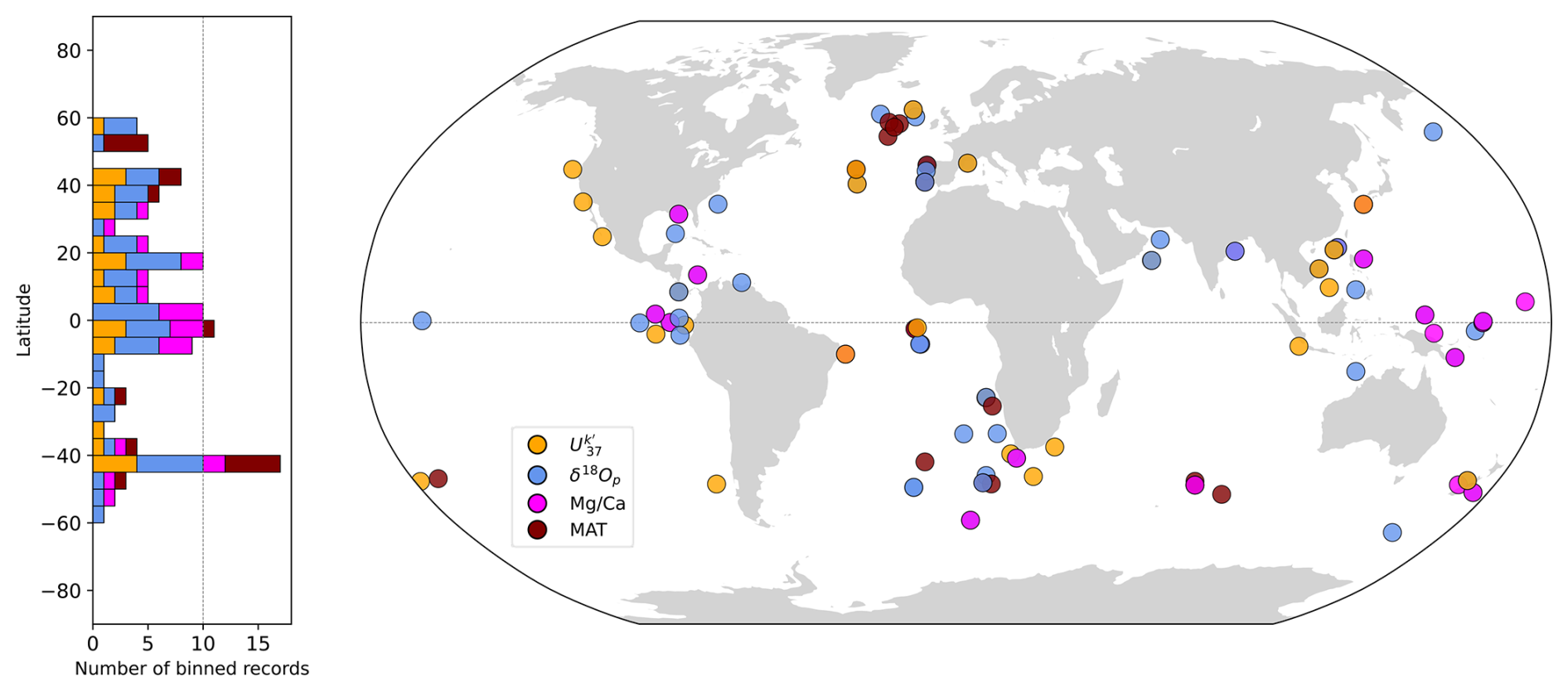
Figure 2 Location and latitudinal distribution of SST records. Left: Distribution of the records per 5° latitude bins. Right: SST reconstructions based on $U_{\mathrm{37}}^{k^{\prime }}$ (orange), δ¹⁸O_p (blue), Mg $/$ Ca (pink) and Modern Analog Technique (MAT) (brown).

2.2 SST calibrations

Following the approach developed in Stevenard et al. (2025), we recalibrate the original SST records applying a Bayesian approach.

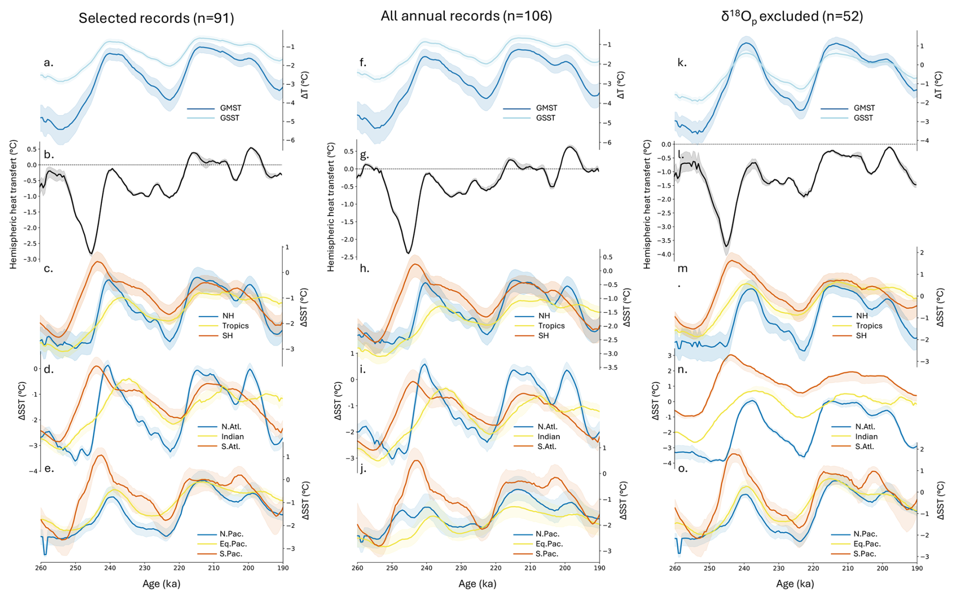
Figure 3 Sensitivity tests on the stacking procedure. (a–e) Stacks built from selected SST records (15 records excluded, chosen version for this study); (f–j) stacks including all annual records. (k–o) Stacks excluding δ¹⁸O_p-based SST records. (a, f, k) Global ΔGSST (light blue) and ΔGMST (dark blue) stacks; (b, g, l) Hemispheric heat transfer (black line), computed as the Northern Hemisphere minus Southern Hemisphere temperature stacks. (c, h, m) hemispheric ΔSST stacks for the Northern Hemisphere (blue), Tropics (yellow), and Southern Hemisphere (red); (d, i, n) Atlantic and Indian Ocean ΔSST stacks for the North (blue), South (red) Atlantic and Indian Ocean (yellow); (e, j, o) Pacific ΔSST stacks for the North (blue), Equatorial (yellow), and South (red) Pacific.

To calibrate the 27 $U_{\mathrm{37}}^{k^{\prime }}$ records, we applied a Bayesian calibration with a prior standard deviation of 5 °C using the BAYSPLINE Matlab package that produced a N×1000 matrix of SST possibilities for each age N (Tierney and Tingley, 2018). The 22 Mg $/$ Ca records are calibrated with a Bayesian calibration using the BAYMAG Matlab package (Tierney et al., 2019), applying a prior standard deviation of 6 °C (Osman et al., 2021). The seawater salinity and pH estimates are defined with a modified function from Gray and Evans (2019) and using the benthic stack LR04 (Lisiecki and Raymo, 2005) as reference for sea-level changes. This calibration produces a N×2000 Mg $/$ Ca matrix of SST possibilities for each age N then randomly subsampled to produce a N×1000 matrix. To calibrate the 55 δ¹⁸O_p records, we used the BAYFOX Matlab package, applying a Bayesian calibration with a prior standard deviation of 10 °C that produced a N×1000 δ¹⁸O_p matrix of SST possibilities for each age N (Malevich et al., 2019). The prior sea water d¹⁸O values were estimated from the Breitkreuz et al. (2018) database and the ice-volume correction use the benthic LR04 stack (Lisiecki and Raymo, 2005) as reference. We decided to include δ¹⁸O_p, although this proxy reflects both temperature and hydrographic changes, notably variations in seawater δ¹⁸O linked to salinity. While we correct δ¹⁸O_p for seawater δ¹⁸O, SST estimates derived from this proxy should still be interpreted with caution. We therefore also provide alternative global and regional stacks excluding these records from the synthesis (Fig. 3). To our knowledge, no Bayesian approach has been developed for MAT calibrations. We propagate the uncertainties of the 28 MAT records applying a Monte-Carlo analysis creating 1000 scenarios for each data point that follows a normal distribution based on the uncertainty σ provided in the original publications. If this error (σ) was not published in the original publications, we estimated it as the standard deviation of the SST record over the period 260–190 ka period. To be consistent with other approaches, the ensemble of MAT records is a N×1000 matrix.

2.3 Anomaly from the pre-industrial period

Following approaches developed in previous interglacial syntheses, the SST records are transferred into anomaly compared to the pre-industrial (PI) (e.g. Capron et al., 2014; Hoffman et al., 2017; Osman et al., 2021; Stevenard et al., 2025). As most of the records have no core-top data indicative of recent SST, PI-SST are derived from the HadISST database (Rayner et al., 2003) over the 1870–1899 interval (Capron et al., 2017; Stevenard et al., 2025). These PI-SST were forward modelled to estimate a proxy-value relative to the PI-SST, and then recalibrate using the Bayesian calibrations described above to propagate the proxy-based SST uncertainties for the PI period (Osman et al., 2021; Stevenard et al., 2025).

2.4 Chronologies

In this study, we harmonize the chronologies of marine sediment records using a three-step approach based on alignment to ice core and speleothems records, and Bayesian modelling (Stevenard et al., 2025). All alignments are performed with the AnalySeries software (Paillard et al., 1996). We apply a strategy similar to previous syntheses by aligning high-latitude basin reference records to surface air temperature reconstructions from Antarctic (δD of EPICA Dome C) and Greenland ice cores (Hoffman et al., 2017; Stevenard et al., 2025; Vázquez Riveiros et al., 2010). At Site U1429 (the reference for Northwest Pacific), we synchronized the planktic δ¹⁸O_notched record of G. ruber, which is the δ¹⁸O signal with eccentricity- and obliquity-band components removed (Clemens et al., 2018) interpreted as a proxy for East Asian monsoon variability, with the δ¹⁸O_calcite stack from the Sanbao Cave (Cheng et al., 2016). The Sanbao δ¹⁸O_calcite series was already been placed on the AICC2023 timescale by linear interpolation between the tie points defined by Bouchet et al. (2023). For Greenland, where direct surface air temperature reconstructions are unavailable beyond 130 ka, we use the synthetic temperature curve GLT_syn (Barker et al., 2011). We do not use directly the CH₄ records as the terrestrial biosphere response to hydroclimatic changes in lower latitudes may affect the CH₄ concentrations and decoupled them from Northern Hemisphere sea surface temperature changes at high latitudes (Kleinen et al., 2023). Despite some millennial-scale discrepancies with CH₄ and Greenland isotope records, GLT_syn provides a practical reference for northern high-latitude temperature and has been widely used to align marine records with ice-core chronologies (e.g., Barker et al., 2015; Hodell et al., 2023). Then, every record in an oceanic basin is aligned to the reference record through benthic foraminifera δ¹⁸O record. In case of absence or low-resolution of a benthic δ¹⁸O record, the SST is directly aligned on the ice core record for high-latitude sites (> 40° N or S), or to the closest already-aligned record for low-latitude sites (< 40° N or S). Then, the age and depth uncertainties associated with the alignment are merged into a single age uncertainty through a Bayesian approach (10⁵ iterations) using the “Undatable” software (Lougheed and Obrochta, 2019) with a xfactor of 0.1 and no bootstrap. The absolute age uncertainty is estimated by calculating the quadratic sum of all uncertainties (i.e. alignment, basin reference, and ice-core). To build the final chronology of each marine sediment core, we run a final Bayesian age-depth model with the absolute uncertainty, 10⁵ iterations, a xfactor of 0.1 and 15 % of bootstrap through each iteration (Stevenard et al., 2025). Finally, each original SST record corresponds to an ensemble of 1000 probable ages (N×1000 matrix) directly or indirectly aligned to the AICC2023 ice-core chronology (Bouchet et al., 2023).

2.5 Global and regional stack reconstructions

To estimate global SST anomalies during MIS 7, we used the “sststack” Python package (Stevenard et al., 2025) built to facilitate the stacking of ensemble-based SST. It includes the Monte Carlo approach detailed in Stevenard et al. (2025). The ensemble of both age and SST is redrawn to ensure that Nth age-SST pairs are different for each iteration. To reduce spatial bias, we apply a three-step averaging procedure within each Monte Carlo iteration and for each 500-year time bin: (1) we first average all SST ensemble values available at each site, regardless the proxy type; (2) we then average these site means within a randomly defined spatial grid (grid size randomly selected between 2 and 5°); and (3) we finally average the gridded values within randomly defined latitudinal bands (band width randomly selected between 2.5 and 10°). Global and regional SST stacks at hemispheric (North, Tropics, South) and ocean-basin scales (North Atlantic, North Pacific, Equatorial Pacific, South Atlantic, Indian Ocean and South Pacific) were calculated at each iteration. All stacks were defined as the weighted mean of all latitudinal band averages, with each band weighted according to its proportional surface area (i.e., cosine of latitude). The global mean surface air temperature (ΔGMST) is defined as the global SST anomaly (ΔGSST) using a random factor (1.5–2.3) derived from climate model comparisons (Osman et al., 2021; Snyder, 2016; Stevenard et al., 2025). As no sites are located north or south of 60°, polar amplification is not directly represented in the ΔGSST stacks, which therefore reflect extrapolar mean conditions, whereas it is only accounted for in the derived ΔGMST reconstruction. This Monte Carlo process is repeated 10 000 times to ensure the propagation of all uncertainties.

3 Results

3.1 Sensitivity tests of global and regional stacks

Based on the specific description of individual records (Sect. S1 in the Supplement, Figs. S1, S2 ,S3), we identified discrepancies among SST reconstructions from the same sites (i.e., using different proxies) and, in some cases, within the general trends of a given region. Most inconsistencies are associated with δ¹⁸O_p- and, to a lesser extent, Mg $/$ Ca-derived SSTs. This observation has also been made in the MIS 9 synthesis from .Stevenard et al. (2025) and likely reflects a lack of environmental constraints used for calibrations. To assess the influence of these records on the stacking procedure, we performed three sensitivity tests: (1) including all annual SST records (n = 106); (2) excluding all δ¹⁸O_p-based SST reconstructions (n = 56), which may yield lower temperature estimates or distinct variability patterns; and (3) retaining only records showing consistent amplitude and/or variability within the same region, resulting in the exclusion of 15 records (n = 91), mostly derived from δ¹⁸O_p and Mg $/$ Ca proxies (Fig. 3). The selection in this third test was based on visual assessment, and the list of excluded record is given in the Supplement (Sect. S1.8).

Overall, the resulting stacks exhibit highly consistent variability across the different tests, independent of the method applied. At both global and hemispheric scales, the amplitude and timing of the main climatic features (e.g., glacial inception, glacial termination and interglacial optimum) remain virtually unchanged. As in the MIS 9 synthesis (Stevenard et al., 2025), the absence of δ¹⁸O_p shifted South Atlantic and Indian Ocean stacks towards warmer value (+1 to 3 °C). The tests including all records (1) and the one only excluding 15 selected records (3) are very similar, with temperature slightly colder for the “all records” stacks (−0.3 °C in average for GMST and GSST stacks). The main regional difference occurs in the Equatorial and Northern Pacific with a more pronounced (+1 °C) and better-defined MIS 7e in the “selected” record stacks. This result confirms the potential bias of proxies influenced by other parameters than sea surface temperature (e.g. water salinity) in region where water properties can change drastically due to regional climate (e.g. monsoon events).

Excluding all δ¹⁸O_p-based SST records (2) nearly halves the number of available records and reduces the spatial coverage of the synthesis prior to stacking, particularly in the South Atlantic sector of the Southern Hemisphere. The “selected” stack (3) represents a compromise approach. Records were excluded only when they displayed trends markedly inconsistent with regional patterns, while most of the available data were retained. The similarity between the “all records” (1) and “selected” stacks indicates that the main large-scale features, structure, and timing of MIS 7 are robust to the choice of compilation. We therefore use the “selected” stack as our primary reference for description and interpretation, while making all three stacking approaches (“all”, “selected”, and δ¹⁸O_p-excluded) available to allow explicit assessment of the sensitivity of the results to proxy selection.

3.2 Basin scale

The regional ΔSST stacks (Fig. 4e) of the different oceanic basins show marked differences in the timing and magnitude of MIS 7 at regional scale: their structure can vary from a structure associated to three temperature peaks clearly identified as the warm substages MIS 7e, 7c and 7a (e.g. North Atlantic) to a signal with low-amplitude (e.g. Equatorial Pacific).

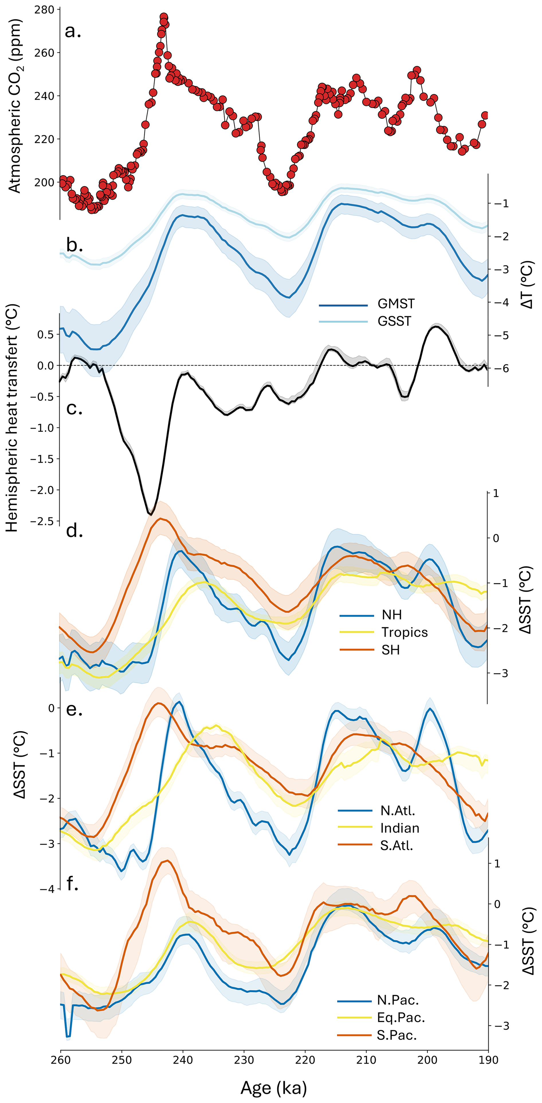
Figure 4 Global and regional records over MIS 7 and Termination III. From top to bottom: (a) Atmospheric CO₂ concentrations (red dots) measured in the EDC ice core (Legrain et al., 2024). (b) ΔGMST (dark blue) and ΔGSST (light blue). (c) Hemispheric heat transfer (black line), computed as the Northern Hemisphere minus Southern Hemisphere temperature stacks. (d) Northern Hemisphere (blue), tropics (yellow) and southern Hemisphere (red) temperature stacks. (e) Basin temperature stacks: North Atlantic (blue), Indian Ocean (yellow), South Atlantic (red). (f) Basin temperature stacks: North Pacific (blue), Equatorial Pacific (yellow), South Pacific (red). All stacks records have been realized with the annual records of the synthesis, at the exception of 15 excluded records (see methods). Colored envelopes are 1σ interval of the corresponding stacks.

During TIII and the following MIS 7e, all basins show a marked warming trend from preceding glacial conditions, though the amplitude and timing of the peak vary. The North Atlantic exhibits the strongest and most abrupt SST rise, reaching PI values, with a TIII amplitude of +3.8 ± 0.2 °C (1σ, here and after) (Figs. 4e and 5) and displays a sharp peak centered around 240 ka. In the South Atlantic and South Pacific, MIS 7e is also well-expressed, but the TIII occurs earlier than in the rest of the basins, around 254 ka, and is slightly lower in amplitude (+3.0 ± 0.3 and +3.7 ± 0.6 °C) compared to North Atlantic. The Indian Ocean also registers a major warming (+2.8 ± 0.1 °C) but with a significant delay, with MIS 7e peak registered around 236 ka. In contrast, the Equatorial and North Pacific basins reveal a less intense warming (+1.8 ± 0.2 and +1.8 ± 0.5 °C, respectively), with MIS 7e expressed as a colder broad plateau (Fig. 4f).

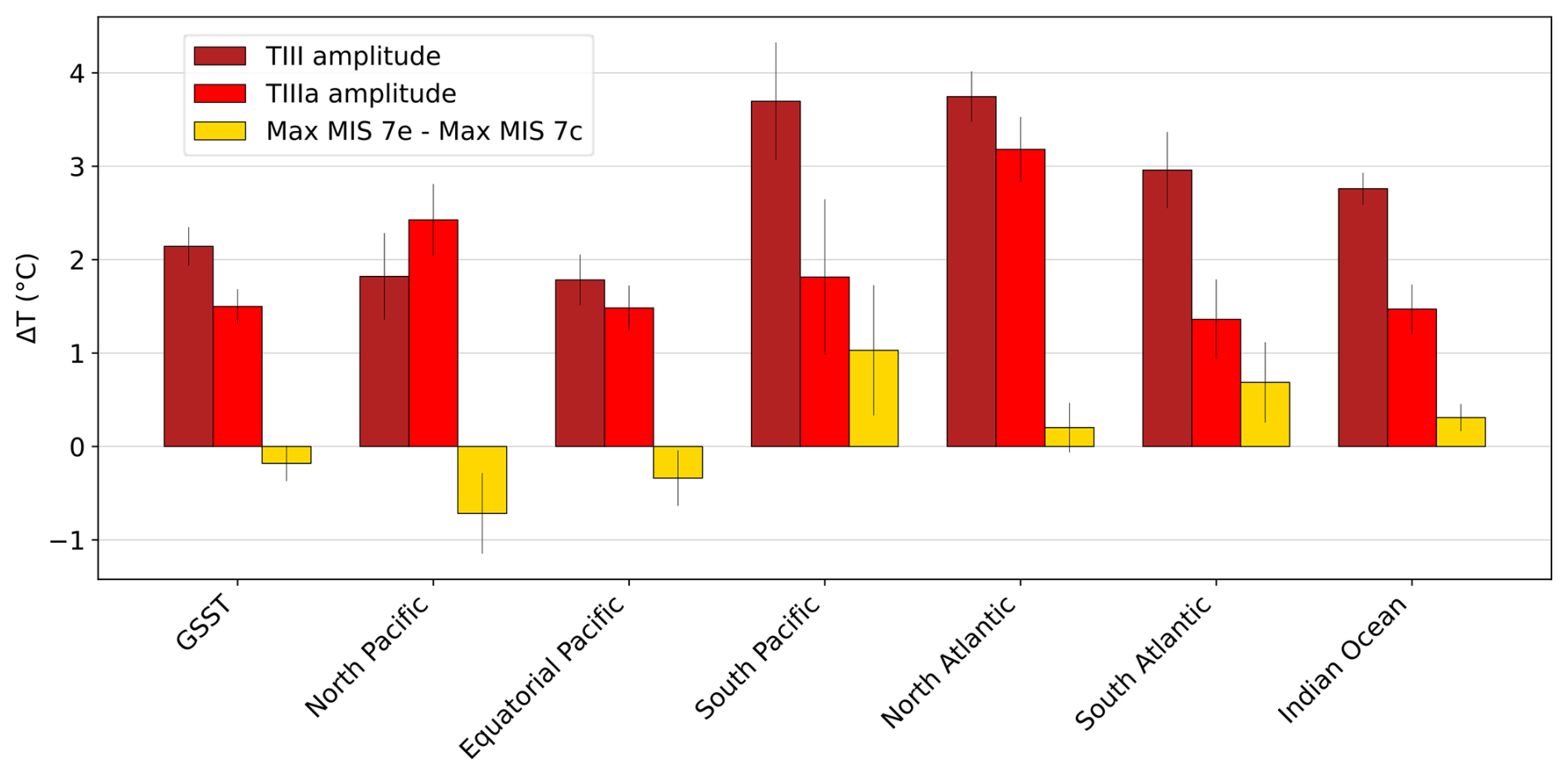
Figure 5 Termination amplitude and warm phases intensity. Amplitude of the temperature change over TIII (dark red) and TIIIa (red) for the GSST stack and regional basin stacks. Difference of interstadials intensity (yellow). Errors bars correspond to 1σ uncertainty.

The MIS 7d cold period is expressed as a distinct cooling in the North Atlantic and South Pacific, with SSTs dropping by 3 °C, marking the two most abrupt stadial onsets in the regional stacks. This cooling is also evident in the South Atlantic, North Pacific and Indian Ocean but occurs more gradually and with reduced amplitude (∼ 2 °C). In the Equatorial Pacific, MIS 7d appears as a subtle inflection of 1 °C (Fig. 4e, f).

The MIS7d is then interrupted by the TIIIa. In general, TIIIa is characterized by a less pronounced warming than TIII, except in the North Pacific, where the temperature rise during TIIIa exceeds that of TIII by 0.2 ± 0.3 °C. During TIIIa, the North Atlantic and the North Pacific exhibits the stronger SST rise, starting at 222ka (+3.1 ± 0.3 and +2.3 ± 0.3 °C respectively) and culminating at around 214 ka. In the four other basins, the warming is of lower amplitude (ranging from +1.3 ± 0.4 °C in South Atlantic to +1.8 ± 0.8 °C in South Pacific) (Fig. 4f).

The following climate optimum corresponds to the MIS 7c. In the North Atlantic, MIS 7c is comparable in magnitude to MIS 7e (Δ7e–c = +0.2 ± 0.3 °C), though more prolonged (Fig. 5). In the North Pacific (−0.7 ± 0.5 °C) and in the Equatorial pacific (−0.3 ± 0.3 °C), MIS 7c is the most prominent substage during MIS 7. In the South Atlantic, South Pacific, and Indian Ocean, MIS 7c peak is colder than MIS 7e (0.7 ± 0.4, 1.0 ± 0.6 and 0.3 ± 0.1 °C respectively).

During MIS 7b, the oceanic basins registered varying degrees of cooling. The North Atlantic and North Pacific shows a clear and rapid SST decline with an identifiable minimum (−1.4 and −1 °C, respectively), while South Pacific exhibit a smoother, more gradual decrease (Fig. 4e, f). The Indian Ocean shows only a weak inflection, and MIS 7b is almost absent in the South Atlantic (Fig. 4e). The Equatorial Pacific maintained an almost flat profile until 190 ka.

MIS 7a is the least consistently expressed of the three warm periods. The North Atlantic, North Pacific and South Pacific exhibit a small but coherent SST rebound following MIS 7b (+1.4, +0.3 and +0.4 °C respectively) though its amplitude is much lower than during TIII and TIIIa. In the Indian Ocean, South Atlantic, and Equatorial Pacific, the signal is barely distinguishable (Fig. 4e).

3.3 Hemispheric scale

Here we present the results from the extra-tropical Northern Hemisphere stack (North of 23° N, referred to as Northern Hemisphere stack after), the extra-tropical Southern Hemisphere stack (South of 23° S, referred to as Southern Hemisphere stack after) and the Tropics stack (between 23° N and 23° S).

The amplitude of TIII is larger in the Southern Hemisphere (3.0 °C) than in the Northern Hemisphere (+2.4 °C) and the Tropics (+2.1 °C), and the only MIS 7 SST values exceeding PI are in the Southern Hemisphere during MIS 7e (+0.5 ± 0.4 °C) (Figs. 4e, 5).

The hemispheric and tropical SST stacks reveal a clear phasing pattern during Termination III and MIS 7e (Fig. 4d). Deglacial warming begins in the Southern Hemisphere around 254 ka and subsequently propagates to the tropical region (warming starting at ∼ 251 ka), with the Northern Hemisphere starting to warm last (∼ 246 ka). The MIS 7e optimum is reached first in the Southern Hemisphere (∼ 244 ka), then in the Northern Hemisphere (∼ 240 ka) and finally in the Tropics (∼ 236 ka). In contrast, no such temporal offset is observed during Termination IIIa, as all regions appear to both initiate warming and reach the optimum synchronously (at ∼ 222.5 and ∼ 214 ka respectively). This phasing difference between TIII and TIIIa is illustrated with the Interhemispheric heat transfer reconstruction, computed as the Northern Hemisphere stack – Southern Hemisphere stack (Fig. 4c). It appears clearly that only the period of TIII registered the large interhemispheric temperature difference (up to 3 °C) characteristic from Terminations, consequent to the delayed warming of Northern Hemisphere associated with a weak AMOC during TIII.

The MIS 7d cold period is very pronounced in both hemispheres, with SSTs dropping by 2 °C (SH) and 2.5 °C (NH), compared to the tropics, while average SSTs decrease by 0.9 °C. MIS 7c evidences similar temperature between Northern and Southern Hemisphere, with MIS 7c slightly warmer than MIS 7e in the Northern Hemisphere (−0.1 ± 0.4 °C) and Tropics region (−0.3 ± 0.1 °C), whereas MIS 7c is colder in the Southern Hemisphere (+0.8 ± 0.5 °C) (Fig. 4d).

Regarding the final stages of MIS 7, only the Northern Hemisphere exhibits a well-defined tripartite interglacial structure (MIS 7e, 7c, 7a), while MIS 7a remains indistinct in both the tropical and Southern Hemisphere stacks.

3.4 Global scale

The ΔGSST and ΔGMST stacks are characterized by a clear two-peak morphology, with prominent interglacials during MIS 7e and MIS 7c. A third warm period, MIS 7a, is also present but expressed with less intensity (Fig. 4b).

TIII has an amplitude of 2.2 ± 0.2 °C in the ΔGSST stack and of 4.1 ± 0.5 °C in the ΔGMST stack, starting at 253.5 ± 0.5 ka. Optimum temperatures during MIS 7e are reached at 240.0 ± 0.5 ka and remain below PI values (−0.7 ± 0.2 and −1.4 ± 0.3 °C). MIS 7d is characterized by a temperature drop of 1.3 and 2.5 °C in the ΔGSST and ΔGMST stacks. MIS 7c appears comparable to, or slightly warmer than MIS 7e (about 0.4 ± 0.4 °C warmer), but remains significantly below pre-industrial levels, with peak anomalies compared to PI of −0.5 ± 0.1 °C (ΔGSST) and −1.0 ± 0.3 °C (ΔGMST) during the climate optimum at 214.0 ± 0.5 ka. Reversely, the amplitude of TIIIa, preceding MIS 7c, is reduced compared to TIII, with ΔT differences between the TIIIa and TIII of −0.7 ± 0.4 °C (ΔGSST) and −1.3 ± 1.1 °C (ΔGMST), respectively (Fig. 5). It illustrates a much warmer MIS 7d compared to MIS 8 (by 1.5 ± 1.0 and +0.8 ± 0.3 °C in ΔGMST and ΔGSST, respectively). MIS 7a is characterized by a temporary warm rebound of less than 0.2 °C in ΔGMST and ΔGSST stacks. At 199.5 ± 0.5 ka, GMST and GSST stacks initiate a cooling leading to MIS 6.

The comparison of MIS 7e and MIS 7c with atmospheric CO₂ concentrations (Fig. 4a) reveals contrasting signals between atmospheric radiative forcing and surface temperature response. In the GMST and GSST stacks, MIS 7c is of similar intensity or slightly warmer than MIS 7e (with 0.4 ± 0.4 and 0.2 ± 0.2 °C ΔGMST and ΔGSST positive anomaly compared to MIS7e). In contrast, the atmospheric CO₂ record shows a higher maximum concentration during MIS 7e (275 ppm) than during MIS 7c (245 ppm).

4 Discussion

4.1 Limitations and contextualization of the synthesis

4.1.1 Limitations of the study

This synthesis was constructed using the same approach and methodology as the MIS 9 surface temperature synthesis by Stevenard et al. (2025). As a result, all approach and methodology-related limitations are similar, and are summarized in the points below:

• Significant discrepancies observed between records from the same site but reconstructed using different proxies represent a major limitation in the interpretation of our SST synthesis during MIS 7. These differences, sometimes substantial, affect both the temporal structure of the variations and the absolute temperature values. These observations can arise (i) from the proxy itself which can integrate other parameters than surface temperature variations (ii) not be representative of the same water depth or (iii) from the Bayesian methodology applied to reconstructed temperature from these proxies. While this limitation is important, it is partially mitigated by the use of intra-basin regional stacks, which help minimizing interpretations based on a single core while providing an analysis of regional trends.

• The use of PI SST reference from the HadISST database (Rayner et al., 2003) can be questioned. Although well-constrained for the PI period, recent comparisons by Gao et al. (2025) show that model-data differences in the Southern high latitudes can reach ±5 °C. This uncertainty may bias the absolute anomaly values reported here. However, all other interpretations than comparison with PI is not affected by this bias.

• This study uses Bayesian methods and Monte Carlo processes to account for uncertainties and produce continuous SST reconstructions. However, uneven spatial coverage, particularly in the Pacific, Indian Ocean, Nordic Seas, and Western Atlantic, may distort latitudinal trends. While this limitation is inherent to all stacking procedures (e.g., Clark et al., 2024; Shakun et al., 2015; Tierney et al., 2020), the stacking process developed in this study aimed to minimize this limitation (Stevenard et al., 2025).

• Differences in the timing of temperature changes across regions, especially during deglaciations and the interglacial peaks, lead to a smoothed global response. Thus, interpreting temperature changes across TIII and MIS 7 requires considering regional, hemispheric, and global GMST stacks together.

4.1.2 Comparison with the synthesis from Clark et al. (2024)

This synthesis of surface temperatures is the first to focus specifically on TIII and MIS 7. While previous global syntheses have examined temperature variations for MIS 7 across much longer timescales, the added value of this study is twofold: (i) it focuses on high-resolution (< 4000 years) data specifically for the MIS 7 period, whereas others rely on averaged resolutions over million-year timescales; and (ii) it aligns this period (260–190 ka) with a chronology not primarily based on orbital targeting (the AICC2023 ice core chronology). This is unlike previous syntheses, which are aligned on the LR04 benthic δ¹⁸O stack dated by fitting an ice volume model to 21 June insolation curve at 65° N, making it highly dependent on orbital forcing and with large absolute uncertainty (±4 ka).

To date, the most comprehensive and up-to-date global synthesis is the one recently published by Clark et al. (2024). Their “high-resolution” synthesis compiled 47 sea surface temperature records of resolution better than 20 ka encompassing the 260–190 ka interval. However, the average resolution of these records is 3.9 ka, close to our resolution threshold (4 ka) and more than double the mean resolution of this study (1.7 ka).

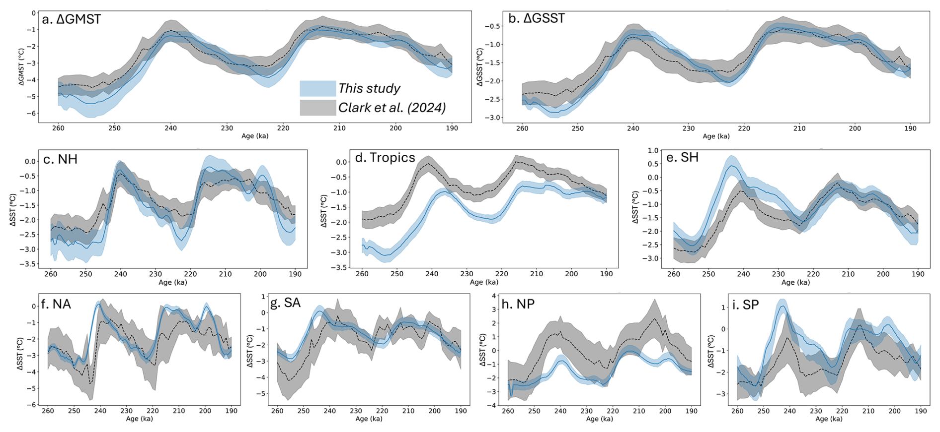
Figure 6 Comparison of our global- and regional-scale temperature reconstructions with those from Clark et al. (2024). All panels: Surface temperature from this study (blue) vs results from Clark et al. (2024) synthesis (black). Black and blue envelopes are σ interval of the corresponding stacks. GMST: Global Mean Surface Temperature. GSST: Global Sea Surface Temperature. NH: Northern Hemisphere. SH: Southern Hemisphere. NA: North Atlantic. SA: South Atlantic. NP: North Pacific. SP: South Pacific. Comparison is not performed for Indian Ocean and Equatorial Pacific stacks as corresponding stacks have not been produced in Clark et al. (2024).

The ΔGSST and ΔGMST derived from the two syntheses exhibit comparable amplitudes, with discrepancies remaining below 1 °C throughout the entire TIII and MIS 7 interval (Fig. 6). The offset between the two ΔGMST is 0.26 ± 0.5 °C in average, with the Clark et al. (2024) synthesis slightly warmer. Nevertheless, pronounced hemispheric differences are revealed with the comparison. During MIS 7e, Southern Hemisphere temperatures are lower in the Clark et al. (2024) synthesis by 1.1 °C and during MIS 7c, Northern Hemisphere is cooler in the Clark et al. (2024) synthesis by 0.7 °C. In terms of timing, the Southern Hemisphere maximum temperature also occurs 3000 years later in the Clark et al. (2024) synthesis compared to this study. Finally, in the tropics, MIS 7e optimum is recorded 3500 years earlier in Clark et al. (2024), and the two syntheses display an average temperature offset of 1 °C over the whole MIS 7 (Fig. 6). At the basin scale, North Atlantic temperatures are colder, whereas North Pacific temperatures are warmer in the synthesis of Clark et al. (2024). The structure of Southern Pacific temperature also diverges between the two reconstructions, with substage MIS 7a absent from Clark et al. (2024) synthesis (Fig. 6).

These findings indicate that the apparent agreement at the global scale primarily reflects compensating regional biases rather than genuine similarity in spatial-scale patterns. This highlights the critical need for high-resolution, temporally constrained syntheses to characterize and discuss the spatio-temporal evolution of surface temperature over a specific interglacial.

4.2 Decoupling of ΔGMST vs. atmospheric CO₂ concentrations over MIS 7e

Past atmospheric reconstructions evidence that maximum atmospheric CO₂ and CH₄ concentrations were significantly higher during MIS 7e than during MIS 7c, with estimated differences of ΔCO₂ = +30 ppm and ΔCH₄ = +100 ppb (Legrain et al., 2024; Loulergue et al., 2008) (Fig. 1i, j). In parallel, Antarctic surface temperatures, reconstructed from water isotopes in ice cores, identify MIS 7e as the warmest phase of the MIS 7 sequence in the high southern latitudes (Fig. 1k). This regional temperature pattern aligns with our Southern Hemisphere SST stacks from the South Atlantic and South Pacific, which both register temperature maxima during MIS 7e. However, these greenhouse gas variations and Antarctic surface temperature reconstructions contrast with the global surface temperature signal. In our ΔGMST reconstruction, MIS 7c appears comparable to, or slightly warmer with global mean surface temperatures 0.4 ± 0.4 °C warmer than during MIS 7e. This result is consistent with the SST synthesis of Clark et al. (2024), which also identifies MIS 7c as slightly warmer than MIS 7e while relying on fewer and less resolved records (Fig. 6). Furthermore, sea-level reconstructions suggest higher stands during MIS 7c than during MIS 7e (Berends et al., 2021b; Spratt and Lisiecki, 2016) (Fig. 1h), reinforcing the interpretation that MIS 7c was not only warmer globally but also associated with a reduced global ice volume. However, this higher peak may also reflect the fact that MIS 7c followed a higher glacial sea-level baseline than MIS 7e (Fig. 1h).

From a radiative forcing perspective, the greenhouse gas difference between MIS 7e (∼ 275 ppm CO₂, ∼ 700 ppb CH₄) and MIS 7c (∼ 245 ppm CO₂, ∼ 600 ppb CH₄) corresponds to an estimated radiative forcing of ∼ 1 W m⁻², which would produce a global temperature change of ∼ 0.8 °C (Hansen et al., 2011; Past Interglacials Working Group of PAGES, 2016). Given that MIS 7e was cooler than MIS 7c by 0.4 °C despite higher GHG concentrations, this implies an anomalous offset of ∼ 1.2 °C between the two periods, suggesting a decoupling between radiative forcing and global temperature response over at least one of them. However, it is important to note that the high CO₂ concentrations observed during MIS 7e are confined to its very beginning (approximately 2 kyr), forming a brief overshoot. After this overshoot, CO₂ concentrations no longer exceed those recorded during MIS 7c (Legrain et al., 2024).

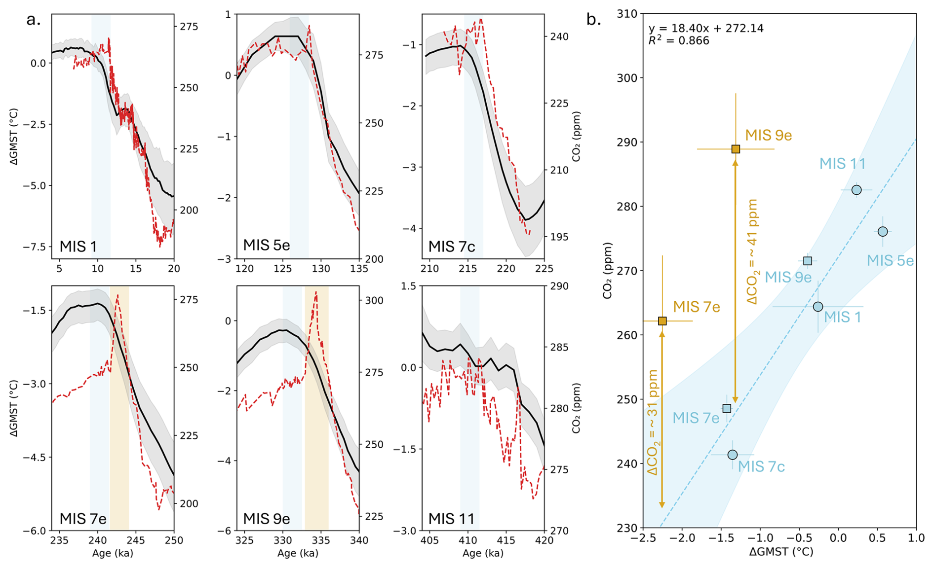
Figure 7 Relationship between GMST and atmospheric CO₂ across the interglacials of the past 450 ka. (a) Global mean surface temperature (GMST; black line with 1σ grey envelope) and atmospheric CO₂ concentrations (red dashed line) for MIS 1 (Bereiter et al., 2015; Osman et al., 2021), MIS 5e (Bereiter et al., 2015; Clark et al., 2024), MIS 7c and MIS 7e (this study; Legrain et al., 2024), MIS 9e (Nehrbass-Ahles et al., 2020; Stevenard et al., 2025), and MIS 11 (Clark et al., 2024; Nehrbass-Ahles et al., 2020). The timescale used for atmospheric CO₂ records is the AICC2023 chronology (Bouchet et al., 2023). Shaded vertical bands indicate the time windows used to compute the window-averaged values shown in panel (b). For MIS 1, MIS 5e, MIS 7c and MIS 11, light blue bands correspond to the 3 kyr time windows following CO₂ concentrations peak. For MIS 9e and MIS 7e, blue/yellow bands denote alternative 3 kyr windows including/excluding the CO₂ overshoot. (b) Dots and square represent window-averaged values derived from the intervals shown in panel (a), with horizontal and vertical error bars indicating the standard deviation of GMST and atmospheric CO₂ concentrations within each window. The dashed line shows the best-fit linear regression, with blue shading indicating the 95 % confidence interval of the predicted mean response. Light blue squares and dots represent interglacials values included in the regression. Yellow squares correspond to values calculated including the CO₂ overshoot for MIS 7e and MIS 9e and are excluded from the regression.

High-resolution records of CO₂ concentrations and GMST estimates are now available over MIS 1 (Bauska et al., 2021; Osman et al., 2021), MIS 5 (Hoffman et al., 2017; Landais et al., 2013), MIS 7 (Legrain et al., 2024; this study), MIS 9 and MIS 11 (Clark et al., 2024; Nehrbass-Ahles et al., 2020; Stevenard et al., 2025). When comparing the average maximum CO₂ concentrations period (3 kyr window following the maximum CO₂ value) with GMST over the same period, it reveals that for MIS 7c, the atmospheric CO₂ concentrations are within the range of expected values considering the GMST over this period and the CO₂ – GMST relationship of the past interglacials (Fig. 7). However, both MIS 7e and MIS 9 evidence anomalously high CO₂ concentrations of 31 ± 14 and 41 ± 13 ppm (1σ), respectively, compared to the expected CO₂ concentrations value based on their GMST (Fig. 7b). These two interglacials are characterized by the most pronounced overshoots of atmospheric CO₂ concentration of the past 500 ka, which consist in an abrupt increase followed by a similarly abrupt decrease of atmospheric CO₂ concentrations at the end of a Termination (Bereiter et al., 2015; Legrain et al., 2024; Nehrbass-Ahles et al., 2020). Over MIS 7e, atmospheric CO₂ concentrations increase and drop by 30 ppm in 2000 years, while during MIS 9 concentrations fluctuate by 35 ppm in 4000 years. In contrast, when considering a 3 kyr window immediately following the CO₂ overshoot, once CO₂ levels have stabilized at typical interglacial equilibrium values, MIS 7e and MIS 9e fall in line with the other interglacials. These results suggest that during the overshoot phase, the global climate does not fully equilibrate with CO₂ concentrations, leading to a transient radiative decoupling. However, once the overshoot has subsided and CO₂ follows a more stable interglacial trajectory, this decoupling disappears.

4.3 Drivers of the MIS 7 surface temperature variations

Understanding the global morphology of the whole MIS 7 sequence requires investigating the forcing mechanisms behind these climatic variations. The pacing of glacial-interglacial periods is directly related to the amplitude and timing of orbital forcing, which acts as an external modulator of interglacial strength and duration (Tzedakis et al., 2017; Yin and Berger, 2012). Statistical analyses performed by Barker et al. (2025) further highlight the deterministic nature of glacial cycles with respect to orbital phasing, particularly the importance of low obliquity values for driving the end of an interglacial. Previous simulations aimed at disentangling the roles of orbital and atmospheric CO₂ forcing during interglacials have focused exclusively on MIS 7e (Yin and Berger, 2012), MIS 7d (Choudhury et al., 2020) or on interglacials outside the MIS 7 sequence (e.g. Herold et al., 2012; Yin and Berger, 2015). To our knowledge, no simulations from Earth system Models of Intermediate Complexity investigating the distinct role of orbital vs. CO₂ forcing spanning the whole MIS 7 sequence and TIII are published. However, a transient simulation spanning TIIIa and MIS 7a performed with a coupled climate–ice sheet model shows a dominant role of orbital forcing over greenhouse gases in the return to cold glacial conditions during MIS 7d and in the occurrence of TIIIa (Choudhury et al., 2020).

A qualitative assessment of orbital forcing across MIS 7 shows that obliquity underwent the most extreme variations of the entire Pleistocene, reaching both its absolute minimum (232 ka) and maximum (212 ka) values (Fig. 1). The extremely low values of obliquity (down to 22.1°) occurring over and after MIS 7e likely trigger the return to glacial conditions during MIS 7d, due to its impact on insolation at high latitudes. Consequently, the lowest 65° N summer insolation value of the past 2 Ma is also reached during this MIS 7e–MIS 7d transition (Fig. 1). While MIS 7e occurred during a declining phase of obliquity, consistent with most late Quaternary interglacials, its phasing relative to the obliquity cycle shows a deviation from the canonical pattern. In most cases, peak warmth (or minimum δ¹⁸O) occurs within a quarter obliquity cycle following the obliquity maximum (Laskar et al., 2004; Past Interglacials Working Group of PAGES, 2016). The MIS 7e appears somewhat later within the declining phase, closer to the subsequent obliquity minimum, but remains broadly aligned with the general pacing of interglacials. In contrast, MIS 7c is distinctly unusual: it is the only interglacial of the past 800 ka that coincides with, or occurs slightly before to, an obliquity maximum, which itself represents the highest obliquity value of the past 2 million years (Laskar et al., 2004; Past Interglacials Working Group of PAGES, 2016). These exceptional orbital conditions during MIS 7c suggest a direct influence of insolation on the triggering of MIS 7c, occurring several tens of thousands of years earlier than the expected “100 ka” pacing of climate cycles during this period.

Conceptual modelling approaches and radiometric dating of glacial terminations identified both precession and obliquity as crucial to constrain the timing of glacial terminations over the past 800 ka (e.g. Bajo et al., 2020; Huybers and Wunsch, 2005; Parrenin and Paillard, 2012). However, statistical analyses suggest that precession can trigger glacial terminations by itself in the 100 ka world (Barker et al., 2025). Interestingly, during earlier periods of the 41 ka world (1600–1200 ka), three-dimensional ice-sheet modelling substantiates the indissociable role of both obliquity and precession as necessary conditions for initiating and pacing deglaciations (Watanabe et al., 2023). These modelling studies emphasize the pervasive role of obliquity forcing in pacing glacial–interglacial variability. In the context of MIS 7, the exceptional phasing and amplitude of obliquity variations likely played a key role in structuring the sequence of climatic phases, including the early onset of MIS 7c.

4.4 Comparison of MIS 7 with the other interglacials of the Quaternary

The interval from 1.6 to 1.2 million years ago is recognized as the most clearly defined 41 ka climate cycle period of the Pleistocene. During this time, obliquity paced glacial-interglacial cycles, and their phasing with respect to precession, appear crucial in shaping the intensity and duration of interglacials (Watanabe et al., 2023). These dynamics are particularly relevant when interpreting the nature of TIIIa, which precedes MIS 7c. In our ΔGSST stack, TIIIa shows an amplitude of 1.5 ± 0.2 °C, significantly lower than TIII (2.2 ± 0.2 °C), which led into MIS 7e (Fig. 8). This amplitude is comparable to that of terminations from the 1.6–1.2 Ma interval (average of 1.3 ± 0.5 °C; Clark et al., 2024; Fig. 8c), further supporting the idea that TIIIa behaves more like an early Pleistocene obliquity-paced termination. Further evidence suggests that MIS 7c may not have involved full-depth ocean warming, despite its strong global surface warming. At a South Pacific site, high-resolution record of Mg $/$ Ca-based bottom water temperatures suggests that MIS 11c, 7e, 5e, 1, and 9e were significantly warmer in the deep ocean than MIS 7c (Elderfield et al., 2012). This implies that MIS 7c warming would mostly be restricted to the ocean surface, consistent with a different dynamic origin, possibly amplified by reduced sea ice, lower albedo, and high obliquity-driven feedbacks. However, a global synthesis indicates that deep-ocean temperatures were warmer during MIS 7c, comparable to those observed during the Holocene (Clark et al., 2024).

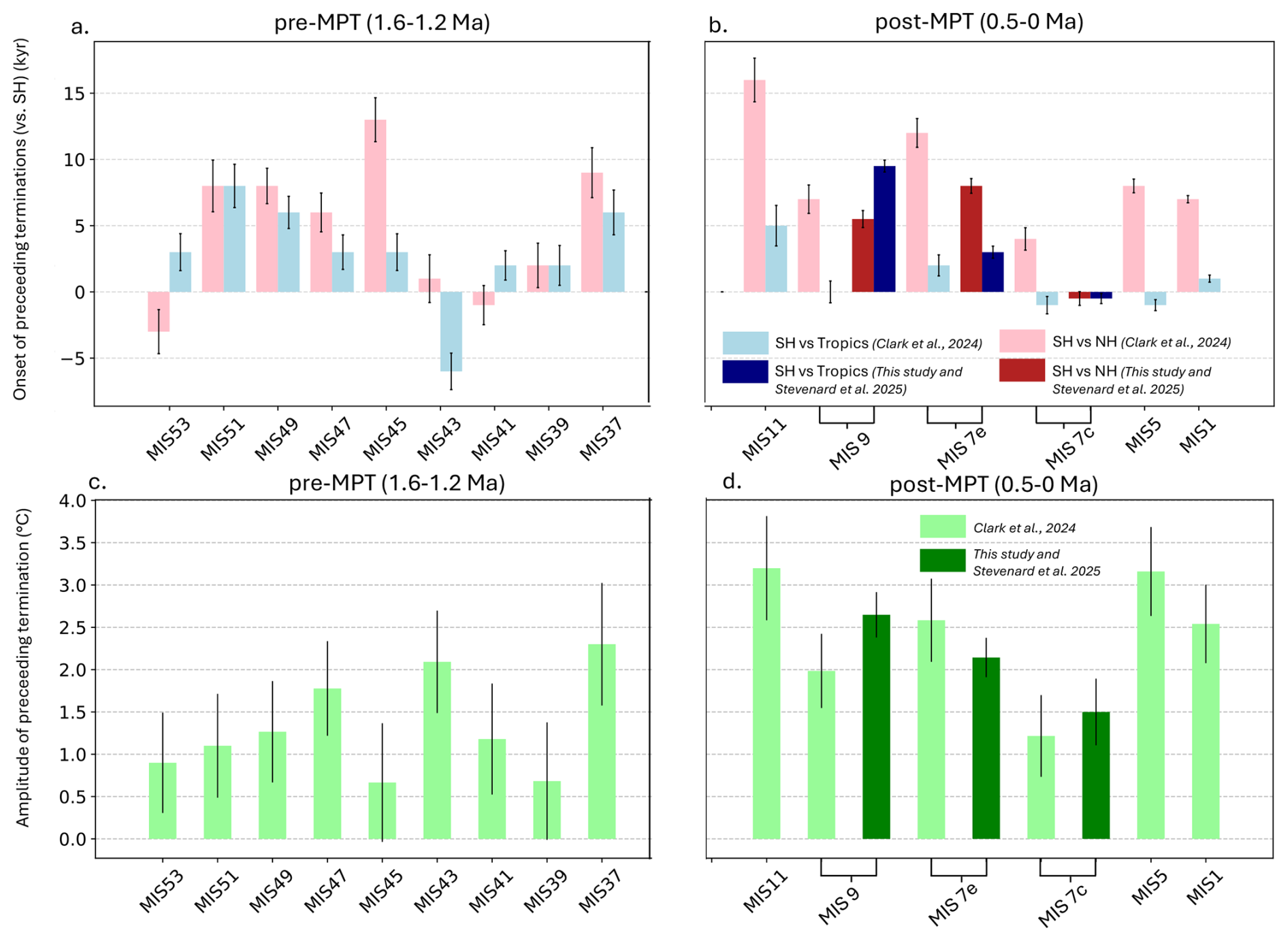
Figure 8 MIS 7 in the context of the post- and pre-MPT interglacials. Data are from Clark et al. (2024), excepted for MIS 7 (bold colors, this study) and MIS 9 (bold colors, Stevenard et al., 2025). (a) Timing of the onset of the preceding glacial termination between Southern and Northern Hemispheres stacks (pink) and between Southern Hemisphere and Tropics stacks (light blue), for the pre-MPT period (1.6–1.2 Ma). A positive value indicates an early onset of glacial termination in the Southern Hemisphere compared to the other stack. No value corresponds to a synchronous glacial termination onset. (b) Same as panel (a) but for post-MPT interglacials. (c) Temperature amplitude of the termination (green) based on GSST reconstruction. (d) Same as panel (c) but for post-MPT interglacials. Errors bars correspond to 1σ uncertainty.

Regarding termination mechanisms, previous studies have evidenced a key role of Agulhas Leakage over these periods (e.g. Caley et al., 2011; Nuber et al., 2023; Stevenard et al., 2025). During glacial terminations, a southward shift of the Southern Hemisphere westerlies enhances the Agulhas Leakage, increasing the inflow of warm, salty Indian Ocean waters into the South Atlantic. This would strengthen the Atlantic Meridional Overturning Circulation (AMOC), promotes interhemispheric heat exchange, and triggers early Southern Hemisphere warming that may accelerate global deglaciation (Caley et al., 2011; Nuber et al., 2023). The role of Agulhas leakage appears minor during TIIIa, as the only SST record from the Agulhas corridor shows no significant warming during this interval, contrary to during TIII (core MD96-2077, Fig. S3). As MIS 7d is shorter in duration than other glacial periods, it is likely that the Indian Ocean is not isolated long enough (Nuber et al., 2023) to produce the necessary warming to accelerate the glacial termination. This mechanism could explain why the early South Atlantic warming during TIIIa is imperceptible compared to TIII.

Watanabe et al. (2023) conducted sensitivity experiments with artificially reduced obliquity amplitude (to 60 % of modern values). Under this reduced obliquity scenario, their model produced 100 ka cycles over the early Pleistocene interval (1.6–1.2 Ma). In contrast, using the real full-amplitude obliquity produced the 41 ka pacing. These experiments demonstrate that the amplitude of obliquity alone can regulate the frequency of glacial cycles. Applying this framework to MIS 7, the exceptionally high obliquity peak synchronous with MIS 7c (Laskar et al., 2004; Past Interglacials Working Group of PAGES, 2016) may have temporarily shifted the climate system away from 100 ka eccentricity pacing and back into a 41 ka rhythm. This interpretation resonates with the self-sustained oscillation climate hypothesis (Mitsui et al., 2023). Simulations performed with an Earth system model of intermediate complexity evidences the existence of self-sustained climate oscillation at glacial-interglacial timescales, and develop the idea that the synchronization of such oscillation to orbital parameters may have driven major climate transition such as the MPT (Mitsui et al., 2023). Our results suggest that MIS 7c represents a temporary re-synchronization of the self-sustained climate oscillation with the obliquity forcing as it was the case during the 41 ka world period, temporarily overriding the prevailing 100 ka periodicity of the late Pleistocene.

Before MIS 7, two other interglacials of the Late Pleistocene, MIS 15 and in a lesser extent MIS 13, also exhibited a double warm peak structure (Past Interglacials Working Group of PAGES, 2016). These sequences are considered as the onset of 100 ka cycle occurring after the Mid-Pleistocene Transition, as it was preceded by the first extreme glaciation (MIS 16) of the Late Pleistocene. However, a comprehensive synthesis of surface temperature data for MIS 15 and MIS 13 remains unavailable. Unlike MIS 7, MIS 15 and MIS 13 did not occur under exceptional orbital forcing (Fig. 7) and took place in between the Mid-Pleistocene Transition and the Mid-Brunhes Shift (Past Interglacials Working Group of PAGES, 2016). Over this period, climate cycles were still shifting from a 41 ka to a 100 ka periodicity, resulting in interglacials including both periods signatures, restricting a direct comparison with MIS 7.

Although MIS 7 appears to have been paced by mechanisms reminiscent of the 41 ka glacial cycles, the warming pattern of TIIIa questions this comparison. TIII, which precedes MIS 7e, exhibits the classic characteristics of a glacial termination: deglaciation begins in the Southern Hemisphere at ∼ 254 ka, progresses to the Tropics by ∼ 251 ka, and finally reaches the Northern Hemisphere at 246 ka (Fig. 4d). This hemispheric progression is characteristic of the bipolar seesaw mechanism, whereby Southern Hemisphere warming leads Northern Hemisphere deglaciation through oceanic heat redistribution (Stocker and Johnsen, 2003), and of the role of the Agulhas leakage (Caley et al., 2011; Nuber et al., 2023; Stevenard et al., 2025). Such phasing pattern has already been observed for the youngest terminations (e.g. TI: Shakun et al., 2012; TIV: Stevenard et al., 2025).

In the Clark et al. (2024) synthesis, all terminations of the past 500 ka registered an early warming in the Southern Hemisphere compared to the Northern Hemisphere (Fig. 8b). In contrast, our results for TIIIa, which leads into MIS 7c, are marked by a near-synchronous SST rise across all latitudes, with no detectable interhemispheric phasing at the onset of warming (Fig. 8b). This globally uniform warming signal differs from the youngest terminations and suggests the involvement of other underlying dynamics, such as the role of the Agulhas Leakage (Stevenard et al., 2025; Fig. 8b). However, the analysis of recently published hemispheric SST stacks spanning the entire Pleistocene (Clark et al., 2024) reveals that a warming sequence characterized by an early Southern Hemisphere warming also appears to be a dominant feature of the 41 ka world. Some exceptions may occur during MIS 53 and MIS 41 (Fig. 8a), but chronological uncertainties for this interval remain large, and the analyses rely on only a small number of records (Clark et al., 2024).

The deviation of TIIIa from classical Pleistocene glacial terminations suggest that MIS 7 was not a return to pre-MPT dynamics, but rather a manifestation of 100 ka climate cyclicity operating under extreme obliquity conditions. As such, MIS 7 represents a hybrid interglacial, embedded within the post-MPT 100 ka framework, yet shaped by obliquity-driven forcing typical of the early Pleistocene.

5 Conclusions

This study presents the first comprehensive global-scale synthesis of SST focusing on TIII and MIS 7 including 132 high-resolution SST records aligned on a common chronological framework (i.e. the AICC2023 ice core chronology). Based on local, regional and global analyses of surface temperature variations, our results show that:

• Regional temperature stacks evidence a pronounced regional variability during MIS 7: across ocean basins, the structure can range from a well-defined pattern with three distinct temperature peaks corresponding to warm substages MIS 7e, 7c, and 7a (e.g., North Atlantic), to a more subdued signal characterized by low-amplitude of variations (e.g., Equatorial Pacific).

• Hemispheric temperature stacks revealed a heterogeneity in magnitude of the different warm and cold stages of MIS 7. While the Southern Hemisphere indicates an optimum during MIS 7e, the Northern Hemisphere and the Tropical areas reach their temperature maxima during MIS 7c.

• At the global scale, MIS 7c appears comparable to, or slightly warmer than MIS 7e. Global mean surface temperatures during both MIS 7e and MIS 7c remain below PI values (ΔGMST = −1.4 ± 0.3 and −1.0 ± 0.3 °C, respectively).

• The global mean surface temperature over MIS 7e and MIS 9e.evidences a transient decoupling with atmospheric CO₂ concentrations during periods of CO₂ overshoots.

• Our results reveal that, while TIII displays the classical structure of a glacial termination characterized by a hemispheric phasing consistent with the bipolar seesaw hypothesis, TIIIa is marked by a near-synchronous SST rise across all latitudes, suggesting a distinct underlying mechanism.

Based on these key results and comparative analyses, our study highlights the unique character of MIS 7, situated within the 100 ka world yet exhibiting features uncharacteristic of late Pleistocene interglacials. We propose that MIS 7 represents a brief and temporary re-synchronization of internal climate oscillations with the 41 ka obliquity cycle, driven by the unusually extreme obliquity values reached during this interval. Rather than being a strict analogue of the early Pleistocene 41 ka world, MIS 7 should be viewed as a hybrid interglacial, resulting from the occurrence of specific orbital context within the post-MPT world.

Beyond the characterization of MIS 7, this synthesis represents a unique accessible dataset that compiles SST records with up-to-date methods that have been aligned on a common chronology. This effort provides a benchmark to evaluate Earth System Model simulations that have been performed over this period. Data-model comparison would help disentangling the role of greenhouse gases variations, oceanic dynamics and orbital forcing in shaping the unique morphology of surface temperature changes over MIS 7.