On the implementation of external forcings in a regional climate model – a sensitivity study around the Samalas volcanic eruption in the Eastern Mediterranean/Middle East

Natural and human-historical archives document regional climate variations and extremes of the past 2500 years across the Eastern Mediterranean/Middle East. Earth System Models (ESM) can contribute to the interpretation of the variations in the paleoclimate data and the dynamics of the underlying mechanisms. State-of-the-art ESMs have a good temporal resolution but are spatially too coarse to adequately address regional processes. Here, we provide for the first time a regional climate model (RCM) output adjusted to past climates forcings covering the Eastern Mediterranean/Middle East at a 0.44° horizontal and up to hourly temporal resolution. CMIP6 external climate forcings of volcanic, orbital, solar and greenhouse-gas changes are implemented in the RCM COSMO-CLM (CCLM, COSMO 5.0 clm16). The sensitivity of the model to each of the implemented forcing is tested separately and in combination in a case study around the large Samalas volcanic eruption (1255–1264 CE) with strong socio-economic impacts in the study area. We evaluate the impact of the different implemented forcings compared with the standard CCLM model version for the present time. The orbital forcing is found to have the largest effect with cooler winter/spring and warmer autumn during the test period. The volcanic forcing has a strong cooling effect for a couple of years after the large volcanic eruption. Other climate forcings only show a smaller impact in the sensitivity study, while the improvements in simulated precipitation are mainly due to the higher spatial resolution than to a specific forcing. The study is the basis for the new 2500-year-long transient, fully forced RCM simulation. It offers an assessment of the implementation of forcings in the RCM, along with an enhancement of the simulations' skill through the use of the RCM. We aim to enhance our understanding of the role of single and joint forcings on climate variability and extremes, their underlying processes at the regional scale, potential climate-society interactions and address limitations and uncertainties.

1 Introduction

Earth System Models (ESMs) are powerful tools that combine the complex interactions of physics, chemistry and biology of Earth systems and contribute to a better understanding of processes in and between its spheres. Various ESMs with a standard resolution of 1.9° (approximately 200 km in the atmospheric component) are used to investigate specific periods of the past, present, and future (Giorgetta et al., 2013). The Coupled Model Intercomparison Project Phase 6 (CMIP6) is a collaborative initiative within the climate science community aimed at advancing our understanding of the Earth's climate system (Eyring et al., 2016). Systematic experiments conducted within CMIP6 include the study of past climate conditions, projections of future climate and climate sensitivity, refinement of model performance, validation of models and provision of data to support decision-making. The Paleoclimate Modeling Intercomparison Project (PMIP) was established with the aim of investigating the influence of forcing and feedback on the climate system and comparing climate model simulations with paleoclimate reconstructions and observations (Williams et al., 2020, 2021; Lunt et al., 2021) and is under CMIP6 in its fourth phase (PMIP4) (Kageyama et al., 2018).

The CMIP6/PMIP4 simulations have a large grid size of 200×200 km, thus 400 km² with the exact same climate conditions. This poses considerable challenges for research on the regional climate in areas of complex topography, such as mountainous or coastal regions. Additionally, it complicates comparison with proxy data, which often has limited spatial coverage and representation. Moreover, integrating these outputs into impact studies becomes even more challenging (e.g. Phipps et al., 2013; Xoplaki et al., 2018). To address the limitations of coarse ESM simulations for regional climate analysis, researchers apply statistical and/or dynamical downscaling techniques. Dynamical downscaling employs high-resolution models to capture regional features, while statistical downscaling leverages relationships between large-scale variables to enhance spatial resolution. The PALEOLINK working group of the PAGES (Past Global Changes; https://www.pastglobalchanges.org, last access: 21 February 2025) network has identified both approaches as scientific goals (Gómez-Navarro et al., 2019). Ludwig et al. (2019); Gómez-Navarro et al. (2015a, b, 2019) demonstrate that regional climate simulations obtained through dynamical downscaling can enhance the comparability between climate model output and paleo climatic evidence at the regional scale. Furthermore, Armstrong et al. (2019) found improved climatology of regional climate simulations compared to global climate simulations in the Northern Hemisphere for the millennium preceding the industrial era (past1000), the mid-Holocene around 6000 years ago (midHolocene) and the Last Glacial Maximum around 21 000 years ago (lgm). High-resolution RCM simulations offer detailed insights into general and regional atmospheric circulation patterns (Cortina-Guerra et al., 2021). Such simulations have been used to investigate the interaction between different regional climates and other spheres (e.g. Ludwig et al., 2017, 2018, 2021; Ludwig and Hochman, 2022; Russo et al., 2024; Schaffernicht et al., 2020; Velasquez et al., 2021, 2022) during the lgm with the Weather Research and Forecasting Model (WRF). Additionally, RCMs assist in interpreting proxy data, as illustrated by Pinto and Ludwig (2020). RCM simulations also facilitate consistency analysis of gridded reconstructions, demonstrated by Gómez-Navarro et al. (2015a, b).

The low-resolution ESM used to drive the RCM, significantly impacts the high-resolution simulations. To mitigate this influence, external climate forcings from the ESM can be implemented directly in the RCM. This approach enables a more direct effect of the forcings on the RCM simulation, reducing dependence on the ESM and enhancing understanding of their effects on the regional climate (Prömmel et al., 2013). The relevance of various external climate forcings for climate variability depends on the period under consideration. The forcings that are important over the last 2500 years are the same as in the CMIP6/PMIP4 past1000 experiments, which are the orbital, solar, volcanic, greenhouse gas and land-use changes (Jungclaus et al., 2017). Those forcings have not yet been explicitly implemented in standard regional climate models. Here, we implemented them in the COSMO-CLM model (Rockel et al., 2008). This method leads to the creation of a novel, detailed paleo-regional climate model (paleo-RCM). To investigate the effects of various climate forcings, a set of decade-long sensitivity experiments is conducted. Simulations are performed with individual forcings applied separately, as well as with combined forcings, and compared to a reference simulation calibrated to present-day conditions. This approach enables the evaluation of the relative contributions of external forcings and internal variability to observed changes (Otto-Bliesner et al., 2016). The RCM is driven by the fully forced PMIP-conform MPI-ESM-LR simulation to isolate the additional effect of implementing the forcings into the RCM. This study aims to assess whether incorporating external forcings into the RCM enhances the realism of regional-scale simulation output. To achieve this, differences between sensitivity experiments (using single and combined forcings), the MPI-ESM-LR, and the reference CCLM simulation are analyzed.

Periods of high volcanic activity are prominent candidates for conducting sensitivity experiments over the last few millennia. Specifically large volcanic tropical eruptions exert impacts on the global and regional climate. In this context, the 12th and 13th centuries are notably active periods (Guillet et al., 2023 and reference therein). The eruption of the Samalas volcano on the Indonesian island of Lombok in 1257 stands out as the 5th largest volcanic eruption of the last millennium in terms of sulfate deposition (Lavigne et al., 2013; Guillet et al., 2017, 2023) and in terms of the emissions stands as the greatest volcanogenic gas injection of the Common Era (Vidal et al., 2016). With a Volcanic Explosivity Index of 7, it ranks as one of the most significant eruptions in history (Whelley et al., 2015). Consequently, the Northern Hemisphere experienced some of the coldest summers of the past millennium in the years 1258 and 1259 (Guillet et al., 2017). These climatic shifts combined with societal vulnerabilities have been linked to historical instances of agricultural deficits, civil unrest, pestilence, and migration (e.g. Post, 1977; Oppenheimer, 2011; Luterbacher and Pfister, 2015; Guillet et al., 2017, 2023; Malawani et al., 2022). The effects of the Samalas eruption were felt throughout the Mediterranean and contributed to considerable cooling and existential crises in various regions (e.g. Xoplaki et al., 2016, 2018, 2021; Guillet et al., 2020, 2023; Malawani et al., 2022). The cumulated impact of these events has been suggested as a contributing factor to the onset of the Little Ice Age (Miller et al., 2012).

We focus on the Eastern Mediterranean and the Middle East (EMME, Zittis et al., 2022), which includes the Eastern Mediterranean, North-East Africa, the Arabian Peninsula, and the Middle East. Cultures and societies that flourished in this area, such as Ancient Egypt, Ancient Greece, and Ancient Rome, had a profound influence worldwide (Wilson, 2013; Sallares , 1991; Feldman, 1991). These societies expanded their reach beyond Europe, extending along the Nile River, the Red Sea, and toward the Caspian Sea and the Persian Gulf. Given the extensive history of developed cultures, abundant historical data and proxy records are available in this region. In addition, the area is recognized as a climate change hotspot (Giorgi, 2006; Lelieveld et al., 2012, 2016; Cramer et al., 2018; Zittis and Hadjinicolaou, 2017; Zittis et al., 2019, 2022), making it particularly compelling for climatic studies.

Conceptually, the study falls into the category of an external parameter-sensitivity experimental setup. Using a combination of ESM and RCM models, one can either use an ensemble of different ESM simulations with an undisturbed or default parameter setting in the regional model, or change the external forcing parameter space in RCM simulations with a single ESM simulation. In the ensemble setup, one can explore the amount of natural variability the ESM brings to the RCM, in addition to changes caused by external forcings. One variant of this approach uses different versions of ESMs to force a single RCM (cf. CORDEX). In this study, we explore the effects of implementing different external forcings into the RCM to test the impact of individual forcings in RCM simulations (see also the motivation in Ludwig et al., 2019). The primary aim of this study is not to decipher the amount of external versus internal variability in the simulated climate, but rather to demonstrate the impact of adding individual forcings to the portfolio of external forcing parameters in the RCM.

The structure of this study is organized as follows: Sect. 2 details the models, their configurations, and the implemented forcings. The described methods, in general, apply to the entire 2500-year period but are specifically tailored for our target period, the Samalas volcanic eruption selected as a sensitivity study. Section 3 focuses on the sensitivity analysis for the Eastern Mediterranean and Middle East during the Samalas period. It presents and interprets simulated temperature and precipitation data, including comparisons with the ESM, along with annual, seasonal, and monthly distributions. In Sect. 4, we present the main conclusions and outline potential directions for future research.

2 Material and Methods

2.1 Period and Domain

We focus on one of the largest volcanic eruptions of the last millennium, which was the Samalas eruption in 1257. Besides the enormous sulfate deposition and high emissions, the eruption created a 6–7 km wide caldera, known as Segara Anak, replacing the former Samalas mountain (Rachmat et al., 2016). Volcanic aerosols in the stratosphere, measured by the aerosol optical depth (AOD), sharply increased after the eruption and remained elevated for several years, as illustrated in Fig 1, a reconstruction of Toohey and Sigl (2017) for a wavelength of 550 nm (visible light). The substantial amounts of volcanic sulfate aerosols led to stratospheric warming and surface cooling (Robock, 2000; Crowley et al., 2008). In our study, we focus on the decade spanning 1255–1264 CE which includes the Samalas eruption in 1257, as a test case for conducting sensitivity experiments.

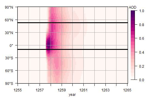
Figure 1 AOD from 1255 to 1265 for the different latitudinal bands. The latitudes used for the simulations are between the bars. Own representation of data from Toohey and Sigl (2017).

The simulations cover a domain similar to MENA-CORDEX (Zittis et al., 2014), with a focus on the EMME (Zittis et al., 2022) – a region rich in historical significance. The EMME is of interest not only in terms of history and society but also in terms of climate, which may be closely linked to historical and societal developments and changes (Crowley and North, 1988; Holmgren et al., 2016; Izdebski et al., 2016).

2.2 MPI-ESM-LR

We performed a global simulation using the MPI-ESM-LR (Giorgetta et al., 2013) in version MPI-ESM1.2.01p5, which is a new realization of the transient MPI-ESM simulation following the CMIP6-protocol for PMIP4 past1000 simulations by Jungclaus et al. (2017). To suit the requirements of the regional climate model COSMO-CLM, the output intervals are adjusted accordingly with variables written out at a 6 h resolution. The MPI-ESM-LR comprises the coupled general circulation models for the atmosphere – ECHAM6 (Stevens et al., 2013) and the ocean – MPIOM (Jungclaus et al., 2013), along with the subsystem models for land and vegetation JSBACH (Reick et al., 2013; Schneck et al., 2013) and marine biogeochemistry HAMOCC5 (Ilyina et al., 2013). Atmospheric and vegetation-related variables in particular are essential inputs for the regional climate simulation. The spatial resolution of the simulation is 1.875° which is approximately equivalent to 200 km (T63). More details on the model version and configurations can be found in Mauritsen et al. (2019).

2.3 COSMO-CLM

The regional climate simulations are performed with the regional climate model COSMO-CLM (Rockel et al., 2008), which is the model developed by the COnsortium for Small-scale MOdelling (COSMO) in CLimate Mode (Baldauf et al., 2011; Rockel et al., 2008) and is further developed by the CLM-Community. In this study, the COSMO model version 5.0 with CLM version 16 (COSMO-CLM-v5.0_clm16) is used. The model is forced by a transient MPI-ESM-LR simulation (Jungclaus et al., 2017) and the interpolation from the forcing data to the model is performed using INT2LM version 2.05 with CLM version 1 (INT2LM-v2.05_clm1) (Schättler and Blahak, 2017). Time integration is achieved using the two time-level Runge-Kutta scheme (Jameson et al., 1981) with a model time step of 300 s. Convection parameterization is based on the Tiedtke scheme (Tiedtke, 1988). The representation of albedo and aerosols, identified as crucial parameters by Bucchignani et al. (2016), are set according to their values. The land surface model is TERRA-ML (Doms et al., 2011; Schulz et al., 2016). The external data set is prepared using EXTPAR (Smiatek et al., 2008). These settings remain consistent for all experiments, facilitating a pure sensitivity study solely focused on differences attributable to external forcings.

The simulations are carried out for a domain including the Eastern Mediterranean, the Middle East and the Nile River basin from Lake Victoria to the Delta (Lon =4–60° E, Lat =5° S–49° N). In this study, only the EMME region is analyzed (Lon =18–60° E, Lat =12.5–42.5° N). The simulation and the analyzed domains are shown in Fig. 2 with a mesh size of 0.44^∘ (∼ 50 km), which was in tests found to be appropriate (Hartmann et al., 2024). Each experiment spans the period from 1255 to 1264 CE.

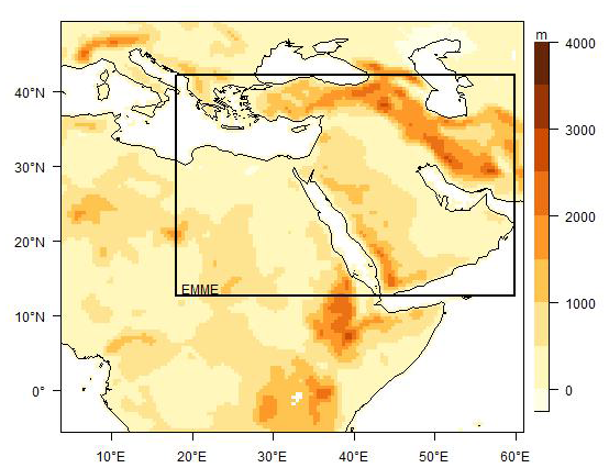
Figure 2 Simulation domain with topography and the EMME region in the black rectangle.

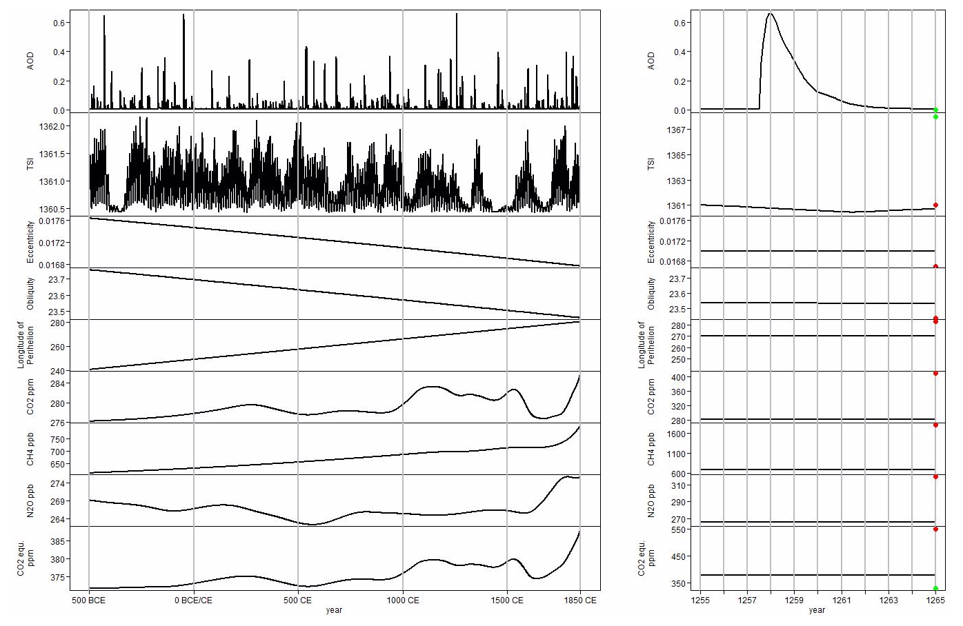
Figure 3 Transient forcings for two distinct periods: 500 BCE to 1850 CE (left) and 1255–1265 CE (right). Present-day value (2020 CE) is denoted by a red dot, and the value utilized in the reference COSMO-CLM simulation by a green dot (AOD, TSI, CO₂-equivalent). The components of the forcings are as follows: Aerosol Optical Depth (AOD) by Toohey and Sigl (2017) representing volcanic forcing, Total Solar Irradiance (TSI) by Jungclaus et al. (2017) representing solar forcing, Eccentricity, Obliquity and Longitude of Perihelion by Berger (1978) representing orbital forcing and Effective CO₂ (CO₂, CH₄ and N₂O) representing greenhouse gas forcing (Meinshausen et al., 2017).

2.4 External Climate Forcings

The external forcings are defined based on the recommendations for the PMIP4 past1000 contribution to CMIP6 (Jungclaus et al., 2017). These forcings include time-varying parameters. Orbital forcing is crucial for long time scales spanning centuries to millennia (Rial and Anaclerio, 2000; Cubasch et al., 2006). Solar, greenhouse gas and land-use change forcings exhibit effects within decades, albeit indirectly, leading to a comparably slower climate response (Cubasch et al., 2006). In contrast, volcanic forcing has a direct strong, rapid and short-term impact (Wigley et al., 2005) and up to decadal climate effects through secondary processes (Stenchikov et al., 2009; Shindell et al., 2009; Otterå et al., 2010; Zanchettin et al., 2012; Swingedouw et al., 2015; Kremser et al., 2016). The volcanic forcing is described by variations in aerosol optical depth (AOD) at a wavelength of 550 nm by Toohey and Sigl (2017). AOD is the only climatic forcing significantly varying during the simulated period, with the eruption in 1257 registering as a prominent peak of AOD, one of the largest in the Common Era (Fig. 3). The solar forcing is represented by changes in the total solar irradiance (TSI), which is influenced by sunspots and faculae directly on the sun's surface by the SATIRE reconstruction data set (Jungclaus et al., 2017). The present-day TSI values closely match those used in the Samalas case study and exhibit minimal variability over the ten years, as depicted in Fig. 3. In contrast, the TSI value used for the reference simulation differs significantly from the Samalas period values due to the specifications of the CCLM model for present-day conditions. Orbital forcing is represented by the eccentricity, the obliquity and the longitude of perihelion, varying on time scales of dozens to hundreds of millennia. A static implementation of orbital forcing initially prepared by Patrick Ludwig (personal communication, 2020) is extended throughout this study. Annual data is provided by Berger (1978). Compared to the mid-13th century, today's orbit exhibits slightly lower eccentricity and obliquity, and higher precession. Figure 4 illustrates the cumulative effect of these factors on insolation during the 13th century (1250 CE) compared to the present (1950 CE, reference configuration). In the Eastern Mediterranean and Middle East (EMME) region, this translates to lower insolation from December to June during the 1260s, while July to November experienced higher insolation compared to the present. GHG concentrations encompassing CO₂, CH₄ and N₂O are implemented via equivalent CO₂, all obtained from (Meinshausen et al., 2017). It is noteworthy that the CO₂ concentration in the reference simulation (330 ppm) is lower than the combined effective CO₂ utilized in the transient GHG forcing as illustrated in Fig. 3. In this study only results for the sensitivity period (1255 to 1264 CE) are presented, but Fig. 3 also shows the evolution of the external climate forcings over the last 2.5 millennia to illustrate and contrast the long- and short-term changes in individual forcings.

The choice of land-use data source significantly influences atmospheric conditions (Zhang et al., 2021). The CCLM cannot differentiate between various land cover types except for deciduous and evergreen forests and tends to overestimate the effect of the shrubs and grass due to every plant following the same phenological cycle (Hartmann et al., 2020). To address this limitation, a transient land-use dataset based on global JSBACH output was implemented in the CCLM. Although not utilized in this study to avoid confounding the influence of other forcings, details about the land-use forcing can be found in Appendix A since a transient land-use forcing is used in our simulation of the last 2500 years. Other potential forcings such as ice sheets or tropospheric aerosols are not specifically implemented from external datasets in either the CCLM or MPI-ESM-LR. External forcings used in CMIP6 for other historical periods could similarly be incorporated into the CCLM to enable high-resolution simulations of these periods, depending on the scientific interest.

Table 1 Experiments. The MPI-ESM-LR is the driving model, “REF” is the CCLM simulation with standard configuration, “ORB/SOL/VOL/GHG” are the simulations with the respective forcing only and “FULL” is the simulation with all forcings combined. Values for “transient” can be seen in Fig. 3. “solc” is short for solar constant. Transient values are during the ten-year study period approximately: CO₂-equivalent =378 ppm, solc =1361 W m⁻², AOD-max =0.6638, eccentricity =0.017, obliquity =23.54, perihelion =270. Present-day orbital values are eccentricity =0.0167, obliquity =23.44, perihelion =282.

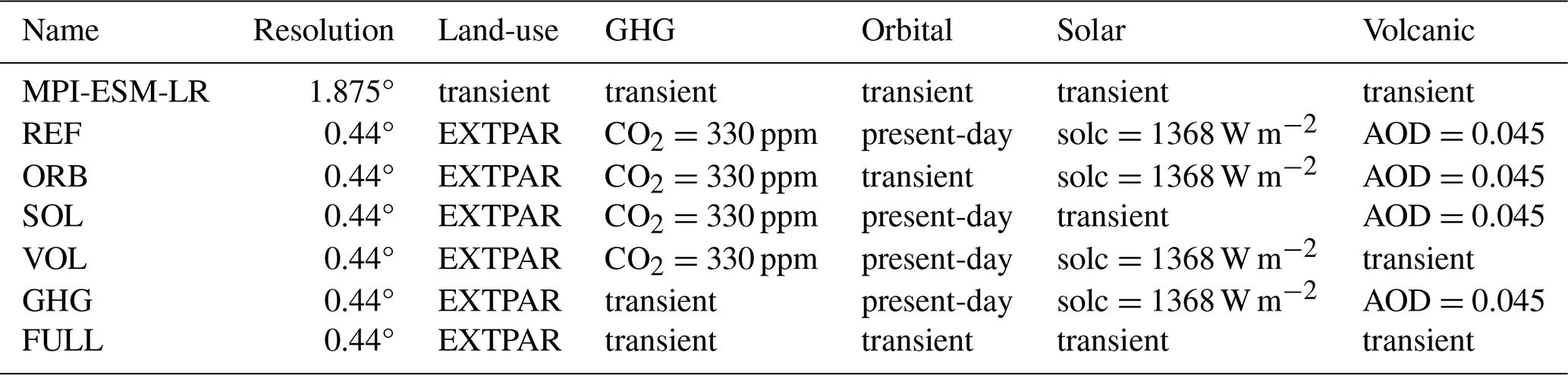
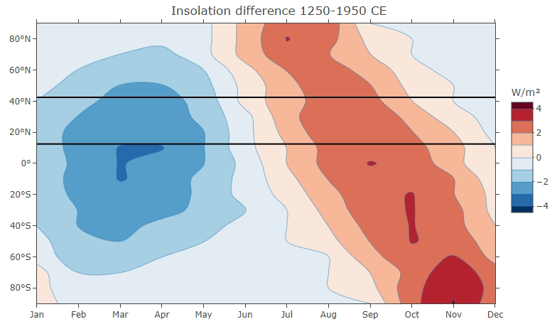
Figure 4 Insolation difference due to orbital forcing between the century of the Samalas eruption and present days (1250–1950 CE; own representation of data from Berger and Loutre, 1991 linearly interpolated). The study domain is between 12.5 and 42.5° N marked with horizontal lines.

2.5 Experiments

To investigate the influence of different forcings on the climate across the EMME region from 1255 to 1264, we conducted simulations using single forcings and their combination, comparing them with the CCLM standard configuration. The CCLM standard configuration, tuned for present-day climate serves as the reference simulation (REF). The CCLM is configured for simulations of the present with the possibility of historical runs from the 20th century all the way to future projections with known concentration pathways. Notably, all experiments use the same boundary forcing of the fully forced ESM simulation, precluding individual forced sensitivity studies for the ESM. All RCM simulations employ EXTPAR external land-use data and share the same horizontal and temporal resolution and settings, except for the forcing data. Our reference simulation maintains fixed values for GHG concentration (330 ppm), TSI (1368 W m⁻²) and stratospheric AOD (0.045). The GHG concentration was the default value for the German Weather Service, while the solar irradiance and the optical depth are empirical values. The orbital forcing is not explicitly addressed by the model and is designed for present-day simulations (eccentricity =0.0167, obliquity =23.44, perihelion =282). Explicit values of the forcings are summarized in Table 1, while details of the transient forcings are depicted in Fig. 3. For the sensitivity simulations, the orbital, solar, volcanic and GHG forcings are implemented in a transient mode using the introduced datasets. Each forcing is individually incorporated into the CCLM source code, enabling direct assessment of their influence on the simulated climate. For the fully forced simulation, all transient forcings are combined, ensuring consistency between the global ESM and the high-resolution RCM. This approach aims to yield the most realistic results.

3 Results and Discussion

3.1 2 m Temperature

3.1.1 Comparison ESM – RCM

The higher resolution of CCLM, compared to the MPI-ESM-LR, allows for a more detailed depiction of topographic features, including coastlines and complex mountain ranges. Figure 5 illustrates the decadal mean 2 m temperature and standard deviation of the MPI-ESM-LR and the CCLM models for the period 1255–1264 CE. While there is a similar overall pattern across all simulations, CCLM captures more detailed features in mountainous regions and along the Mediterranean/Black Sea coast. The temperature distribution is influenced by orography in both model simulations, with higher heterogeneity in CCLM due to its higher resolution. Profound differences are observed in regions such as the Red Sea and Caspian Sea coasts, where the CCLM simulation shows lower temperature values compared to MPI-ESM-LR. Both models present lower standard deviations over the Arabian Peninsula and the Middle East, while the RCM emphasizes higher variability over land compared to sea regions. In summary, while the overall patterns of 2 m temperature in the ESM and RCM simulations are generally consistent, substantial differences arise in areas with complex terrain, which are prevalent throughout the EMME region.

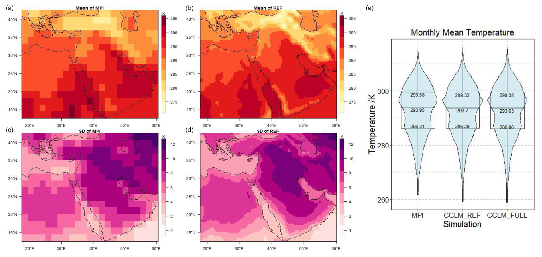
Figure 5 Decadal mean (a, b) and standard deviation (c, d) of 2 m temperature in K for the period 1255 to 1264 in the driving MPI-ESM-LR (a, c) and the fully forced CCLM (b, d) and violin plot together with boxplot of the monthly mean 2 m temperatures across the full EMME domain and decade (e, values are upper quartile, median, lower quartile).

The violin plot on the right side of Fig. 5 displays all monthly mean temperatures across the entire EMME domain for the 10 years. Notably, the higher resolution leads to an increased frequency of cold temperatures, which can be attributed to elevated regions where lower temperatures are better captured due to the more detailed representation of orography. The better representation of lower temperatures over orography is due to the lapse rate effect. The temperature follows a bimodal distribution with the major mode between the median and the upper quartile and the minor mode close to the lower quartile. This is indicated by the two climate classifications mainly represented in this large domain, which are the hot arid desert climate in the Sahara and the Arabian Peninsula and the warm temperate summer dry climate in the Mediterranean (Kottek et al., 2006). The lower quartile values presented in the box plot and the violin plot on the right side of Fig. 5 indicate that the fully forced RCM model (FULL) exhibits even more extreme temperatures than the standard (REF) configuration. In comparison to the MPI-ESM-LR simulation, the quartile values of the REF and the FULL simulation are between 0.25 and 0.32 K cooler, indicating a general shift towards cooler temperatures when using the RCM. Further clarifications regarding the differences between the CCLM simulations will be discussed in subsequent sections.

3.1.2 Annual and Seasonal Distribution

A major volcanic eruption such as the Samalas in 1257 CE releases substantial amounts of sulfate aerosols into the stratosphere, inducing large-scale surface cooling (Robock, 2000). This cooling effect persists as long as the additional volcanic aerosols remain present and physically active in the stratosphere. Figure 6 presents the post-eruption cooling observed in the mean annual temperature over the EMME region. Generally, the RCM simulations are in good agreement with the driving MPI-ESM-LR. In 1258, the annual mean temperature was more than 1 K cooler than in 1257. By 1259, the concentration of the stratospheric aerosols began to decline again (see also Fig. 1), initiating a gradual return to pre-eruption temperature levels between 1260 and 1263. This observed pattern is in agreement with proxy-based and historical records, as documented by Guillet et al. (2017) and those specific to the EMME region by Xoplaki et al. (2018, 2021). The post-eruption cooling is physically meaningful, but given the 1 K cooling prior to the eruption (1255 to 1256), it is not significant if only this one decade is considered. This issue will be addressed in future studies involving a multi-century transient simulation. Another way to rule out the possibility of natural variability would have been to run an ensemble of simulations for each experiment. However, limited resources made this impossible. Here, we focus on the differences between the implemented forcings in single runs.

In the right part of Fig. 6, the differences among the sensitivity experiments with respect to the reference simulation (REF) are shown. The VOL and FULL simulations represent the lowest temperatures as they are most influenced by the volcanic eruption with direct implementation of the volcanic forcing. Although all CCLM simulations receive information about the volcanic eruption from the driving ESM at the boundaries, only VOL and FULL explicitly account for the decrease in AOD caused by the volcanic eruption within their radiation routines. It is therefore worth noting that in the years following the volcanic eruption, these two experiments correspond particularly well with the MPI-ESM-LR. In 1258, the first year after the eruption, the annual mean temperature in the FULL and VOL simulations was more than 1.5 K cooler than before the eruption and about 0.4 K cooler than the REF simulation. By 1259, the second year after the eruption, the temperature differences started to decrease, with less than 0.2 K difference, and nearly disappeared in the subsequent years. Across all simulations, the annual mean 2 m temperature remains below the pre-eruption value until 1262. This suggests that the direct implementation of the volcanic forcing in the radiation routine of CCLM offers the most significant impact during the initial months up to two years following the eruption, aligning with paleo climatic evidence from the region (e.g. Xoplaki et al., 2018, 2021). The other sensitivity experiments exert a smaller influence on the annual mean temperature compared to the REF simulation. The GHG simulation shows slightly higher temperatures, while the ORB and SOL simulations reveal slightly lower 2 m temperatures compared to the REF simulation. The small differences between GHG and SOL compared to REF can be attributed to the slightly higher effective CO₂ (330 vs. 378 ppm) and lower TSI (1368 vs. 1361 W m⁻²) of the implemented forcings compared to the values of the REF simulation, respectively. The difference due to orbital forcing stems from the shift between the 20th-century orbital settings in REF and the 13th-century values in the ORB and FULL simulations. Clearer and more reliable results could have been achieved with a larger set of simulations, which were not carried out due to limited resources. In summary, the FULL simulation reproduces the lowest temperatures during the studied decade as the effects of the different forcings are aggregated. In this context, the positive temperature anomalies due to the GHG forcing are outweighed by the negative temperature anomalies due to solar, orbital, and most importantly, volcanic forcing.

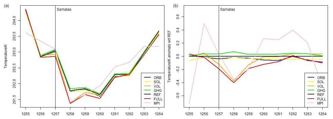
Figure 6 Annual mean 2 m temperature averaged over the EMME domain (a) for the CCLM simulations with the different forcings and the MPI-ESM-LR and the same values represented as anomaly (b) with respect to the reference CCLM from 1255 to 1264.

The spatial distribution of annual means (Fig. B1), corresponding to the right side of Fig. 6, reveals no unexpected or significant variations. Across most of the domain, temperatures are between 0.5 and 1 K cooler, with the VOL and FULL simulations for the year 1258, following the Samalas volcanic eruption, showing the most pronounced differences compared to the REF simulation (as detailed in Fig. B1 in Appendix B). Spatial differences between the SOL, ORB, and GHG simulations compared to the REF simulation are minimal, with a few exceptions occurring in specific years, areas, and simulations, showing no consistent pattern.

Figure 7 presents the seasonal mean 2 m temperature of the different experiments in comparison to the seasonal mean 2 m temperature of REF. In the FULL and ORB simulations, the differences are largest with up to 1.5 K and only here statistically significant according to a Wilcoxon-Test/Mann-Whitney-U-Test (α=0.05). The orbital forcing induces pronounced negative temperature anomalies during winter and spring over all land areas, attributed to the reduced insolation (see Fig. 4). The largest and partly statistically significant differences (more than 1 K cooler) are observed in spring over Mesopotamia and the Arabian Peninsula for the ORB and FULL simulations. In winter, the temperature differences are smaller, statistically significant only in the FULL simulation, and more pronounced in southern regions such as Arabia and the Sahara. In summer, the ORB simulation, along with the FULL and GHG simulations to a lesser extent, shows higher temperatures in the northern part of the domain and cooler temperatures in the south. In autumn, temperature anomalies in the ORB and FULL simulations are statistically significant and positive across all land areas, driven by increased insolation (as shown in Fig. 4). Deviations exceeding 1 K are most prominent over the Sahara and the Arabian Peninsula. In contrast, the SOL, VOL and GHG simulations show only minor, non-statistically significant temperature anomalies, ranging from slightly negative to positive values below 0.5 K, which is within the range of natural variability. The FULL simulation represents a combination of all individually forced simulations, with orbital forcing playing a dominant role in shaping seasonal temperature patterns. The simulations with implemented orbital forcing (ORB, FULL) show cooler winters and springs but warmer summers and autumns over almost the entire domain compared to the REF simulation. Since the REF simulation reflects 1950 CE orbital parameters, comparing simulations with implemented orbital forcing (ORB, FULL) with REF is equivalent to comparing 13th vs. 20th century climate conditions. Over these centuries, the gradual changes induced by orbital forcing accumulate and can reach several W m⁻². Since our domain is primarily situated in the subtropics, which are substantially less affected by atmospheric circulation compared to mid- and high-latitudes, the direct impact of orbital forcing, particularly on 2 m temperature, is understandable.

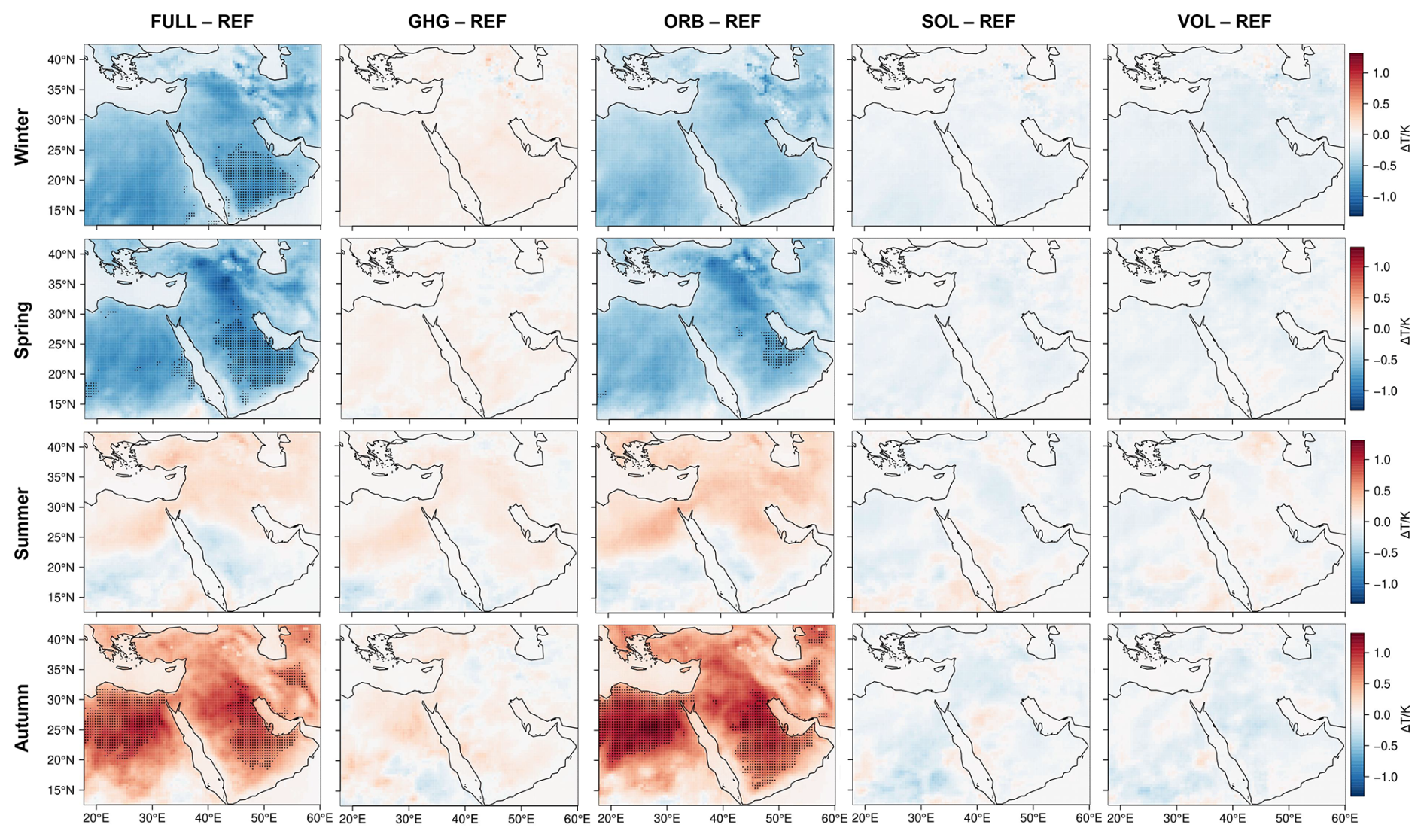
Figure 7 Mean seasonal temperature for the decade 1255–1264 for the different experiments compared to REF. Significant differences are marked with a dot (Wilcoxon-test, α=0.05). From left to right – FULL, GHG, ORB, SOL, VOL and top to bottom – winter, spring, summer, autumn.

3.1.3 Monthly Means – Distribution and Extremes

RCMs have, due to their higher spatial resolution, a higher ability to produce extreme events and values than ESMs (see Fig. 5). To study the influence of different forcings on these extremes, we examine the distributions of monthly mean 2 m temperature for the various simulations in each grid box and month within the EMME domain and decade, as illustrated in Fig. 8. The shape of the distributions remains consistent across all simulations, indicating similar average and quantile values for temperature. The medians and upper quartiles only slightly vary with values between 293.63 K in FULL to 293.75 K in GHG simulations, respectively, 299.28 K in SOL to 299.4 K in ORB simulations. Although the lower quartiles exhibit a greater spread, the simulations remain compatible, ranging from 286.06 K in FULL to 286.33 K in GHG.

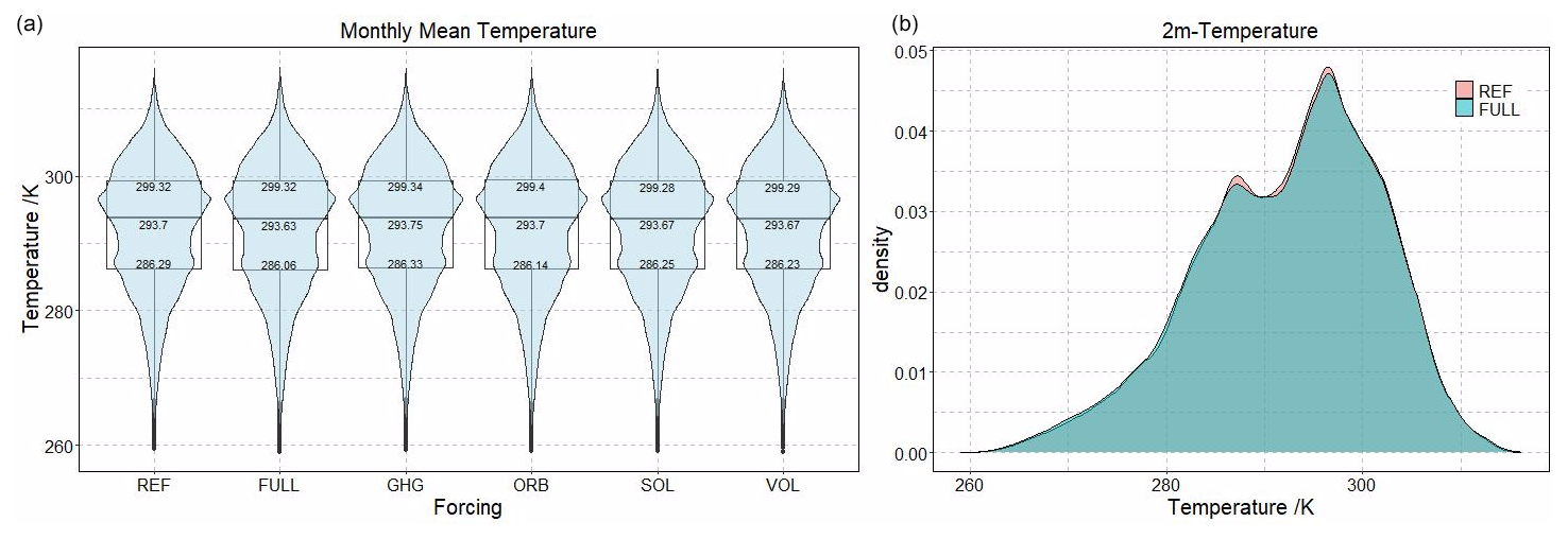
Figure 8 Violin plot and boxplot (a, values are upper quartile, median, lower quartile) of the 2 m temperature for the different sensitivity experiments and density plot (b) of the 2 m temperature for the REF and the FULL CCLM simulations.

The density plots in Fig. 8 illustrate the distribution of monthly mean temperature across the entire domain in the REF (red) and the FULL (turquoise) CCLM simulations. The density plot of the FULL simulation presents a slight shift towards lower temperatures, between 260 and 285 K, whereas the REF simulation reveals more moderate temperatures spanning from 285 to 300 K. When the monthly values are separated by seasons, the winter temperature density displays the most pronounced variations among the simulations (Fig. 9). Specifically, the distributions of the FULL and ORB simulations are skewed towards cooler temperatures compared to the other simulations. However, in spring and summer, the simulations demonstrate considerable similarity, and in autumn they closely align, albeit with slight shifts towards warmer temperatures in the FULL and ORB simulations. These results are consistent with the seasonal distribution in Fig. 7. An analysis of the spatial distribution of minimum and maximum seasonal 2 m temperatures (Fig. C1 in Appendix C) supports the previously discussed findings. The cooling effect of orbital forcing (ORB) is most evident in the minimum temperature distribution over Anatolia during spring, while volcanic forcing (VOL) has the greatest impact on autumn temperatures, particularly in the southern Caucasus region. The strongest effect on maximum temperatures is observed in the ORB simulation and consequently in the FULL simulation. In these simulations, maximum temperatures are lower in winter and spring and higher in summer and autumn. The cooling effect in winter covers the entire domain, whereas the warming observed in autumn does not extend to the Sahara desert regions.

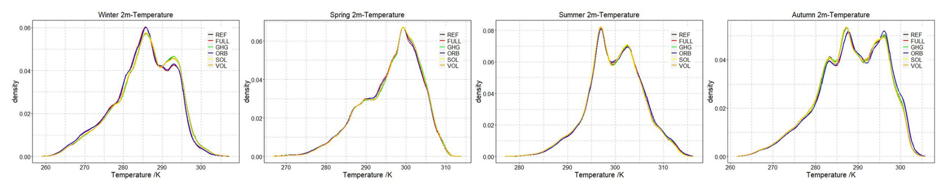
Figure 9 Density plot of the 2 m temperature for the different forcing experiments in the CCLM for each season.

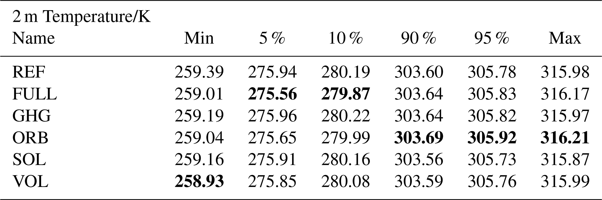
The analysis of the monthly minimum and maximum values provides insights into temperature extremes. In addition to these extremes, Table 2 shows the 5th, 10th, 90th and 95th percentiles. The lowest temperatures are simulated with the VOL followed by the FULL simulation, which presents the lowest 5th and 10th percentile values, followed by the ORB simulation. On the other hand, the highest temperatures are observed in the ORB simulation, followed by the GHG (10th percentile), and the FULL simulation (5th percentile and maximum). Overall, the FULL and ORB simulations represent the most extreme temperature values, whereas, the REF, SOL and GHG simulations reflect more moderate values.

Table 2 Minimum and maximum monthly mean temperature values across the entire domain and the whole decade of the different experiments and 5th, 10th, 90th and 95th percentiles. The experiments with the most extreme values are denoted in bold.

3.2 Precipitation

3.2.1 Comparison ESM – RCM

The general surface cooling caused by volcanic aerosols after the 1257 Samalas eruption is accompanied by various impacts on atmospheric circulation, including changes in atmospheric humidity and precipitation patterns. The reduction in surface temperatures increases atmospheric stability, leading to decreased convection and evapotranspiration. After a major volcanic eruption, this theoretically leads to lower atmospheric humidity and reduced precipitation on a global scale. On the regional scale, this pattern might be modified or even reversed because of changes in major regional circulation systems (i.e. monsoon, changes in ITCZ), whose influence on the regional climate is considerably larger. It is therefore possible that the influence of the volcanic eruption on precipitation variability will only become visible years later through secondary processes and feedback mechanisms. The higher resolved topography of the CCLM is expected to influence the spatial distribution of precipitation compared to the ESM. Figure 10 represents the monthly mean precipitation sum and standard deviation for both models. While precipitation patterns exhibit similarities, significant deviations are observed in regions with pronounced orographic gradients and/or complex coastlines, owing to the higher resolution of the CCLM. In areas temporarily influenced by the ITCZ, the CCLM shows significantly higher precipitation totals and standard deviations compared to the MPI-ESM-LR. Additionally, the CCLM effectively distinguishes between land and sea areas, as evident by higher precipitation totals along the coasts, especially over the Balkans, the Black Sea, the Caspian Sea and the Red Sea. The effect of higher resolution on precipitation is more complex than for temperature, due to smaller scale thermodynamical, hydrological and cloud microphysical processes, what is partly also connected to higher altitudes. The stark contrast between the sea-level coasts and coastal mountainous regions leads to a forced uplift of air masses, leading to condensation and subsequent precipitation. This effect is particularly notable on the luv sides of the mountains, notably along the Adriatic east coast, the east coast of the Black Sea and the eastern Red Sea, with increased precipitation.

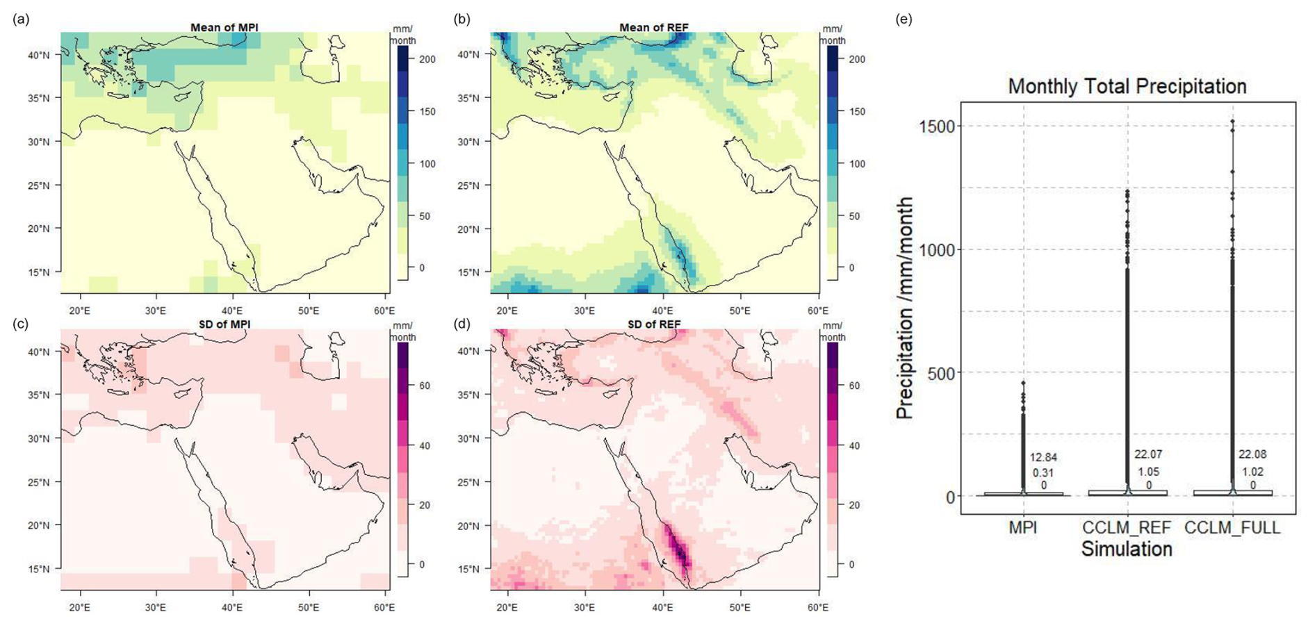
Figure 10 Mean (a, b) and Standard Deviation (c, d) of total monthly precipitation in mm/month for the period 1255 to 1264 in the driving MPI-ESM-LR (a, c) and the fully forced CCLM (b, c) and violin plot together with boxplot of the total monthly precipitation sums in mm/month of the full EMME domain and decade (e, values are upper quartile, median, lower quartile).

The right part of Fig. 10 shows the violin and box plots of the total monthly precipitation. In many regions with no precipitation, the lower quartile of monthly precipitation in both MPI-ESM-LR and CCLM simulations is zero, making the violin and box plots appear less distinct. However, differences become evident in the median and upper quartile values. In the CCLM simulations (1.05 mm/month for REF and 1.02 mm/month for FULL), the median precipitation is approximately three times higher than that in the MPI-ESM-LR (0.31 mm/month). Similarly, the upper quartile of the precipitation sum in the CCLM (22.07 mm/month for REF and 22.08 mm/month for FULL) is almost double that in the ESM (12.84 mm/month). Furthermore, outliers in the CCLM simulations reach values more than three times higher than those in the ESM simulation.

3.2.2 Annual and Seasonal Distribution

Figure 11, left, illustrates the mean monthly precipitation sum for 1255 to 1264. The CCLM simulations show clearly higher precipitation sums than the MPI-ESM-LR while also showing different shapes. In 1258, the first year after the eruption, in all CCLM simulations there was a clear decrease in precipitation compared to 1257 (the eruption occurred in September), with a reduction of up to 3 mm/month (approx. 15 %). The reduction is most pronounced in the VOL and FULL simulations. The lowest precipitation amount of the decade is observed in 1255, which predates the eruption. Conversely, the year 1260, the third year after the eruption, exhibits the highest precipitation values of the 10 years. There is no indication of a link between the volcanic or any other forcing and precipitation. The timeseries shows the natural variability of precipitation within a decade. Due to limited resources, ensemble simulations or longer timeseries were not carried out, which would have made it possible to distinguish between natural fluctuations and external forcing.

The differences between the mean monthly precipitation sums of the sensitivity simulations and REF are presented in Fig. 11, right. Before the Samalas eruption, the VOL simulation shows similar precipitation amounts to REF. However, after the eruption in 1258, the difference between the simulations reached its peak with an average reduction of about 1 mm/month in the VOL and FULL simulations. The volcanic forcing induces a decrease in precipitation due to surface cooling, resulting in increased atmospheric stability and reduced evapotranspiration. Due to the increased complexity of potentially modified general circulation patterns caused by the surface cooling, the influence of the volcanic eruption on precipitation variability becomes less dominant after one to two years. While the FULL simulation reflects the cumulative effect of the individually forced simulations, the ORB simulation demonstrates higher precipitation levels, whereas the GHG and SOL simulations show only minor differences. Again, the differences are small, especially compared to the MPI-ESM-LR, and they could have been more robust with an ensemble of simulations. However, this was not possible due to limited resources.

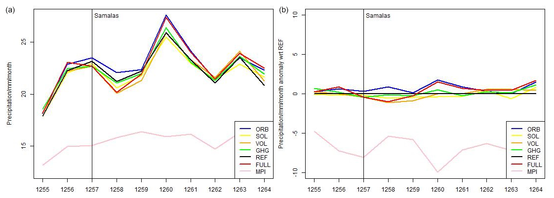
Figure 11 Annual mean total monthly precipitation in mm/month averaged over the EMME domain (a) for the CCLM simulations with the different forcings and the MPI-ESM-LR and the same values represented as anomaly (b) with respect to the reference CCLM from 1255 to 1264.

The spatial distribution of those mean values for the different years of the decade 1255 to 1264 and sensitivity simulations with respect to REF (Fig. B2 in Appendix B) present similar outcomes as Fig. 11. The differences are most pronounced in regions influenced by the tropical circulation, where mean precipitation levels are typically highest. Following the volcanic eruption, neither the FULL nor the VOL simulations reveal distinct differences compared to the REF simulation. The precipitation differences fall within the range of natural fluctuations and lack the structured temporal and spatial patterns observed in temperature, indicating no clear or strong signal attributed to an individual or combined set of forcings.

The impact of the different forcings on the seasonal mean precipitation compared to the REF simulation is depicted in Fig. 12. While most areas do not present statistically significant differences, according to the Wilcoxon-Test/Mann-Whitney-U-Test (α=0.05), most pronounced differences are observed where the total precipitation sum and standard deviation are highest (Fig. 10). Across all simulations, there is an increase in precipitation during autumn, with the largest differences observed in the FULL and ORB, especially in the southernmost parts of the domain and in Persia. These differences are related to changes in temperature due to the increased solar radiation (see Fig. 4). A similar pattern is observed in summer, albeit with more substantial differences in the southern regions. In spring, negative anomalies are small and only statistically significant here and near the Caspian Sea in the FULL simulation. In contrast, differences in winter are negligible.

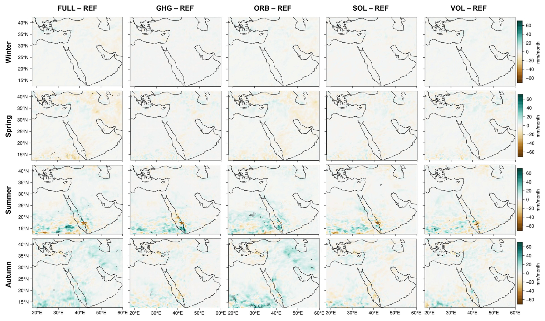
Figure 12 Seasonal mean of monthly precipitation sums for the decade 1255–1264 for the different simulations compared to REF in mm/month. Significant differences are marked with a dot (Wilcoxon-test, α=0.05). From left to right – FULL, GHG, ORB, SOL, VOL and from top to bottom – winter, spring, summer, autumn.

In summary, the annual and seasonal distribution of precipitation appears to be less influenced by external forcing compared to the 2 m temperature. This is connected to the intricate processes involved in precipitation generation, especially on local to regional spatial scales. It is likely that an ensemble of different global ESM simulations could identify varying years with the lowest precipitation during the simulated decade, regardless of changes in external forcing. Following the volcanic eruption, a slight reduction in precipitation is observed, with more pronounced impacts in simulations that include volcanic forcing (VOL, FULL). Seasonality is also only minimally affected, with a slight increase in precipitation in the southern part of the domain during summer and autumn, a trend that is somewhat more pronounced in simulations with orbital forcing (ORB, FULL). This could be connected to the ITCZ, with its most northern position during northern hemispheric summer.

3.2.3 Monthly Totals – Distribution and Extremes

In this section, we explore the distribution of total monthly precipitation values for different simulations in each grid box and month in the EMME domain over the decade encompassing the Samalas eruption (Fig. 13). The lower quartile of total monthly precipitation is zero in all simulations, reflecting locations with no precipitation throughout the year. The differences in the median range from 0.9 (SOL) to 1.05 mm/month (REF), while the upper quartile values span from 21.37 (SOL) to 22.56 mm/month (ORB), showing minor variations. Outliers vary strongly, with maximum values ranging between 1200 and 1500 mm/month. The FULL simulation records the highest value, while the ORB and GHG simulations demonstrate a high density of very high values.

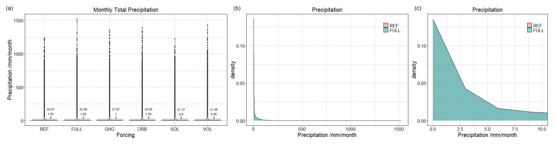
Figure 13 Violin plot combined with boxplot (a, values are upper quartile, median, lower quartile) of the precipitation for the different sensitivity experiments and density plot (c) of the monthly total precipitation in mm/month for the REF and the FULL CCLM simulation. (c) is the same as the center but showing a limited × value range.

Density plots depicting the monthly total precipitation in the REF (red) and FULL (turquoise) CCLM simulations are shown in the center and right parts of Fig. 13. However, due to the broad range of monthly precipitation, distinguishing the difference becomes challenging in the plot covering the entire spectrum (center part of Fig. 13). Therefore, the x-axis values are constrained to 10 mm/month in the right part of Fig. 13 to facilitate comparison. Given the similar distributions in both simulations, the seasonal scale (again with an x-axis limited to 10 mm/month) is presented in Fig. 14. In summer, the VOL and SOL simulations exhibit a higher density of zero and low monthly precipitation totals compared to the REF and GHG simulations, while the ORB and FULL simulations demonstrate the lowest density. Equally, in the other seasons, the distributions remain similar across all simulations. In general, spring shows the highest density of zero precipitation, followed by summer, fall and winter. A moderate monthly precipitation total of 2.5 mm/month displays the highest density in summer, followed by fall and winter, with the lowest density observed in spring. A precipitation sum of 5 mm/month is most frequent in summer, with small differences noted between the other seasons.

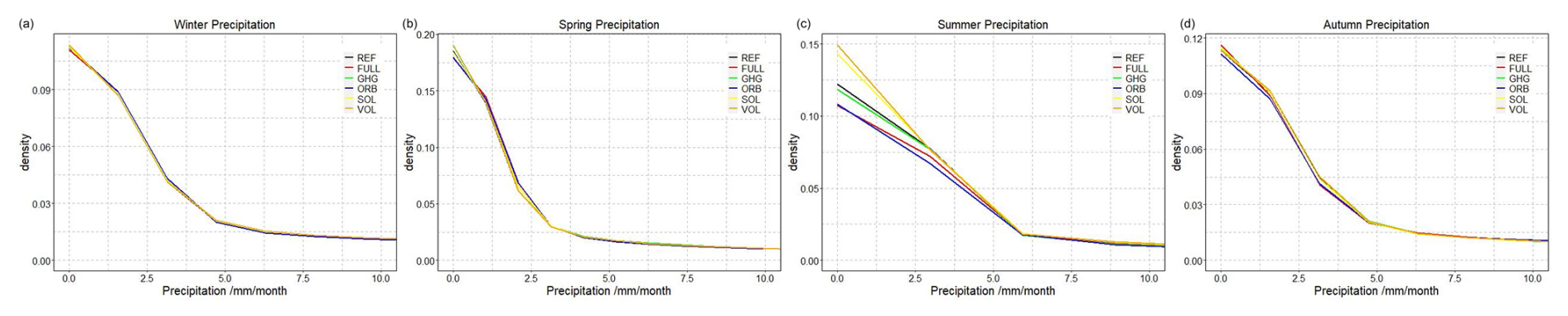
Figure 14 Density plot of the monthly precipitation (only shown up to 10 mm/month) for the different forcings in the CCLM and for every season.

The spatial distribution of minimum and maximum values for all simulations compared to REF is shown in Fig. C2 in Appendix C. Given that minimum precipitation is expected to be zero across most regions and in all simulations, the differences compared to the REF are consequently very small. Similarly, the differences in the maximum monthly precipitation totals, reaching up to 1500 mm/month, are also much greater, which is particularly evident in summer and fall, especially in the subtropical and tropical regions partly affected by the ITCZ in the northern hemispheric summer. However, no clear anomaly signal is evident, indicating that these differences are not attributable to physical processes triggered by changes in external forcings.

Table 3 shows the 50th, 75th, 90th, 95th and 99th percentiles and maximum values of the monthly precipitation totals. The 50th, 75th, 90th and 95th percentiles are highest for ORB simulation, while the highest 99th percentile and maximum values are observed in the FULL simulation. Generally, the FULL and ORB simulations capture the highest precipitation values, while the REF, GHG, SOL and VOL simulations reflect more moderate values. Additionally, the FULL and VOL simulations show the highest maxima.

Table 3 50th, 75th, 90th, 95th and 99th percentiles and maximum total monthly precipitation values in mm/month across the full area and the whole decade of the different experiments. The experiment with the most extreme value is in bold.

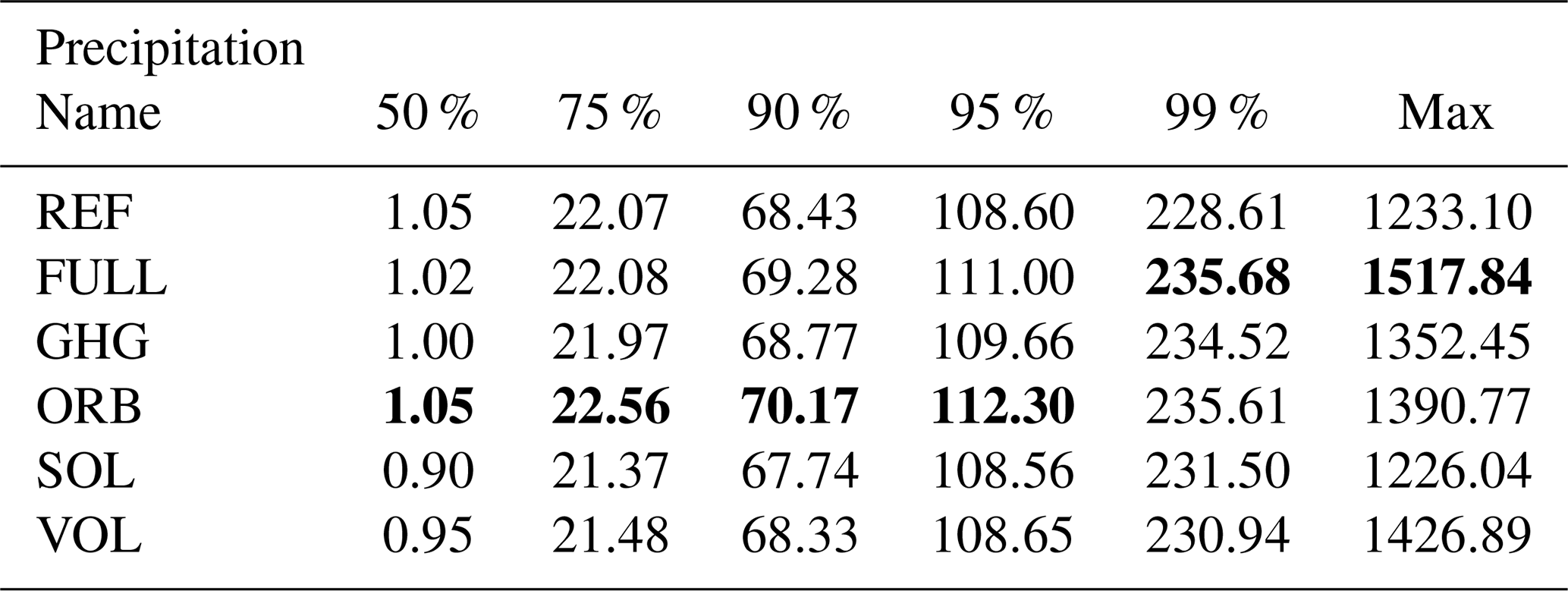
In summary, the FULL simulation produces the largest monthly precipitation sums among the test simulations. However, these are considered outliers, and thus, the statement cannot be generalized. Nevertheless, since the 90th and 95th percentiles are also highest in the simulations with orbital forcing (ORB, FULL), it suggests that overall the monthly precipitation totals can reach higher values. When looking at the seasonal precipitation totals, the differences between the simulations are most pronounced in summer.

4 Conclusions and Outlook

In this study, we implemented external climate forcings into the regional climate model COSMO-CLM to assess their individual impacts on regional climate, focusing on a substantial volcanic event, the Samalas eruption in 1257. We conducted simulations spanning ten years using various configurations: the original CCLM setup (REF), each forcing implemented separately, which are greenhouse gases (GHG), orbital (ORB), solar (SOL), and volcanic (VOL) forcing, and a fully forced model (FULL). While solar and greenhouse gas forcings played minor roles due to their limited variability within the chosen period, volcanic forcing had a significant impact, particularly in response to the Samalas eruption. Due to limited resources, an ensemble of simulations or a longer timeseries could not be carried out for each forcing. These steps will be taken in future publications, which will focus on the climate variability of specific time periods. The current study focuses purely on the influence of the different forcings, which is evident in individual simulations.

Direct implementation of volcanic forcing led to an additional cooling effect after the eruption in the test simulations. Thus, the simulations support the literature cited in the introduction, showing particularly low temperatures in 1258 and 1259 across the entire domain. However, in general, we do not analyze the eruption's absolute effect, but rather focus on the differences resulting from the implementation of each of the forcings compared to a reference without explicit forcings. The standard CCLM (reference simulation) is calibrated to the present state, thereby accentuating the linear time-dependent orbital influence. The orbital forcing influenced the timing and intensity of the seasons by changing the position of the Earth in relation to the sun on longer time scales in the order of centuries. During the Samalas period, there were slight changes in seasonality compared to the present-day configuration in REF. Our findings indicate that reduced insolation led to lower temperatures in winter and spring, while increased insolation caused a rise in temperatures during autumn. Land-use changes and in particular the choice of external data set have a substantial impact on simulation outcomes. Because the focus of the manuscript was on the the Samalas volcanic eruption those effects were not discussed in greater detail. For consistency, we used the original external data created with EXTPAR in this analysis, but for future simulations, we intend to incorporate land-use information from the driving MPI-ESM-LR.

By incorporating external forcings, including solar, orbital, volcanic, greenhouse gas, and land-use changes, we facilitate a more detailed and high-resolution analysis of past regional climatic changes while ensuring that these critical factors are fully accounted for. In general, the implementation of forcings in the RCM appears to be of secondary importance compared to the benefits of higher resolution. However, for certain variables and their temporal and spatial variability, it might be important to correctly include forcings in the RCM. The simulated 2 m temperature strongly connects with elevation, while precipitation patterns are influenced by topography and coastlines. Both are better represented in the RCM compared to the ESM, resulting in cooler mean temperatures and higher total precipitation amounts in respective regions.

The implementation of external climate forcings presented here will serve as the foundation for an unprecedented 2500-year transient RCM simulation focusing on the Eastern Mediterranean/Middle East region. Once completed, this extensive transient simulation will be subject to further analysis in future studies with various regional, temporal and thematic focuses. Through the comparison of model outputs with paleo and proxy reconstructions, we will enhance our understanding of the impacts of individual and combined forcings on regional climate, extreme events, and the underlying processes and dynamics. Moreover, the unique new data set, generated through the implementations presented in this study, in conjunction with proxy reconstructions and historical sources for the area, will facilitate a more comprehensive understanding of potential climate-society interactions and study potential causation. This interdisciplinary approach will shed light on how past climate variations may have influenced societal dynamics, adaptation strategies, and vulnerability to environmental changes.

The method presented in this work can be adapted to any period of the past for which external forcing reconstructions are available. However, it is important to note that the significance of different forcings may vary widely depending on the chosen period. This flexibility enables researchers to explore climatic changes and their impacts across different historical contexts, contributing to a more nuanced understanding of the Earth's past climate dynamics.

Appendix A: Land-Use Change Forcing

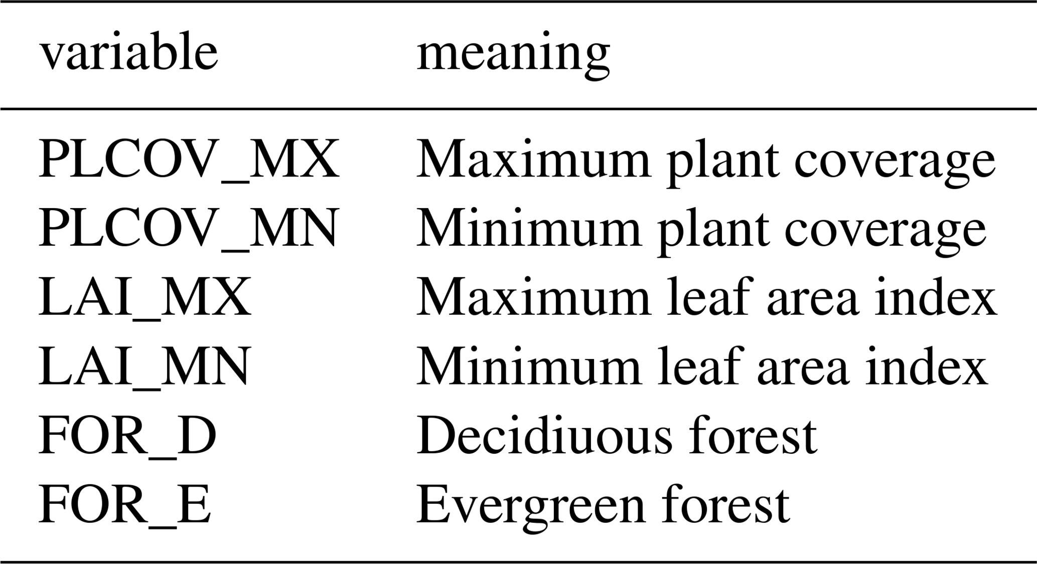
The land surface and land-use is set to a constant map in present-day studies. To implement a transient change of the land-use, the MPI-ESM-LR output is used to produce one of these maps for each simulated year. The variables needed for the land-use in CCLM are shown in Table A1. The plant coverage (PLCOV) and the leaf area index (LAI) are directly calculated with the help of the MPI-ESM-LR output variables var31 (PLCOV) and var107 (LAI). The variable for PLCOV contains ten different land cover types (tropical broadleaved evergreen and decidiuous forest, temperate/boreal evergreen and deciduous forest, raingreen and cold shrubs, C3 and C4 perennial grass, crops and pasture). The variable FOR_D and FOR_E needed for CCLM are calculated with the forest types, meaning that FOR_D is the sum of tropical broadleaved and temperate/boreal deciduous forest and FOR_E is the sum of tropical broadleaved and temperate/boreal evergreen forest. The six land-use variables are used to create an external data file for each year which is then used by the CCLM to have the information about the land-coverage.

Table A1 Land-use variables in external data created for CCLM.

Compared to the other forcings, the land-use data appears to cause a larger order of difference on the climate variables. This is because the land-surface information of the external data generated by EXTPAR and the data based on the output of the transient ESM simulation are very different. In the transient simulation the information comes periodically (e.g. yearly) from the land-model JSBACH of the driving model MPI-ESM-LR. To be used by the CCLM the JSBACH output needs to be converted to a specific format, for example by correcting the horizontal resolution. This is done for the variables LAI, PLCOV, FOR_E and FOR_D where e.g. the plant coverage is a general variable for how much of the ground is covered by plants. This is shown in Fig. A1 for the JSBACH output (topleft), the converted climatology (bottomleft) and the EXTPAR data (bottomright). The JSBACH data is divided into different land cover types. Figure A1 shows in the topright the dominant land cover type for each grid cell. In most grid cells there are also other land cover types existent but not shown here. The topleft of Fig. A1 shows the sum of all those types for each grid cell and the bottomleft shows the same but interpolated to the EXTPAR grid with a bilinear interpolation to the higher resolved grid.

In the desert regions the differences between the EXTPAR and the Climatology plant coverage are most prominent. Here are mostly growing raingreen shrubs with not very high plant coverage and C3 and C4 grass with higher plant coverage. The water and CO₂ efficient C4 grass leads to a relatively high plant coverage also in regions known as desert. In JSBACH the different land cover types are treated differently also in their effect on the atmosphere. In CCLM plants except for deciduous and evergreen forest are treated all the same with a seasonal phenological cycle.

To adequately represent the effect of the different forcings without being affected by the external influences, and to warrant a better basis for comparison, we only compare simulations with the same external surface data generated by EXTPAR.

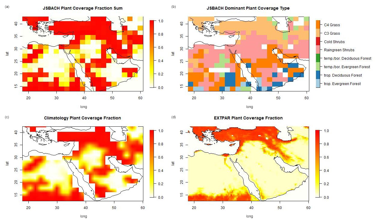
Figure A1 Distribution of the plant coverage in the JSBACH output (a) for the 1250s as interpolated for the CCLM input (c) and as given in the EXTPAR external data created for the present. The dominant land cover type for each grid cell in the JSBACH output is in (b).

Appendix B: Annual distribution maps

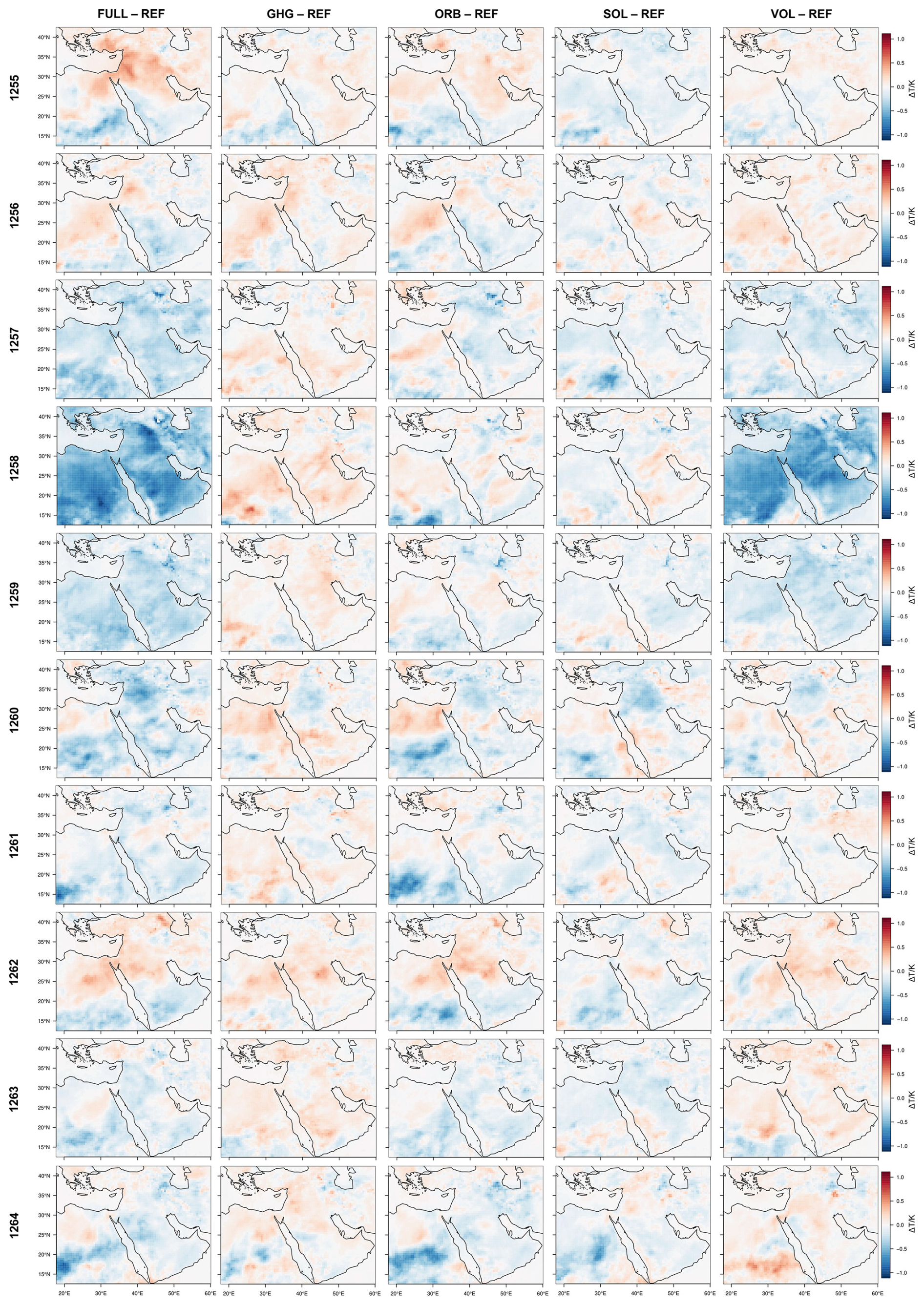
Figure B1 2 m temperature yearly distribution of differences between the differently forced CCLM simulations and the reference simulation without explicit forcing. From left to right – FULL, GHG, ORB, SOL, VOL and from top to bottom – 1255 to 1264.

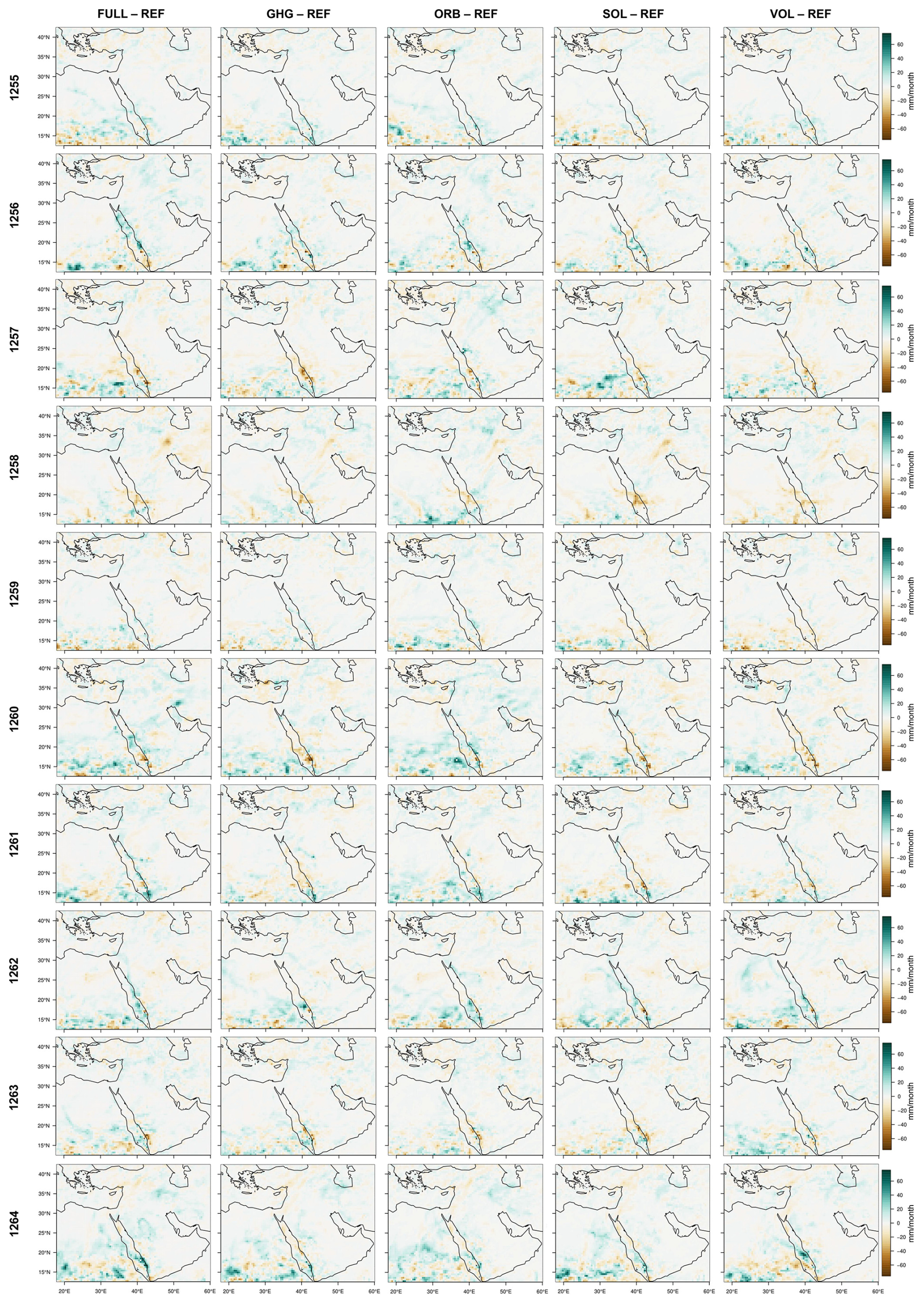
Figure B2 Yearly mean of daily precipitation anomaly for the differently forced CCLM simulations with respect to the reference simulation without explicit forcing. From left to right – FULL, GHG, ORB, SOL, VOL and from top to bottom – 1255 to 1264.

Appendix C: Seasonal minimum and maximum distribution maps

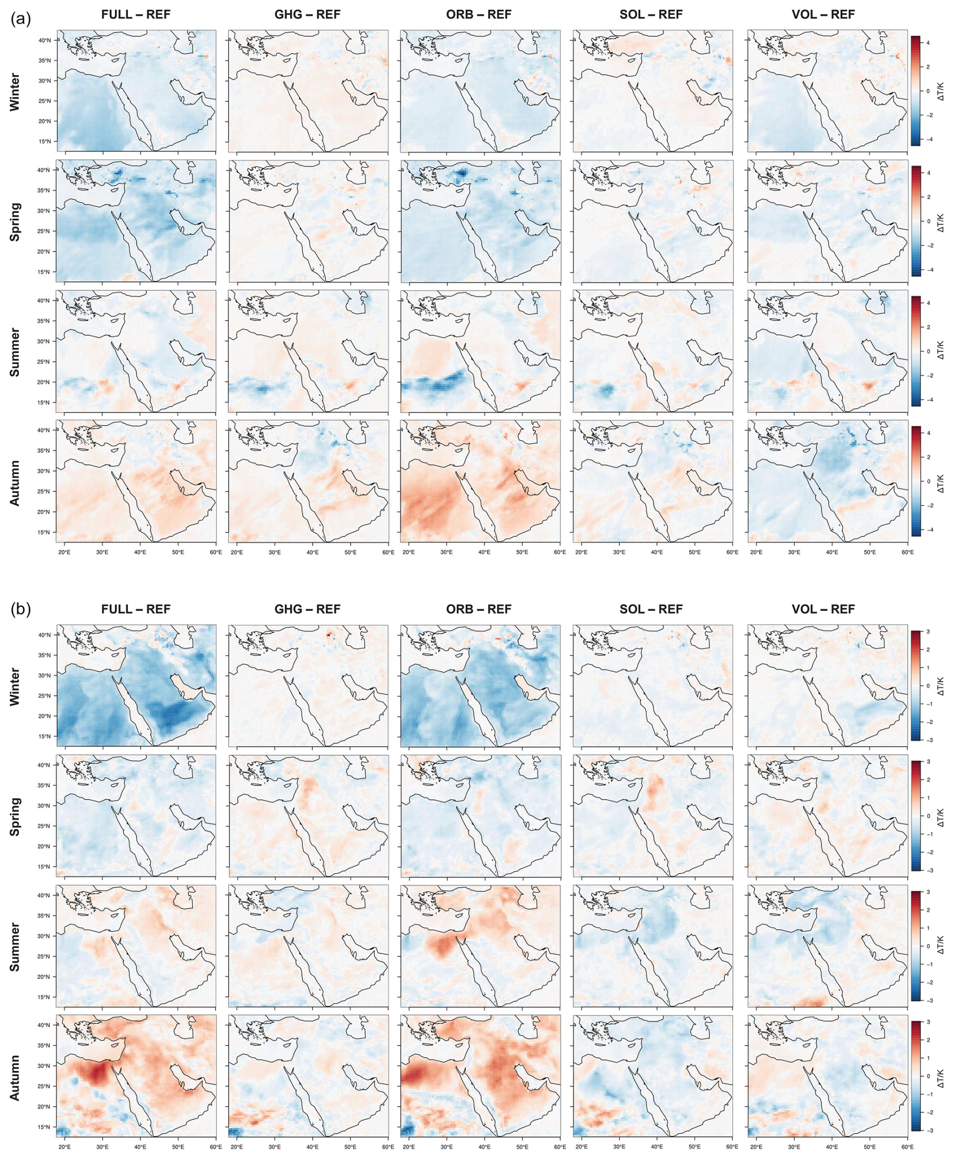
Figure C1 Seasonal minimum (a) and maximum (b) 2 m temperature distribution for the different simulations with respect to REF. From left to right – FULL, GHG, ORB, SOL, VOL and from top to bottom – winter, spring, summer, autumn.

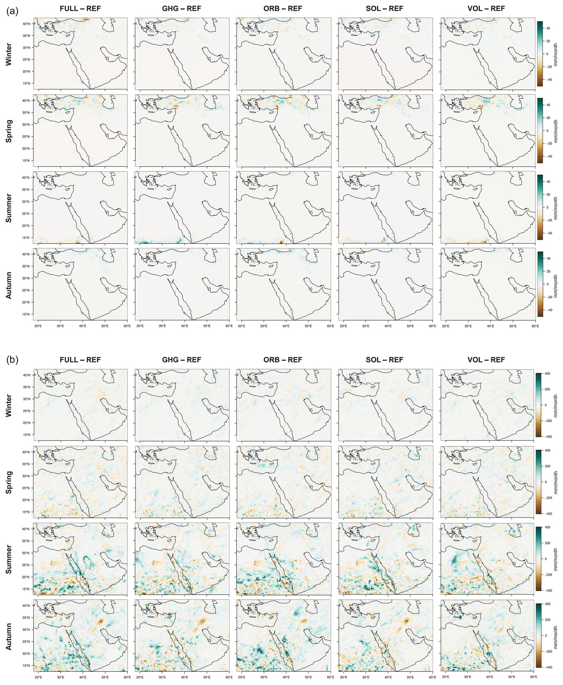
Figure C2 Seasonal minimum (a) and maximum (b) (monthly) precipitation distribution for the different simulations with respect to REF. From left to right – FULL, GHG, ORB, SOL, VOL and from top to bottom – winter, spring, summer, autumn.