Estimating biases during detection of leads and lags between climate elements across Dansgaard–Oeschger events

Dansgaard–Oeschger (DO) events occurred throughout the last glacial period. Greenland ice cores show a rapid warming during each stadial to interstadial transition, alongside an abrupt loss of sea ice and a major reorganisation of the atmospheric circulation. Other records also indicate simultaneous abrupt changes to the oceanic circulation. Recently, an advanced Bayesian ramp-fitting method has been developed and used to investigate time lags between transitions in these different climate elements with a view to determining the relative order of these changes. Here, we critically review this method in both its original implementation and a new, extended implementation. Using ice core data, climate model output, and carefully synthesised data representing DO events, we demonstrate that both implementations of the method suffer from biases of up to 15 years. These biases mean that the method will tend to yield transition onsets that are too early. Further investigation of DO warming event records in climate models and ice core data reveals that the biases are on the same order of magnitude as potential timing differences between the abrupt transitions of different climate elements. Additionally, we find that higher-resolution records would not reduce these biases. We conclude that decadal-scale leads and lags between climate elements across DO events cannot be reliably detected, as we cannot exclude the possibility that they result solely from the biases we present here.

1 Introduction

Proxy records from Greenland ice cores provide evidence of millennial-scale climate variability throughout the last glacial period (Dansgaard et al., 1982; Johnsen et al., 1992; Dansgaard et al., 1993; NGRIP members, 2004). The most striking feature of this variability is the repeated occurrence of Dansgaard–Oeschger (DO) warming events, during which Greenland temperatures increased by up to 15 K in just a few decades (Steffensen et al., 2008; Kindler et al., 2014; Capron et al., 2021) as Greenland rapidly transitioned from a cold stadial to a warm interstadial state. Alongside this rapid warming in Greenland, there is evidence of abrupt retreat of sea ice in the North Atlantic and Nordic seas (Li et al., 2005, 2010; Dokken et al., 2013; Hoff et al., 2016; Sime et al., 2019; Maffezzoli et al., 2019; Sadatzki et al., 2020) and a reinvigoration of the Atlantic Meridional Overturning Circulation (AMOC) from a rather weak stadial to strong interstadial state (Gottschalk et al., 2015; Henry et al., 2016; Lynch-Stieglitz, 2017). Furthermore, beyond the North Atlantic, a number of palaeoclimate archives provide evidence of global-scale reorganisations of the atmospheric circulation (Markle et al., 2017; Schüpbach et al., 2018; Buizert et al., 2018; Erhardt et al., 2019), including a northward displacement of the Inter-Tropical Convergence Zone (ITCZ) (Schneider et al., 2014) and changes in global precipitation patterns (Fohlmeister et al., 2023). The latter are particularly well documented in the Asian (Wang et al., 2001, 2008; Li et al., 2017) and South American monsoon regions (Wang et al., 2004; Kanner et al., 2012; Cheng et al., 2013), as well as the European–Mediterranean region (Drysdale et al., 2007; Fleitmann et al., 2009; Moseley et al., 2014; Corrick et al., 2020). However, as of yet, it has not been possible to conclusively identify a trigger for these rapid Dansgaard–Oeschger warming events (Capron et al., 2021). These periods of abrupt warming in the North Atlantic can be considered to be but one of four parts in a larger DO cycle (Lohmann and Ditlevsen, 2019). Consistent with previous studies (Erhardt et al., 2019; Riechers and Boers, 2021), we do not consider the whole cycle but only the various abrupt changes that occurred during the stadial to interstadial transitions. Henceforth, we refer collectively to these abrupt changes simply as DO events.

One paradigm in which we can consider DO events is as cascades of sudden changes in different climate variables. From this perspective, an analysis of the temporal order of events, in models or in the palaeoclimate record, should unravel the mechanistic dynamics of DO events. It is, however, important to note that such an approach relies on the assumption that all DO events are realisations of the same underlying mechanism, which may not be the case. Previous research has attempted to identify temporal lags between the sudden changes in different proxies by analysing multi-tracer records from Greenland (Steffensen et al., 2008; Erhardt et al., 2019; Capron et al., 2021; Riechers and Boers, 2021). This has the advantage that jointly measured proxy variables usually reflect the state of different components of the climate system free of any relative dating uncertainty. Nonetheless, such analysis is still difficult due to the challenge of inferring transition times from noisy data.

A Bayesian ramp-fitting method, designed to address this challenge, has been developed and presented by Erhardt et al. (2019). Stacking multiple DO events in a multi-proxy analysis of Greenland ice core data, Erhardt et al. (2019) identified time lags between the different proxies. Considering DO events back to 60 000 years before present, the authors concluded that atmospheric changes preceded the reduction in sea ice extent by around a decade. Using the same method, Capron et al. (2021) followed up on this research by extending a similar multi-proxy analysis of Greenland ice core data back to 120 000 years ago. Unlike the previous study, Capron et al. (2021) suggested that any leads and lags between climate elements might be impossible to detect due to both the tight coupling of the different climate elements and the substantial variability between different DO events.

Subsequently, Riechers and Boers (2021) re-examined the same ice core data considered by Erhardt et al. (2019), using the same ramp-fitting method but adopting a different statistical framework that more rigorously propagates the uncertainties in the onset time of each DO event. Under this new framework, the authors found that the time lags between proxies are not statistically significant, in disagreement with Erhardt et al. (2019). Therefore, although the method developed by Erhardt et al. (2019) holds much promise, it has not yet led to a conclusive understanding of the temporal phasing of DO events. Nonetheless, previous research in this area has left open the possibility that such an understanding could be achieved in future through the application of this method to either improved ice core records or data from model simulations.

Intriguingly, thanks to advances in both model development and computing power, spontaneous DO-like millennial variability is now captured by least six general circulation models (GCMs) (Brown and Galbraith, 2016; Vettoretti and Peltier, 2016; Klockmann et al., 2020; Zhang et al., 2021; Kuniyoshi et al., 2022; Malmierca-Vallet et al., 2023). The millennial variability is spontaneous in the sense that it is not externally forced by changes to atmospheric carbon dioxide concentrations or orbital parameters or by freshwater hosing. While these model simulations are imperfect representations of real DO events, they nonetheless provide an invaluable means to help us investigate the question of whether it is possible to conclusively identify a trigger for rapid Dansgaard–Oeschger warming events. We can therefore use such model simulations to test the feasibility of determining the trigger and order of changes during DO-like warming events.

We build upon these recent advances, examining in detail the causes of uncertainty in the onset time of DO events in different palaeoclimate proxies and model variables. This also enables us to comment on whether it may be possible to determine the order of changes within a DO cascade. Our paper first extends and critically reviews the Bayesian ramp-fitting method provided by Erhardt et al. (2019), investigating whether the method is biased depending on the characteristics of a given transition, as well as possible approaches to bias correction for application to real-world data. Second, we apply this method to data from the CCSM4 model (Vettoretti et al., 2022), which is chosen because the CCSM4-simulated DO events closely match real DO events in terms of their magnitude of Greenland warming, the duration of stadial and interstadial periods, and the bipolar seesaw relationship between Greenland and Antarctica. Third, we revisit the original Greenland multi-proxy data from ice cores and comprehensively investigate relevant biases. Finally, we discuss the implications of our findings for whether the temporal phasing of DO events can be determined from palaeo-data.

2 Data and methodology

2.1 Model data

The Spontaneous Dansgaard–Oeschger type Oscillations in climate models (SDOO) project, under the EU Tipping Points in the Earth System (TiPES) programme, gathers together available simulation output from models which show DO-like oscillations (https://www.bas.ac.uk/project/sdoo/#data, last access: 30 October 2024; Malmierca-Vallet et al., 2023). Included in this data set is the decadal mean output from six CCSM4 model runs which Vettoretti et al. (2022) have provided. Each of these six simulations is 8000 years long and exhibits millennial-scale variability which strongly resembles DO events, as observed in palaeoclimate archives. The runs are forced using Last Glacial Maximum boundary conditions (Vettoretti et al., 2022) alongside varying concentrations of atmospheric carbon dioxide (from 185 to 230 ppm). This range closely matches the atmospheric carbon dioxide concentrations during Marine Isotope Stage 3, when DO events were most frequent (Vettoretti et al., 2022). The number of events in each simulation depends on the CO₂ concentration, with the highest DO frequency at 200 ppm (Vettoretti et al., 2022). In total, there are 19 abrupt warming events in these six simulations.

We select five variables from CCSM4 in order to compare the timing of their relative transitions. These are North Atlantic surface air temperature, precipitation, and sea ice extent, as well as the North Atlantic Oscillation (NAO) and the Atlantic Meridional Overturning Circulation (AMOC). The first four of these are chosen as they have previously (Capron et al., 2021) been used in a similar analysis of earlier simulations from the same model, though we consider a different region. We add the AMOC to this selection due to the integral part it is thought to play in DO events (e.g. Lynch-Stieglitz, 2017; Li and Born, 2019; Malmierca-Vallet et al., 2023). We calculate time series for temperature, precipitation, and sea ice by taking area-weighted means over a selected region of the North Atlantic (shown in Fig. 4). AMOC is given by the spatial maximum of the stream function in the North Atlantic between 20 and 60° N at any depth. The NAO index is calculated as the first principal component of sea level pressure across the region 30–80° N and 80° W to 40° E.

From the resulting time series, we visually identify the abrupt warming events. For the analysis, we isolate the individual events in data windows of 800 years approximately centred on the transition. To ensure consistency, these same search windows are used for all five variables of interest.

Alongside the full data set that is available at a 10-year resolution, there are a small number of annually resolved simulations. Although we do not have a sufficient number of annually resolved abrupt warming events to assess potential systematic time lags, an application of the Bayesian ramp fit allows us to gain a sense of the ranges of the ramp and noise parameters. This in turn allows us to gain insight into how an increased resolution impacts the bias in the ramp-fitting method.

2.2 Ice core data

Alongside the model data, we also revisit data from the North Greenland Ice Core Project (NGRIP) (NGRIP members, 2004) that were previously analysed using this method (Erhardt et al., 2019). We make use of the data provided by Erhardt et al. (2019) for four proxies from this core over 16 stadial–interstadial transitions ranging in time from the Holocene onset to the onset of Greenland Interstadial 17.2 at around 60 000 years before present. While Erhardt et al. (2019) considered a larger set of transitions, these 16 are the only ones for which they were successfully able to apply their method to all four proxies.

The four proxies in this data set are δ¹⁸O, annual layer thickness, concentration of dust aerosol (Ca²⁺ ions), and concentration of sea salt aerosol (Na⁺ ions). For δ¹⁸O, the temporal resolution decreases from 4 years at the Holocene onset to 7 years at 60 000 years before present, while for the other three proxies this resolution decreases from 1 to 3 years over the same period. These four proxies have previously been interpreted as representing the air temperature at the core site, precipitation at the site, large-scale Northern Hemisphere atmospheric circulation, and sea ice extent in the oceans around Greenland (Erhardt et al., 2019). Our focus in this work is on the ramp-fitting method itself rather than a detailed consideration of the ice core proxies that we are applying it to, and so we do not make any link between particular ice core proxies and particular model output variables.

2.3 Ramp-fitting method

The Bayesian method developed by Erhardt et al. (2019), and previously applied to DO events recorded in ice cores and speleothems (Adolphi et al., 2018; Erhardt et al., 2019; Capron et al., 2021), models each event as the sum of a deterministic linear transition (or ramp) between two fixed equilibria and an additive AR(1) noise process as follows:

$$\begin{array}{}\text{(1)}& {\displaystyle }& {\displaystyle }{x}_i\left(t_i\right)={\widehat{x}}_i\left(t_i\right)+{\mathit{ϵ}}_i,\text{(2)}& {\displaystyle }& {\displaystyle }{\widehat{x}}_i\left(t_i\right)=\left\{\begin{array}{ll}{x}_{\mathrm{0}}& \mathrm{for}{t}_i\le t_{\mathrm{0}}\\ x_{\mathrm{0}}+\frac{x_{\mathrm{1}}-x_{\mathrm{0}}}{t_{\mathrm{1}}-t_{\mathrm{0}}}\left(t_i-t_{\mathrm{0}}\right)& \mathrm{for}{t}_{\mathrm{0}}<t_i<t_{\mathrm{1}}\\ x_{\mathrm{1}}& \mathrm{for}{t}_i\ge t_{\mathrm{1}}.\end{array}\right..\end{array}$$

The addition of the AR(1) noise process ϵ_i makes the model stochastic. For a given time series that comprises a DO event, the introduction of appropriate prior distributions directly yields Bayesian posterior distributions for the model parameters t₀, t₁, x₀, x₁, α, and σ, where α and σ define the autocorrelation and the amplitude of the noise. The meanings of each of these parameters, their prior probability distributions, and a full description of the AR(1) noise model are given in Appendix A.

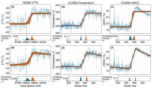
Figure 1 A comparison of the output when applying both the original (flat) implementation of the method (a–c) and the extended (slope) implementation (d–f) to three different transitions. The time series are shown in blue, with the median deterministic ramp as estimated by the Bayesian method in black and the 5 %–95 % range in orange shading. Below, the posterior distributions for the onset time and end time of the rapid transition are shown as blue and orange histograms, respectively. In panels (a) and (d), the two different implementations of the ramp-fitting method are applied to δ¹⁸O from the NGRIP core (Erhardt et al., 2019), covering the transition to GI-12c. Panels (b) and (e) show surface air temperature at the nearest grid cell to the NGRIP site across a transition from CCSM4 (Vettoretti et al., 2022), while panels (c) and (f) show AMOC for this same transition. The addition of slopes before and after the transition yields a clear improvement of the visual fit of the deterministic ramp to the CCSM4 data in panels (e) and (f), compared to panels (b) and (c).

We observe that both the model and ice core datasets contain some abrupt transitions with gradual trends before or after the transition itself (Fig. A1). This behaviour is not captured by the original Erhardt formulation, and so we extend the method by adding possible slopes before and after the linear ramp. This leads to an improved agreement of the transition model with the analysed data (Fig. 1). This is particularly the case for AMOC in the CCSM4 model, which shows an exaggerated “saw-toothed” shape with a strong downward slope following the abrupt transition. In such cases where slopes are clearly present either before or after the transition, our extended method also leads to reduced uncertainty in the onset time t₀ and end time t₁ of the transition.

Additionally, for cases where slopes are present, our extension of the method reduces the sensitivity of the transition timing to the search window, which is otherwise one of the drawbacks of this method (Capron et al., 2021). In order to apply the ramp fit to individual transitions, one has to select a data window around that transition. There are no objective criteria for the starting point and the endpoint of these windows, other than the notion that no other transition should be included. However, changing the boundaries of the data window influences the results of the estimation. This effect is reduced if slopes before and after the transition are allowed. For example, for an arbitrarily chosen transition of AMOC in the CCSM4 model, we applied both the original and extended ramp-fitting method to the same transition using 25 different search windows and found that the standard deviation in the posterior mean onset time decreased from 16.0 years when using the original method to just 4.3 years when using the extended method (Fig. A3).

However, if no such slopes are present, then our extended method results in increased uncertainty due to the addition of two unnecessary extra parameters. A full quantitative assessment of the performance of the two different implementations of the ramp-fitting method under different conditions can be found in Appendix A. Overall, when assessed in terms of timing uncertainty, neither the original nor the extended method is obviously superior, and so we consider both throughout our analysis.

2.4 Hypothesis testing

We require a means by which to test the statistical significance of any time lags that we may discover in either the model or ice core data. Although the ramp-fitting method is Bayesian, we adopt a frequentist perspective for our statistical analysis following Riechers and Boers (2021). For our analysis of the CCSM4 model, we define time lags for the transition onset of each of the other four variables relative to the transition onset in temperature T.

$$\begin{array}{}\text{(3)}& \mathrm{\Delta }{t}^x=t_{\mathrm{0}}^x-t_{\mathrm{0}}^T\end{array}$$

A negative Δt^x thus corresponds to an earlier transition onset in variable x compared to the temperature transition onset.

We regard the Δt^x from the different simulated DO events as realisations of a repeated (identical) random experiment. This view is only meaningful if one accepts the “one-mechanism” hypothesis, which states that all DO events follow the same mechanism and that differences in their expression are exclusively due to internal climate variability. While this hypothesis may not be generally accepted for DO events in the real world, we believe that the regularity of the stadial–interstadial cycle seen in the DO simulations provides a strong argument that at least the simulated DO events are all governed by the same physics. We further emphasise that a statistical assessment in terms of hypothesis tests relies on the one-mechanism hypothesis and would be meaningless if individual DO events were caused by different physical drivers.

We conduct pairwise hypothesis tests by comparing each of the other four variables to temperature using the following hypotheses:

• H₀, where the population mean time lag of this variable relative to temperature is equal to zero.

• H₁, where the population mean time lag of this variable relative to temperature is not equal to zero.

We perform two-tailed tests as we have no prior indication as to the sign or direction of any time lags that may be present.

We conduct our analysis of the NGRIP ice core in the same manner. In this instance, we calculate time lags for the other three proxies relative to Ca²⁺ and conduct hypothesis tests as above.

$$\begin{array}{}\text{(4)}& \mathrm{\Delta }{t}^x=t_{\mathrm{0}}^x-t_{\mathrm{0}}^{{\mathrm{Ca}}^{\mathrm{2}+}}\end{array}$$

Note that the choice of reference variable/proxy is arbitrary and separate between the model and ice core datasets as we are not drawing any equivalence between particular model variables and ice core proxies.

2.5 A note on nomenclature

In this work, we are dealing with two types of randomness. The first is the uncertainty in the determination of the transition time as reflected by Bayesian posterior distributions of the t₀ parameter. Second, as stated previously, we regard any set of abrupt transitions (be it in synthetic test data, GCM data, or an ice core record) as repeated realisations of the same random experiment. The transition times of the different climate components assume the role of (correlated) random variables in this perspective.

Correspondingly, there are two types of averages that we use throughout this work. For sake of clarity, we refer to averages over Bayesian posterior distributions of parameters as “posterior averages” or “posterior means”. Means over different realisations of the random experiment (i.e. over different events or transitions) are called “event averages” or “event means”.

3 Results

3.1 Synthetic transitions

As noted in the introduction, we wish to systematically test the ramp-fitting method and investigate whether there are any biases in its estimation of transition timing. Indeed, we identify the following transition parameters (Fig. 2) as potential sources of bias: (i) noise $/$ signal ratio (ξ), (ii) autocorrelation time of the noise, (iii) Greenland stadial slope, (iv) Greenland interstadial slope, and (v) transition duration. Note that the noise $/$ signal ratio is calculated by dividing the amplitude of the AR(1) noise by the amplitude of the transition and that we normalise the slopes relative to the amplitude of the transition to allow for comparison between different variables and proxies.

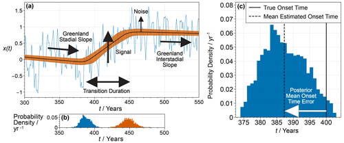
Figure 2 (a) An example of the application of our extended method to a synthetic transition with annual resolution, where the parameters of interest for the assessment of bias are marked. (b) The posterior distributions for the onset and end time of the transition. (c) An enlarged reproduction of the posterior distribution for the transition onset time with the true onset time and posterior mean estimate onset time shown. The true onset time (thick line) is set to be the year 400. The mean estimated onset time is the mean of the posterior distribution for the onset time t₀ produced by the application of the Bayesian ramp-fitting method to these noisy data. The posterior mean onset time error (PMOTE) is given by the difference between these two times, and so a negative PMOTE indicates that the transition onset has been estimated to occur earlier than it truly does.

To quantify the strength of the bias, we construct synthetic transitions by the addition of randomly generated AR(1) noise to a piecewise linear ramp, exactly as in the extended transition model (Appendix A). Our intention is not to mimic true data as realistically as possible but instead to create data to which the ramp-fitting method should be perfectly suited. We consider transitions with temporal resolutions of 10 years (decadal) and 1 year (annual) in order to investigate the impact of different resolutions on the bias. In all cases, the synthetic data series are 800 years long, with an abrupt transition that starts in the year 400. By comparing this true onset time to the posterior mean onset time as estimated by the ramp-fitting method, we calculate the posterior mean onset time error (PMOTE) for each synthetic transition (Fig. 2). Although for an individual synthetic transition the PMOTE is sensitive to the particular realisation of the AR(1) process, the event average of the PMOTE with respect to the AR(1) noise can be identified with the bias of the method. Accordingly, we take a further event mean over 100 separate synthetic transitions for each unique combination of parameter values.

Our aim is ultimately to assess the degree of bias that is propagated to estimates of leads and lags. It is not clear whether the posterior mean or posterior median onset time is more suitable to represent (or integrate) the bias, especially because two conflicting approaches have been proposed for the calculation of leads and lags from a set of events (Erhardt et al., 2019; Riechers and Boers, 2021). One would expect the posterior mean onset time to generally be somewhat earlier than the posterior median due to the asymmetry of the posterior distribution which arises because the transition duration has a lower bound at zero but no upper bound. To ensure that this does not overly affect our results, we therefore also consider the posterior median onset time in our systematic testing.

The ranges over which the parameters for the synthetic transitions are varied are chosen to reflect the ranges observed for these parameters when applying the ramp-fitting method to different events and variables in the CCSM4 model simulations, as well as different events and proxies, in the NGRIP ice core record. The appropriate ranges for the noise $/$ signal ratio (ξ) and the autocorrelation time of the AR(1) noise differ between the cases of decadal and annual resolution because higher-resolution data are generally noisier. Note that the Greenland interstadial slope is negative in all cases, reflecting the classic saw-toothed shape of DO events; however, we plot the absolute value of this slope for ease of legibility.

We would ideally like to vary all five transition parameters simultaneously in order to assess possible inter-dependencies of the bias on different transition parameters. However, it would be challenging to visualise and interpret the resulting five-dimensional parameter space. We therefore vary only two transition parameters at any one time – the noise $/$ signal ratio and one other – while keeping the rest fixed at standard values as follows:

• Autocorrelation time = 10 years for the case of decadal resolution and 1 year for the case of annual resolution.

• Greenland stadial slope = 0 kyr⁻¹.

• Greenland interstadial slope = −1 kyr⁻¹. Note that the Greenland interstadial slope is always ≤0 in our sensitivity tests, due to the saw-toothed shape of DO events. In Fig. 3, we plot the absolute value or magnitude of this slope, which is positive. Note that the slopes are normalised relative to the amplitude of the transition. This standard value for the Greenland interstadial slope therefore means that the time series will return to its pre-transition level 1000 years after the transition ends.

• Transition duration = 50 years.

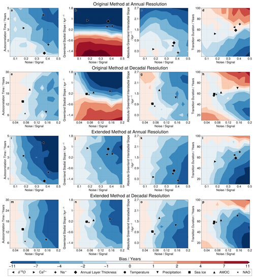
Figure 3 The bias in the posterior mean transition onset time as a function of the five transition parameters. We consider both the original (a–h) and extended (i–p) implementations of the ramp-fitting method at both annual (a–d and i–l) and decadal (e–h and m–p) resolution. Each panel contains 100 unique sets of parameter values, and for each set of parameters, we take an event average over 100 synthetic transitions. When not explicitly varied, parameters are fixed at standard values, as given in Sect. 3.1. Blue colours indicate a bias towards transition onset times that are too early, with red indicating the opposite. The mean transition parameters for the four proxies from NGRIP are overlaid in panels (a)–(d) and (i)–(l) and for the five variables of interest in the CCSM4 model in panels (e)–(h) and (m)–(p). Note that the scales for the noise $/$ signal and autocorrelation time differ between the cases of annual and decadal resolution.

Our systematic testing of the ramp-fitting method using synthetic transitions finds that the onset time estimate can be biased due to the transition parameters (Fig. 3). This is true for all four combinations of method implementation and temporal resolution considered here, but there are differences in the extent of the bias and the dependence on different parameters.

First, for the original method, we find that the Greenland stadial slope preceding the abrupt transition is the key driver of onset time bias, as shown by Fig. 3b and f. For both the NGRIP and CCSM4 events this slope is generally positive, meaning that it is in the same direction as the abrupt transition itself. We find that this leads to a bias that is too early and that can exceed 10 years, although the extremities of the range considered here (and so the largest biases) occur only rarely in the NGRIP data. We also see bias arising from variations in the other parameters but not to the same extent.

For the extended method, there is generally a bias that is too early by up to 10 years when the noise is high. We also find that the level of noise controls the strength of the impact of the other four parameters; when ξ is small, variations in the other parameters have little impact on the bias, but when this ratio is high, variations in the other parameters have a large effect (∼10 years). Focusing on the case of decadal resolution (Fig. 3h) for ξ∼0.2, an increase in the transition duration from 10 to 100 years may even reverse the bias from $\sim -\mathrm{10}$ years to $\sim +\mathrm{8}$ years. It is therefore clear that the noise $/$ signal ratio ξ is the key parameter in determining the bias of our extended ramp-fitting method but that the other parameters identified here also play an important role.

For both implementations of the ramp-fitting method, the broad pattern of bias observed is similar between the cases of annual and decadal resolution. It is not possible to say whether the bias is generally greater for one case or the other, as the transition parameters at annual resolution map onto those at decadal resolution in a complex manner. This means that points in the same positions of their respective panels in Fig. 3 are in fact not directly comparable between the two resolutions. We conduct further testing in Sect. 3.2 to explicitly address this point.

When compared to the original Erhardt et al. (2019) implementation of the ramp-fitting method, our extended implementation that includes slopes leads to a large reduction in the bias for transitions that have strong slopes before or after the transition but relatively low values of ξ. In the opposite situation, where ξ is large, and there are no slopes present, our extended implementation instead leads to increased onset time bias. Neither implementation is obviously more or less biased when considered across the whole range of possible parameter values.

The bias that we generally observe towards onset times that are too early also leads to our estimates of the transition duration being too long. This is important because the transition duration is itself one of the determining factors of the bias in the transition onset time for all four combinations of method implementation and temporal resolution (Fig. 3d, h, l, and p). Our lack of unbiased knowledge of the true transition duration therefore makes it extremely challenging to accurately estimate the bias affecting any particular model variable or ice core proxy.

Further systematic testing reveals that such bias persists, though somewhat altered, when adopting an alternative set of prior probabilities (Fig. C1) or even when taking the simplest possible approach of a least squares fit to a linear ramp (Fig. C2). This might suggest that such bias is a fundamental limitation of any attempt to identify the timing of abrupt transitions in noisy climate data. However, we equally cannot prove that there is no possible unbiased method – certainly in many other statistical settings there are estimators that remain unbiased even as their uncertainty increases. The important point for our analysis is that we do not currently possess any unbiased method that we could use to calibrate or corroborate the transition onset time or duration.

Defining the bias as the expectation of the error in the posterior median onset time, rather than the posterior mean, results in slightly more positive values for the bias (see Fig. C3), meaning that the generally negative biases we observe are somewhat decreased in magnitude. However, the differences are small and the overall pattern unchanged. This demonstrates that the choice between posterior mean and posterior median when estimating bias is unimportant, and so we only consider the posterior mean going forward.

3.2 Impact of changing resolution

We are interested in how the bias depends on the temporal resolution of the data. Although in Sect. 3.1 we have considered both annual and decadal resolution, it is far from trivial to make direct comparisons between the two. For climate time series, the changes in the noise parameters ξ and autocorrelation time when changing resolution depend on the full power spectrum of the noise. This is different for every variable or proxy and so that there is no generally applicable relationship with which to predict the impact of changing resolution. Furthermore, as previously stated, we do not have access to sufficient annually resolved data from the CCSM4 model to allow for a meaningful comparison.

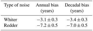
Instead, we proceed by creating two further sets of synthetic transitions at an annual resolution. These two sets of transitions represent two contrasting cases of low-autocorrelation (“whiter”) noise or high-autocorrelation (“redder”) noise, with parameters chosen based on the extremes of the range observed in the CCSM4 model. For each of these sets of synthetic transitions, we then down-sample to decadal resolution by dividing the annual time series into sections of 10 years and taking the mean over each section as a single data point for our decadal time series (Fig. C4). Finally, we separately apply our extended ramp-fitting method to the annually and decadally resolved transitions.

For both types of noise, we find that the bias is unchanged, within uncertainty, when switching between the two resolutions. These results are summarised in Table 1. We also verify that when down-sampling to decadal resolution, it does not matter whether the transition onset occurs at the edge of two averaging sections or in the middle of one. We can therefore state that the temporal resolution has no impact on the bias, although a higher resolution does at least reduce the uncertainty in the onset time estimates for individual transitions.

Table 1 The bias in the posterior mean onset time for two different types of noise at both annual and decadal resolutions in our extended ramp-fitting method each calculated from a sample of 1000 synthetic transitions. Uncertainties are given by the standard deviation of a bootstrapped distribution for the sample mean onset time error. This ensures that the uncertainties in the individual onset times are rigorously propagated.

3.3 Bias in the CCSM4 model and the NGRIP ice core record

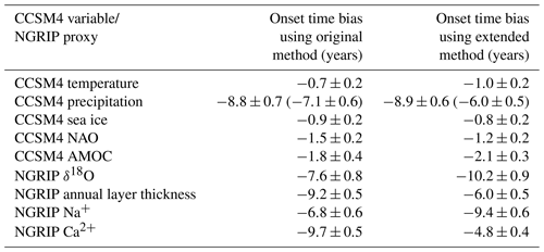
Following on from the above systematic testing, we investigate whether the ramp-fitting method introduces any bias to the timing estimation of DO events in the CCSM4 model. To do this, we construct 1000 synthetic transitions that are “analogous” to each of the model variables of interest and assess the corresponding expected PMOTE as described above. The expected PMOTE serves as a first-order approximation of the bias for each investigated climate variable and may thus be subtracted from the transition onset estimate obtained with the Bayesian ramp-fitting method. To calculate representative parameter values, we take both the posterior mean and the event mean over the corresponding marginal posterior distributions obtained by applying the extended ramp-fitting method to the 19 transitions in the CCSM4 model simulations. For each variable, this gives a single value for each transition parameter (shown in Fig. 3), which we use to create the analogous transitions.

We make an exception for transition duration, choosing instead to use a fixed duration of 50 years for all of our analogous transitions. This is because we suspect that much of the apparent difference in duration between different variables is in fact due to the bias we have identified. As we have been unable to identify any unbiased method by which to estimate the true transition durations, we simply fix them at a plausible value based on the durations of the transitions in two ice cores as estimated in a previous study (Capron et al., 2021).

The situation with precipitation is more difficult. Visual inspection of the precipitation time series reveals a much greater degree of noise during the stadials than the interstadials (Fig. C5). To test the impact of this, we investigate a further set of synthetic transitions which have two different noise regimes – one during the stadial and the other during the interstadial. We find that the value of ξ in the stadial is most important to the bias in the onset time (Fig. C6). Because of this, creating synthetic transitions using a single noise regime is likely to underestimate the magnitude of the bias affecting precipitation, and so it is important that we include these two distinct levels of noise for precipitation. To do so, we further adapt the Bayesian ramp-fitting method, producing a new version that treats noise before and after the transition separately. We find that this has a negative impact on the success rate of the Markov chain Monte Carlo (MCMC) sampler that forms part of the method in that there are many more cases where the sampler fails to converge, and so we do not attempt to use this implementation to assess the timing. Instead, it simply provides a means of calculating appropriate parameter values to use for the synthetic transitions that are analogous to precipitation.

For completeness, we construct two sets of synthetic transitions that are analogous to precipitation, namely one where we do not account for the differing noise between stadials and interstadials and one where we do. Our estimates of the magnitude of the bias are increased by around 2 years for the original method and around 3 years for the extended method when we include the two distinct noise regimes in our synthetic transitions (see Table 2). This confirms our expectation that failing to do so would lead to an underestimate of the degree of bias.

Table 2 Mean estimates and uncertainties for the biases affecting different variables in the CCSM4 model and different proxies in the NGRIP ice core, resulting from their differing noise and slope characteristics, using both the original and extended methods. Each bias is calculated as the mean of the posterior mean onset time error (PMOTE; see Fig. 2) across a sample of 1000 synthetic transitions. The uncertainties are given by the standard deviation of a bootstrapped distribution for the sample mean onset time error. These reflect the uncertainty in the bias, given a particular set of transition parameters, with the uncertainty in the timing of each individual transition rigorously propagated. There is additional uncertainty due to our imperfect knowledge of the true transition parameters that we have not attempted to quantify. The values in brackets for precipitation are the biases if we neglect the two separate noise regimes. As expected, these underestimate the true biases.

Finally, we similarly investigate potential bias in the estimated transition timing of DO events in the NGRIP ice core. Here, we follow the same procedure as outlined above for CCSM4 model data. There is, however, an additional complexity due to the differing time resolutions. For simplicity, we choose round numbers that are representative of the resolution of each proxy. We therefore use a resolution of 2 years for Ca²⁺, Na⁺, and the annual layer thickness, and a resolution of 5 years for δ¹⁸O. Where for the CCSM4 model we used 800-year sections, here we create synthetic time series that are 500 years long to match the ice core data. The true transition onset times are fixed to the year 250, and the transition durations are fixed at 50 years, for the same reason discussed with regards to the model data.

The estimated biases for both the variables in the CCSM4 model and the proxies in the NGRIP ice core, and the use of both implementations of the ramp-fitting method, are listed in Table 2. Reflecting the general pattern found in Sect. 3.1, all of the variables and proxies are negatively biased; that is, they are biased towards onset times that are too early. Importantly, the biases are different for different variables and proxies due to differences in both the ramp shapes and noise properties, and hence these biases limit our ability to assess leads and lags between associated transitions of different variables or proxies.

3.4 Time lags in the CCSM4 model in light of the bias

In the following, we compare the transition onset times of the climate variables introduced in Sect. 2.1 at DO events simulated by the CCSM4 model. In doing so, we treat all simulated DO events equivalently, irrespective of the chosen CO₂ concentration. In particular, we take into account the bias which we quantified in the previous section. For each available DO event, we apply the extended ramp-fitting method to our selection of climate variables on the predefined data window.

For sea ice, AMOC, and NAO, we observe that the transition onsets occur approximately simultaneously with those in temperature, irrespective of the bias correction (Fig. 4), and so we do not discuss the hypothesis tests for these three variables. For precipitation, the story is different. Without any bias correction, the event-averaged time lag appears to be negative with certainty. Even under consideration of the bias, the uncertainty distribution of the precipitation–temperature lag is centred at around −10 years with only small probabilities for a positive lag. This indicates that the transition onsets in precipitation are likely to occur before those in temperature. However, it is not clear whether this is statistically significant. Performing a hypothesis test, as described in Sect. 2.4, we calculate a p value of 0.078. As this is slightly greater than the standard significance threshold of 0.05, we cannot ultimately rule out the null hypothesis that the transitions in temperature and precipitation occur simultaneously. This demonstrates how the bias we have identified can lead to false conclusions about the significance or otherwise of time lags between different variables or proxies.

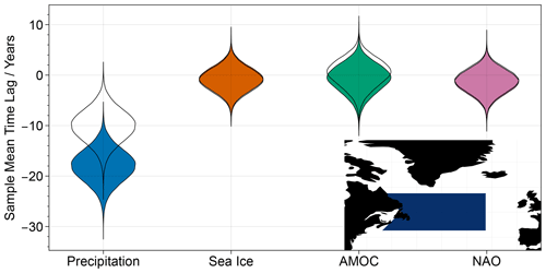
Figure 4 Uncertainty distributions for the uncorrected (filled) and bias-corrected (transparent) sample mean time lags of precipitation, sea ice, AMOC, and NAO as compared to temperature in the CCSM4 model, according to our extended ramp-fitting method. The bias correction is applied to the reference variable, temperature, and the target variable. The inset is a map showing the region of the North Atlantic over which temperature, precipitation, and sea ice have been averaged. (Vettoretti et al., 2022).

3.5 Time lags in the NGRIP ice core in light of the bias

Following the same procedure as for the model warming events, we calculate the sample mean time lags of Na⁺, δ¹⁸O, and annual layer thickness, relative to Ca²⁺, in the NGRIP ice core using our extended ramp-fitting method. We again use the analogous synthetic transitions to perform a bias correction. Note that in this case each random sample is comprised of 16 of these synthetic transitions, as this is the size of our sample of DO events in the ice core. For each of these proxies, Fig. 5 clearly shows that the bias-corrected distributions are consistent with zero time lag, and so we do not discuss the formal hypothesis tests.

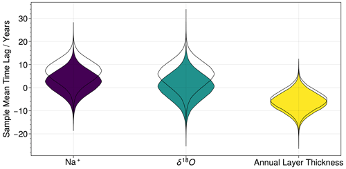
Figure 5 Probability distributions for the uncorrected (filled) and bias-corrected (transparent) sample mean time lags of Na⁺, δ¹⁸O, and annual layer thickness compared to Ca²⁺ in the NGRIP ice core (NGRIP members, 2004; Erhardt et al., 2019), according to our extended ramp-fitting method. The bias correction is applied to the reference proxy, Ca²⁺, and to the target proxy.

4 Discussion

We have demonstrated that the commonly used ramp-fitting method is biased by up to 10 years when estimating the onset time of DO events. This is comparable to the magnitude of the time lags we might expect to find between different components of the climate (Erhardt et al., 2019), and so this bias severely limits the trust that we may have in any time lags identified in this manner. We have attempted, in Sect. 3.4, to correct for this bias in order to produce a more accurate estimate of the true time lags. In doing so, we found that even a large apparent time lag, such as the 18-year time lag we observed between precipitation and temperature in the CCSM4 model, could simply be the result of methodological bias.

One important caveat is that the bias we have identified is generally fairly small relative to the timing uncertainty in individual proxies across single DO events, which is usually several decades (see, e.g., Fig. A2). Our bias of up to 10 years is therefore unlikely to critically impact the findings of studies which only consider and compare individual transitions, for example (Capron et al., 2021). However, the calculation of leads and lags may involve stacking many events so as to reduce the uncertainty – sometimes to as little as ±5 years (Erhardt et al., 2019). In this context, the bias that we have identified is clearly extremely important to consider, as it could easily lead to false conclusions, as we saw for the model data in Sect. 3.4.

Capron et al. (2021) also test for possible bias using synthetic transitions with autocorrelated noise and find no significant bias in either the transition midpoint or duration, implying that the transition onset time must also be unbiased. This stands in contrast to our findings in this study and so merits further consideration. We suggest that the transitions tested by Capron et al. (2021) lie in a region of the parameter space for which the bias is small, even at high levels of noise. The most obvious reason for this is that the absence of any slopes before or after the ramp favours small biases. We observe in Fig. 3 that, when using the original Erhardt et al. (2019) implementation, synthetic transitions without any slopes before or after the ramp show very little bias, even for relatively high levels of noise. However, the bias grows rapidly when even slight slopes are present. We therefore suggest that a key cause of the discrepancy is the assumption made by Capron et al. (2021) that there are no slopes in either the stadial that precedes the transition or the interstadial that follows. Similarly, Fig. 3 shows that for certain “sweet spots” in the transition duration, the bias remains small even as the level of noise increases. It could also be the case that the transition duration chosen by Capron et al. (2021) happens to lie in such a sweet spot and that this is partly why they do not find significant bias.

In the frequentist framework that we have adopted, two key uncertainties enter into our hypothesis test for the significance of the difference in onset time between precipitation and temperature. These are the inherent uncertainty in the timing estimate of DO events and the uncertainty in the mean of a finite sample, which combine to form large uncertainties in both the observed and empirical null time lags. Considering this, the p value of 0.078, though above the standard significance threshold of 0.05, may still appear rather small. This could suggest that the potential lead of precipitation merits further investigation. However, the standard significance threshold should really be adjusted downwards to correct for the fact that we have made multiple comparisons by comparing precipitation, sea ice, AMOC, and NAO to temperature. We do not feel the need to explicitly make this correction in this case because our finding is not significant even at the uncorrected threshold, and also because it is not clear precisely how this should be done. Nonetheless, this further strengthens the view that it is not possible to make any firm conclusion regarding the temporal phasing of DO events.

This is even more so the case when we consider the major limitations of our bias correction. The first of these is that we have followed the simplest possible approach of using single values for the parameters of our synthetic transitions. It would be more appropriate to instead sample from the range of parameter values exhibited by the same variable/proxy across different DO events. However, utilising the distribution of parameters in this way leads to estimates of the bias that are so uncertain as to lose meaning, and so we have used single-parameter values (as given by combined posterior and event averages). Furthermore, the bias depends in a highly non-linear manner on interactions between the different transition parameters, and so our assumption that the bias resulting from the mean parameters is equal to the mean bias resulting from the whole range of parameters is a poor one.

Another issue limiting the possibility for bias correction is our inability to estimate the transition duration in an accurate manner. This has a major impact because the transition duration is a key determinant of the bias in the transition onset time; however, the duration itself is also affected by this bias. We are thus stuck in an impossible situation whereby we cannot know the duration without first knowing the bias, but we simultaneously cannot know the bias without first knowing the duration. Because of this, the best we are able to do is to guess a plausible transition duration; we chose 50 years in all cases. The fact that these DO transition durations also cannot be determined is another important source of uncertainty that cannot be captured by a bias correction procedure.

Given these limitations of the bias correction procedure, there are clearly additional uncertainties affecting the time lags discussed in Sect. 3.4 and 3.5 which we have not attempted to quantify. Even without incorporating these additional uncertainties, we reiterate that the identification of a statistically significant order to the DO events remains very challenging. A higher temporal resolution would allow us to somewhat reduce the uncertainty in the timing estimate of each DO event. But, as Sect. 3.2 shows, the temporal resolution of the data comprising a transition has no impact on the bias in the ramp-fitting method. There is therefore a limited prospect for improving this situation in the future through access to higher-resolution model output data or indeed higher-resolution palaeo-measurements from ice cores.

5 Conclusions

Bayesian ramp-fitting methods have shown great potential as a tool for identifying the temporal phasing of the changes in different climate components during climate transitions. For DO events, however, we demonstrate that even the advanced method of Erhardt et al. (2019) suffers from bias when estimating the onset time of these very fast transitions due to a combination of noise and the presence of gradual slopes before and after the transitions. Directly incorporating said slopes into the ramp-fitting method reduces the extent of the bias when significant slopes are in fact present in the data, but doing so also worsens the problem when they are not, as is often the case. The bias ranges from approximately −15 and +5 years and so is comparable to or longer than the potential relative phasing of the climate elements that we seek to resolve. This severely limits the reliability of any time lags regardless of whether they are in models or ice cores that are found when using this ramp-fitting method. It is difficult to ascertain the magnitude of this bias in any individual case for any DO events, and so any attempt to correct for the bias will necessarily introduce major additional uncertainty.

This leads to the conclusion that it may never be possible to confidently determine the order of Dansgaard–Oeschger warming events from these types of methods, no matter how many new ice cores are drilled or how many higher-resolution measurements are taken because neither of these would alleviate the fundamental problem of bias in the method. In this way, our work helps underpin the conclusion of Capron et al. (2021), who previously suggested that “it may be elusive to search for a single sequence of events”. The Bayesian ramp-fitting method considered in this study remains a powerful tool for investigating individual abrupt transitions, as the bias that we find is small relative to the uncertainty in individual events. When calculating leads and lags from a sample of events, however, the bias becomes large relative to the uncertainty and so is likely to lead to false conclusions. It therefore appears impossible to reliably determine the temporal phasing when dealing with decadal-scale time lags such as those that have been suggested for DO warming events. This does not necessarily exclude the careful application of this method to ascertain the phasing of different climate elements or proxies where the duration of the transition is longer (for example, DO cooling events). However, further careful research would be required into any alternative applications to longer duration climate transitions.

Appendix A: Ramp-fitting method

To test whether ice core data show significant slopes in the stadial periods preceding DO events, we consider the data segments used by Erhardt et al. (2019). We only consider data up to the fifth percentile of the posterior distribution for the transition onset time, as given by Erhardt et al. (2019), to ensure that the abrupt transition itself does not influence our results. We also only consider the 16 DO events for which Erhardt et al. (2019) provide onset times for all four proxies. We calculate linear slopes and test the significance of these using phase-randomised Fourier surrogates which preserve the autocorrelation structure of the data. We find that 7 of the 16 events show a significant slope (p<0.05) in Ca²⁺ that is in the same direction as the following abrupt transition (Fig. A1), as well as 4 for the annual layer thickness and 1 for Na⁺. This demonstrates the need to consider the impact of pre-transition slopes on the accuracy of the ramp-fitting method and to test whether this can be improved by directly incorporating said slopes into the transition model. This is in addition to the more obvious need to consider post-transition slopes due to the classic saw-toothed shape of DO events.

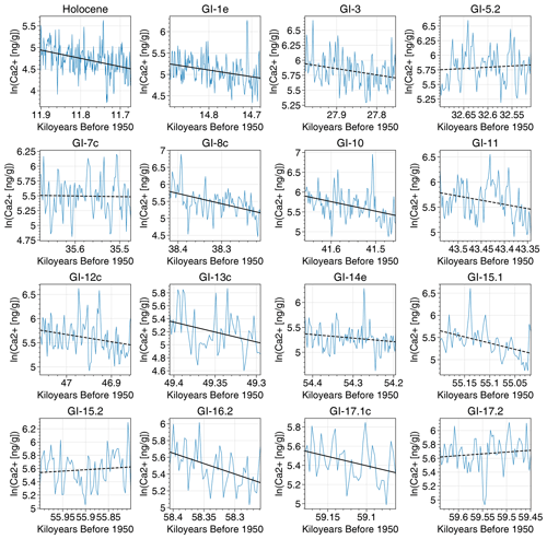
Figure A1 Slopes in the pre-transition stadial for NGRIP Ca²⁺. Solid black lines indicate statistically significant downwards slopes (p<0.05 from a one-tailed hypothesis test using phase-randomised Fourier surrogates), while dashed black lines show non-significant slopes.

The deterministic component of the transition model used by Erhardt et al. (2019) to fit a series of observations x taken at time t is as follows:

$$\begin{array}{}\text{(A1)}& {\widehat{x}}_i\left(t_i\right)=\left\{\begin{array}{ll}{x}_{\mathrm{0}}& \mathrm{for}{t}_i\le t_{\mathrm{0}}\\ x_{\mathrm{0}}+\frac{x_{\mathrm{1}}-x_{\mathrm{0}}}{t_{\mathrm{1}}-t_{\mathrm{0}}}\left(t_i-t_{\mathrm{0}}\right)& \mathrm{for}{t}_{\mathrm{0}}<t_i<t_{\mathrm{1}}\\ x_{\mathrm{1}}& \mathrm{for}{t}_i\ge t_{\mathrm{1}}\end{array}\right..\end{array}$$

The four parameters, x₀, Δx, t₀, and $\mathrm{\Delta }t=t_{\mathrm{1}}-t_{\mathrm{0}}$, are the initial value, the magnitude of the transition, the time at which the transition starts, and the duration of the transition. There are two further parameters, σ and τ, that govern the AR(1) noise which is added to the deterministic ramp in order to represent climate variability. This gives a total of six parameters. The AR(1) noise process is governed by the equations:

$$\begin{array}{}\text{(A2)}& {\displaystyle }& {\displaystyle }{\mathit{ϵ}}_{i+\mathrm{1}}={\mathit{\alpha }}_i{\mathit{ϵ}}_i+{\mathit{\sigma }}_{\mathrm{eff},i}{\mathit{\zeta }}_{i+\mathrm{1}},\text{(A3)}& {\displaystyle }& {\displaystyle }{\mathit{\sigma }}_{\mathrm{eff},i}=\mathit{\sigma }\sqrt{\mathrm{1}-{{\mathit{\alpha }}_i}^{\mathrm{2}}},\text{(A4)}& {\displaystyle }& {\displaystyle }{\mathit{\alpha }}_i=\exp \left(-{\displaystyle \frac{t_{i+\mathrm{1}}-t_i}{\mathit{\tau }}}\right),\end{array}$$

where ζ_i is a normally distributed random variable with unit variance. The variance of this AR(1) noise process is given by σ² and the autocorrelation time by τ. If the time step $t_{i+\mathrm{1}}-t_i$ is constant, then α is also constant, but we allow for the possibility of unevenly sampled data where $t_{i+\mathrm{1}}-t_i$ varies.

Given the transition model and the transition data, the Bayesian theorem can be applied to infer posterior probabilities for the model parameters as follows:

$$\begin{array}{}\text{(A5)}& p\left(\mathit{\theta }\right|\mathcal{D})={\displaystyle \frac{p\left(\mathcal{D}\right|\mathit{\theta }\left)p\right(\mathit{\theta })}{p\left(\mathcal{D}\right)}},\end{array}$$

where the probability, given the parameters θ, that the model exactly reproduces the data p(𝒟|θ) is named the likelihood. The prior distribution p(θ) of the model parameters encodes any a priori knowledge on the parameters, for example, the required positivity. The marginal probability of observing the data p(𝒟) is in this context nothing but a normalisation constant which in practice is not relevant. We somewhat alter the priors used by Erhardt et al. (2019) in order to ensure that we can apply the ramp-fitting method to different variables across a wide range of magnitudes and units. First, we calculate initial guesses for the six parameters based on simple heuristics and shift the time series such that our initial guess for the transition onset time t₀ lies at time t=0. The priors used are then as follows:

$$\begin{array}{}\text{(A6)}& {\displaystyle }& {\displaystyle }p\left(t_{\mathrm{0}}\right)=\mathcal{N}\left(\mathrm{0},{\mathrm{50}}^{\mathrm{2}}\right),\text{(A7)}& {\displaystyle }& {\displaystyle }p\left(\mathrm{\Delta }t\right)=\mathrm{Gamma}(\mathrm{2.0},\mathrm{0.02}),\text{(A8)}& {\displaystyle }& {\displaystyle }p\left(x_{\mathrm{0}}\right)=\mathrm{1},\text{(A9)}& {\displaystyle }& {\displaystyle }p\left(\mathrm{\Delta }x\right)=\mathrm{1}\text{(A10)}& {\displaystyle }& {\displaystyle }p\left(\mathit{\sigma }\right)=\mathrm{1}\mathrm{for}\mathrm{0}<\mathit{\sigma }\le \left|\mathrm{\Delta }y\right|,\text{(A11)}& {\displaystyle }& {\displaystyle }p\left(\mathit{\tau }\right)=\mathrm{Gamma}(\mathrm{1.5},\mathrm{0.05}),\end{array}$$

where the normal distribution 𝒩 and gamma distribution used here are defined as

$$\begin{array}{}\text{(A12)}& {\displaystyle }& {\displaystyle }\mathcal{N}\left(\mathit{\mu },{\mathit{\sigma }}^{\mathrm{2}}\right)={\displaystyle \frac{\mathrm{1}}{\sqrt{\mathrm{2}\mathit{\pi }}\mathit{\sigma }}}\exp \left(-{\displaystyle \frac{\mathrm{1}}{\mathrm{2}{\mathit{\sigma }}^{\mathrm{2}}}}(x-\mathit{\mu }{)}^{\mathrm{2}}\right),\text{(A13)}& {\displaystyle }& {\displaystyle }\mathrm{Gamma}(\mathit{\alpha },\mathit{\beta })={\displaystyle \frac{{\mathit{\beta }}^{\mathit{\alpha }}}{\mathrm{\Gamma }\left(\mathit{\alpha }\right)}}{x}^{\mathit{\alpha }-\mathrm{1}}{e}^{-\mathit{\beta }x}.\end{array}$$

The prior probability of the transition onset time is a normal distribution centred around our initial guess. The use of the Gamma distribution as a prior for Δt and τ ensures that these parameters are always positive, as we require. The prior for σ also achieves this, while giving a uniform probability of values up to our initial guess of $\left|\mathrm{\Delta }x\right|$. This limit is set to ensure that the noise does not dominate over the underlying transition. We use uniform distributions for x₀ and Δx to ensure that the method can be applied to any possible transition regardless of the units or magnitude.

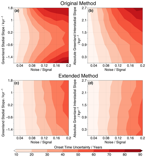
Figure A2 The onset time uncertainty, as measured by the width of the 5 %–95 % credible interval, for different combinations of noise and slope parameters. We consider both the original and extended implementations of the ramp-fitting method as applied to synthetic transitions with decadal resolution. Each panel contains 100 unique sets of parameter values, and for each set, we take the event mean over 100 synthetic transitions. When not explicitly varied, parameters are fixed at standard values as given in Sect. 3.1.

By having a model for the underlying transition, a noise process to represent short-term climate variability, and a set of prior probabilities, the final quantity we need to produce our posterior distributions is a likelihood function. This measures the likelihood of observing the data given a particular choice of model parameters. To do so, we decompose the observed data x_i into a deterministic component ${\widehat{x}}_i$ and a noise component ϵ_i, $x_i={\widehat{x}}_i+{\mathit{ϵ}}_i$. The likelihood function is then

$$\begin{array}{}\text{(A14)}& p\left({\mathit{ϵ}}_{i+\mathrm{1}}|{\mathit{ϵ}}_i,t_{i+\mathrm{1}},t_i,\mathit{\sigma },\mathit{\tau }\right)=\mathcal{N}\left({\mathit{ϵ}}_i\exp \left(-{\displaystyle \frac{t_{i+\mathrm{1}}-t_i}{\mathit{\tau }}}\right),{\mathit{\sigma }}_{\mathrm{eff},i}^{\mathrm{2}}\right).\end{array}$$

Together with the prior distributions, the likelihood function defines the posterior distribution p(θ|𝒟) up to a constant. Since this distribution is six-dimensional, it is computationally very expensive to perform any subsequent analysis. To circumvent this, an MCMC algorithm is used to sample a representative set from p(θ|𝒟). All results presented in this paper are based on the application of the computations to corresponding representative sets.

This initial formulation of the ramp-fitting method is very successful when applied to transitions that do not show a large gradient either before or after the transition, as is the case for most of the ice core data for which this method was originally developed. However, some model transitions show a much more exaggerated saw-toothed shape, with a strongly negative gradient, following the abrupt warming event. In these cases, the original formulation of the method performs poorly or sometimes fails entirely.

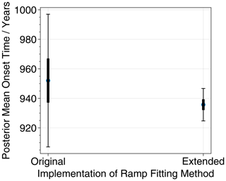
Figure A3 The posterior mean onset times for an AMOC transition in the CCSM4 model in both the original and extended implementations of the ramp-fitting method when using 25 different search windows. The extended implementation shows a reduced spread in the posterior mean onset times, indicating reduced sensitivity to the choice of search window.

We need to ensure that we can successfully characterise the full range of transitions within model simulations. To this end, we extend the original Erhardt method to include gradients before and after the transition with the addition of two new parameters, taking the total to eight. These are slope_GS, the gradient in the stadial prior to the DO event, and slope_GIS, the gradient in the following interstadial. This allows us to more accurately capture the shape of the transitions. Rather than being the initial value of the observations, y₀ is now the observed value at the start of the transition. The other parameters retain their original meanings, and the noise process is unchanged. With this extension, the deterministic component of the model is now described by the following equation:

$$\begin{array}{}\text{(A15)}& {\widehat{x}}_i\left(t_i\right)=\left\{\begin{array}{ll}{x}_{\mathrm{0}}-{\mathrm{slope}}_{\mathrm{GS}}\left(t_{\mathrm{0}}-t_i\right),& \mathrm{if}{t}_i\le t_{\mathrm{0}}\\ x_{\mathrm{0}}+\mathrm{\Delta }x\frac{t_i-t_{\mathrm{0}}}{\mathrm{\Delta }t},& \mathrm{if}{t}_{\mathrm{0}}<t_i<t_{\mathrm{1}}\\ x_{\mathrm{0}}+\mathrm{\Delta }x+{\mathrm{slope}}_{\mathrm{GIS}}\left(t_i-t_{\mathrm{1}}\right),& \mathrm{if}{t}_i\ge t_{\mathrm{1}}\end{array}\right..\end{array}$$

Our initial guesses for these two new parameters are zero, and the prior probabilities, which are identical, are chosen to avoid gradients in the stadial or interstadial which are greater than those during the transition itself.

$$\begin{array}{}\text{(A16)}& p\left({\mathrm{slope}}_{\mathrm{GS}}\right)=p\left({\mathrm{slope}}_{\mathrm{GIS}}\right)=\mathcal{N}\left(\mathrm{0.0},{\displaystyle \frac{\left|\mathrm{\Delta }x\right|}{\mathrm{10}\mathrm{\Delta }t}}\right)\end{array}$$

The prior probabilities for the other six parameters remain unchanged, as does the likelihood function.

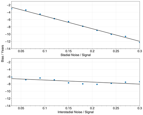
We assess the performance of both the original and extended implementations of the ramp-fitting method using decadal-resolution synthetic transitions generated as described in Sect. 3.1 for different values of the noise $/$ signal, Greenland stadial slope, and Greenland interstadial slope. Our performance metric is the uncertainty in the transition onset time, which we quantify as the width of the 5 %–95 % credible interval. We take an event mean across 100 synthetic transitions for each set of parameters to reduce the impact of random variability.

For cases of small slopes and large noise $/$ signal, for example, comparing the lower-right corners of Fig. A2b and d, we find that the original method outperforms our extended method in that it has lower uncertainty in the onset time. This is unsurprising, as in these cases we have essentially introduced two unnecessary parameters. However, for cases where meaningful slopes are present, our extended method outperforms the original method.

We also test the sensitivity to the choice of search window for the two implementations of the ramp-fitting method. Choosing an AMOC transition from the CCSM4 model, we calculate the posterior mean onset time using 25 different search windows for both the original and extended implementations. Figure A3 shows that the spread of these posterior mean onset times is much lower in our extended method than in the original method, with the standard deviation reduced from 24.7 to 6.4 years. This indicates that, at least for a case where noticeable slopes are present before or after the transition, our extended method is less sensitive to the choice of search window.

Finally, we test the accuracy of the posterior mean estimates from our extended method of the autocorrelation time, Greenland stadial slope, Greenland interstadial slope, and transition duration under very low levels of noise. Varying only one parameter at a time, we find largely accurate estimates of these parameters (Fig. A4). The exceptions are the autocorrelation time, which is consistently slightly overestimated, and the stadial slope, where our extended method leads to an overestimate for cases in which the true stadial slope is strongly negative.

In addition to the original and extended implementations which are the focus of this work, we also consider an implementation of the ramp-fitting method using an alternative set of prior probabilities similar to those employed by Capron et al. (2021). The key difference here is that the prior probabilities for the transition onset time t₀ and the transition duration Δt are uniform. This implementation includes the slopes slope_GS and slope_GIS discussed above, and aside from the uniform priors, there are no further differences.

Figure A4 Low noise benchmarks of our extended ramp-fitting method. Varying only one parameter at a time, we plot true values against estimated values for (a) autocorrelation time, (b) Greenland stadial slope, (c) Greenland interstadial slope, and (d) transition duration. The noise $/$ signal ratio is set to 0.01, and when not explicitly varied, the other parameters are fixed at their standard values as given in Sect. 3.1. Each data point is given by the event mean across 100 synthetic transitions of the posterior mean for that parameter.

Appendix B: Hypothesis test

After the bias correction, the event-averaged lead of the precipitation's transition is approximately symmetrically uncertainty-distributed around −10.0 years, with the 95 % confidence interval reaching from −3.9 to −16.5 years.

In order to assess significance of this result, we test the following competing hypotheses:

• H₀, where the population mean time lag for precipitation relative to temperature is equal to zero. The observed (uncorrected) precipitation lead is a spurious result induced by the method.

• H₁, where the population mean time lag for precipitation relative to temperature is not equal to zero.

To test these hypothesis against each other, we design an empirical null distribution. Our null distribution will reflect the plausibility that the ramp fit assigns to a certain event-averaged (over 19 events) temporal lag 〈Δt〉₁₉, given that the null hypothesis is true. (The randomness associated with the individual time series involved in the computation of 〈Δt〉₁₉ is integrated out in our null hypothesis.) We then compare the uncertainty distribution obtained from the assessment of the CCSM4 data with this null distribution. In a slight abuse of terminology, we compute a corresponding p value as the probability that any $\langle \mathrm{\Delta }t{\rangle }_{\mathrm{19}}^{\mathrm{obs}}$ sampled from the observed uncertainty distribution is closer to the mean of the null distribution μ₀ than a second one $\langle \mathrm{\Delta }t{\rangle }_{\mathrm{19}}^{\mathrm{null}}$ sampled from the null distribution.

$$\begin{array}{}\text{(B1)}& p=P\left(|\langle \mathrm{\Delta }t{\rangle }_{\mathrm{19}}^{\mathrm{obs}}-{\mathit{\mu }}_{\mathrm{null}}|<|\langle \mathrm{\Delta }t{\rangle }_{\mathrm{19}}^{\mathrm{null}}-{\mathit{\mu }}_{\mathrm{null}}|\right)=\mathrm{0.078}\end{array}$$

To construct this distribution, we randomly sample 19 pairs of time series from the analogous synthetic transitions for precipitation and temperature. Application of the ramp fit to the individual pairs yields 19 uncertain time lags. From each of these 19 uncertainty distributions, we sample a single value and subsequently perform the event average. A 100 000-fold repetition of this procedure yields a set of time lags averaged over 19 events that reflects the randomness in the 19-fold observation of the random experiment “DO event” and the uncertainty in the timing of each transition onset.

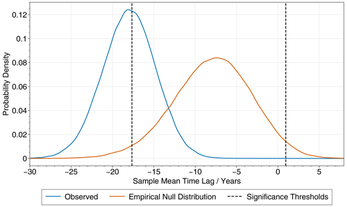
Figure B1 The observed and empirical null distributions for the sample mean time lag between precipitation and temperature in the CCSM4 model. The observed distribution here is identical to the uncorrected distribution in Fig. 4. In total, 5 % of the empirical null distribution lies outside of the significance thresholds shown as dashed lines.

Appendix C: Additional figures

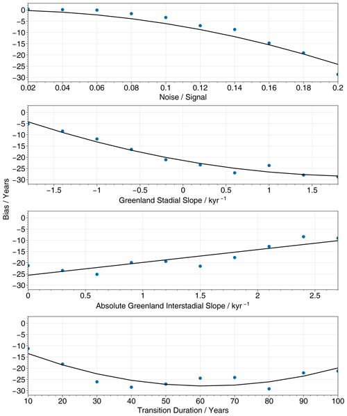
Figure C1 The dependence of the transition onset time bias on four transition parameters when using our extended ramp-fitting method with uniform priors, similar to those adopted by Capron et al. (2021), for transitions with decadal resolution. For further details, see Appendix A. When not explicitly varied, the noise $/$ signal ratio is fixed at 0.2, and the other parameters are fixed at standard values as given in Sect. 3.1. The bias is greater than when using our standard priors (Fig. 3).

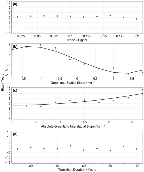
Figure C2 The dependence of the bias on four transition parameters when using a simple least squares method instead of the Bayesian fitting method for transitions with a decadal resolution. When not explicitly varied, the noise $/$ signal ratio is fixed at 0.2, and the other parameters are fixed at standard values as given in Sect. 3.1. No trend is plotted for the noise $/$ signal ratio or for the duration, as the bias does not significantly depend on these parameters. However, there is a strong non-linear dependence of the bias on the slopes.

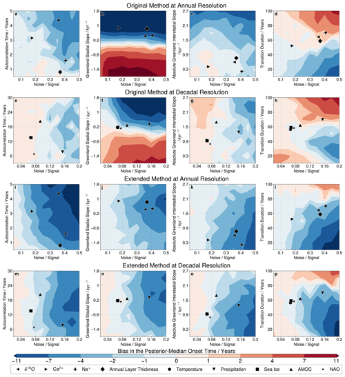
Figure C3 The bias in the posterior median transition onset time is calculated following the same approach as for the posterior mean in Fig. 3. Considering the posterior median onset time instead of the posterior mean leads to slightly more positive values of the bias, but the difference is small.

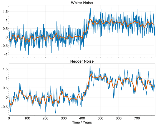
Figure C4 Examples of how we down-sample the annual-resolution synthetic data to decadal resolution for the cases of both whiter and redder noise.

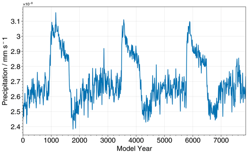
Figure C5 The time series for precipitation in the CCSM4 simulation with 200 ppm of atmospheric carbon dioxide, demonstrating the relatively higher level of noise during the cooler stadial periods, which are visible here as periods of lower precipitation.

Figure C6 The dependence of the bias on noise $/$ signal in both the preceding stadial and following interstadial for the case of two independent noise regimes. The bias depends much more on the stadial noise $/$ signal.

Appendix D: Transition parameters for bias estimation

We present here the minimum, event mean, and maximum values, across the sample of DO events, of the posterior mean transition parameters for all of the CCSM4 variables (Table D1) and NGRIP proxies (Table D2) considered in this study, as given by the extended ramp-fitting method. These values are used to generate the “analogous” synthetic transitions which we use to estimate the bias affecting each variable or proxy, with one exception for NGRIP as follows. We convert each posterior mean autocorrelation time into an autocorrelation parameter α, and then convert the event mean of α back into an autocorrelation time using the appropriate time resolution. We do this because we find that the autocorrelation time is correlated with the temporal resolution, whereas α is not, and so it is more appropriate to take our mean over α.

For the CCSM4 model data, all of the slopes during the interstadials following the transition are negative, and so we give the absolute values as in Fig. 3. However, for the NGRIP data, there are a small number of cases where this slope is in fact positive, and so for NGRIP we do not give the absolute values.

The minima and maxima of the different transitions parameters are used to select plausible parameter ranges over which to perform the systematic testing in Sect. 3.1.

Table D1 The minimum, event mean, and maximum of the posterior mean parameter values for each variable across the sample of 19 abrupt warming events in the CCSM4 model simulations. The mean values are used to construct the synthetic transitions with which we estimate bias, as described in Sect. 3.3.

Table D2 The minimum, event mean, and maximum of the posterior mean parameter values for each proxy across the sample of 16 DO events in the NGRIP ice core record. The mean values are used to construct the synthetic transitions with which we estimate bias, as described in Sect. 3.3.