the Creative Commons Attribution 4.0 License.
the Creative Commons Attribution 4.0 License.
 | 30 Aug 2024
Carbonyl sulfide measurements from a South Pole ice core and implications for atmospheric variability since the last glacial period
Melinda R. Nicewonger
Gregory L. Britten
Dominic Winski
Mary Whelan
John D. Patterson
Erich Osterberg
Christopher F. Lee
Tara Harder
Kyle J. Callahan
David Ferris
Eric S. Saltzman
Carbonyl sulfide (COS) is the most abundant sulfur gas in the atmosphere with links to terrestrial and oceanic productivity. We measured COS in ice core air from an intermediate-depth ice core from the South Pole using both dry and wet extraction methods, recovering a 52 500-year record. We find evidence for COS production in the firn, altering the atmospheric signal preserved in the ice core. Mean sea salt aerosol concentrations from the same depth are a good proxy for the COS production, which disproportionately impacts the measurements from glacial period ice with high sea salt aerosol concentrations. The COS measurements are corrected using sea salt sodium (ssNa) as a proxy for the excess COS resulting from the production. The ssNa-corrected COS record displays substantially less COS in the glacial period atmosphere than the Holocene and a 2 to 4-fold COS rise during the deglaciation synchronous with the associated climate signal. The deglacial COS rise was primarily source driven. Oceanic emissions in the form of COS, carbon disulfide (CS2), and dimethylsulfide (DMS) are collectively the largest natural source of atmospheric COS. A large increase in ocean COS emissions during the deglaciation suggests enhancements in emissions of ocean sulfur gases via processes that involve ocean productivity, although we cannot quantify individual contributions from each gas.
- Article
(11366 KB) - Full-text XML
-
Supplement
(449 KB) - BibTeX
- EndNote


The sources of atmospheric carbonyl sulfide (COS) include anthropogenic activities, oceans, biomass burning, anoxic ecosystems, and volcanism (Berry et al., 2013; Kettle et al., 2002; Whelan et al., 2018). Present-day global mean levels are 480–490 pmol mol−1 (ppt) (Montzka et al., 2007), with anthropogenic emissions accounting for about 40 % of emissions (Table 1). The oceans are the largest natural source, which include direct emissions in the form of COS and indirect emissions in the form of precursor gases carbon disulfide (CS2) and dimethylsulfide (C2H6S or DMS), whose atmospheric oxidation products include COS (Berry et al., 2013; Kettle et al., 2002; Jernigan et al., 2022; Lennartz et al., 2017, 2019; Whelan et al., 2018). In the ocean, COS and CS2 are produced primarily by photochemical reactions involving organosulfur compounds (Kettle et al., 2002; Lennartz et al., 2017, 2019; Whelan et al., 2018), and DMS is a byproduct of phytoplanktonic activity (Andreae, 1990; Charlson et al., 1987; Ksionzek et al., 2016; Lana et al., 2011; Vogt and Liss, 2009; Wang et al., 2018a). Warmer waters can act as a seasonal sink due to temperature-dependent loss to hydrolysis, but the world oceans are a large net source on an annual average basis with respect to both the direct and indirect emissions (Kettle et al., 2002; Lennartz et al., 2017, 2020). Biomass burning, anoxic wetlands, and volcanism are considered minor sources (Berry et al., 2013; Kettle et al., 2002; Montzka et al., 2007; Whelan et al., 2018). The primary removal mechanism of atmospheric COS is uptake by terrestrial plants during photosynthesis, which accounts for 70 %–80 % of total atmospheric removal of COS (Table 1). The remaining losses are attributed to soil uptake, atmospheric oxidation via OH, direct photolysis in the atmosphere, and stratospheric loss, resulting in a tropospheric lifetime of 2–3 years (Berry et al., 2013; Kettle et al., 2002; Montzka et al., 2007; Whelan et al., 2018).
Table 1Atmospheric COS budget.
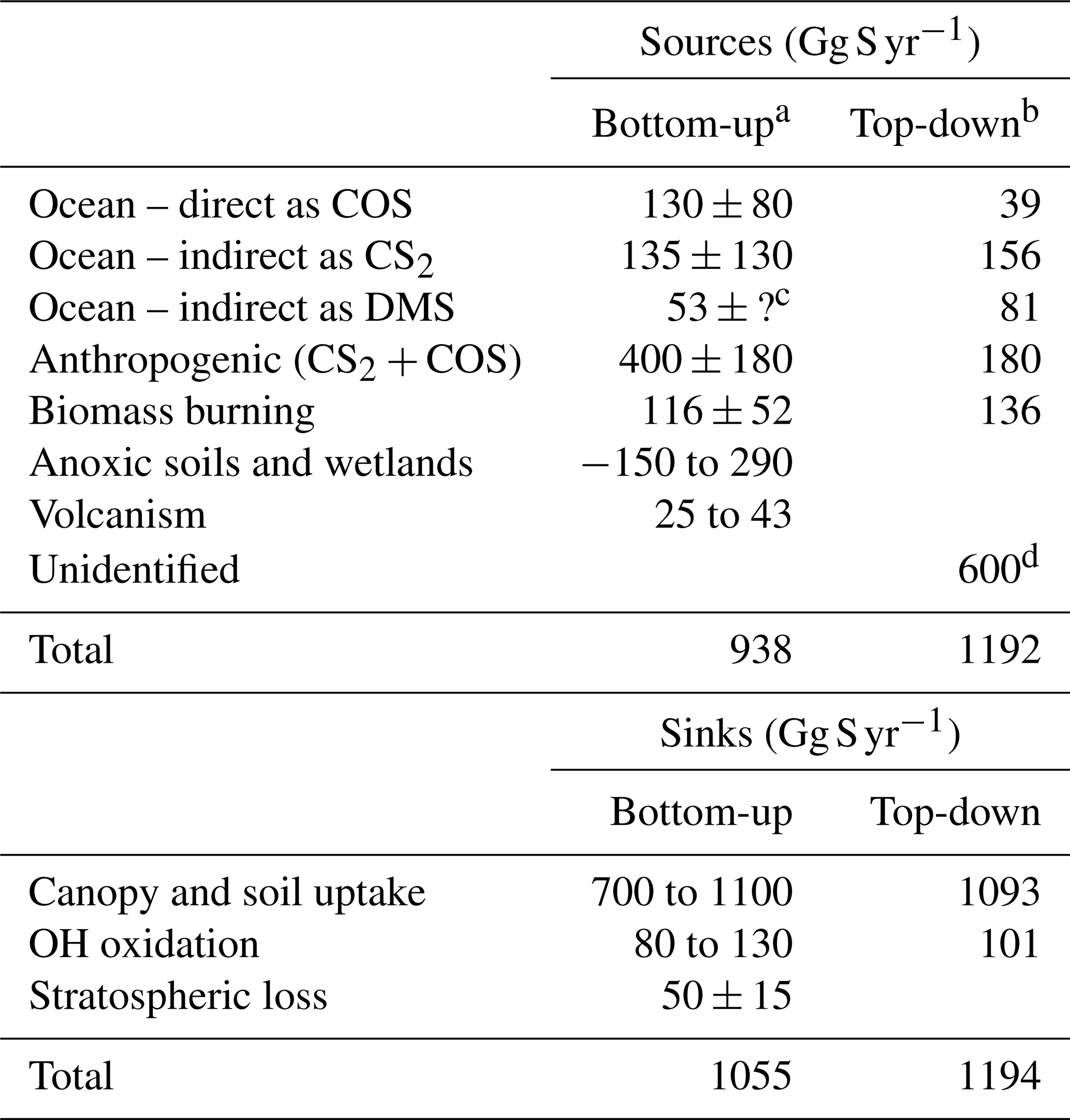
a Whelan et al. (2018). b Berry et al. (2013). c Based on mechanistic modeling in Jernigan et al. (2022), the uncertainty is not quantified. d Presumed to be photochemical and attributed to low-latitude oceans.
Past atmospheric variability of COS is of interest because COS is a precursor for background stratospheric sulfate aerosol with impacts on stratospheric chemistry and a net negative radiative impact (Kremser et al., 2016; Quaglia et al., 2022; Sheng et al., 2015; Solomon, 1999). Further, atmospheric COS is associated with oceanic production and emission of DMS, which is a major source of marine sulfate aerosol, inducing negative direct and indirect climate feedbacks (Boucher et al., 2013; Thomas et al., 2010; Wang et al., 2018b). Polar ice cores contain ancient air that can be used to reconstruct past atmospheric composition of trace gases. Previous measurements of COS in Antarctic ice cores revealed slow, temperature-dependent degradation of COS in the ice core air due to hydrolysis (Aydin et al., 2014). The kinetic parameters of the in situ COS loss have been estimated, allowing reconstruction of a 54 000-year composite ice core COS record based on data from multiple Antarctic sites including glacial period measurements from the West Antarctic Ice Sheet (WAIS) Divide and Taylor Dome sites (Aydin et al., 2016).
The existing composite ice core record had multiple limitations (Aydin et al., 2016). First, the measurements from ice with warmer temperature histories require large corrections for loss. Second, the measurements from the bubble–clathrate transition zone (BCTZ) at the WAIS Divide site displayed large negative biases; the BCTZ refers to the depth range over which the air inclusions in the ice transition from gas phase (bubbles) to air hydrate clathrates (clathrates) due to increasing hydrostatic pressure (Ikeda et al., 1999). Third, the temporal resolution of measurements from either ice core was low over broad age horizons, and the chronology of the Taylor Dome ice core was highly uncertain during the glacial period and the glacial–interglacial transition. While the data from the two ice core sites displayed lower levels early in the glacial period than the Holocene in agreement with each other, they trended in different directions during the deglaciation, complicating the atmospheric interpretation of the record (Sect. 3). Measurements from other ice cores were necessary to determine whether the discrepancies were solely due to unquantified uncertainties associated with the known limitations or if there were unidentified problems such as production processes altering ice core COS levels.
In this work, we present new measurements from the intermediate-depth SPC14 ice core recently drilled to 1751 m at the South Pole as part of the SPICEcore project (Souney et al., 2020). These measurements were conducted at considerably higher resolution than the prior data sets, resulting in a continuous ice core COS record spanning the 52.5 ka (kiloannum) before present (1950 CE), and the cold mean annual surface temperatures at the South Pole (−50 °C) mean that measurements do not require a correction for loss to hydrolysis (Aydin et al., 2014, 2016). These characteristics allow evaluation of the SPC14 measurements with respect to possible impurity-related production in the ice sheet, resulting in excess (not of atmospheric origin) COS. Presence of excess COS can impede the recovery of an atmospheric record from the ice core measurements. This is particularly relevant for measurements from glacial period ice, which typically contain high concentrations of ice impurities. Here, we rely on measurements of soluble ions Ca2+ and Na+ (Winski et al., 2021) as indicators for land- and marine-sourced ice impurities to check for the presence of excess COS in the SPC14 ice core. We find compelling evidence for presence of excess COS through the entire SPC14 ice core. The amount of excess COS is quantified and corrected for using linear regression analyses between sea salt Na (ssNa) and COS, resulting in an inferred atmospheric record of COS. We implement a Bayesian approach within a state-of-the-art numerical framework to quantify and propagate the full range of uncertainty arising from the corrections to the atmospheric COS record. The atmospheric record is interpreted rigorously within the uncertainties, relying on the contemporary knowledge of the atmospheric COS budget.
2.1 Dry- and wet-extraction-based COS analysis
All COS measurements were conducted at the UCI ice core trace gas laboratory. We analyzed 10–20 cm long samples from the designated gas cross-section of the SPC14 ice core. Air entrapped in the ice core samples is extracted using dry (frozen) and wet (melt) extraction methods that have been previously used for ice core measurements of COS and other trace gases (Aydin et al., 2007, 2014, 2016; Nicewonger et al., 2016). In dry extraction, ice core air is liberated via mechanical shredding of frozen ice samples in four identical stainless-steel vacuum chambers (6 L), each fitted with a flat, sharp cutting surface. Samples are placed on the cutters inside the vacuum chambers and shredded by linear oscillations (15 cm throw at 1 Hz for 20 min) inside a −50 °C freezer. In wet extraction, ice core air is liberated by melting the samples in two identical glass vessels at 30 °C, which typically takes 30–40 min. The SPC14 dry-extraction samples were 400–500 g, and wet-extraction samples were 300–350 g. Melting releases more than 99 % of the ice core air (Nicewonger et al., 2020). The dry-extraction efficiency for the UCI dry-extraction vessels is about 60 % for bubbly ice samples and 40 % for full clathrate ice, with an expected drop in the extracted air amount across the BCTZ (Aydin et al., 2016). The clathrates are smaller in size than bubbles and harder than ice (Ohno et al., 2004; Salamatin et al., 1998); the relatively lower extraction efficiency of the dry extraction method for clathrates vs. bubbles is presumed to be primarily due to a combination of these two factors.
In the BCTZ, the gas composition of the air in bubble and clathrate phases can display extreme fractionation likely due to different diffusive fluxes for different gases during the transition process, and at the completion of the transition, the composition of the air hydrates is expected to reflect atmospheric levels (Ikeda et al., 1999; Ikeda-Fukazawa et al., 2001; Ohno et al., 2004). Dry-extraction-based measurements from the WAIS Divide ice core suggest dry COS measurements are prone to low bias and higher scatter in the BCTZ, suggesting the bubbles, which are extracted more efficiently than the clathrates, are depleted with respect to COS (Aydin et al., 2016). The SPC14 data set does not include any dry measurements from the initially anticipated BCTZ zone (900–1200 m); this sampling strategy was designed to avoid the measurement artifacts associated with the low extraction efficiency of dry extraction (Fig. 1a). In the SPC14 dry extractions, the amount of air extracted from the samples start to drop at 800 m (Appendix Fig. A1a), suggesting the BCTZ starts about 100 m above the initially anticipated depth of 900 m.
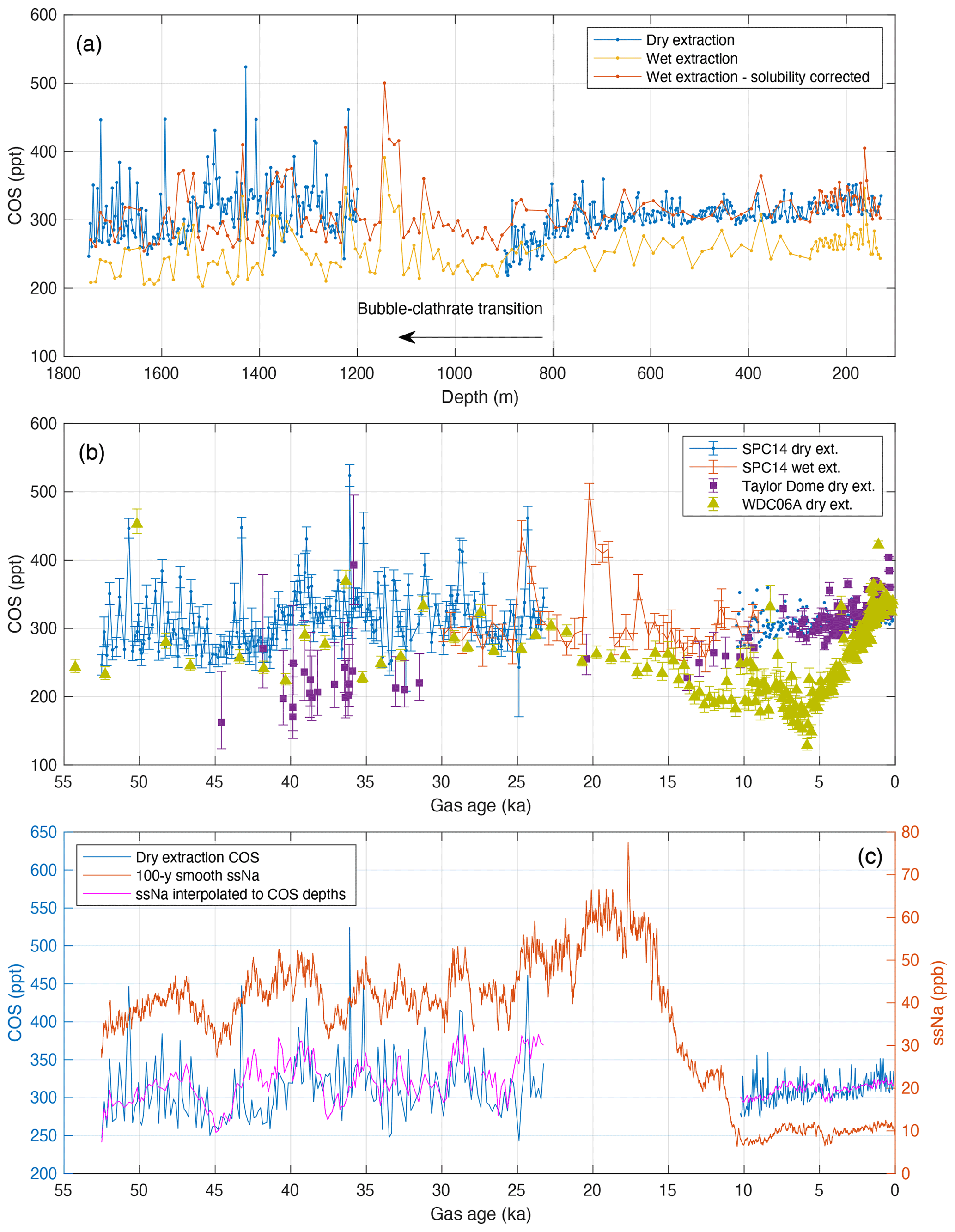
Figure 1(a) COS measurements based on dry (blue) and wet (yellow) extraction methods and solubility-corrected wet-extraction data (red) vs. depth in the SPC14 ice core. The dry measurements from the BCTZ (dashed line) are excluded from the interpretation. (b) COS measurements from the SPC14 (blue and red), Taylor Dome (purple), and WAIS Divide (green) ice cores vs. gas age. Only a subset of the wet SPC14 data from 30–9 ka is shown because dry measurements are preferred when there are data from both extraction methods. (c) Dry COS measurements for the SPC14 ice core (blue) are on the left y axis, while the 100-year smooth ssNa (red) measurements are on the right y axis. The ssNa interpolated to COS measurement depths (magenta) are shown with an offset of −20 ppb below 1200 m and +10 ppb above 800 m.
The wet-extraction system and methods have been developed for non-methane hydrocarbon measurements (Nicewonger et al., 2016, 2020) and the SPC14 measurements presented here are the first COS data from the wet-extraction system. BCTZ does not represent a problem for the wet measurements because of the >99 % efficiency of this extraction method. However, COS is more soluble in water than air, resulting in a negative bias in wet measurements (Fig. 1a) which has to be corrected for (Sect. 2.2).
Following either wet or dry extraction, the sample air is frozen in a stainless-steel tube dipped in liquid helium (4 K) for transfer to the analysis inlet system used for pre-concentration of the trace gases followed by GC-MS (gas chromatography–mass spectrometry) analysis. COS is measured with the same analytical instrumentation regardless of the ice core air extraction method. Trace gases including COS are pre-concentrated on a glass-bead trap using liquid nitrogen (77 K), followed by transfer onto a capillary trap (77 K) before being thermally injected onto a DB-1 GC column. The GC is connected to a dual-focusing magnetic sector MS that operates at a mass resolution () of 8000–10 000 at 5 % peak height. The GC-MS system is calibrated with an isotope dilution technique using a 13C-labeled COS isotope standard (13COS) along with ppt-level unlabeled 12COS standards. Both labeled and unlabeled ppt-level standards are prepared in our laboratory from ppb-level primary (long term) standards. The primary standards are also prepared in our laboratory from commercially available pure gases. A known amount of ppt-level 13COS internal standard is mixed with every sample during the pre-concentration step and co-analyzed with the COS from the sample ice core air.
All measurements are reported as dry molar mixing ratios and are corrected for 2 % gravitational enrichment based on hydrostatic equilibrium at the present-day firn close-off depth of 120 m at the South Pole. For simplicity, we ignore temporal variability in the gravitational correction. The errors arising from this simplification should be less than 1 % of the reported mixing ratios.
2.2 Solubility correction for the wet-extraction measurements
We calculate the solubility correction empirically for each sample and correct the wet measurements. The ratio of total moles of COS to what is left in the ice core meltwater during wet extraction can be calculated by (Nicewonger et al., 2020)
In Eq. (1), mt is the total moles of COS, ml is moles of COS left dissolved in the meltwater, Vg is the volume of the gas (headspace) in the melt chamber, Vl is the volume of the meltwater, and h is the dimensionless effective solubility (aqueous concentration divided by gas concentration). We assume h to be the same for every sample melt. Vg can be substituted by volume of the melt chamber (Vc) minus Vl, and Eq. (1) can be rearranged into expressing as a linear function of a single variable (Vl) and two constants (C1 and C2), given that Vc is also constant:
On the left side of Eq. (2), mt scales with the dry-extraction COS mixing ratio (COSdry), and ml scales with the difference between the dry- and wet-extraction (COSwet) mixing ratios at the same depth, assuming solubility of air in the meltwater is negligible compared to that of COS. Nicewonger et al. (2020) estimated 0.7 % of the air could be left in the meltwater for an average size sample at saturation equilibrium. The dry-extraction mixing ratio at a given depth is estimated by linear interpolation from the smoothed dry-extraction record (Fig. A2). The Vl on the right-hand side of Eq. (2) scales with the weight of the ice samples (Wts), assuming sample-to-sample density variations are negligible. The Eq. (2) can be rearranged to
C3 and C4 are constants that can be estimated from the linear regression of the inverse of Wts vs. the left-hand side of Eq. (3) using data from above 720 m (Fig. A2). We use a Bayesian errors-in-variables linear regression to estimate the solubility correction for the SPC14 wet-extraction data due to nonuniform errors, although a least-squares linear regression yields similar results (Fig. A3). The errors-in-variables regression is conducted within a hierarchical Bayesian framework using the Stan probabilistic software package (https://mc-stan.org/, last access: 19 August 2024), in which all uncertain parameters are interpreted probabilistically (Carpenter et al., 2017). Stan uses efficient Hamiltonian Markov Chain Monte Carlo (HMC) sampling. The Bayesian model assumes distributions for the x variable () using Eq. (4) as follows:
which describes the measured x as normally distributed with a mean equal to the true x and standard deviation xerr. The probability distribution of the linear relationship between x and y (left-hand side of Eq. 3) variables is described by Eq. (5):
where parameters b and a are the unknown intercept (C3) and slope (C4) of the linear relationship. We do not impose any a priori limits on the parameters a and b. The true x parameter is required to be positive because sample weight cannot be less than zero. The posterior probability distributions are calculated via the Stan code (code in the Supplement) as executed in cmdStan 2.34.1 (https://github.com/stan-dev/cmdstan/releases, last access: 19 August 2024). The HMC code uses four chains with 2000 iterations each for a total of 8000 evaluations of the posterior probability. The HMC diagnostic split achieved for the four chains, indicating convergence.
Once C3 and C4 are known, the solubility correction for wet-extraction measurements can be estimated by inserting the COSwet and Wts data into Eq. (3) to calculate the solubility-corrected COS mixing ratio represented by COSdry in Eq. (3). The calculations are carried out within the generated quantities block of the Stan code (code in the Supplement) using the full probability distributions of C3 and C4 and the uncertainty distributions of the x and y data. This allows for the propagation of all measurement and parametric uncertainty to the corrected wet-extraction COS record. The average solubility correction () is a factor of 1.20 for samples shallower than 720 m and 1.23 for samples deeper than 720 m (Fig. A3).
2.3 Calculation of ssNa and nssCa
We use established methods to infer the source contributions of Na+ and Ca2+ ions for the SPC14 ice core (Winski et al., 2021). We partition Na+ and Ca2+ into sources from marine and crustal origin based on the respective mass ratios of 0.038 and 1.78 (Bowen, 1979). Given these ratios and assuming that the sum of marine and terrestrial Na+ and Ca2+ equals what is measured in the laboratory, we use
where Rm=0.038, Rt=1.78, nssCa2+ is terrestrial non-sea salt Ca2+, and ssNa+ is sea salt Na+; ssNa and nssCa are commonly used as reliable proxies for ice core impurities of terrestrial and marine origin (Fischer et al., 2007).
2.4 Bayesian methods for errors-in-variables regressions of ssNa vs. COS
We use errors-in-variables regression analyses between sea salt Na (ssNa) and COS to quantify the excess COS amount, correct the measurements, and recover the underlying atmospheric record. All errors-in-variables linear regression analyses are conducted within the same hierarchical Bayesian framework as the solubility corrections, using the Stan probabilistic software package. The Bayesian model assumes distributions for the x variable based on Eq. (4). The probability distribution incorporating the linear relationship between x (ssNa) and y (COS) variables is characterized by Eq. (8):
which only differs from Eq. (5) in that it includes α as a third parameter scaling the y-variable errors as needed depending on various analysis scenarios used in the ssNa vs. COS regressions (Table 2). The error estimates for the COS and ssNa measurements (Sect. 2.5) are directly incorporated in the errors-in-variables regressions as they substitute for yerr and xerr in Eqs. (4) and (8), allowing us to propagate the uncertainty in the measurements to the slope of the relationship between ssNa and COS. Various data treatment decisions made during the data analysis may act as additional sources of uncertainty. To address this concern, we use different analysis scenarios, four for the glacial period (G1 through G4 in Table 2) and two for the Holocene (H1 and H2 in Table 2), making different data treatment decisions. The factors considered in construction of the different analysis scenarios include (1) different smoothing methods for COS and ssNa to minimize the impact of uncorrelated high-frequency variability in ssNa and COS; (2) different approaches to estimating the measurement uncertainties, including scaling them up, and therefore determining the sensitivity of results to the uncertainty in the uncertainty estimates; and (3) conducting simultaneous same-depth and same-age regressions in G4 and H2 to account for the underlying atmospheric COS variability while quantifying the ssNa correction, which should yield a more realistic range for atmospheric COS variability. The corrections are conducted using the full slope probability distribution functions (PDFs) for all analysis scenarios, and the results are presented in Sect. 3.1.
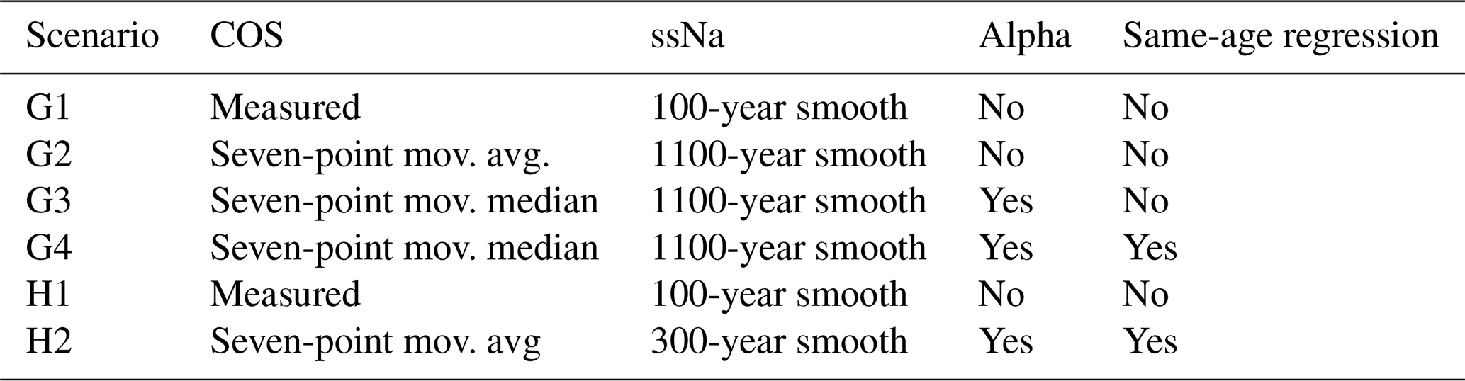
We do not impose any a priori limits on the a and b parameters. The true x (xtrue) parameter is required to be positive in the all regressions because ssNa cannot be less than zero. In three of the analysis scenarios (G1, G2, H1), the α parameter is constrained to a constant value 1, meaning the estimated y-variable uncertainties were not scaled in the Bayesian inference. The G3 regression includes an unconstrained α. The G4 and H2 regressions include simultaneous regressions of the same-depth (co-registered quantities from the same depth in the ice core) and same-age (quantities from the same ice and gas ages) relationships between ssNa and COS and the unconstrained α (Table 2). Inclusion of the α parameter allows evaluation of the sensitivity of the correction slope to possible bias of COS measurement errors. The simultaneous regression algorithm includes two instances of the Eq. (4), and two interdependent equations replace Eq. (8), characterizing the linear relationship for the same-depth and the same-age analyses:
The simultaneous regression includes six unknowns: x1 and x2 represent the true x from Eq. (4) for the same-depth and same-age regressions, while a1, a2, b1, and b2 are slopes and intercepts for the same-depth and same-age regressions. The model accounts for the relationships in both spaces by estimating the parameters simultaneously. The simultaneous regression algorithm is the most complex Stan code used in our analyses (code in the Supplement). Simplified versions were used as needed for the different analysis scenarios described in Table 2. The regressions were conducted with cmdStan 2.34.1 (https://github.com/stan-dev/cmdstan/releases, last access: 19 August 2024) using four chains with 2000 iterations each, for a total of 8000 evaluations of the posterior probability. The HMC diagnostic split (a measure of convergence between and within chains) of the slope posteriors for the G1, G2, G3, G4, H1, and H2 scenarios achieved with respective effective sample sizes (Neff) of 4900, 2500, 7100, 3900, 3900, and 4700. The convergence criteria are met when at Neff>400 (Vehtari et al., 2021). The same diagnostics for all other Stan-based regressions also indicate convergence.
All slope PDFs shown in the paper display the posteriors of the slope parameter from the Bayesian inference. We also estimate a probability range for the corrected COS records for all regressions using the “generated quantities” block of the Stan code (code in the Supplement), accounting for the full range of uncertainties that arise from the slope PDFs and the x-variable ssNa. The 2σ uncertainty ranges shown in the Figs. 4b and 5 represent ±2 SD of the posterior probability distributions.
2.5 COS and ssNa errors for the Bayesian linear regression analyses
There are two primary factors that contribute to the error estimates of the individual COS measurements (Aydin et al., 2007). The first one is the uncertainty that arises from the reproducibility of calibration curves. A typical COS calibration curve for the GC-MS system is more uncertain at the low end of its dynamic range. This results in larger relative errors for lower COS mixing ratios and for smaller ice samples that yield less air for the analysis. The second factor is the background COS that is inherent to the extraction vessels and vacuum lines used for the ice core air extractions. The background COS is characterized by clean N2 analyses through the ice core extraction system, which is subsequently subtracted from the ice core sample signal. The variance in the background COS level introduces a larger relative uncertainty to smaller samples and lower mixing ratios that is much like the calibration curve uncertainty. As a result, the reported COS measurements have non-uniform errors.
The ssNa was measured continuously in the SPC14 ice core, leading to much higher data density than the COS measurements (Winski et al., 2021). We use a moving standard error of measurement means that fall within a time window (typically 100 years or higher and lower depending on the analysis scenario) to calculate the uncertainty in the ssNa concentration at the corresponding depth range in the ice core. The standard errors are calculated from unbiased (divided by N−1) standard deviations. There are on average 82 ssNa measurements per 100-year averaging window below 1200 m, which is the depth range corresponding to the glacial period dry-extraction measurements that constitute the basis for excess COS corrections.
COS was measured over the length of the SPC14 ice core with the shallowest samples from 129 m and the deepest from 1749.3 m depth (Fig. 1a). Out of a total of 574 measurements, 425 samples were analyzed by dry extraction and 149 by wet extraction. A solubility correction (∼20 % on average) is applied to all wet COS measurements (Fig. A3). No hydrolysis loss correction is applied to any of the SPC14 COS measurements. The solubility-corrected wet measurements exceed the 35 dry measurements in the 800–900 m range (Fig. 1a), indicating a depletion in these dry measurements due to the onset of the BCTZ. The onset of BCTZ around 800 m is also evident from the large drop in extracted gas amount, reflecting the associated decrease in gas extraction efficiency during dry extraction (Fig. A1a). These 35 measurements (0.6 % of the data set) are excluded from data analyses.
The remaining measurements (n=539) exhibit higher variability below 1035 m (16 ka in gas age), displaying a propensity for rapid positive excursions (spikes) of 100–150 ppt (Fig. 1a). Consequently, the distribution of the measurements prior to 16 ka is broad and skewed compared with the measurements from periods after 16 ka (Fig. 2a and b). Both dry and wet-extraction measurements prior to 16 ka display similarly skewed distributions, implying that the spikes do not result from inefficient gas extraction or another experimental artifact impacting the clathrate ice measurements. The atmospheric lifetime of COS (2–3 years) and the spectral width of the firn smoothing at the South Pole (50–80 years; Epifanio et al., 2020) are both shorter than the average resolution of the dry glacial period measurements (160 years); therefore, we cannot rule out the possibility that these spikes represent atmospheric variability. However, 100–150 ppt spikes imply 30 %–50 % changes in COS biogeochemistry over 100-year timescales, which is similar to the increase in atmospheric COS during the 20th century caused by anthropogenic activities (Aydin et al., 2020). It seems unlikely that the COS mixing ratio in the glacial period atmosphere varied abruptly at the magnitude and frequency of these spikes. There is a prominent peak in 1114–1144 m depth range characterized by four wet measurements that are considerably higher than the adjacent data and hence more likely to be indicative of an atmospheric peak than the shorter-lived spikes (Fig. 1a).
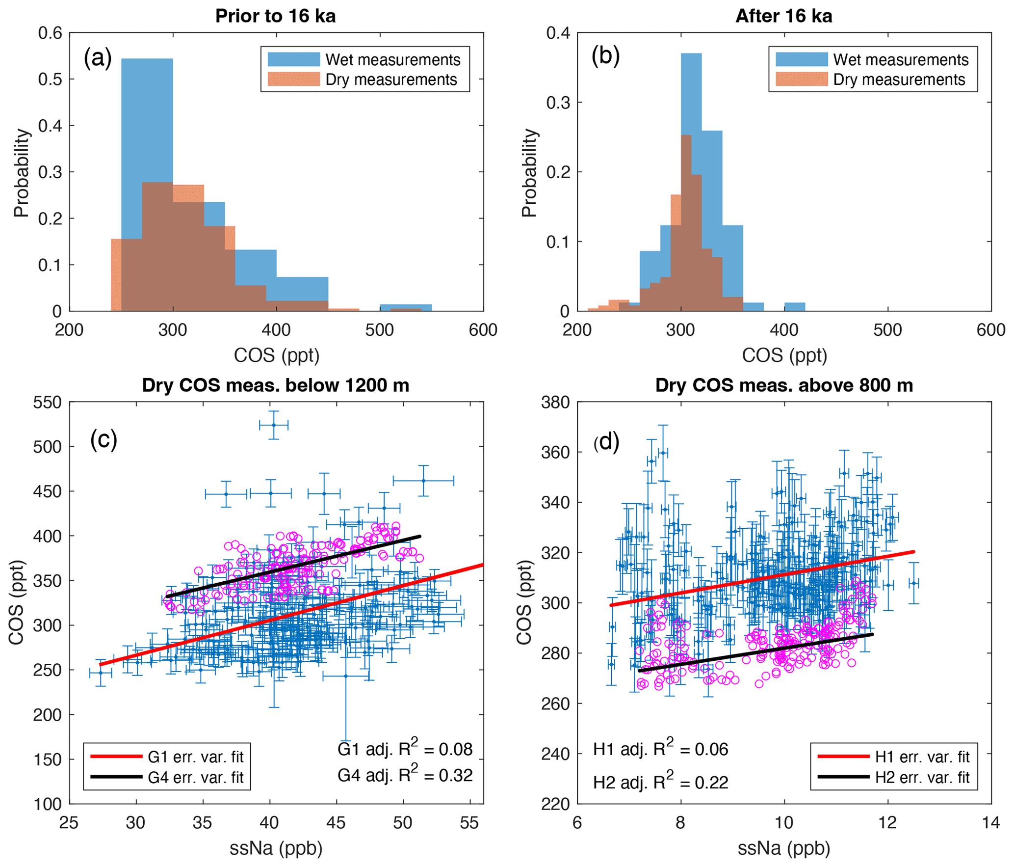
Figure 2(a) Distribution of SPC14 COS measurements before 16 ka. The dry measurements shown here are the basis for the regressions shown in (c). (b) Distribution of SPC14 COS measurements after 16 ka. The dry measurements shown here are the basis for the regressions shown in (d). (c) The ssNa vs. dry COS measurements for the glacial period (below 1200 m) used in the G1 (blue error bars) and the G4 (magenta circles) scenarios (Table 2). The linear fits to errors-in-variables regressions are calculated using the mean slopes and intercepts for G1 and G4 (also see Figs. A5 and A6). Panel (d) is the same as (c) but for the Holocene (above 800 m) H1 and H2 scenarios (also see Fig. A7).
There are two other ice core COS records that extend back to the last glacial period. They are from the Taylor Dome (TD) and the West Antarctic Ice Sheet Divide (WD), Antarctica (Fig. 1b). Both of these sites are warmer than the South Pole; therefore, the TD and WD measurements require a correction for temperature-dependent hydrolysis loss (Aydin et al., 2014, 2016). Despite this correction, there are discrepancies between the COS records from the different sites. The SPC14 and TD records agree during the Holocene, but the TD data are consistently lower than the SPC14 during 45–10 ka. The WD record is in better agreement with the SPC14 record than the TD prior to 20 ka, mostly tracking the lower bound of the SPC14 record, but it trends in the opposite direction from both the SPC14 and the TD during most of the deglaciation into the early Holocene from 15–11 ka. The high scatter evident in the WD record from 11–8 ka and the following deep trough around 6 ka occurs within the BCTZ at the WD site, which also impacts other dry-extraction-based trace gas measurements from that site such as the CO2 record (Marcott et al., 2014). Spikes similar to the ones apparent in the glacial period SPC14 record are also evident in the other two ice cores near 36 and 42 ka at the TD site and 50 and 37 ka at the WD site.
The gas chronologies of the SPC14 and the WD ice cores are synchronized by methane measurements to within 100 years (Epifanio et al., 2020); therefore, the diverging trends between the SPC14 and WD records from 15–11 ka cannot be attributed to chronology uncertainties. The TD ice core has an independent gas chronology with documented problems over various depth ranges (Ahn and Brook, 2007; Monnin et al., 2004), but the persistent low bias apparent in the TD record prior to 10 ka with respect to SPC14 cannot be attributed to chronology uncertainties. Inaccuracies in the kinetic parameters of hydrolysis loss or the temperature histories in the temperature histories can result in the TD record from 45–31 ka to be biased low; however, this was deemed unlikely (Aydin et al., 2016).
Alternatively, the discrepancies between the records could be due to production in the ice sheet resulting in significant amounts of excess COS in glacial period ice; this possibility was not considered by Aydin et al. (2016). Impurity concentrations are higher in glacial period ice at all Antarctic sites. The timing of the opposing trends in measurements from different ice cores supports the possibility of COS production linked to high-impurity concentrations. For example, in the SPC14 record COS levels decline down-core from 11 to 13 ka and then increase from 13 to 16 ka (Fig. 1b). This reversal occurs at a depth where ice impurity concentrations are increasing steeply (Fig. 1c). The presence of impurity-driven production would mean that the previous inferences on gross primary productivity (GPP) variability during the deglaciation by Aydin et al. (2016) are not valid.
We assess the potential for COS production in the SPC14 ice core using ssNa and nssCa concentrations from the COS measurement depths (same-depth analysis) as proxies for ice impurities of oceanic and terrestrial origin. We initially use only the dry COS measurements from the 1200–1751 m depth range (23–52 ka). These samples were about 20 cm long. The mean annual layer thickness in this depth range is 2 cm, so each sample averages 10 years of ice chemistry. Linear regressions were conducted between the measured COS mixing ratio and 10-, 100-, and 300-year-averaged impurities (ssNa and nssCa) to determine whether marine or terrestrial impurities correlate with COS (Fig. A4). We primarily rely on Bayesian errors-in-variables linear regressions (Sect. 2.4) because both the x and y variables have non-uniform errors (Sect. 2.5). Standard least-squares linear regressions are also conducted for comparison. The time-averaged impurities are centered around the middle depths of the COS samples regardless of the averaging window; the sensitivity of results to this choice is tested in Sect. 3.2.
We find statistically significant slopes between COS and both ssNa and nssCa from the same depth regardless of the averaging window for the ice impurities, indicating some level of COS production from ice impurities (Fig. A4). The slope is more significant with ssNa than nssCa for all averaging windows; we interpret this to be indicative of COS production being linked to marine-sourced impurities because ssNa and nssCa are correlated in the SPC14 glacial period ice, although the relationship is nonlinear, resulting in the weaker COS-nssCa correlation. The 10-year-averaged ssNa yields a significant slope (p=0.003) with COS but the lowest R2 (0.04) (Fig. A4). The significance of the slope (p=0.000, full PDF for errors-in-variables is displayed in Fig. 3a) and R2 (0.08) increase when the ssNa averaging window is increased to 100 years and slightly decline at 300 years. Note that the COS spikes, which do not correlate with ssNa variability at the same frequencies, contribute to the relatively low R2 of these relationships. When the COS and the ssNa records are both smoothed to characterize the linear relationship over longer timescales, the R2 values increase (Fig. A5).
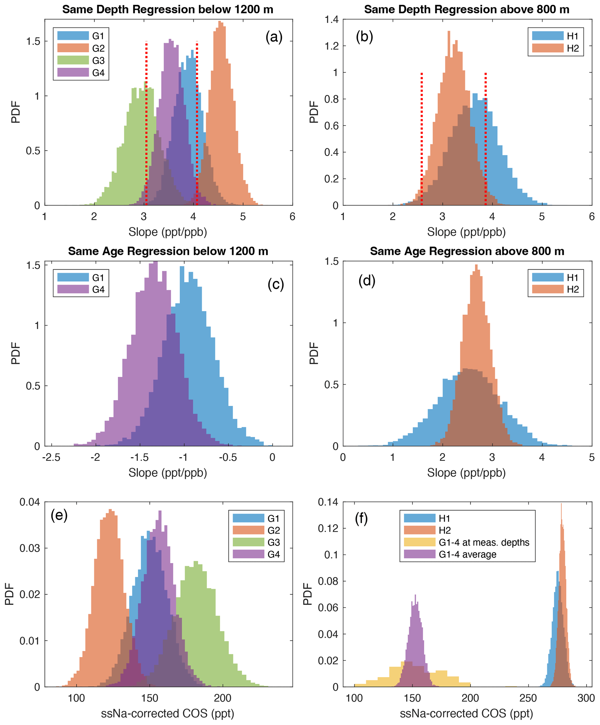
Figure 3(a) PDFs of the same-depth errors-in-variables regressions for the glacial period (below 1200 m) dry-extraction COS measurements under four different analysis scenarios (Sect. 3.1). (b) The same as (a) but for the two Holocene (above 800 m) scenarios. In (a) and (b), the ±2σ (95 %) confidence intervals (dashed red lines) for the G4 and H2 regressions are shown to demonstrate the high statistical significance (being different from zero) of the PDFs for all scenarios. Panels (c) and (d) are the same as (a) and (b) but for the same-age errors-in-variables linear regressions. (e) Distributions of all dry COS measurements from 52–23 ka after correction with ssNa under G1 through G4 scenarios. (f) Distributions of dry COS measurements after correction with ssNa under H1 (blue) and H2 (red) scenarios. For comparison, distributions of the average across G1 through G4 (purple, n=8000) and the average of all scenarios at discrete depths (yellow, n=177) are also shown. During the LGM, the ssNa-corrected wet COS measurements reach lower levels than what is displayed here for the 52–23 ka period (Fig. 4b).
In subsequent analysis, we find significant correlations between COS and ssNa in the enclosing ice above 800 m (Holocene ice), providing compelling evidence for COS production regardless of the average ssNa concentrations across glacial to interglacial periods (Figs. 2c, d, A5, and A7). The fact that the same-depth relationship between ssNa and COS is stronger when ssNa is averaged over 100 years or more implies that the higher frequency variance in COS is not explained by ssNa variance at similar frequencies (Figs. 1b, A4, and A5). As noted above, the presence of spikes is a contributing factor to the low R2 of the correlations despite the high significance, and we later show that the spikes in the COS signal do not significantly impact the quantification of the relationship with ssNa by smoothing both the COS and ssNa signals in different analysis scenarios (e.g., G2 described in Sect. 3.1). We find no evidence in the soluble ions and dust records that correlate with the spikes evident in the pre-16 ka COS measurements, and the SPC14 record does not display a downcore-increasing trend or a downcore increase in the magnitude of the COS spikes. These observations suggest ssNa is a proxy for a production process confined primarily to the firn column. If some level of additional production happens in the ice sheet after lock-in or in the lab during extraction, which are the types of processes that can result in sharp spikes, the high-frequency variations in bulk measures of marine (ssNa) or terrestrial (nssCa) aerosols are not good proxies for it.
We considered the possibility of the correlation with ssNa arising from a climate-driven relationship between ssNa and COS that somehow influences the same-depth regressions; however, during the glacial period the difference between ice age and gas age (delta-age) for the SPC14 ice core is large and temporally variable (Fig. A1b), implying this is unlikely. Indeed, same-age correlation analyses display a negative correlation during the glacial period, ruling out the possibility of a climate-driven relationship as the explanation for the positive same-depth relationships (Figs. 3c and A6). The same-age analysis reveals a positive relationship during the Holocene, but this does not negate the same-depth relationship (Figs. 3d and A7). Rather, simultaneous regressions of COS vs. same-depth and same-age ssNa (Sect. 2.4) confirm that two independent relationships exist between ssNa and COS, the same-depth one, which is driven by production, and the same-age one that can be interpreted as a climate-mediated variability in the ice core COS record.
3.1 Results of different analysis scenarios: inferred atmospheric COS variability after the ssNa correction
The results from all of the analysis scenarios yield similar estimates of atmospheric COS variability after correction for the presence of excess COS in the ice core measurements (Fig. 4b). In G1, the errors-in-variables slope of the 100-year ssNa vs. COS same-depth regression is used to correct the COS record (Figs. 2–4 and A5a–c). This scenario does not include any smoothing of the COS measurements, which leads to a relatively low R2 partially because high-frequency variability in COS (the spikes) do not correlate with ssNa. In G2 (Fig. A5d–f), we smooth the COS measurements with a seven-point moving average, which approximates to an 1143-year averaging window, and use the seven-point moving standard error of the measurements themselves as the y-variable error in place of the original measurement errors. The ssNa measurements are also smoothed to 1100 years to match COS. Collectively, these choices lower the influence of the COS spikes from the regression via smoothing and introduce higher uncertainty to the y-variable COS where there is a higher occurrence of COS spikes. The R2 for G2 (0.22) is significantly higher, whereas the mean slope estimate increases marginally, indicating the same-depth ssNa–COS relationship is driven primarily by millennial-scale variability and is not influenced by the higher-frequency COS spikes.
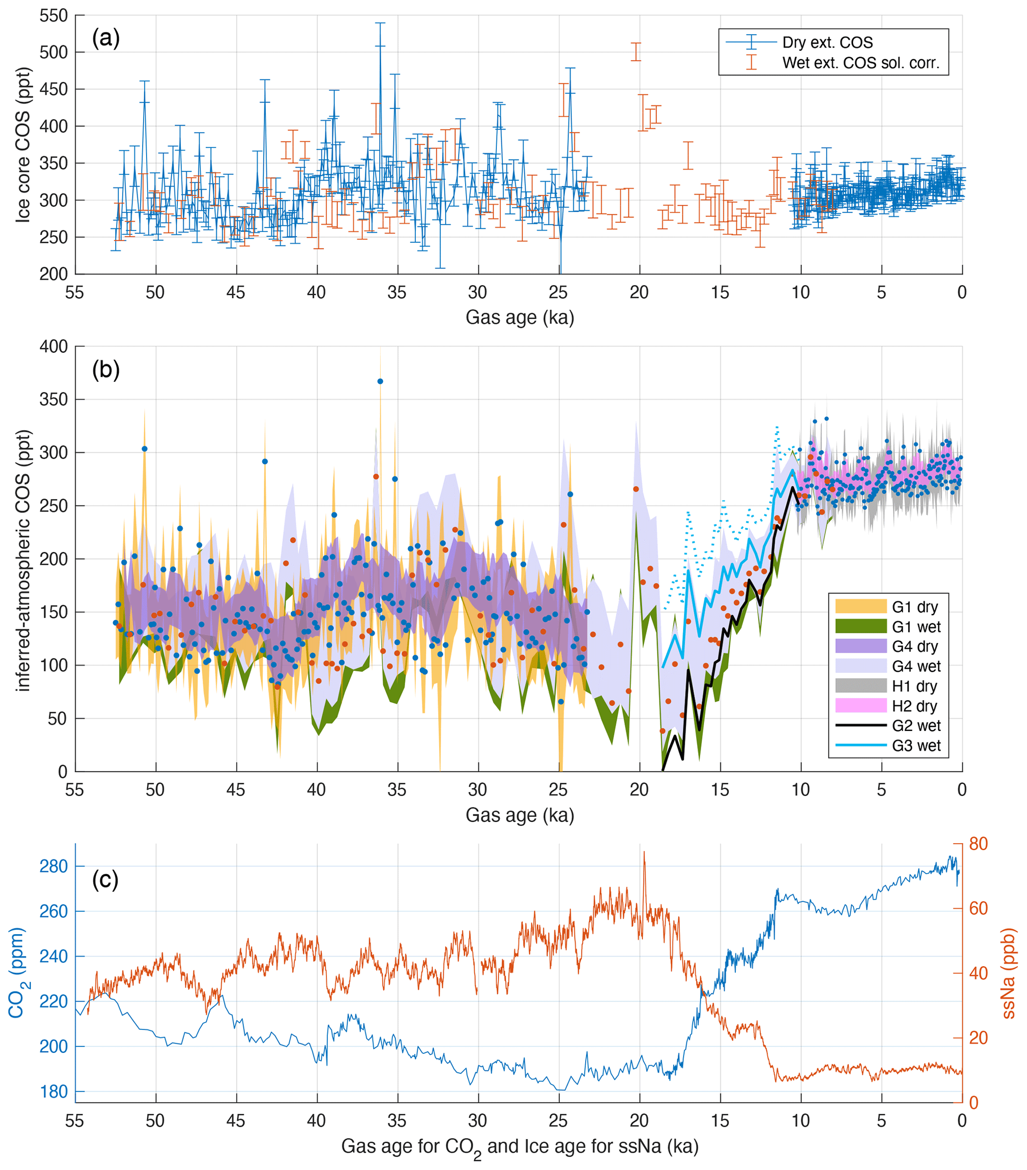
Figure 4(a) The SPC14 COS measurements from Fig. 1a with ±1σ measurement errors. (b) The inferred (ssNa-corrected) atmospheric COS record. The filled markers denote the individual data points corrected with G1 and H1 scenarios for the dry measurements (blue) and G1 for the wet measurements (red). The colored bands (see legend) denote posterior ±2σ ranges (Sect. 2.4) for all analysis scenarios shown in Fig. 3a–d; the full PDFs for G1 through G4 and H1 and H2 scenarios are shown in Fig. 3e and f. The wet G1±2σ range is mostly masked by the wet G4±2σ range. For clarity, only the posterior means (lines) through the deglaciation are shown for the wet G2 and G3. The dashed blue line is the +2σ range for the G3 scenario, representing an upper limit (albeit one with very low probability). (c) A composite Antarctic ice core CO2 record (blue – left y axis) and the 100-year smooth ssNa record from the SPC14 ice core (red – right y axis) vs. gas age and ice age, respectively (Bereiter et al., 2015; Winski et al., 2021).
The analysis scenario G3 (Fig. A5g–i) differs from G2 primarily in that we reduce the weight of COS spikes on the regression by smoothing the COS record by a seven-point moving median. The treatment of y-variable errors also changes. We use a seven-point root mean square of the original COS measurement errors and introduce a constant multiplier (α in Eq. 8) to allow the Bayesian inference to scale the y errors as needed (Sect. 2.4). The G3 scenario demonstrates the impact of minimizing the influence of COS measurement uncertainties on the errors-in-variables analysis as the y-variable errors in G3 are more uniform by design and are scaled up by more than a factor of 3 via the α parameter (Fig. A5l), resulting in a closer slope estimate to the least squares linear regression of the data used in the G3 scenario (compare slopes in Fig. A5g vs. G3 in Fig. A5i).
In G4 (Figs. A5j–l and A6f–i), we introduce a simultaneous same-age regression of COS with ssNa. As noted earlier, the same-age correlation between COS and ssNa is interpreted as a climate-driven relationship. The delta age is 1500–2700 years over the 1200–1751 m depth range (Fig. A1b) corresponding to 30–54 m of ice for an average annual-layer thickness of 2 cm, implying only multi-millennial-scale climate trends would have an impact on accurate quantification of the same-depth slope. We also conduct an independent same-age-only regression of measured COS vs. 100-year smooth ssNa (Fig. A6a–c, same-age regression for G1). The same-age regression slopes for G1 and G4 have mostly overlapping PDFs and similar means (Fig. 3c), revealing a climate-driven negative correlation between ssNa and COS over multi-millennial timescales that impacts accurate quantification of the slope of the same-depth relationship (Fig. A5i). Detrending COS with the same-age ssNa–COS relationship increases the R2 of the same-depth regression to 33 % (Figs. 2c and A5j). The G4 results are a more accurate estimate of the same-depth slope than G3 as it implicitly accounts for the influence of the climate-driven variance in the record while quantifying the same-depth relationship between ssNa and COS.
We conducted two similar data analysis scenarios (H1 and H2) for the dry-extraction measurements from above 800 m. In H1 (Fig. A7a–c and g–i), the same-depth and same-age correlations are identified independently using COS measurements (49-year resolution on average) and 100-year smooth ssNa. In H2 (Fig. A7d–f and j–l), we apply a seven-point smoothing to the COS record (350-year smoothing window on average) and conduct simultaneous same-depth and same-age regressions vs. 300-year smooth ssNa. We find significant positive correlations between ssNa and COS from the same depth and from the same age. Quantification of the same-age relationship with the simultaneous regression does not significantly change the mean slope of the same-depth relationship but results in a narrower probability distribution, and hence it increases its significance (Fig. A7c and f). The results of the different scenarios display the most likely range of atmospheric COS variability over the last 52 000 years with the 2σ uncertainty ranges representing ±2 SD of the posterior probability distributions from the different scenarios (Fig. 4b).
Collectively, the different analysis scenarios yield comparable estimates for average COS levels over long timescales and all imply lower atmospheric COS during the last glacial period (Fig. 4b). The inferred atmospheric record averages about 150 ppt from 52.5 to 25 ka, which is more than 100 ppt lower than the Holocene mean (Fig. 3f). During the late Last Glacial Maximum (LGM) around 18 ka, the probable range for atmospheric COS falls below 100 ppt, after which atmospheric levels rise through the deglaciation to reach 250–300 ppt during the Holocene. Note that at 18 ka, atmospheric COS is more likely to be less than 50 ppt than higher than 100 ppt, and 150 ppt is the upper limit for this period.
We conducted additional analyses to test the sensitivity of results from the different scenarios to (1) minor depth offsets to the ssNa data used in the regressions and (2) elimination of some fraction of the data from the regressions. We find that the best correlations are achieved when COS is regressed vs. ssNa from the same depth and that the results are repeatable at lower data densities but that significance gets progressively worse with less data (Appendix B). Next, we tested the robustness of the same-age relationship between ssNa and COS with respect to the applied same-depth correction and found that the temporal relationship with ssNa during the glacial period is likely inherent to the COS data set and does not result from the applied same-depth ssNa correction (Appendix C). Finally, we also tested whether there is any explicit statistical evidence that the increase in the inferred atmospheric COS record concurrent with the deglaciation during 19–10 ka is climate driven as opposed resulting solely from the applied ssNa correction. We find that the deglacial increase in atmospheric signal is more similar to the deglacial climate signal than the inverse of the applied ssNa correction (Appendix D).
3.2 Comparison of the SPC14 record with records from other Antarctic ice cores
Comparison of the SPC14 record to previous ice core measurements is challenging. There is no other COS data set that does not require a hydrolysis loss correction (i.e., no data from another very cold site) or that is at a comparable resolution to the SPC14 record from the glacial period that would allow an investigation of impurity-driven COS production impacting the measurements. We presume that some COS production occurs at every site and that this is the reason why the WD and TD records trend in different directions during the late deglaciation even after the hydrolysis loss correction. Subsections of the COS measurements from the TD and WD sites do not require large corrections for the hydrolysis loss due to relatively cold temperature histories: during the glacial period at WD and during mid-to-late Holocene at TD. We make use of this fact to conduct a preliminary analysis to determine whether a same-depth relationship exists between ssNa and COS at these sites during these periods.
The same-depth relationships between ssNa and COS in TD during the Holocene and WD during the glacial period and deglaciation are similar to the SPC14 observations (Fig. A11). Given the impact of lower data density on regressions (Sect. 3.2), instead of determining site-specific correction slopes, we correct the TD and WD measurements using the G4 correction slope estimate from the SPC14 ice core (Fig. 5). The COS production occurs primarily in the firn, whereas hydrolysis loss is a slow process occurring over multi-millennial timescales (Aydin et al., 2014, 2016). Therefore, the ssNa correction is applied to the loss-corrected COS records. This comparison is considered preliminary and evaluated qualitatively given that the general applicability of the same-depth ssNa–COS regression slopes has not been tested.
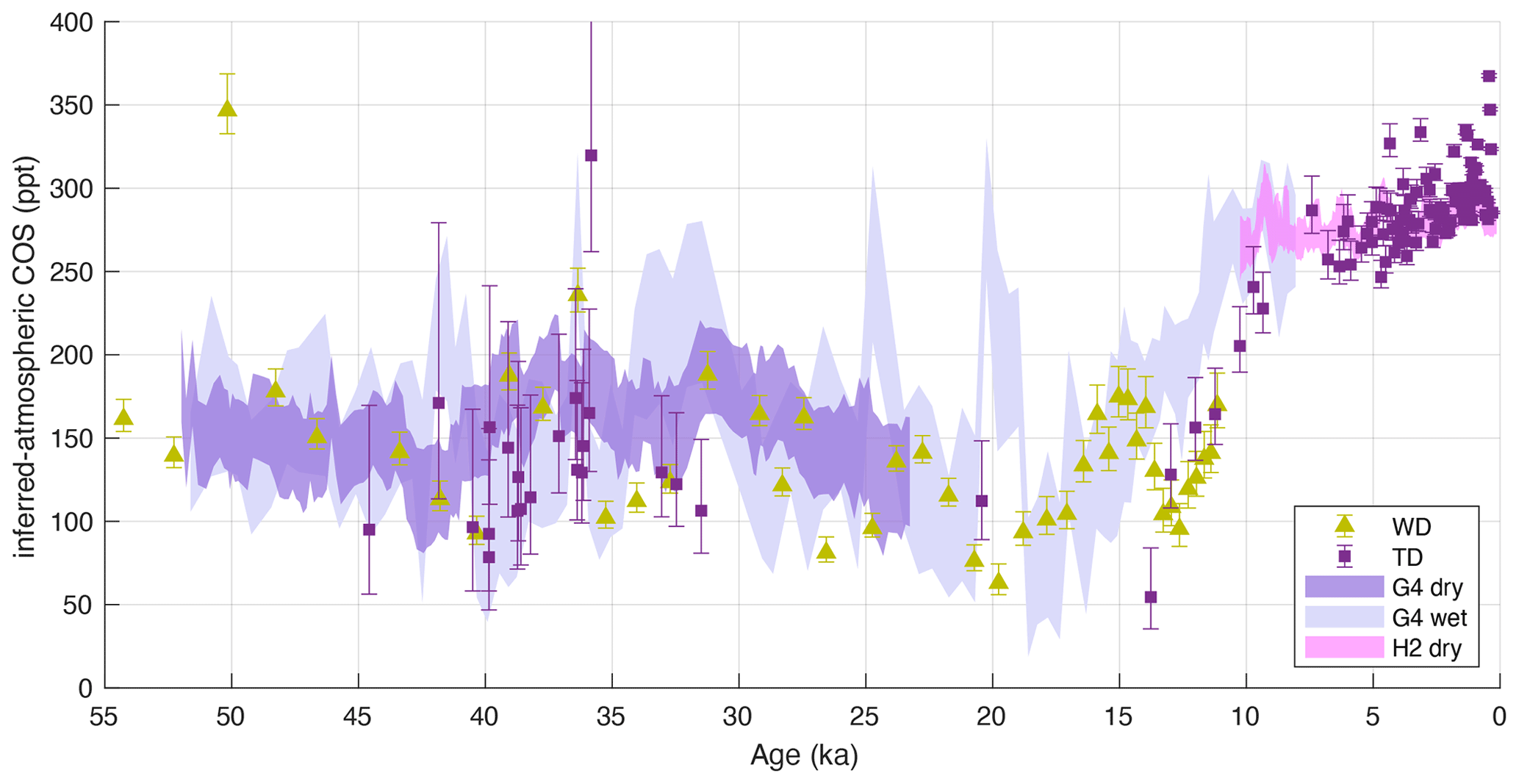
Figure 5The ice core COS records from the TD (purple squares) and WD (green squares) ice cores are corrected for COS production using the G4 ssNa–COS errors-in-variables regression slope. The ssNa-corrected South Pole record for different scenarios (Fig. 4b) is shown in the background.
After the ssNa correction, the Taylor Dome record agrees better with the SPC14 record during the glacial period from 45–20 ka and also suggests a steep increase during the deglaciation similar to the SPC14 record (Fig. 5). The timing of the deglacial COS increase is somewhat different for the Taylor Dome record vs. the SPC14 record. The discrepancies could result from the use of constant and SPC14-specific ssNa correction parameters, but there may be other contributing factors. The full range of uncertainty in the Taylor Dome loss correction arising from the uncertainties in the temperature histories have not been quantified (Aydin et al., 2014, 2016). Further, the Taylor Dome chronology during the LGM and the deglaciation is susceptible to larger uncertainties than the SPC14 ice core, including known errors during the early Holocene because the current Taylor Dome gas chronology is tied to the outdated EDC-1 chronology (Monnin et al., 2004). Chronology errors impact the hydrolysis loss correction too as this correction is both temperature and time dependent.
The ssNa-corrected WDC-06A record agrees better with the SPC14 record during the glacial period and through 14 ka, capturing the first few thousand years of the COS rise during the glacial–interglacial transition (Fig. 5). However, the WDC-06A record does not show any indication of a peak near 19 ka. The WDC-06A record also displays a deep trough around 13 ka. The relative age uncertainty between the SPC14 and WD ice cores is 100 years or less for most of the core (Epifanio et al., 2020). At least part of the discrepancy between the three ice cores during the late deglaciation might be due to the fact that the SPC14 ssNa correction parameters are not broadly applicable to the Taylor Dome and WAIS Divide ice cores during these periods. The other contributing factor could be the unquantified uncertainties in the hydrolysis loss corrections applied to the WDC-06A and Taylor Dome records.
4.1 COS production in the ice sheet
Production of trace gases can occur both in the firn and in deeper ice below bubble lock-in presumably from ice impurities (Butler et al., 1999; Fain et al., 2014; Mühl et al., 2023). If the excess gas amount is comparable to the mean atmospheric levels, a correlation between the gas and the ice impurities would start to emerge. If production starts immediately below bubble close-off and stops after a relatively short period, the excess gas would correlate with the impurity concentrations measured over the exact same depth range as the gas sample. This scenario is conceptually unrealistic because there is no obvious reason why there would not be a firn component to any production process that takes place in the ice sheet, with the only exception being production in very deep, warm, and wet ice possibly with incorporated bedrock material. It could be reasonable to ignore the firn component if the production continues over much longer time horizons than the firnification timescale. If this is case, the continual accumulation of excess gas over time should introduce a long-term increasing trend to the gas record that would be absent from the impurity record underlying the production. In contrast, if the trace gas production is short-lived, production in the firn could be the primary component, in which case the excess gas is expected to correlate with the impurities but over a larger depth range than the exact length of the ice core samples because of vertical mixing of gases in the firn.
The relationship between the SPC14 COS measurements and ssNa favors a process primarily taking place in the firn because there is no long-term trend in excess COS (i.e., production is a relatively short-lived process) and the correlation with ssNa is driven by longer time periods than the age range that corresponds to the length of our samples. In theory, it is also possible gas production can happen in the laboratory during the extraction of the ice core air. We deem this unlikely because production during extraction should also result in a correlation with impurities measured over the exact same depth range as our samples. Further, the agreement between COS measurements with two different extraction methods implies excess COS is generated in the ice sheet. The production process may be short-lived because reaction substrates run out over time, lowering the probability of reactions as the ice ages. Further, solid- and dissolved-phase ice impurities, e.g., sea salt aerosols and trace metals that can act as reaction substrates and catalysts for production of COS, can migrate to different locations via post-depositional processes that occur in shallow ice (Stoll et al., 2023), also lowering the probability of complex reactions deeper in the ice sheet.
To demonstrate the viability of the proposed production process as an explanation for our observations, COS production in the firn is simulated within an advective–diffusive model of the South Pole firn (Aydin et al., 2020). The model tracks a layer of impurity (e.g., ssNa) that induces gas production (e.g., COS) at a fixed rate (1 ppt yr−1) through its progression in the firn from the surface to the bottom (Fig. 6). In this framework, the excess gas peak at any given depth in the firn is always broader than the production peak in both directions (up and down the firn) because as soon as the gas is produced, it starts to mix vertically. The model also demonstrates that the excess gas produced in the lock-in zone (below 100 m at the South Pole) accumulates with much higher efficiency, resulting in progressively sharper peaks with depth. Another important implication is that the R2 statistic between the excess gas and the impurity concentration at the same depth is considerably less than 1 even in the absence of any underlying atmospheric variability or measurement uncertainty (Fig. 6).
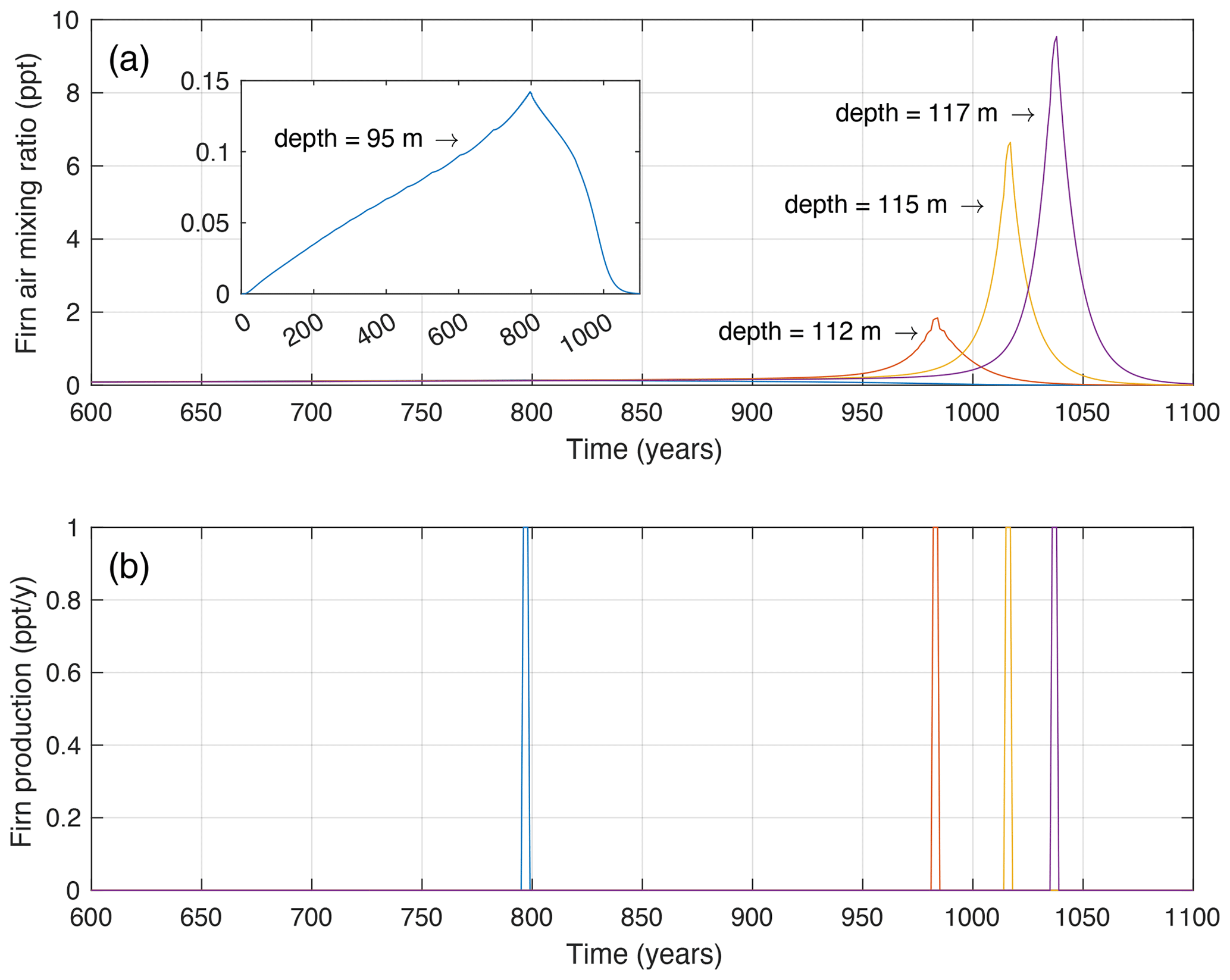
Figure 6Modeled trace gas production in the South Pole firn from an impurity layer. (a) Firn air trace gas mixing ratio (y axis) vs. time (x axis) at 95 m (blue), 112 m (red), 115 m (yellow), and 117 m (purple). The 95 m profile is shown in the inset because the excess gas peak at this depth is not visible at the scaling of the parent plot. Note that the gas mixing ratio at any given depth peaks when the production occurs at that depth. (b) Gas production vs. time at the same depths as (a).
In the absence of direct empirical evidence, we can only speculate on viable mechanisms for the COS production in the firn. The ssNa data approximate marine aerosol deposition to the ice sheet (Winski et al., 2021). It follows that the COS production mechanisms might be similar to the dark production mechanisms in the ocean. We focus on dark production because the photochemically active zone in an ice sheet is largely constrained to the top meter of the firn (Grannas et al., 2007; King and Simpson, 2001), and our model simulation shows that only a tiny fraction of the gases produced in shallow firn can be preserved in the ice sheet (Fig. 6). There is not a well-established mechanistic explanation for dark production of COS in the ocean (Cutter et al., 2004; Von Hobe et al., 2001), but recent studies favor chemical mechanisms over biological ones (Lennartz et al., 2017, 2019). The commonly postulated abiotic process involves reactions between carbonyl groups and thiyl radicals derived from organic sulfur (Flöck et al., 1997; Modiri Gharehveran and Shah, 2018; Lennartz et al., 2017, 2019; Pos et al., 1998; Zepp and Andreae, 1994). Organic salts have been used as carbonyl donors for COS production in laboratory settings (Pos et al., 1998). Sea salt aerosols host a variety of chemical reactions during atmospheric aging, including reactions between NaCl and organic acids leading to production of organic salts of Na (Laskin et al., 2012). This could explain why ssNa works as a proxy for excess COS. Abiotic COS production also requires an organic sulfur source. Antarctica is far from continental land masses, suggesting marine aerosols could also be the primary source of organic sulfur. Reactions between organic salts and sulfur can be catalyzed in the dark by transition metals (Modiri Gharehveran and Shah, 2018; Lennartz et al., 2019; Pos et al., 1998).
4.2 Interpretation of the atmospheric COS record
The ssNa correction is relatively small during the Holocene (Fig. A1c) and implies 10 %–15 % less COS in the preindustrial atmosphere than what was previously inferred from uncorrected measurements (Aydin et al., 2020). Excess COS of this magnitude is difficult to identify with firn measurements because of the uncertainties involved in the firn measurements and inversions. There is a positive same-age correlation between ssNa and COS during the Holocene that arises primarily from the dip centered around 6 ka in both records and to a lesser extent a subsequent long-term rise followed by a decrease over the most recent 700 years (Fig. A7k). The ssNa variability apparent in the SPC14 ice core during the Holocene tracks winter sea ice extent in the Southern Ocean (Winski et al., 2021). Modern-day winter sea ice concentrations around Antarctica have been linked to organic acid emissions from phytoplankton blooms, which also emit DMS (Curran and Jones, 2000; King et al., 2019). Direct COS fluxes are also high in the Southern Ocean but have not been linked to sea ice (Kettle et al., 2002; Lennartz et al., 2017, 2019). It is possible that atmospheric COS is sensitive to changes in ocean DMS emissions modulated by winter sea ice. Further research is needed on whether COS is co-emitted with DMS along the sea ice margins.
During 52–25 ka, the 2σ confidence interval of G4 mostly remains between 100–200 ppt, averaging about 150 ppt (Fig. 4c), which is lower than the mean levels during the Holocene by about a factor of 2 (Fig. 3f). This difference is quantified directly by the dry measurements and is highly significant. During the LGM minimum delineated by the wet measurements, the probable range of atmospheric COS is less than 100 ppt, implying a rise by a factor of 3–4 concurrent with the deglaciation. In Sect. 3.3, we show that the same-age anticorrelation with ssNa is evident even in the regression of measured COS with ssNa (Fig. 3c) and not caused by the same-depth correction. The analysis in Sect. 3.4 provides strong statistical evidence that the temporal evolution of the deglacial COS arises from the variability inherent to the COS measurements. The deep COS minimum at the end of the LGM appears to result from the culmination of a long-term trend that starts prior to 30 ka and is climate driven.
Shorter-period temporal variability apparent during the glacial period requires additional scrutiny. The methods we use in applying the ssNa correction do not explicitly address the possibility of temporal variability in the ssNa correction slope. Therefore, the actual temporal trends in atmospheric COS may not track the mean of the posteriors for any of the analysis scenarios. However, the reported ±2σ uncertainty ranges are determined by correcting the COS measurements with a range of slope values drawn from the posterior PDFs (Fig. 3a and b) while also accounting for measurement uncertainties. If the same-depth ssNa–COS relationship varies over time but stays within the range of the slope PDFs, the inferred COS variability should remain within the reported uncertainty ranges, particularly over long timescales. Temporal variability in the correction slopes that exceed the posterior ranges of the different scenarios cannot be ruled out; however, such temporal variability could only last for brief periods such that it would not alter the long-term mean states described by the slope posteriors. In the remainder of this section, we will primarily focus on the interpretation of the deglacial increase in mean COS levels. We do not offer a biogeochemical explanation for the COS spikes because it is unlikely that they represent atmospheric variations, with the possible exception of the sharp peak around 19 ka.
The 19 ka peak is characterized by four wet COS measurements and coincides in time with a shorter-lived sharp peak in ssNa (Fig. 4c). Given the prominence of spikes in the glacial period COS, we suspect that at least one of the measurements characterizing the 19 ka COS peak, possibly the highest measurement dating older than 20 ka, may be a coincidental, non-atmospheric spike, while the other three measurements may characterize an atmospheric excursion of 50–100 ppt that is closer in duration to the peak in ssNa. This may explain why we do not see this feature in the WD COS record. An atmospheric COS excursion of this magnitude would represent a sudden and significant departure from the biogeochemical balance that maintains the low atmospheric COS levels during the LGM. Based solely on the magnitude, it could only be caused by an increase in ocean sulfur gas emissions or a decline in land biosphere uptake since these are the two major natural components of the COS budget (Table 1). This feature warrants further investigation if replicated with high-resolution measurements from different ice cores.
The 2–4-fold increase in atmospheric COS across the deglaciation implies equivalent changes in the sources or the removal processes. The atmospheric lifetime of COS is linked to the gross primary productivity (GPP) of land plants, atmospheric carbon dioxide (CO2) levels, and the leaf-scale relative uptake (LRU) of COS vs. CO2 (Stimler et al., 2010). CO2 is relevant because the first-order loss rate constant for atmospheric COS via plant uptake (kveg) is proportional to stomatal conductance, which is inversely proportional to CO2 (Stimler et al., 2010):
In Eq. (11), a change in atmospheric CO2 results in a proportional change in the COS lifetime if GPP and LRU are constant. Atmospheric CO2 increases from 190 to 270 ppm (factor of 1.4) during the deglaciation (Fig. 4c), which implies an equivalent increase in the COS lifetime.
Of course many large-scale changes in the terrestrial biosphere occur during the deglaciation, and it is unlikely that GPP and LRU remain constant. The warmer interglacial world has less ice sheet cover and more CO2 in the atmosphere, promoting a general expansion of plant coverage that favors woody plants (C3) over grasslands (C4) and an increase in GPP by 40 %–50 % (Ciais et al., 2012; Prentice et al., 2011). The effect of increasing GPP is equivalent to but in the opposite direction of the CO2 effect on the COS lifetime. LRU varies with light, humidity, and CO2, but these effects are small for realistic ranges of change in global average conditions (Sun et al., 2022). LRU is relatively more sensitive to photosynthetic pathways and is higher for C3 plants than C4 plants (Stimler et al., 2011; Sun et al., 2022), suggesting this effect would dominate the LRU response to the deglaciation and result in a shorter lifetime during the Holocene. Since the other loss processes are too small (Table 1), we presume that all or most of the COS rise during the deglaciation is driven by emissions and has to involve all major sources since the required increase is very large. If the COS lifetime were shorter during the Holocene, the proportional increase in emissions during the deglaciation would have to be higher than the increase apparent in the COS mixing ratio.
Biomass burning likely increased during the deglaciation (Bock et al., 2017); the anoxic sources would also have to increase if their emissions are closer to the upper limit of estimates. Still, oceans are the largest COS source, and most of the required increase must come from the combined emissions of COS, CS2, and DMS (Berry et al., 2013; Glatthor et al., 2015; Kettle et al., 2002; Kuai et al., 2015; Lennartz et al., 2017; Ma et al., 2021; Whelan et al., 2018). Photochemical production mediated by chromophoric dissolved organic matter (CDOM) is the primary production mechanism of COS in the surface ocean, with an additional dark (light-independent) channel (Flöck et al., 1997; Modiri Gharehveran and Shah, 2018; Lennartz et al., 2017, 2019; Von Hobe et al., 2001; Zepp and Andreae, 1994). COS is chemically lost to temperature-dependent hydrolysis in the surface ocean, and emissions occur primarily in temperate waters and higher latitudes where hydrolysis is slow (Berry et al., 2013; Kettle et al., 2002; Lennartz et al., 2017; Whelan et al., 2018). Low-latitude emissions of COS are predominantly in coastal waters and upwelling regions where CDOM concentrations are high (Kettle et al., 2002; Lennartz et al., 2017, 2019; Nelson and Siegel, 2013; Zepp and Andreae, 1994). The primary CS2 production mechanisms are photochemical, much like COS but possibly involve a different class of organosulfurs that correlate with dissolved organic sulfur in the water; dark production and production by phytoplankton are also possible. CS2 emissions occur primarily in the low latitudes as chemical loss rates are negligibly slow even in warm waters (Kettle et al., 2002; Modiri Gharehveran and Shah, 2018; Lennartz et al., 2017, 2019, 2020; Xie and Moore, 1999). DMS is produced from dimethylsulfoniopropionate (DMSP), a phytoplankton product, and water column losses are due to microbial metabolism and photosensitized oxidation (Andreae, 1990; Charlson et al., 1987; Vogt and Liss, 2009; Wang et al., 2018a). Ocean DMS concentrations are generally high where COS emissions are high, but area-integrated emissions peak at the lower latitudes and mid-latitude Southern Hemisphere where CS2 emissions occur (Lana et al., 2011). DMS is also a weak precursor of COS in seawater (Modiri Gharehveran and Shah, 2018; Zepp and Andreae, 1994), and emissions of all three sulfur gases can be co-located with COS, CS2, and DMS emission enhancements in nutrient-rich coastal seas and upwelling regions (Andreae, 1990; Charlson et al., 1987; Ksionzek et al., 2016; Lana et al., 2011; Lennartz et al., 2017, 2019; Wang et la., 2018a; Whelan et al., 2018; Xie and Moore, 1999). The mechanistic understanding of COS production from atmospheric oxidation of DMS is evolving (Khan et al., 2021; Jernigan et al., 2022), and the upper limit for this indirect source is uncertain (Table 1).
The similar timing of the atmospheric COS and CO2 increases during the deglaciation suggests that COS is responding to global environmental changes driven by climate. Expected temperature and pH changes during the deglaciation may result in weak enhancements in the net oceanic emissions of sulfur gases via impacts on solubility and hydrolysis, but these effects are not on the same order as the apparent COS increase during the deglaciation (Appendix E). High-magnitude emission changes can be caused by increases in the surface ocean concentrations of dissolved organosulfurs and CDOM, which are primarily byproducts of biogenic productivity and microbial degradation of the biomass (Ksionzek et al., 2016; Nelson and Siegel, 2013). Ocean dynamics, sea level rise, and sea ice extent are physical environment variables that can influence biogenic processes and alter ocean sulfur gas emissions.
Much of the excess CO2 in the interglacial atmosphere is attributed to increased upwelling of old carbon from the deep Southern Ocean that also elevates macronutrient and phytoplankton levels around Antarctica (Anderson et al., 2009; Burke and Robinson, 2012; Freeman et al., 2016; Jaccard et al., 2013). Deeper waters are nutrient rich because of remineralization, which also results in higher CDOM in the ocean interior (Nelson and Siegel, 2013). The oceanic mechanisms responsible for the deglacial increase in atmospheric CO2 can enhance DMS emissions via increased phytoplankton biomass and COS emissions by supplying more organic sulfur and CDOM in the Southern Ocean. Decreasing sea ice extent in the Arctic and around Antarctica can further enhance DMS and COS emissions at high latitudes due to increased light availability and air–sea gas exchange (Vogt and Liss, 2009; Wang et al., 2018a, b). Concurrent enhancement of CS2 emissions necessitates activation of processes in the low-latitude oceans such as the proposed productivity increase in the equatorial Pacific induced by upwelling of nutrient-rich waters (Costa et al., 2017; Winckler et al., 2016), which should result in a co-enhancement of DMS emissions. Additionally, the coastal emissions of COS, CS2, and DMS can increase as a response to the deglacial sea level rise and the associated expansion of shelves and coastal seas coupled with increased riverine output of organic matter (Jennerjahn, 2012; Lerman et al., 2011; Peltier and Fairbanks, 2006).
There is paleoclimate evidence for changes in upwelling regimes in both high and low latitudes and changes in process in coastal regions and on continental shelves that can impact ocean emissions of COS, CS2, and DMS during the deglaciation. We cannot quantify how much of the ocean COS source increase results from DMS vs. COS and CS2 because of the complexities of ocean production mechanisms of sulfur gases and the uncertainties in their contribution to the atmospheric COS budget. We suggest that emissions of all three gases are likely to have increased because the geographic distribution of the relatively well quantified ocean sources of atmospheric COS, i.e., direct COS and indirect CS2 emissions, cover most of the global ocean. The net open-ocean emissions of COS and CS2 are geographically decoupled (Lennartz et al., 2020), but open-ocean DMS emissions overlap with net emissions of both gases, and all three gases are emitted at coastal upwelling zones. All ocean sulfur gas emissions ultimately stem from organic life in the ocean, and biogenically driven enhancements of COS and CS2 production in the surface ocean are unlikely to occur without accompanying changes in DMS production in the same direction. Further, when emissions of all three gases increase, relatively small increases are required for emissions of each gas to achieve the same overall change in atmospheric COS. If only COS and DMS or CS2 and DMS increased, i.e., if the emission changes were confined to either the high or the low latitudes, much larger changes in gas emissions would be required within that region to make up for the missing increase from the other region. If the atmospheric COS budget evolves in such a direction that the ocean COS sources are found to be more regional in nature rather than being globally distributed, the deglacial increase in atmospheric COS would consequently imply changes in only those regions of the ocean.
There is independent evidence for a regional enhancement of ocean sulfur gas emissions during the deglacial cycles. A recent interpretation of ice core sulfate data suggests large increases in ocean DMS emissions around Antarctica concurrent with the last seven deglaciations including a doubling during the last deglaciation (Goto-Azuma et al., 2019), which is consistent with our assessment but in disagreement with the earlier interpretations of the ice core sulfur records (Legrand et al., 1991; Wolff et al., 2006). Unlike the ice core sulfate records, atmospheric COS levels over Antarctica are sensitive to global emissions of DMS due to the longer atmospheric lifetime of COS vs. sulfate. DMS emissions in the Southern Ocean alone constitute about 10 % of global DMS emissions (Lana et al., 2011) and are therefore not nearly sufficient to account for the deglacial COS increase.
The climate impacts of COS and DMS are in the same direction and additive, although DMS is by far the more dominant of the two. The radiative forcing expected from a 150 ppt increase in COS is within −0.004 to −0.045 W m−2, with the large uncertainty arising from model discrepancies and uncertainties in the effects of different emission geometries (Brühl et al., 2012; Quaglia et al., 2022; Appendix F). The global net radiative impact of DMS emissions today is estimated at −1.8 to −2 W m−2, with average summertime values over the southern oceans exceeding −9 W m−2 (Thomas et al., 2010; Wang et al., 2018a, b). During the last deglaciation, the total greenhouse gas () forcing was +2.5 to +3.0 W m−2 (Kohler et al., 2017). A doubling of global DMS emissions during the deglaciation could have resulted in global radiative forcing of −1 W m−2, offsetting about a third of the concurrent greenhouse gas forcing, with large regional impacts over the Southern Ocean.
COS measurements from the SPC14 ice core provide evidence for production in the ice sheet that primarily occurs in the firn. The resulting excess COS is a temporally smooth signal, significantly elevating the baseline of measurements from glacial period ice with high impurity concentrations. The measurements also display large spikes (high-frequency variability), which visually dominate the record from the glacial period ice, although their impact on interpretation of the record is not nearly as consequential as the excess COS resulting from production in the firn. The results highlight the importance of evaluating the atmospheric fidelity of trace gas measurements with measurements from glacial period ice with high-impurity content. Firn measurements from different sites may not reveal production in the firn if the excess amount under present-day conditions is small compared with the atmospheric background and should never be considered a good analogue for possible production in the firn during the glacial periods.
We identify ssNa as a proxy for the excess COS in the SPC14 ice core and implement a proxy-based correction method to recover an atmospheric record. It is possible the same approach can be extended to other ice cores, but high-resolution measurements from other sites are necessary to investigate the general applicability of this approach. The atmospheric record inferred from the SPC14 measurements implies higher COS levels during the Holocene than the last glacial period, with a large increase concurrent with the last deglaciation. The deglacial COS rise results from an overall strengthening of atmospheric COS sources, which arguably implies large increases in the emissions of ocean sulfur gases via processes that involve ocean productivity. COS and DMS have direct and indirect climate feedbacks that can impact the evolution of deglacial cycles. Better constraints on the atmospheric COS budget, particularly on the specifics of the ocean sources, coupled with a modeling effort are needed to quantitatively partition the necessary emission increases among different sources and to refine climate implications.
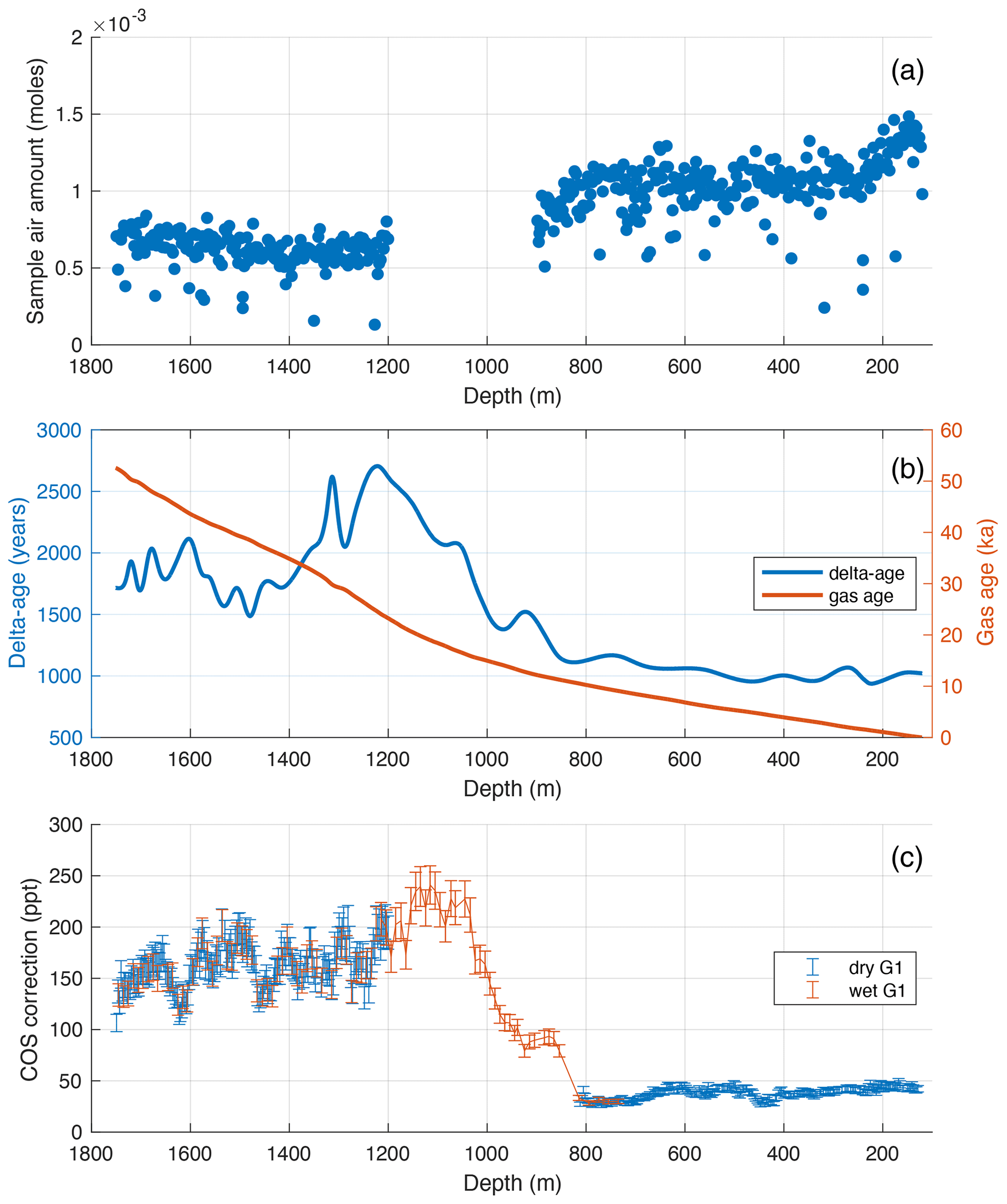
Figure A1(a) Amount of air extracted from the SPC14 ice core samples used for COS analysis with dry extraction. The low outliers are due to smaller ice samples that were commonly half as long. The average amount of air extracted from samples below 1200 m is lower primarily due to a drop in extraction efficiency of dry extraction for full clathrate ice because of the smaller size of clathrates with respect to the bubbles. The presumed bubble–clathrate transition zone from 900 to 1200 m was not analyzed with dry extraction because of expected experimental artifacts. The actual start depth of BCTZ is around 800 m, as evidenced by the downcore decrease in sample air amount. (b) The delta age (left y axis) and gas age (right y axis) for the SPC14 ice core (Epifanio et al., 2020). (c) The correction applied to the COS measurements under the G1 scenario.
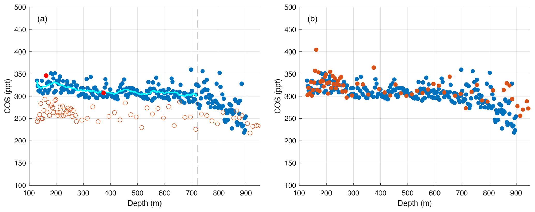
Figure A2The dry-extraction-based (blue) and wet-extraction-based (red) COS measurements from the top 950 m of the SPC14 ice core. (a) The wet-extraction measurements from above 720 m (shallower than the vertical dashed line) are smoothed before being used to determine the solubility correction parameters (Fig. A3). The smooth dry-extraction record (cyan line) is linearly interpolated to wet-extraction measurement depths to estimate COSdry in Eq. (3). Solid red circles denote two outlier wet-extraction measurements that were not included in determination of C3 and C4 in Eq. (3). (b) Solubility-corrected wet-extraction measurements (red) vs. the dry-extraction measurements from (a).
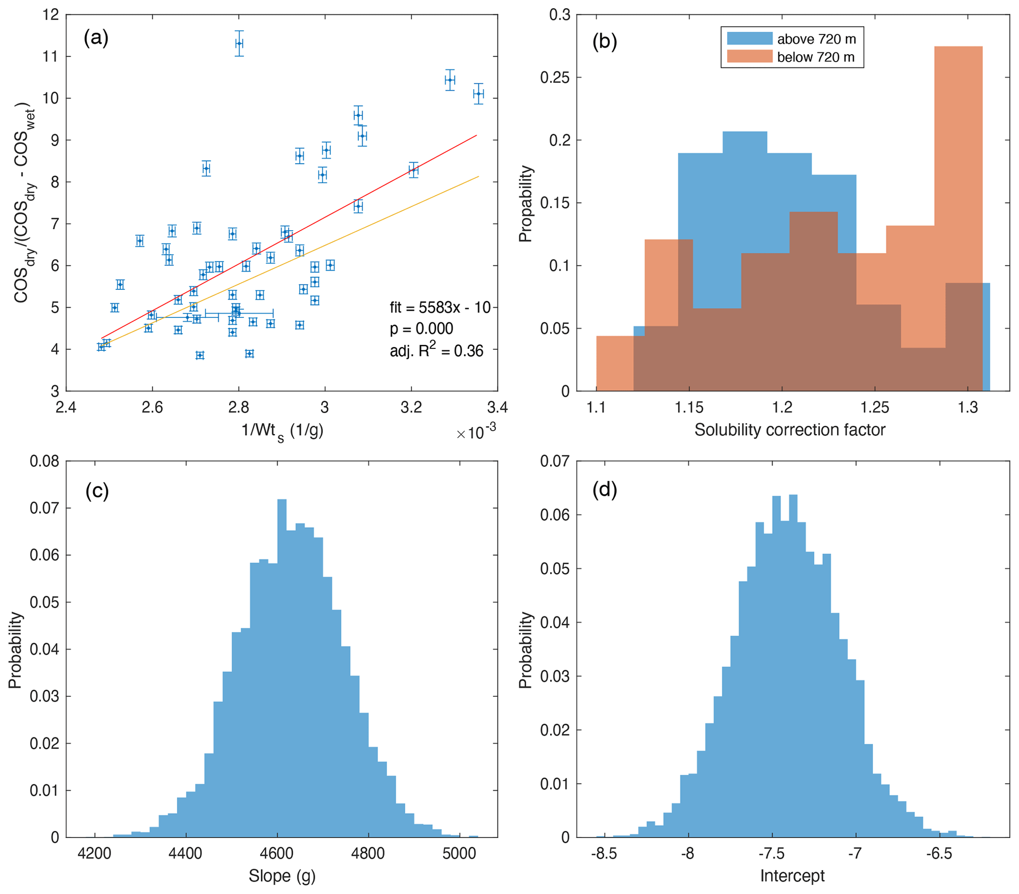
Figure A3Solubility correction parameters and the probability distribution functions (PDFs) of solubility correction factors. (a) Least-squares (red line) and errors-in-variables (yellow line) regressions of Eq. (3). The slope (5583 g) and the intercept (−10 (unitless)) for the least-squares regressions are shown for comparison with the errors-in-variables regression parameters in (c) and (d). (b) The histograms of solubility correction applied to the wet-extraction COS measurements. (c) Probability distribution of errors-in-variables regression. (d) Probability distribution of the intercept of errors-in-variables regression.
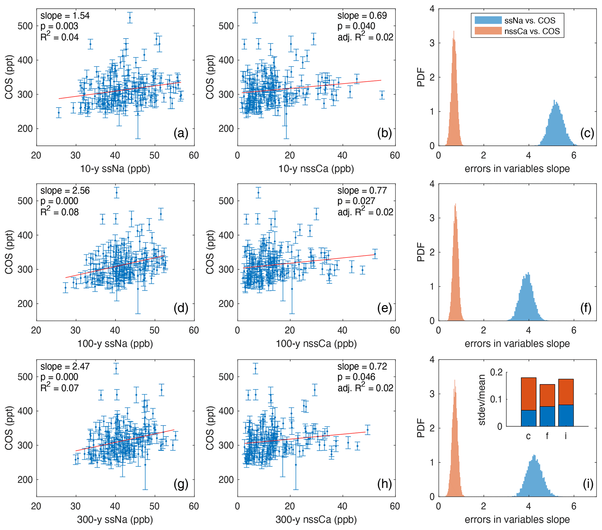
Figure A4Same-depth regression analyses between ssNa and nssCa vs. dry-extraction COS below 1200 m. (a) The 10-year ssNa vs. COS with least-squares regression results. (b) The 10-year nssCa vs. COS with least-squares regression results. (c) Errors-in-variables regression results for (a) and (b). Panel (d) and (e) are the same as (a) and (b) but for 100-year ssNa and nssCa. (f) Errors-in-variables regression results for (d) and (e). Panels (g) and (h) are the same as (a) and (b) but for 300-year ssNa and nssCa. (i) Errors-in-variables regression results for (g) and (h). The inset displays SD mean (a significance metric) for the PDFs shown in (c), (f), and (i).
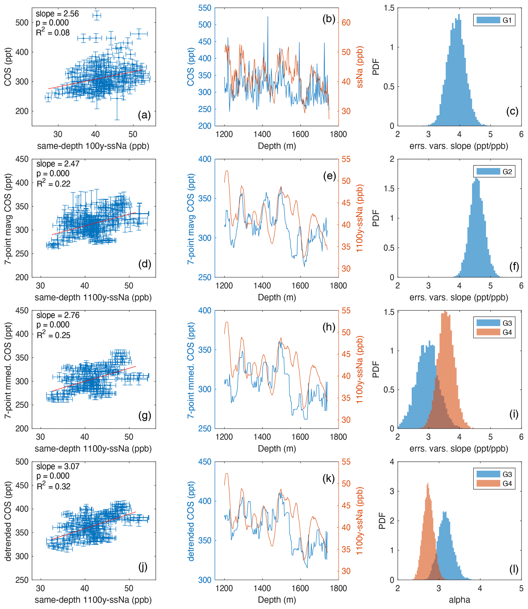
Figure A5Same-depth correlations between ssNa and COS for different glacial period (>1200 m) analysis scenarios. (a) G1 is presented showing the 100-year ssNa vs. COS with least-squares regression results (same as Fig. 2c). (b) Data from (a) vs. depth. (c) Errors-in-variables PDF for (a) (same as in Fig. A4f). (d) G2 is presented showing the 1100-year ssNa vs. seven-point moving average COS with least-squares regression results. (e) Data from (d) vs. depth. (f) Errors-in-variables PDF for (d). (g) G3 is presented showing the 1100-year ssNa vs. seven-point moving median COS with least-squares regression results. (h) Data from (g) vs. depth. (i) Errors-in-variables PDFs for (g) and (j). (j) G4 is presented showing the 1100-year ssNa vs. seven-point moving median COS detrended for same-age correlation with ssNa, shown with least-squares regression results. (k) Data from (j) vs. depth. (l) Errors-in-variables PDFs for the G3 and G4 alpha parameters.
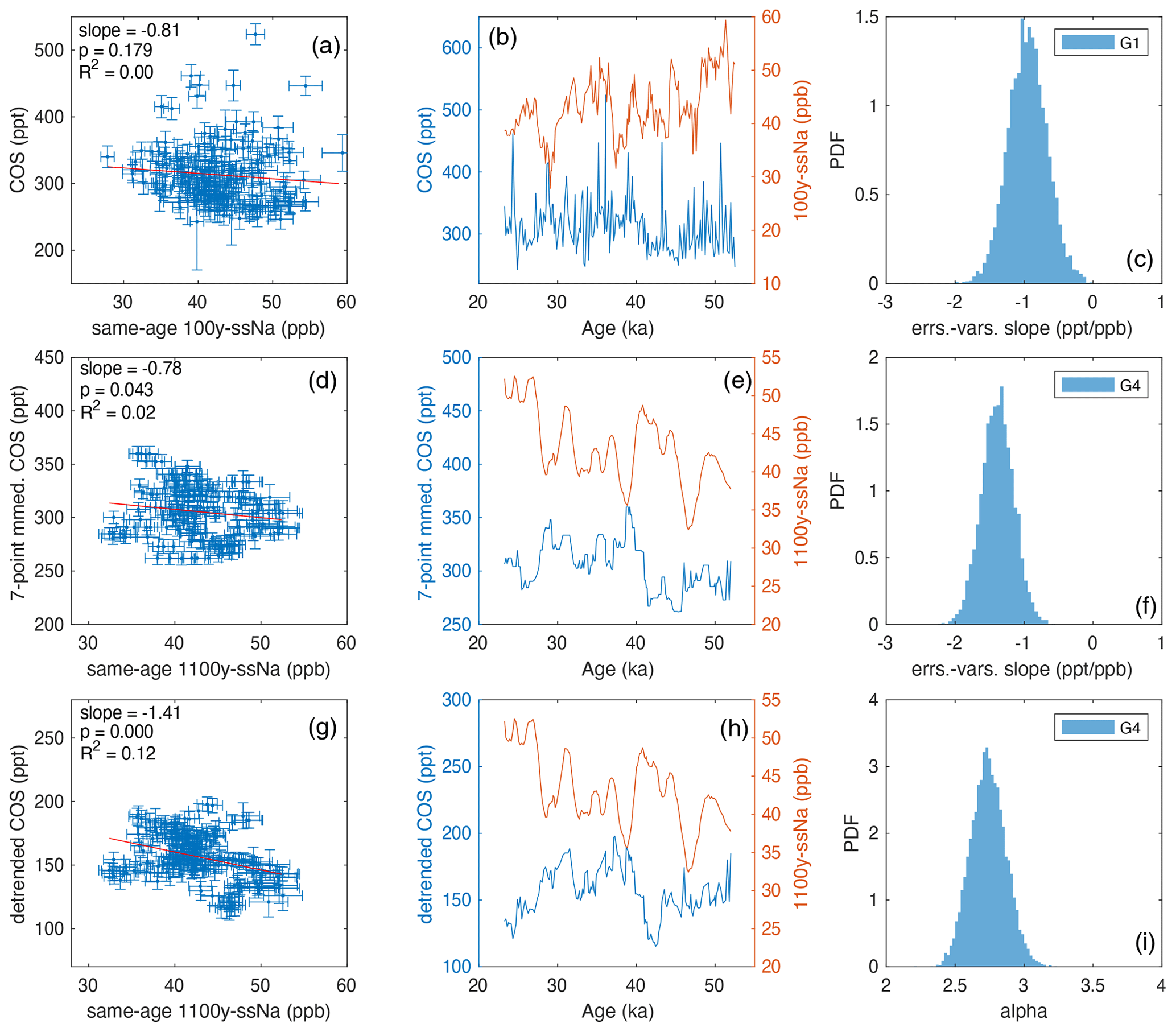
Figure A6Same-age correlations between ssNa and COS for different glacial period (>1200 m) analysis scenarios. (a) Least-squares regression of 100-year ssNa vs. COS. (b) Data from (a) vs. age. (c) G1 is presented showing the errors-in-variables PDF for data shown in (a). (d) Least-squares regression of 1100-year ssNa vs. seven-point moving median COS. (e) Data from (d) vs. age. (f) G4 is presented showing the errors-in-variables PDF for data shown in (g). (g) Least-squares regression of 1100-year ssNa vs. seven-point moving median COS detrended for same-depth correlation. (h) Data from (g) vs. age. (i) Errors-in-variables PDF for the G4 alpha parameter (same as in Fig. A5l).
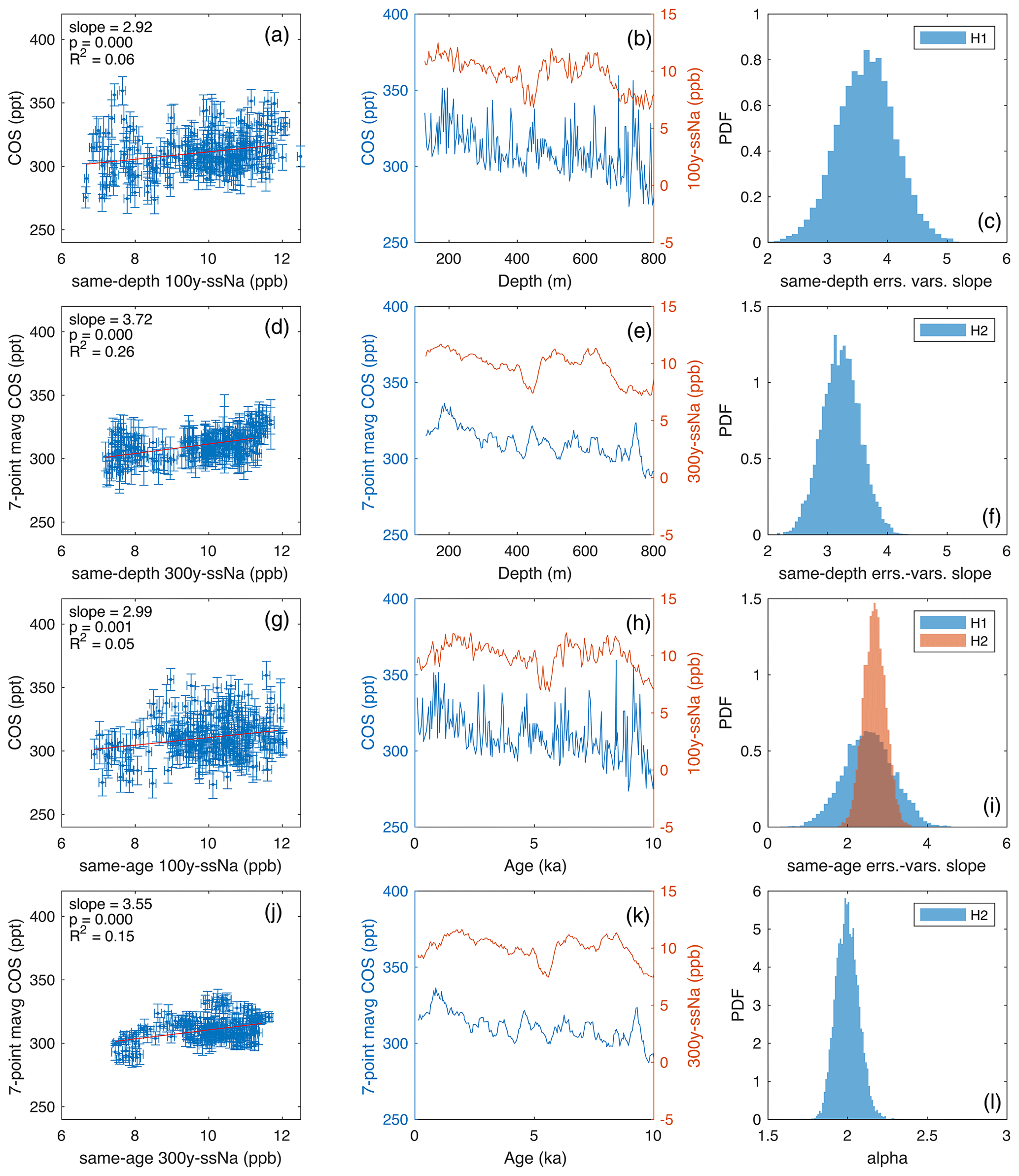
Figure A7Same-depth and same-age correlations between ssNa and COS for different Holocene (<800 m) analysis scenarios. (a) H1 is presented showing the same-depth 100-year ssNa vs. COS with least-squares regression results. (b) The data from (a) vs. depth. (c) Errors-in-variables PDF for (a). (d) H2 is presented showing the same-depth 300-year ssNa vs. seven-point moving average COS with least-squares regression results. (e) The data from (d) vs. depth. (f) Errors-in-variables PDF for (d). (g) H1 is presented showing the same-age 100-year ssNa vs. COS with least-squares regression results. (h) The data from (g) vs. age. (i) Errors-in-variables PDFs for (g) and (j). (j) H2 is presented showing the same-age 300-year ssNa vs. COS with least-squares regression results. (k) The data from (j) vs. age. (l) Errors-in-variables PDF for the H2 alpha parameter.
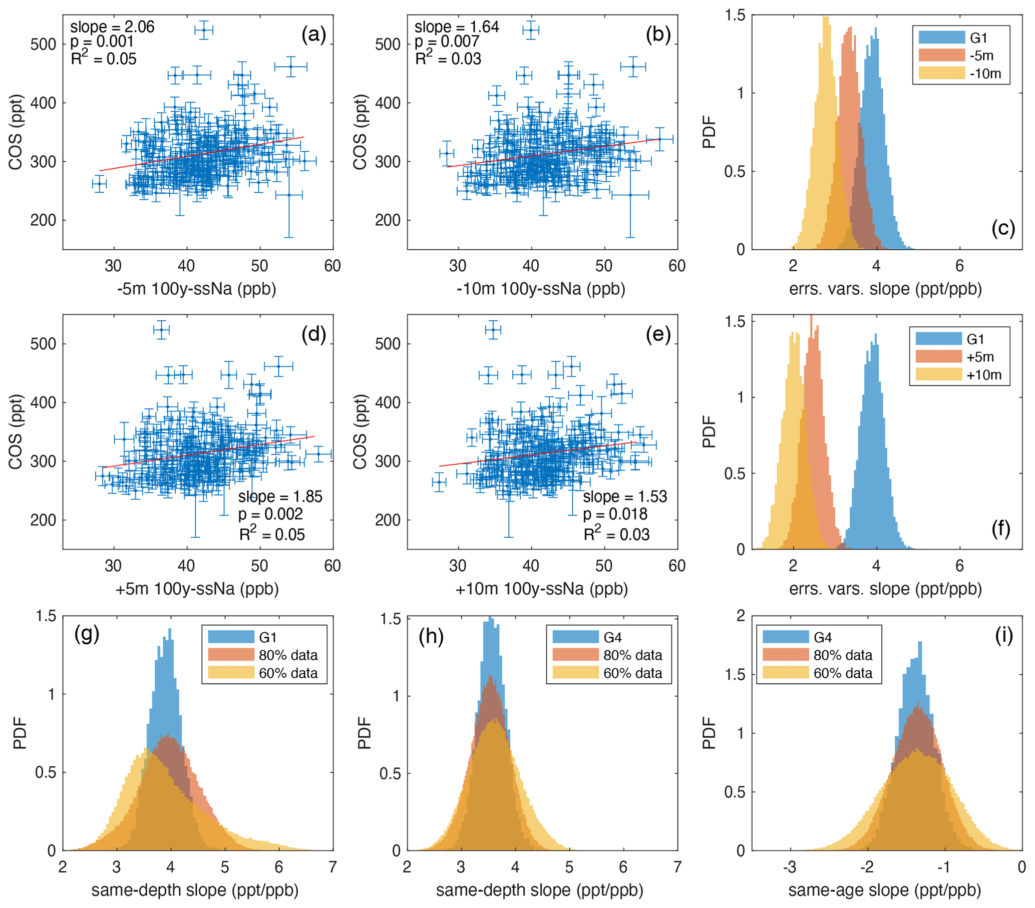
Figure A8Sensitivity tests for G1 and G4 analysis scenarios. (a) The 100-year ssNa vs. COS correlation with least-squares regression results. Here, ssNa is offset from COS measurement depths by −5 m. Panel (b) is the same as (a), but ssNa is offset from COS measurement depths by −10 m. (c) The errors-in-variables PDFs for (a) and (b) along with the G1 same-depth PDF from Fig. A5c. Panels (d–f) are the same as (a–c), but the offsets are +5 and +10 m. (g) Repeat of the G1 same-depth analysis by random sampling of the original data set at 80 % and 60 % in 20 simulations each. (h) Repeat of the G4 same-depth analysis by random sampling of the original data set at 80 % and 60 % in 20 simulations each. (i) Repeat of G4 same-age analysis by random sampling of the original data set at 80 % and 60 % in 20 simulations each.
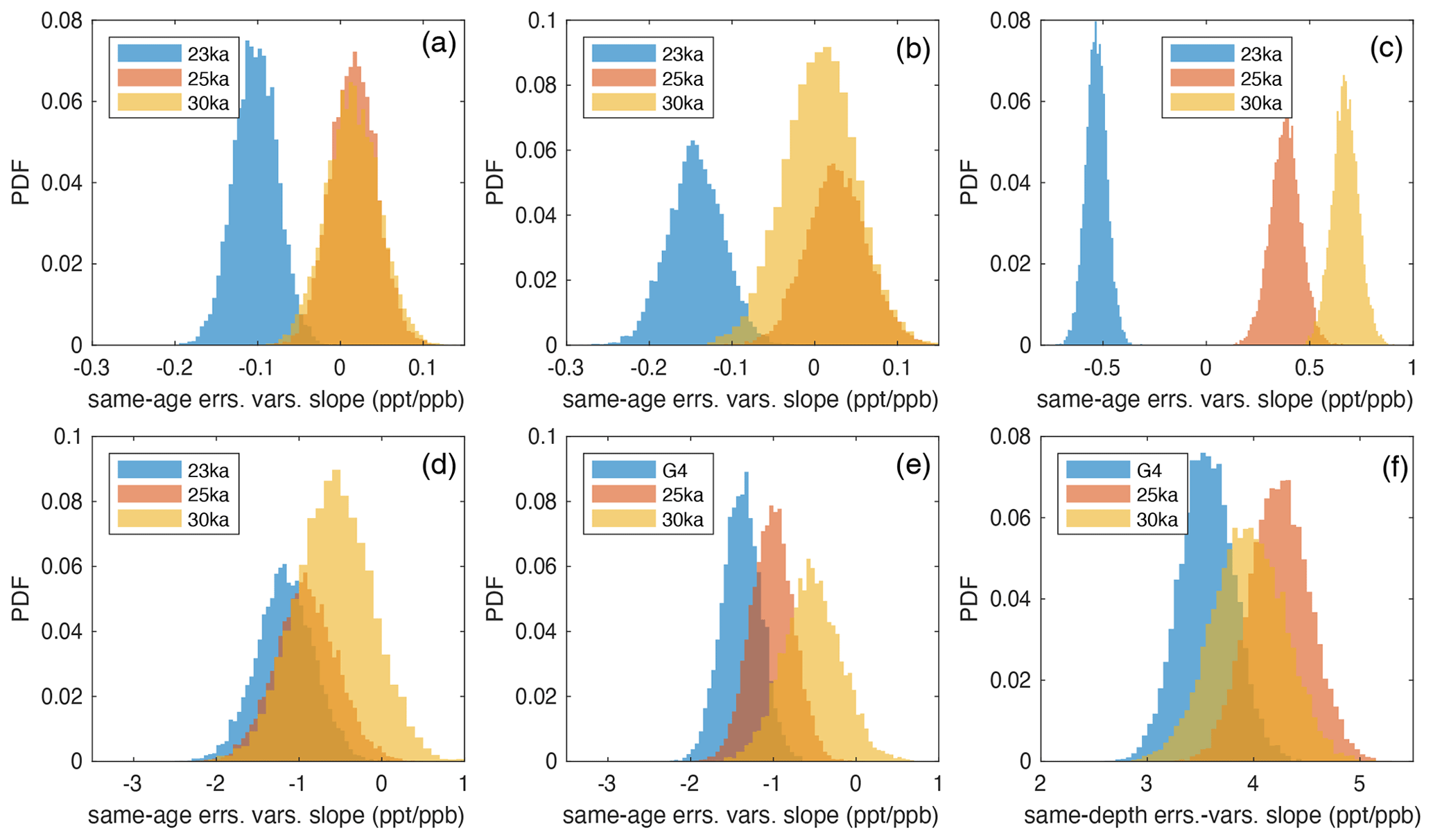
Figure A9(a) The errors-in-variables PDFs for the regression of the inverted 100-year ssNa interpolated to the SPC14 gas chronology at annual resolution vs. the 100-year ssNa record on ice chronology at annual resolution during three periods (>23, >25, and >30 ka). Panel (b) is the same as (a) except using 1100-year ssNa. Panel (c) is the same as (b) but at the ages of the COS measurements. (d) The errors-in-variables PDFs for the regression of the mean of the G4-corrected COS from Fig. 4b with the 1100-year ssNa. (e) The same-age results from a repeat of the G4 regression (Fig. 3c) for different temporal cutoffs. (f) The same-depth results from a repeat of the G4 regression (Fig. 3a) for different temporal cutoffs.
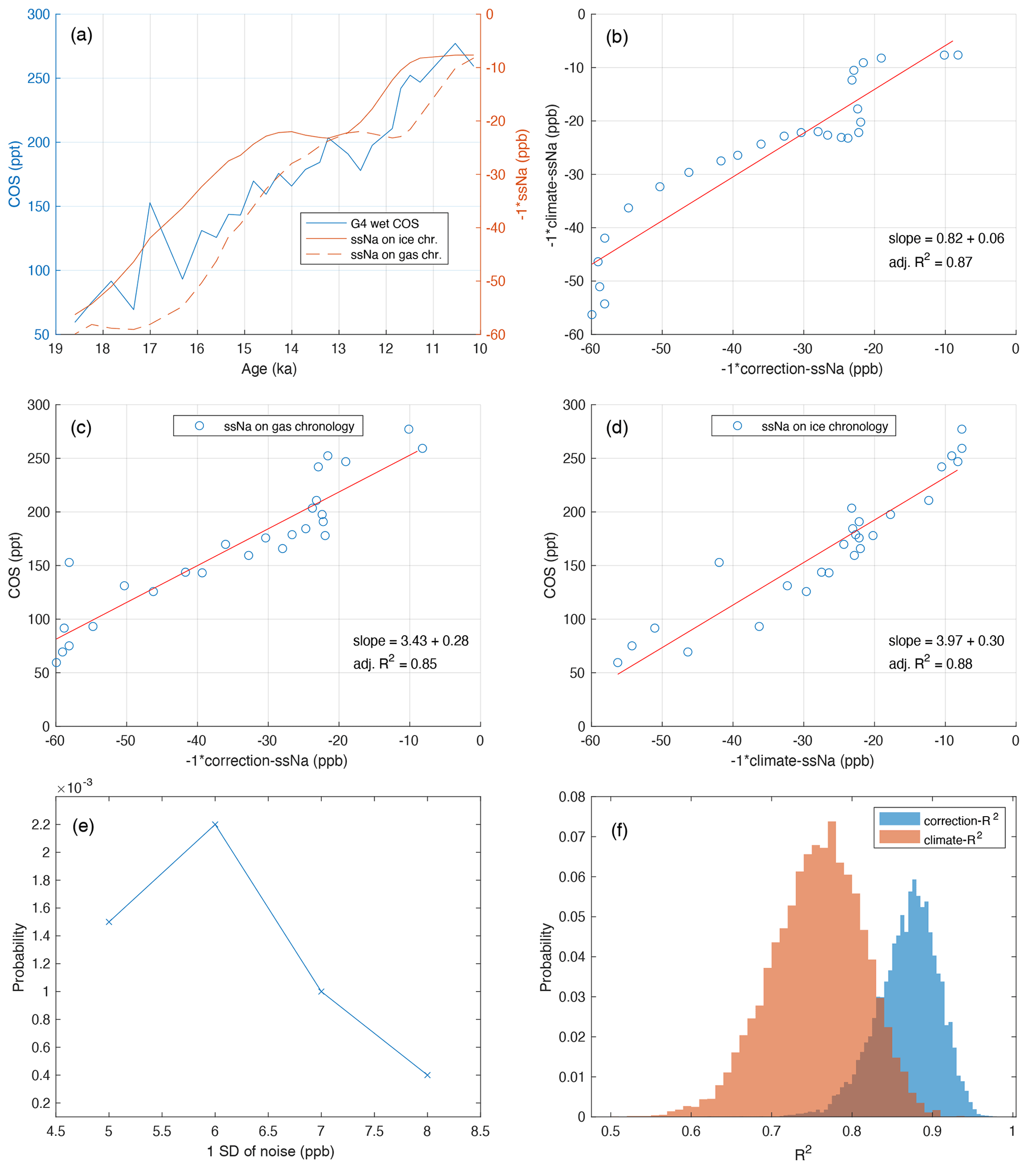
Figure A10(a) The corrected COS (G4) during the deglaciation (left y axis) and the correction ssNa and climate ssNa (right y axis). (b) The regression of the correction ssNa (x axis) vs. the climate ssNa (y axis). (c) The regression of the correction ssNa vs. COS. (d) The regression of the climate ssNa vs. COS. (e) The conditional probability of the climate R2 being higher than the correction R2, given the climate R2 is at least 0.88, at different levels of random noise. (f) The PDFs of the correction R2 and the climate R2 at 6 ppb noise.
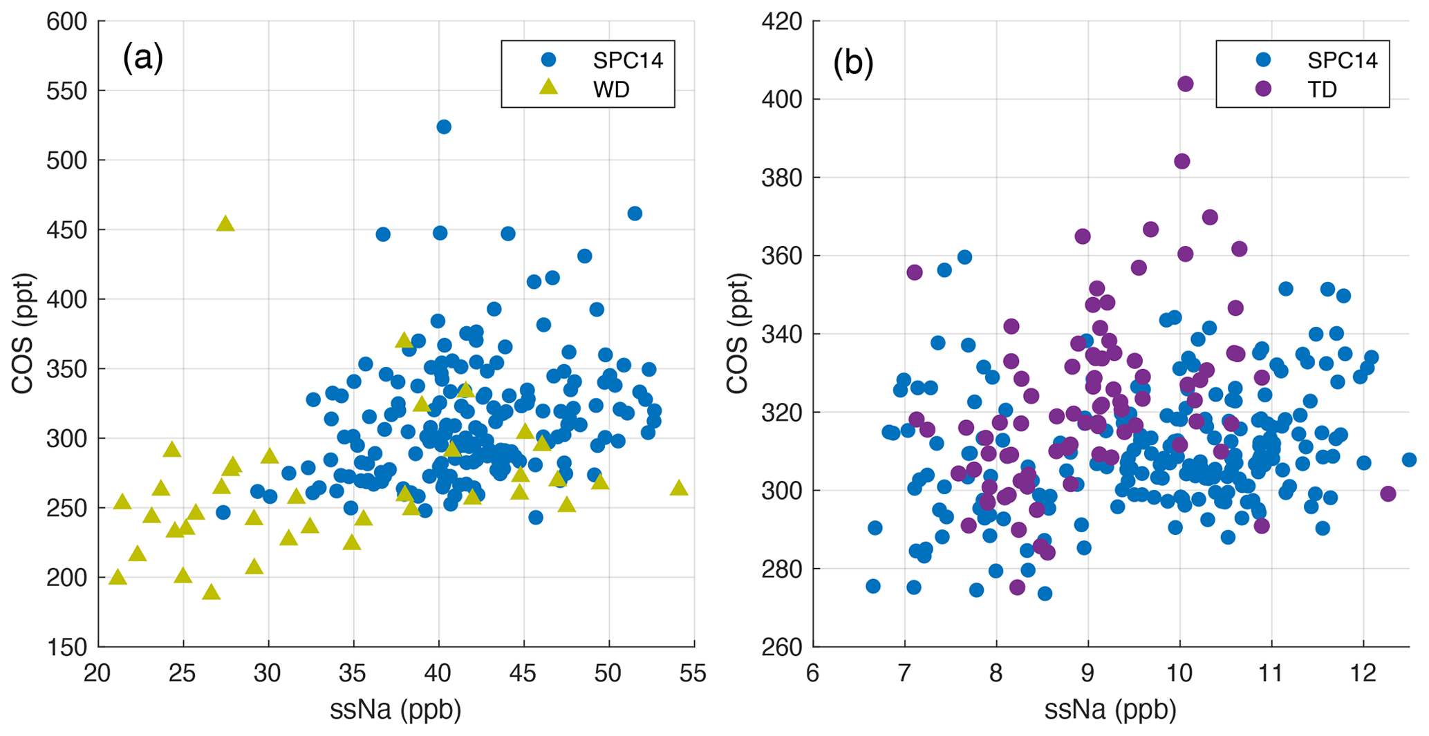
Figure A11The 100-year ssNa vs. measured COS levels. The ssNa for the WD and TD ice cores is calculated using Na+ and Ca2+ measurements from the respective cores (McConnell et al., 2017; Steig et al., 2000). (a) The data used in the G1 scenario (Fig. 2c) for SPC14 are compared with all data from WD older than 11 ka. (b) The data used in the H1 scenario (Fig. 2d) for SPC14 are compared with TD data younger than 8 ka.
We conducted two sensitivity tests for G1 and G4 scenarios. The first test is designed to test whether ssNa interpolated to the same depth as the COS samples is indeed the best predictor of the COS production. We repeat the G1 analysis with 100-year smooth ssNa interpolated to 5 and 10 m above and below the actual COS measurement depths (Fig. A8a–f). The significance of the ssNa–COS relationship deteriorates (PDFs move closer to zero) with offsets in either direction, confirming that ssNa interpolated to the same depths as the COS measurements is the best predictor of the COS production; however, this evidence alone is not sufficient to attribute the inferred production to a specific depth range in the firn.
In the second test, we explore the sensitivity of the regression results to random elimination of a subset of the measurements from the regressions. We repeat the G1 and G4 analyses with 20 subsets of the original COS data set (total of 40 simulations). Data in each subset are randomly picked without replacement to sample 80 % and 60 % of the full data set. In G1 (Fig. A8g), the mean slope value of the same-depth regression is not sensitive to the reduction in the amount of data included in the analysis, but the shape of the distribution and the significance are sensitive to this change. In G4 (Fig. A8h and i), the simultaneous same-depth and same-age regression results are robust with respect to the reduction in the data amount, with some reduction in significance at 20 % data reduction and more at 40 %, but they have minimal impact on the mean value and the shape of the distribution. These results demonstrate that G4 results are more robust with respect to data density than those of G1.
The same-age correlation analyses display an anti-correlation between ssNa and COS during the glacial period (52–23 ka) even when such analyses are conducted independently between measured COS and ssNa without a simultaneous same-depth correction. Simultaneous same-depth regression strengthens this relationship (Fig. 3c). Here, we explore whether this strengthening could be resulting from the fact that the applied same-depth correction itself is anti-correlated with the ssNa record. These tests are akin to testing the autocorrelation of the ssNa record at a given lag, but the delta age for the ice core is used instead of a fixed lag.
We set up three control scenarios. In the first scenario, we interpolate an inverted (multiplied by −1 to simulate the ssNa correction to the COS record) 100-year smooth ssNa record to the SPC14 gas chronology at annual resolution and then regress it against the original 100-year ssNa record on ice chronology for the same depths over periods older than 23, 25, and 30 ka (Fig. A9a). The second scenario is identical to the first, except we used the 1100-year smooth ssNa record (Fig. A9b). The third scenario is a repeat of the second at lower and irregular resolution, using only the 1100-year ssNa data interpolated to the COS measurement depths (Fig. A9c). All three control scenarios reveal significant but small negative slopes for the 23 ka cutoff, but truncating the analyses with the 25 or 30 ka cutoffs results in either no significant correlation or a positive correlation.
The three control scenarios can be compared with the same-age regressions between ssNa and COS corrected for excess COS using the same-depth relationship under G4. When the corrected COS from G4 is regressed with the same-age 1100-year ssNa, we find that it is more robust against the temporal cutoffs (Fig. A9d). This is slightly different from what is done in G4 because we do not conduct a simultaneous same-depth regression. Repeats of the G4 regression itself using different temporal cutoffs reaffirm that the same-age anticorrelation between ssNa and COS during 52–23 ka results primarily from variance in the measured COS mixing ratios and not from the applied same-depth correction (Fig. A9e). Further, the same-depth regression results do not vary significantly or show any sign of deterioration at different temporal cutoffs (Fig. A9f).
Here, we investigate whether there is any explicit statistical evidence that the increase in the inferred atmospheric COS record concurrent with the deglaciation during 19–10 ka is climate driven. The same-depth ssNa correction alone would result in a temporal COS trend that looks like the inverted ssNa record on the gas age scale (correction ssNa), whereas the true climate signal in the ssNa record is evident on the ice chronology (climate ssNa). The corrected COS record from G4 is regressed against the 1100-year smooth (G4) correction ssNa and against the climate ssNa (Fig. A10). The R2 statistic for the regression vs. the correction ssNa is 0.85 (Fig. A10c), indicating the magnitude of the deglacial COS rise is set primarily by the ssNa correction. The R2 of the regression vs. the climate ssNa should be comparatively low if the COS measurements merely introduce random noise into the corrected COS record, but the climate R2 is 0.88 and higher than the correction R2 (Fig. A10c vs. d).
It is possible to estimate the probability that we would observe these climate R2 and correction R2 values coincidentally. To do so, we introduce random noise to the correction ssNa, and we then regress against the actual correction ssNa (itself without the noise) and separately against the climate ssNa (also without noise) in 10 000 simulations, calculating the correction R2 and climate R2 for each instance. We find that the conditional probability of climate R2 being higher than the correction R2, given that climate R2 is equal to or higher than 0.88, peaks at about p=0.002 with 6 ppb (±1 SD) of added noise (Fig. A11e). The probabilities are lower at lower noise because the correction R2 approaches 1 and also lower at higher noise because the climate R2 decreases rapidly. It is highly probable that the wet COS measurements from the deglaciation include a climate signal, which is retained during the same-depth ssNa correction, resulting in an inferred atmospheric COS record that is more similar to the deglacial climate signal than the inverse of the applied ssNa correction.
The solubility of gases in the ocean is temperature dependent. Sea surface temperature rises during the deglaciation and this effect alone should result in an increase in gas flux out of the ocean due to decreased solubility. A +1 °C change in temperature results in a less than 5 % decrease in the solubilities of COS, CS2, and DMS over a range of 0 to 30 °C (DeBruyn et al., 1995; Elliot et al., 1989). Present-day ocean CS2 flux correlates with temperature and can increase by about 10 % °C−1 (Xie and Moore, 1999); this effect is too high to be solely due to the temperature effect on CS2 solubility. Direct COS emissions are buffered against temperature increases because as solubility decreases, the hydrolysis loss rate increases at a faster rate, with +1 °C change in temperature resulting in about a 10 % rise in the COS hydrolysis rate constant. The hydrolysis of COS is also sensitive to pH and slows down by about 5 % per 0.1 unit decrease at pH 8 (Elliot et al., 1989). For the direct COS flux, the net impact of a +1 °C temperature increase coupled with a 0.1 unit decrease in pH is close to zero. It is not possible to drive large changes in ocean–atmosphere gas fluxes via temperature effects on gas solubility or via the coupled effects of temperature and pH on COS hydrolysis.
Brühl et al. (2012) calculated a radiative impact of −0.007 W m−2 for about a 30 % (roughly 150 ppt) increase in atmospheric COS during the 20th century due to anthropogenic emissions. They also estimate that the radiative impact of the same amount of COS as a greenhouse gas in the troposphere is 0.003 W m−2, yielding a net impact of −0.004 W m−2.
The radiative impact of increased atmospheric COS depends on the emission geometry. This has been estimated in chemistry-climate model experiments with two distinct emission geometries (Quaglia et al., 2022). In the first model experiment, COS was injected into the atmosphere using the geographic distribution of present-day anthropogenic emissions at the surface, thus the emissions occur primarily over land in the Northern Hemisphere where the terrestrial uptake is also strong. In the second model experiment, COS was injected at the tropical tropopause, which enables quick dispersion into the stratosphere. The location of the emissions impacts the relative increase in the tropospheric vs. stratospheric mixing ratios of COS. In the troposphere, COS acts primarily as a greenhouse gas and has a positive radiative impact. In the stratosphere, COS acts primarily as a source of sulfate aerosol with a negative radiative impact. The model also incorporates indirect radiative effects via ozone, methane, and stratospheric water vapor.
The net (tropospheric plus stratospheric) radiative impact of a 40 Tg S yr−1 emission increase in the first experiment is −1.3 W m−2. The net radiative impact of a 6 Tg S yr−1 emission increase in the second experiment is −1.5 W m−2. In the first and second modeling experiments, the tropospheric mixing ratio of COS stabilizes at 35 and 5 ppb, respectively. Assuming linear scaling, these sensitivities imply −0.006 W m−2 (first experiment) and −0.05 W m−2 (second experiment) net radiative impacts for a 150 ppt increase in tropospheric COS. The deglacial increase in COS emissions is largely oceanic in origin, and hence it is primarily in the boundary layer and in the Southern Hemisphere. The radiative impact estimates from the two model experiments should be considered unrealistic lower and upper bounds. The best estimate may be closer to the lower bound estimate from the first model experiment.
The underlying COS data set is available at https://www.usap-dc.org/view/dataset/601270 (Aydin, 2020). The underlying ssNa data set is available at https://www.usap-dc.org/view/dataset/601754 (Winski, 2023). The ssNa-corrected COS records are available in the Supplement as data files.
Sample Stan codes used in the statistical modeling are provided as a Supplement codes S1 and S2 in the Supplement document. The supplement related to this article is available online at: https://doi.org/10.5194/cp-20-1885-2024-supplement.
MA, MRN, ESS, CFL, TH, KJC, DW, DF, and EO developed the measurement methods and conducted the measurements. MA and GLB developed the data analysis methodology. MA wrote the original draft. MA, ESS, GLB, MW, DW, and MRN revised and edited the manuscript.
The contact author has declared that none of the authors has any competing interests.
Publisher's note: Copernicus Publications remains neutral with regard to jurisdictional claims made in the text, published maps, institutional affiliations, or any other geographical representation in this paper. While Copernicus Publications makes every effort to include appropriate place names, the final responsibility lies with the authors.
We thank U.S. Ice Drilling Program and the National Science Foundation Ice Core Facility for the drilling and curation of the ice cores.
This research has been supported by National Science Foundation (grant nos. 1443470 and 1917485) and the Simons Foundation (grant nos. 549931 and 645921).
This paper was edited by Kathleen A. Wendt and reviewed by Wu Sun and one anonymous referee.
Ahn, J. and Brook, E. J.: Atmospheric CO2 and climate from 65 to 30 ka B. P., Geophys. Res. Lett., 34, L10703, https://doi.org/10.1029/2007GL029551, 2007.
Anderson, R. F., Ali, S., Bradtmiller, L. I., Nielsne, H. H., and Burckle, L. H.: Wind-driven upwelling in the Southern Ocean and the deglacial rise in atmospheric CO2, Science, 323, 1443–1448, https://doi.org/10.1126/science.1167441, 2009.
Andreae, M. O.: Ocean-atmosphere interactions in the global biogeochemical sulfur cycle, Mar. Chem., 30, 1–29, 1990.
Aydin, M.: SPC14 carbonyl sulfide, methyl chloride, and methyl chloride measurements from South Pole, Antarctica, USAP-DC [data set], https://www.usap-dc.org/view/dataset/601270 (last access: 19 August 2024), 2020.
Aydin, M., Williams, M. B., and Saltzman, E. S.: Feasibility of reconstructing paleoatmospheric records of selected alkanes, methyl halides, and sulfur gases from Greenland ice cores, J. Geophys. Res., 112, D07312, https://doi.org/10.1029/2006JD008027, 2007.
Aydin, M., Fudge, T. J., Verhulst, K. R., Nicewonger, M. R., Waddington, E. D., and Saltzman, E. S.: Carbonyl sulfide hydrolysis in Antarctic ice cores and an atmospheric history for the last 8000 years, J. Geophys. Res.-Atmos., 119, 8500–8514, https://doi.org/10.1002/2014JD021618, 2014.
Aydin, M., Campbell, J. E., Fudge, T. J., Cuffey, K. M., Nicewonger, M. R., Verulst, K. R., and Saltzman, E. S.: Changes in atmospheric carbonyl sulfide over the last 54 000 years inferred from measurements in Antarctic ice cores, J. Geophys. Res.-Atmos., 121, 1943–1954, https://doi.org/10.1002/2015JD024235, 2016.
Aydin, M., Britten, G. L., Montzka, S. A., Buizert, C., Primeau, F., Petrenko, V., Battle, M. B., Nicewonger, M. R., Patterson, J., Hmiel, B., and Saltzman, E. S.: Anthropogenic impacts on atmospheric carbonyl sulfide since the 19th century inferred from polar firn air and ice core measurements, J. Geophys. Res.-Atmos., 125, e2020JD033074, https://doi.org/10.1029/2020JD033074, 2020.
Bereiter, B., Eggleston, S., Schmitt, J., Nehrbass-Ahles, C., Stocker, T. F., Fischer, H., Kipfstuhl, S., and Chappella, J.: Revision of the EPICA Dome C CO2 record from 800 to 600 ka before present, Geophys. Res. Lett., 42, 542–549, https://doi.org/10.1002/2014GL061957, 2015.
Berry, J., Wolf, A., Campbell, J. E., Baker, I., Blake, N., Blake, D., Denning, A. S., Kawa, S. R., Montzka, S. A., Seibt, U., Stimler, K., Yakir, D., and Zhu, Z.: A coupled model of the global cycles of carbonyl sulfide and CO2: A possible new window on the carbon cycle, J. Geophys. Res.-Biogeo., 118, 842–852, https://doi.org/10.1002/jgrg.20068, 2013.
Bock, M., Schmitt, J., Beck, J., and Fischer, H.: Glacial/interglacial wetland, biomass burning, and geologic methane emissions constrained by dual stable isotopic CH4 ice core records, P. Natl. Acad. Sci. USA, 114, E5778–E5786, https://doi.org/10.1073/pnas.1613883114, 2017.
Boucher, O., Randall, D., Artaxo, P., Bretherton, C., Feingold, G., Forster, P., Kerminen, V.-M., Kondo, Y., Liao, H., Lohmann, U., Rasch, P., Satheesh, S. K., Sherwood, S., Stevens, B., and Zhang, X. Y.: Clouds and Aerosols, in: Climate Change 2013: The Physical Science Basis. Contribution of Working Group I to the Fifth Assessment Report of the Intergovernmental Panel on Climate Change, edited by: Stocker, T. F., Qin, D., Plattner, G.-K., Tignor, M., Allen, S. K., Boschung, J., Nauels, A., Xia, Y., Bex, V., and Midgley, P. M., Cambridge University Press, Cambridge, United Kingdom and New York, NY, USA, https://www.ipcc.ch/site/assets/uploads/2018/02/WG1AR5_Chapter07_FINAL-1.pdf (last access: 26 August 2024), 2013.
Bowen, H. J. M.: Environmental chemistry of the elements, Academic Press, London UK, 333 pp., ISBN 978-0-12-120450-1, 1979.
Brühl, C., Lelieveld, J., Crutzen, P. J., and Tost, H.: The role of carbonyl sulphide as a source of stratospheric sulphate aerosol and its impact on climate, Atmos. Chem. Phys., 12, 1239–1253, https://doi.org/10.5194/acp-12-1239-2012, 2012.
Burke, A. and Robinson, L. F.: The Southern Ocean's role in carbon exchange during the last deglaciation, Science, 335, 557–561, https://doi.org/10.1126/science.1208163, 2012.
Butler, J. H., Battle, M. B., Bender, M. L., Montzka, S. A., Clarke, A. D., Saltzman, E. S., Sucher, C. M., Severignhaus, J. P., and Elkins, J. W.: A record of atmospheric halocarbons during the twentieth century from polar firn air, Nature, 399, 749–755, https://doi.org/10.1038/21586, 1999.
Carpenter, B., Gelman, A., Hoffman, M. D., Lee, D., Goodrich, B., Betancourt, M., Brubaker, M. A., Guo, J., Li, P., and Riddell, A.: Stan: A Probabilistic Programming Language, J. Stat. Softw., 76, 1–32, https://doi.org/10.18637/jss.v076.i01, 2017.
Charlson, R. J., Lovelock, J. E., Andreae, M. O., and Warren, S. G.: Oceanic phytoplankton, atmospheric sulphur, cloud albedo and climate, Nature, 326, 655–661, https://doi.org/10.1038/326655a0, 1987.
Ciais, P., Tagliabue, A., Cuntz, M., Bopp, L., Scholze, M., Hoffman, G., Lourantou, A., Harrison, S. P., Prentice, I. C., Kelley, D. I., Koven, C., and Piao, S. L.: Large inert carbon pool in the terrestrial biosphere during the last glacial maximum, Nat. Geosci., 5, 74–79, https://doi.org/10.1038/ngeo1324, 2012.
Costa, K. M., Jacobel, A. W., McManus, J. F., Anderson, R. F., Winckler, G., and Thiagarajan, N.: Productivity patterns in the equatorial Pacific over the last 30 000 years, Global Biogeochem. Cy., 31, 850–865, https://doi.org/10.1002/2016GB005579, 2017.
Curran, M. A. J. and Jones, G. B.: Dimethyl sulfide in the Southern Ocean: Seasonality and flux, J. Geophys. Res., 105, 20451–20459, https://doi.org/10.1029/2000JD900176, 2000.
Cutter, G. A., Cutter, L. S., and Filippino, K. C.: Sources and cycling of carbonyl sulfide in the Sargasso Sea, Limnol. Oceanogr., 49, 555–565, https://doi.org/10.4319/lo.2004.49.2.0555, 2004.
De Bruyn, W. L., Swartz, E., Hu, J. H., Shorter, J. A., Davidovits, P., Worsnop, D. R., Zahniser, M. S., and Kolb, C. E.: Henry's law solubilities and Setchenow coefficients for biogenic reduced sulfur species obtained from gas-liquid uptake measurements, J. Geophys. Res., 100, 7245–7251, https://doi.org/10.1029/95JD00217, 1995.
Elliot, S., Lu, E., and Rowland, F. S.: Rates and mechanisms for the hydrolysis of carbonyl sulfide in natural waters, Environ. Sci. Technol., 23, 458–461, 1989.
Epifanio, J. A., Brook, E. J., Buizert, C., Edwards, J. S., Sowers, T. A., Kahle, E. C., Severinghaus, J. P., Steig, E. J., Winski, D. A., Osterberg, E. C., Fudge, T. J., Aydin, M., Hood, E., Kalk, M., Kreutz, K. J., Ferris, D. G., and Kennedy, J. A.: The SP19 chronology for the South Pole Ice Core – Part 2: gas chronology, Δage, and smoothing of atmospheric records, Clim. Past, 16, 2431–2444, https://doi.org/10.5194/cp-16-2431-2020, 2020.
Faïn, X., Chappellaz, J., Rhodes, R. H., Stowasser, C., Blunier, T., McConnell, J. R., Brook, E. J., Preunkert, S., Legrand, M., Debois, T., and Romanini, D.: High resolution measurements of carbon monoxide along a late Holocene Greenland ice core: evidence for in situ production, Clim. Past, 10, 987–1000, https://doi.org/10.5194/cp-10-987-2014, 2014.
Fischer, H., Fundel, F., Ruth, U., Twarloh, B., Wegner, A., Udisti, R., Becagli, S., Castellano, E., Morganti, A., Severi, M., Wolff, E., Littot, G., Röthlisberger, R., Mulvaney, R., Hutterli, M. A., Kaufmann, P., Federer, U., Lambert, F., Bigler, M., Hansson, M., Jonsell, U., de Angelis, M., Boutron, C., Siggaard-Andersen, M.-L., Steffensen, J. P., Barbante, C., Gaspari, V., Gabrielli, P., and Wagenbach, D.: Reconstruction of millennial changes in dust emission, transport and regional sea ice coverage using the deep EPICA ice cores from the Atlantic and Indian Ocean sector of Antarctica, Earth Planet. Sc. Lett., 260, 340–354, https://doi.org/10.1016/j.epsl.2007.06.014, 2007.
Flöck, O. R., Andreae, M. O., and Dräger, M.: Environmentally relevant precursors of carbonyl sulfide in aquatic systems, Mar. Chem., 59, 71–85, https://doi.org/10.1016/S0304-4203(97)00012-1, 1997.
Freeman, E., Skinner, L. C., Waelbroeck, C., and Hodell, D.: Radiocarbon evidence for enhanced respired carbon storage in the Atlantic at the Last Glacial Maximum, Nat. Commun., 7, 11998, https://doi.org/10.1038/ncomms11998, 2016.
Glatthor, N., Hopfner, M., Baker, I. T., Berry, J., Campbell, J. E., Kawa, S. R., Krysztofiak, G., Leyser, A., Sinnhuber, B.-M., Stiller, G. P., Stinecipher, J., and von Clarmann, T.: Tropical sources and sinks of carbonyl sulfide observed from space, Geophys. Res. Lett., 42, 10082–10090, https://doi.org/10.1002/2015GL066293, 2015.
Goto-Azuma, K., Hirabayashi, M., Motoyama, H., Miyake, T., Kuramoto, T., Uemura, R., Igarashi, M., Iizuka, Y., Sakurai, T., Horikawa, S., Suzuki, K., Suzuki, T., Fujita, K., Kondo, Y., Hattori, S., and Fujii, Y.: Reduced marine phytoplankton sulphur emissions in the Southern Ocean during the past seven glacials, Nat. Commun., 10, 3247, https://doi.org/10.1038/s41467-019-11128-6, 2019.
Grannas, A. M., Jones, A. E., Dibb, J., Ammann, M., Anastasio, C., Beine, H. J., Bergin, M., Bottenheim, J., Boxe, C. S., Carver, G., Chen, G., Crawford, J. H., Dominé, F., Frey, M. M., Guzmán, M. I., Heard, D. E., Helmig, D., Hoffmann, M. R., Honrath, R. E., Huey, L. G., Hutterli, M., Jacobi, H. W., Klán, P., Lefer, B., McConnell, J., Plane, J., Sander, R., Savarino, J., Shepson, P. B., Simpson, W. R., Sodeau, J. R., von Glasow, R., Weller, R., Wolff, E. W., and Zhu, T.: An overview of snow photochemistry: evidence, mechanisms and impacts, Atmos. Chem. Phys., 7, 4329–4373, https://doi.org/10.5194/acp-7-4329-2007, 2007.
Ikeda, T., Fukazawa, H., Mae, S., Pepin, L., Duval, P., Champagnon, B., Lipenkov, V. Y., and Hondoh, T.: Extreme fractionation of gases caused by formation of clathrate hydrates in Vostok Antarctic ice, Geophys. Res. Lett., 26, 91–94, https://doi.org/10.1029/1998GL900220, 1999.
Ikeda-Fukazawa, T., Hondoh, T., Fukumura, T., Fukazawa, H., and Mae, S.: Variation in ratio of occluded air in Dome Fuji Antarctic ice, J. Geophys. Res., 106, 17799–17810, https://doi.org/10.1029/2000JD000104, 2001.
Jaccard, S. L., Hayes, C. T., Martinez-Garcia, A., Hodell, D. A, Anderson, R. F., Sigman, D. M., and Haug, G. H.: Two modes of change in Southern Ocean Productivity over the past million years, Science, 339, 1419–1423, https://doi.org/10.1126/science.1227545, 2013.
Jennerjahn, T. C.: Biogeochemical response of tropical coastal systems to present and past environmental change, Earth-Sci. Rev., 114, 19–41, https://doi.org/10.1016/j.earscirev.2012.04.005, 2012.
Jernigan, C. M., Fite, C. H., Vereecken, L., Berkelhammer, M. B., Rollins, A. W., Rickly, P. S., Novelli, A., Taraborrelli, D., Holmes, C. D., and Bertram, T. H.: Efficient production of carbonyl sulfide in the low-NOx oxidation of dimethyl sulfide, Geophys. Res. Lett., 49, e2021GL096838, https://doi.org/10.1029/2021GL096838, 2022.
Kettle, A. J., Kuhn, U., von Hobe, M., Kesselmeier, J., and Andreae, M. O.: Global budget of atmospheric carbonyl sulfide: Temporal and spatial variations of the dominant sources and sinks, J. Geophys. Res., 107, 4658, https://doi.org/10.1029/2002JD002187, 2002.
Khan, M. A. H., Bannan, T. J., Holland, R., Shallcross, D. E., Archibald, A. T., Matthews, E., Back, A., Allan, J., Coe, H., Artaxo, P., and Parcival, C. J.: Impacts of hydroperoxymethyl thioformate on the global marine sulfur budget, ACS Earth Space Chem., 5, 2577–2586, https://doi.org/10.1021/acsearthspacechem.1c00218, 2021.
King, A. C. F., Thomas, E. R., Pedro, J. B., Markle, B., Potocki, M., Jackson, S. L., Wolff, E., and Kalberer, M.: Organic compounds in a sub-Antarctic ice core: A potential suite of sea ice markers, Geophys. Res. Lett., 46, 9930–9939, https://doi.org/10.1029/2019GL084249, 2019.
King, M. D. and Simpson, W. R.: Extinction of UV radiation in Arctic snow at Alert, Canada (82° N), J. Geophys. Res., 106, 12499–12507, https://doi.org/10.1029/2001JD900006, 2001.
Köhler, P., Nehrbass-Ahles, C., Schmitt, J., Stocker, T. F., and Fischer, H.: A 156 ka smoothed history of the atmospheric greenhouse gases CO2, CH4, and N2O and their radiative forcing, Earth Syst. Sci. Data, 9, 363–387, https://doi.org/10.5194/essd-9-363-2017, 2017.
Kremser, S., Thomason, L. W., von Hobe, M., Hermann, M., Deshler, T., Timmreck, C., Toohey, M., Stenke, A., Schwarz, J. P., Weigel, R., Fueglistaler, S., Prata, F. J., Vernier, J.-P., Schlager, H., Barnes, J. E., Antuña-Marrero, J.-C., Fairlie, D., Palm, M., Mahieu, E., Notholt, J., Rex, M., Bingen, C., Vanhellemont, F., Bourassa, A., Plane, J. M. C., Klocke, D., Carn, S. A., Clarisse, L., Trickl, T., Neely, R., James, A. D., Rieger, L., Wilson, J. C., and Meland, B.: Stratospheric aerosol – Observations, processes, and impact on climate, Rev. Geophys., 54, 278–335, https://doi.org/10.1002/2015RG000511, 2016.
Ksionzek, K. B., Lechtenfeld, O. J., McCallister, Scmitt-Kopplin, P., Geuer, J. K., Geibert, W., and Koch, B. P.: Dissolved organic sulfur in the ocean: Biogeochemistry of a petagram inventory, Science, 354, 456–459, https://doi.org/10.1126/science.aaf7796, 2016.
Kuai, L., Worden, J. R., Campbell, J. E., Kulawik, S. S., Li, K.-F., Lee, M., Weidner, R. J., Montzka, S. A., Moore, F. L., Berry, J. A., Baker, I., Denning, A. S., Bian, H., Bowman, K. W., Liu, J., and Yung, Y. L.: Estimate of carbonyl sulfide tropical oceanic surface fluxes using aura tropospheric emission spectrometer observations, J. Geophys. Res.-Atmos., 120, 11012–11023, 2015.
Lana, A., Bell, T. G., Simo, R., Vallina, S. M., Ballabrera-Poy, J., Kettle, A. J., Dachs, J., Bopp, L., Saltzman, E. S., Stefels, J., Johnson, J. E., and Liss, P. S.: An updated climatology of surface dimethylsulfide concentrations and emission fluxes in the global ocean, Global Biogeochem. Cy., 25, GB1004, https://doi.org/10.1029/2010GB003850, 2011.
Laskin, A., Moffet, R. C., Gilles, M. K., Fast, J. D., Zaveri, R. A., Wang, B., Nigge, P., and Shutthanandan, J.: Tropospheric chemistry of internally mixed sea salt and organic particles: Surprising reactivity of NaCl with weak organic acids, J. Geophys. Res., 117, D15302, https://doi.org/10.1029/2012JD017743, 2012.
Legrand, M., Feniet-Saigne, C., Saltzman, E. S., Germain, C., Barkov, N. I., and Petrov, V. N.: Ice core record of oceanic emissions of dimethylsulfide during the last climate cycle, Nature, 350, 144–146, https://doi.org/10.1038/350144a0, 1991.
Lennartz, S. T., Marandino, C. A., von Hobe, M., Cortes, P., Quack, B., Simo, R., Booge, D., Pozzer, A., Steinhoff, T., Arevalo-Martinez, D. L., Kloss, C., Bracher, A., Röttgers, R., Atlas, E., and Krüger, K.: Direct oceanic emissions unlikely to account for the missing source of atmospheric carbonyl sulfide, Atmos. Chem. Phys., 17, 385–402, https://doi.org/10.5194/acp-17-385-2017, 2017.
Lennartz, S. T., von Hobe, M., Booge, D., Bittig, H. C., Fischer, T., Gonçalves-Araujo, R., Ksionzek, K. B., Koch, B. P., Bracher, A., Röttgers, R., Quack, B., and Marandino, C. A.: The influence of dissolved organic matter on the marine production of carbonyl sulfide (OCS) and carbon disulfide (CS2) in the Peruvian upwelling, Ocean Sci., 15, 1071–1090, https://doi.org/10.5194/os-15-1071-2019, 2019.
Lennartz, S. T., Marandino, C. A., von Hobe, M., Andreae, M. O., Aranami, K., Atlas, E., Berkelhammer, M., Bingemer, H., Booge, D., Cutter, G., Cortes, P., Kremser, S., Law, C. S., Marriner, A., Simó, R., Quack, B., Uher, G., Xie, H., and Xu, X.: Marine carbonyl sulfide (OCS) and carbon disulfide (CS2): a compilation of measurements in seawater and the marine boundary layer, Earth Syst. Sci. Data, 12, 591–609, https://doi.org/10.5194/essd-12-591-2020, 2020.
Lerman, A., Guidry M., Andersson, A. J., and Mackenzie, F. T.: Coastal ocean last glacial maximum to 2100 CO2-Carbonic Acid-Carbonate System: A Modeling Approach, Aquat. Geochem., 17, 749–773, https://doi.org/10.1007/s10498-011-9146-z, 2011.
Ma, J., Kooijmans, L. M. J., Cho, A., Montzka, S. A., Glatthor, N., Worden, J. R., Kuai, L., Atlas, E. L., and Krol, M. C.: Inverse modelling of carbonyl sulfide: implementation, evaluation and implications for the global budget, Atmos. Chem. Phys., 21, 3507–3529, https://doi.org/10.5194/acp-21-3507-2021, 2021.
Marcott, S. A., Bauska, T. K., Buizert, C., Steig, E. J., Rosen, J. L., Cuffey, K. M., Fudge, T. J., Severinghaus, J. P., Ahn, J., Kalk, M. L., McConnell, J. R., Sowers, T., Taylor, K. C., White, J. W. C., and Brook, E. J.: Centennial-scale changes in the global carbon cycle during the last deglaciation, Nature, 514, 616–619, https://doi.org/10.1038/nature13799, 2014.
McConnell, J. R., Burke, A., Dunbar, N. W., Köhler, P., Thomas, J. L., Arienzo, M. M., Chellman, N. J., Maselli, O. J., Sigl, M., Adkins, J. F., Baggenstos, D., Burkhart, J. F., Brook, E. J., Buizert, C., Cole-Dai, J., Fudge, T. J., Knorr, G., Graf, H.-F., Grieman, M. M., Iverson, N., McGwire, K. C., Mulvaney, R., Paris, G., Rhodes, R. H. Saltzmanm, E. S., Severinghaus, J. P., Steffensen, J. P., Taylor, K. C., and Winckler, G.: Synchronous volcanic eruptions and abrupt climate change ∼17.7 ka plausibly linked by stratospheric ozone depletion, P. Natl. Acad. Sci. USA, 114, 10035–10040, https://doi.org/10.1073/pnas.1705595114, 2017.
Modiri Gharehveran, M. and Shah, A. D.: Indirect photochemical formation of carbonyl sulfide and carbon disulfide in natural waters: Role of organic sulfur precursors, water quality constituents, and temperature, Environ. Sci. Technol., 52, 9108–9117, https://doi.org/10.1021/acs.est.8b01618, 2018.
Monnin, E., Steig, E. J., Siegenthaler, U., Kawamura, K., Schwander, J., Stauffer, B., Stocker, T. F., Morse, D. L., Barnola, J.-M., Bellier, B., Raynaud, D., and Fischer, H.: Evidence for substantial accumulation rate variability in Antarctica during the Holocene, through synchronization of CO2 in the Taylor Dome, Dome C and DML ice cores, Earth Planet. Sc. Lett., 224, 45–54, https://doi.org/10.1016/j.epsl.2004.05.007, 2004.
Montzka, S. A., Calvert, P., Hall, B. D., Elkins, J. W., Conway, T. J., Tans, P. P., and Sweeney, C.: On the global distribution, seasonality, and budget of atmospheric carbonyl sulfide and some similarities to CO2, J. Geophys. Res., 112, D09302, https://doi.org/10.1029/2006JD007665, 2007.
Mühl, M., Schmitt, J., Seth, B., Lee, J. E., Edwards, J. S., Brook, E. J., Blunier, T., and Fischer, H.: Methane, ethane, and propane production in Greenland ice core samples and a first isotopic characterization of excess methane, Clim. Past, 19, 999–1025, https://doi.org/10.5194/cp-19-999-2023, 2023.
Nelson, N. B. and Siegel, D. A.: The global distribution and dynamics of chromophoric dissolved organic matter, Annu. Rev. Mar. Sci., 5, 447–476, https://doi.org/10.1146/annurev-marine-120710-100751, 2013.
Nicewonger, M. R., Verhulst, K. R., Aydin, M., and Saltzman, E. S.: Preindustrial atmospheric ethane levels inferred from polar ice cores: A constraint on the geologic sources of atmospheric ethane and methane, Geophys. Res. Lett., 43, 214–221, https://doi.org/10.1002/2015GL066854, 2016.
Nicewonger, M. R., Aydin, M., Prather, M. J., and Saltzman, E. S.: Reconstruction of paleofire emissions over the past millennium from measurements of ice core acetylene, Geophys. Res. Lett., 47, e2019GL08510, https://doi.org/10.1029/2019GL085101, 2020.
Ohno, H., Lipenkov, V. Y., and Hondoh, T.: Air bubble to clathrate hydrate transformation in polar ice sheets: A reconsideration based on the new data from Dome Fuji ice core, Geophys. Res. Lett., 31, L21401, https://doi.org/10.1029/2004GL021151, 2004.
Peltier, W. R. and Fairbanks, R. G.: Global glacial ice volume and Last Glacial Maximum duration from an extended Barbados sea level record, Quaternary Sci. Rev., 25, 23–24, 3322–3337, https://doi.org/10.1016/j.quascirev.2006.04.010, 2006.
Pos, W. H., Riemer, D. D., and Zika, R. G.: Carbonyl sulfide and carbon monoxide in natural waters: evidence of a coupled production pathway, Mar. Chem., 62, 89–101, https://doi.org/10.1016/S0304-4203(98)00025-5, 1998.
Prentice, I. C., Harrison, S. P., and Bartlein, P. J.: Global vegetation and terrestrial carbon cycle changes after the last ice age, New Phytol., 189, 988–998, https://doi.org/10.1111/j.1469-8137.2010.03620.x, 2011.
Quaglia, I., Visioni, D., Pitari, G., and Kravitz, B.: An approach to sulfate geoengineering with surface emissions of carbonyl sulfide, Atmos. Chem. Phys., 22, 5757–5773, https://doi.org/10.5194/acp-22-5757-2022, 2022.
Salamatin, A. N., Hondoh, T., Uchida, T., and Lipenkov, V. Y.: Post-nucleation conversion of an air bubble to clathrate air-hydrate crystal in ice, J. Cryst. Growth, 193, 197–218, https://doi.org/10.1016/S0022-0248(98)00488-6, 1998.
Sheng, J.-X., Weisenstein, D. K., Luo, B.-P., Rozanov, E., Stenke, A., Anet, J., Bingemer, H., and Peter, T.: Global atmospheric sulfur budget under volcanically quiescent conditions: Aerosol-chemistry-climate model predictions and validation, J. Geophys. Res.-Atmos., 120, 256–276, https://doi.org/10.1002/2014JD021985, 2015.
Solomon, S.: Stratospheric ozone depletion: A review of concepts and history, Rev. Geophys., 37, 275–316, https://doi.org/10.1029/1999RG900008, 1999.
Souney, J., Twickler, M. S., Aydin, M., Steig, E. S., Fudge, T. J., Street, L. V., Nicewonger, M. R., Kahle, E. C., Johnson, J. A., Kuhl, T. W., Casey, K. A., Fegyveresi, J. M., Nunn, R. M., and Hargreaves, G. M.: Core handling, transportation and processing for the South Pole ice core (SPICEcore) project, Ann. Glaciol., 62, 118–130, https://doi.org/10.1017/aog.2020.80, 2020.
Steig, E. J., Morse, D. L., Waddington, E. D., Stuiver, M., Grootes, P. M., Mayewski, P. A., Twickler, M. S., and Whitlow, S. I.: Wisconsinan and Holocene climate history from an ice core at Taylor Dome, Western Ross Embayment, Antarctica, Geogr. Ann. A, 82, 213–235, https://doi.org/10.1111/j.0435-3676.2000.00122.x, 2000.
Stimler, K., Montzka, S. A., Berry, J. A., Rudich, Y., and Yakir, D.: Relationship between carbonyl sulfide and CO2 during leaf gas exchange, New Phytol., 186, 869–878, https://doi.org/10.1111/j.1469-8137.2010.03218.x, 2010.
Stimler, K., Berry, J. A., Montzka, S. A., and Yakir, D.: Association between carbonyl sulfide uptake and 18Δ during gas exchange in C3 and C4 leaves, Plant Physiol., 157, 509–517, https://doi.org/10.1104/pp.111.176578, 2011.
Stoll, N., Bohleber, P., Dallmayr, R., Wilhelms, F., Barbante, C., and Weikusat, I.: The new frontier of microstructutal impurity research in polar ice, Ann. Glaciol., 64, 63–66, https://doi.org/10.1017/aog.2023.61, 2023.
Sun, W., Berry, J. A., Yakir, D., and Seibt, U.: Leaf relative uptake of carbonyl sulfide to CO2 seen through the lens of stomatal conductance-photosynthesis coupling, New Phytol., 235, 1729–1742, https://doi.org/10.1111/nph.18178, 2022.
Thomas, M. A., Suntharalingam, P., Pozzoli, L., Rast, S., Devasthale, A., Kloster, S., Feichter, J., and Lenton, T. M.: Quantification of DMS aerosol-cloud-climate interactions using the ECHAM5-HAMMOZ model in a current climate scenario, Atmos. Chem. Phys., 10, 7425–7438, https://doi.org/10.5194/acp-10-7425-2010, 2010.
Vehtari, A., Gelman, A., Simpson, D., Carpenter, B., and Bürkner, P.-C.: Rank-Normalization, Folding, and Localization: An Improved R_hat for Assessing Convergence of MCMC (with Discussion), Bayesian Anal., 16, 667–718, https://doi.org/10.1214/20-BA1221, 2021.
Vogt, M. and Liss, P. S.: Dimethyl sulfide and climate, in: Surface Ocean-Lower Atmosphere Processes, Chap. 12, edited by: Le Quere, C. and Saltzman, E. S., Wiley, https://doi.org/10.1029/2008GM000790, 2009.
Von Hobe, M., Cutter, G. A., Kettle, A. J., and Andreae, M. O.: Dark production: A significant source of oceanic COS, J. Geophys. Res., 106, 31217, https://doi.org/10.1029/2000JC000567, 2001.
Wang, S., Maltrud, M., Elliot, S., Cameron-Smith, P., and Jonko, A.: Influence of dimethyl sulfide on the carbon cycle and biological production, Biogeochemistry, 138, 49–68, https://doi.org/10.1007/s10533-018-0430-5, 2018a.
Wang, S., Maltrud, M. E., Burrows, S. M., Elliot, S. M., and Cameron-Smith, P.: Impacts of shifts in phytoplankton community on Clouds and Climate via the sulfur cycle, Global Biogeochem. Cy., 32, 1005–1026, https://doi.org/10.1029/2017GB005862, 2018b.
Whelan, M. E., Lennartz, S. T., Gimeno, T. E., Wehr, R., Wohlfahrt, G., Wang, Y., Kooijmans, L. M. J., Hilton, T. W., Belviso, S., Peylin, P., Commane, R., Sun, W., Chen, H., Kuai, L., Mammarella, I., Maseyk, K., Berkelhammer, M., Li, K.-F., Yakir, D., Zumkehr, A., Katayama, Y., Ogée, J., Spielmann, F. M., Kitz, F., Rastogi, B., Kesselmeier, J., Marshall, J., Erkkilä, K.-M., Wingate, L., Meredith, L. K., He, W., Bunk, R., Launois, T., Vesala, T., Schmidt, J. A., Fichot, C. G., Seibt, U., Saleska, S., Saltzman, E. S., Montzka, S. A., Berry, J. A., and Campbell, J. E.: Reviews and syntheses: Carbonyl sulfide as a multi-scale tracer for carbon and water cycles, Biogeosciences, 15, 3625–3657, https://doi.org/10.5194/bg-15-3625-2018, 2018.
Winckler, G., Anderson, R. F., Jaccard, S. L., and Marcantonio, F.: Ocean dynamics, not dust, have controlled equatorial Pacific productivity over the past 500 000 years, P. Natl. Acad. Sci. USA, 113, 6119–6124, https://doi.org/10.1073/pnas.1600616113, 2016.
Winski, D. A.: South Pole ice core sea salt and major ions, USAP-DC [data set], https://www.usap-dc.org/view/dataset/601754 (last access: 19 August 2024), 2023.
Winski, D. A., Osterberg, E. C., Kreutz, K. J., Ferris, D. G., Cole-Dai, J., Thundercloud, Z., Huang, J., Alexander, B., Jaegle, L., Kennedy, J. A., Larrick, C., Kahle, E. C., Steig, E. J., and Jones, T. R.: Seasonally resolved Holocene sea-ice variability inferred from South Pole ice core chemistry, Geophys. Res. Lett., 48, e2020GL091602, https://doi.org/10.1029/2020GL091602, 2021.
Wolff, E. W., Fischer, H., Fundel, F., Ruth, U., Twarloh, B., Littot, G. C., Mulvaney, R., Röthlisberger, R., de Angelis, M., Boutron, C. F., Hansson, M., Jonsell, U., Hutterli, M. A., Lambert, F., Kaufmann, P., Stauffer, B., Stocker, T. F., Steffensen, J. P., Bigler, M., Siggaard-Andersen, M. L., Udisti, R., Becagli, S., Castellano, E., Severi, M., Wagenbach, D., Barbante, C., Gabrielli P., and Gaspari, V.: Southern Ocean sea-ice extent, productivity and iron flux over the past eight glacial cycles, Nature, 440, 491–496, https://doi.org/10.1038/nature04614, 2006.
Xie, H. and Moore, R. M.: Carbon disulfide in the North Atlantic and Pacific oceans, J. Geophys. Res., 104, 5393, https://doi.org/10.1029/1998JC900074, 1999.
Zepp, R. G. and Andreae, M. O.: Factors affecting the photochemical production of carbonyl sulfide in seawater, Geophys. Res. Lett., 21, 2813–2816, https://doi.org/10.1029/94GL03083, 1994.
- Abstract
- Introduction
- Methods
- Results
- Discussion
- Conclusions
- Appendix A: Additional figures
- Appendix B: Sensitivity tests for G1 and G4 scenarios
- Appendix C: The validity of the glacial period same-age anticorrelation between ssNa and COS as a climate signal
- Appendix D: The COS rise concurrent with the deglaciation
- Appendix E: Temperature and pH effects on gas solubility and COS hydrolysis
- Appendix F: Calculation of the COS radiative impact
- Data availability
- Author contributions
- Competing interests
- Disclaimer
- Acknowledgements
- Financial support
- Review statement
- References
- Supplement