Orbitally forced environmental changes during the accumulation of a Pliensbachian (Lower Jurassic) black shale in northern Iberia

Lower Pliensbachian hemipelagic successions from the northern Iberian palaeomargin are characterized by the occurrence of organic-rich calcareous rhythmites of decimetre-thick limestone and marl beds as well as thicker black shale intervals. Understanding the genetic mechanisms of the cyclic lithologies and processes involved along with the nature of the carbon cycle is of primary interest. This cyclostratigraphic study, carried out in one of the black shale intervals exposed in Santiurde de Reinosa (Basque–Cantabrian Basin), reveals that the calcareous rhythmites responded to periodic environmental variations in the Milankovitch-cycle band and were likely driven by eccentricity-modulated precession.

The main environmental processes that determined the formation of the rhythmite were deduced on the basis of the integrated sedimentological, mineralogical, and geochemical study of an eccentricity bundle. The formation of precession couplets was controlled by variations in carbonate production and dilution by terrigenous supplies, along with periodic changes in bottom-water oxygenation. Precessional configurations with marked annual seasonality increased terrigenous input (by rivers or wind) to marine areas and boosted organic productivity in surface water. The great accumulation of organic matter on the seabed eventually decreased bottom-water oxygenation, which might also be influenced by reduced ocean ventilation. Thus, deposition of organic-rich marls and shales occurred when annual seasonality was maximal. On the contrary, a reduction in terrestrial inputs at precessional configurations with minimal seasonality diminished shallow organic productivity, which, added to an intensification of vertical mixing, contributed to increasing the oxidation of organic matter. These conditions also favoured greater production and basinward export of carbonate mud in shallow marine areas, causing the formation of limy hemipelagic beds. Short eccentricity cycles modulated the amplitude of precession-driven variations in terrigenous input and oxygenation of bottom seawater. Thus, the amplitude of the contrast between successive precessional beds increased when the Earth's orbit was elliptical and diminished when it was circular. The data also suggest that short eccentricity cycles affected short-term sea level changes, probably through orbitally modulated aquifer eustasy.

1 Introduction

As a consequence of the gravitational interaction between astronomical bodies, the Earth's axial orientation and orbit vary cyclically at timescales that range from tens of thousands to a few million years (Berger and Loutre, 1994). These variations in orbital configuration regulate the latitudinal and temporal distribution of solar radiation (insolation), which determines the contrast between seasons. These periodic changes in the climatic system can affect the evolution of a wide range of sedimentary environments, from terrestrial to deep marine (Einsele and Ricken, 1991). As the open ocean is hardly affected by processes that may erode the seabed or interrupt the continuous settling of fine-grained particles, deep-marine pelagic and hemipelagic sediments accumulate at a generally constant, but slow, rate (a few centimetres per thousand years). Thus, pelagic and hemipelagic successions from both oceanic sediment cores and outcrops contain accurate records of orbitally modulated, quasi-periodic climate change episodes (Hinnov, 2013). These periodic changes in the climatic system are generally recorded as cyclic stratigraphic successions, the so-called rhythmites, in both pelagic and hemipelagic successions (Einsele and Ricken, 1991).

Significant progress in Early Jurassic cyclostratigraphy has been made in the last few decades thanks to the study of exceptional orbitally modulated sedimentary records obtained from deep-marine environments of the peri-Tethyan realm (e.g. Cardigan and Cleveland basins by Hüsing et al., 2014; Ruhl et al., 2016; Storm et al., 2020; Pieńkowski et al., 2021; Paris Basin by Charbonnier et al., 2023). Although these studies provided relevant astrochronological information, they did not focus on the climatic and environmental impact of the orbital cycles. Other studies deduced a control of long-term orbital cycles on the Jurassic carbon cycle (Martinez and Dera, 2015; Ikeda et al., 2016; Hollar et al., 2021; Zhang et al., 2023), but the climatic and environmental influence of short-term cycles has been less studied (Hinnov and Park, 1999; Ikeda et al., 2016; Hollar et al., 2023).

The aim of this study is to analyse the climatic and environmental impact of short-term orbital cycles on Lower Jurassic deep-marine deposits. To this end, a hemipelagic alternation of limy and marl–shale beds was analysed in the Santiurde de Reinosa section (hereafter referred to as the Santiurde section), Basque–Cantabrian Basin (BCB), Cantabria province, Spain. In order to determine if sedimentation was orbitally forced, a cyclostratigraphic analysis of the hemipelagic rhythmites was undertaken. Subsequently, an integrated multiproxy study was performed in a selected interval of the section in order to disentangle what environmental factors influenced the formation of the hemipelagic rhythmites.

2 Geological setting

In Early Jurassic times the BCB was located to the south of the Armorican massif and to the north of the Iberian massif, within the Laurasian epicontinental seaway that connected the Boreal Sea with the northwestern Tethyan Ocean (Fig. 1a; Aurell et al., 2002; Rosales et al., 2004). Previous palaeogeographic reconstructions located the northern Iberian margin at approximately 30° N palaeo-latitude (Quesada et al., 2005; Osete et al., 2011). Hence, the emerged Iberian source area was located in the semiarid belt but close to the boundary with the humid climatic zone (temperate climate characterized by mega-monsoons; Dera et al., 2009; Deconinck et al., 2020), which made it especially sensitive to astronomically driven climate change. Such periodic climate change episodes alternately increased and decreased the influence of one or the other climatic belts (Martinez and Dera, 2015).

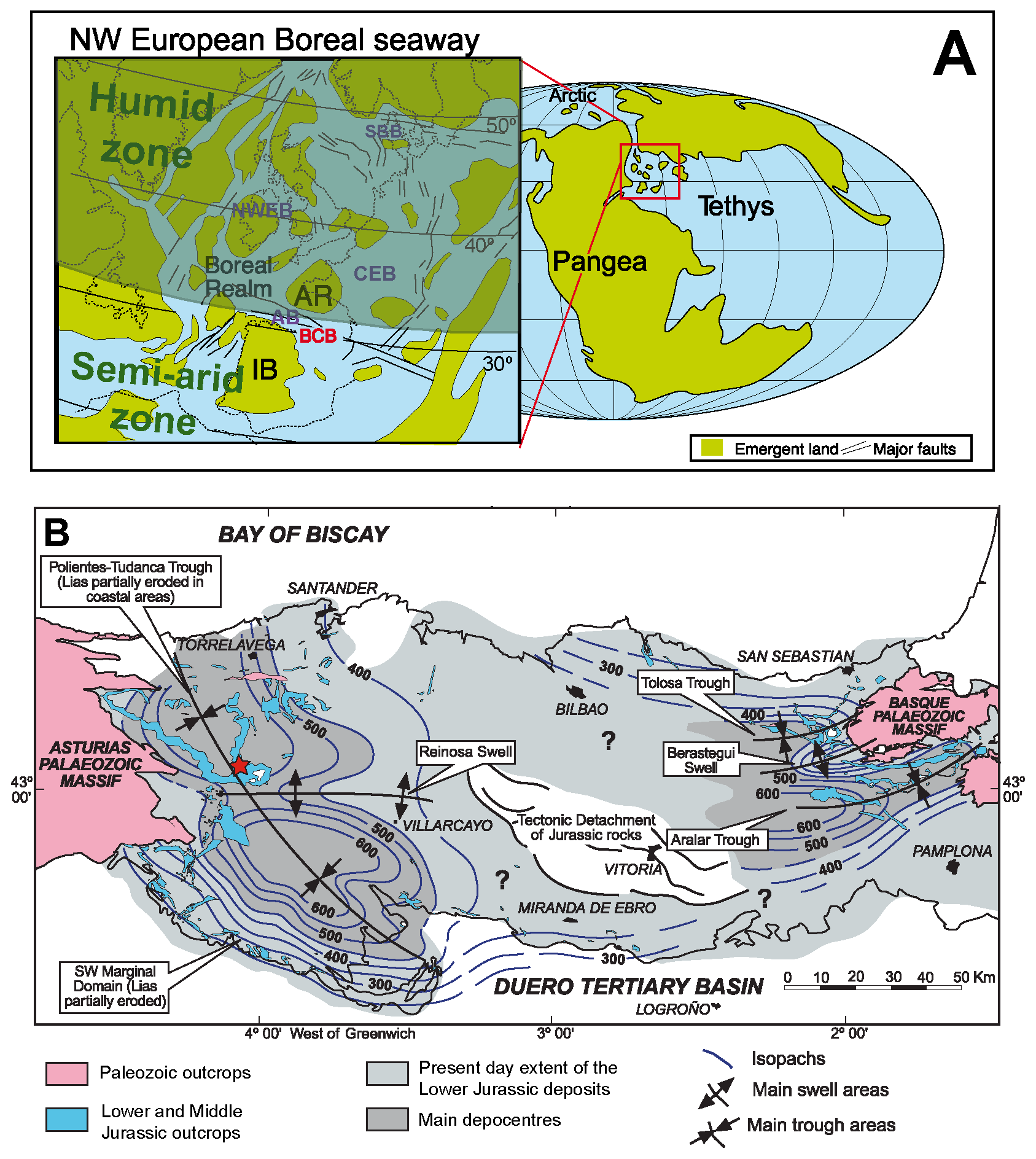
Figure 1 (a) Palaeogeography and climatic zonation (modified from Quesada et al., 2005; Dera et al., 2009; Osete et al., 2011) of western Europe in Early Jurassic times. IB: Iberian massif, AR: Armorican massif, AB: Asturian Basin, BCB: Basque–Cantabrian Basin, CEB: Central European Basin, NWEB: NW European Basin, SBB: southern boreal basin. (b) Simplified geographic and geological map of Lower and Middle Jurassic outcrops in the BCB area, with the location of the studied Santiurde section (red star). The superimposed isopach map shows the thickness of the Lower Jurassic rocks and the basin configuration in sedimentary troughs and swells (modified from Quesada et al., 2005).

Hettangian and lower Sinemurian deposits accumulated in evaporitic tidal flats and shallow carbonate ramps, whereas the overlying Sinemurian–Callovian succession accumulated in an open-marine, outer-ramp environment, which was generally in deep and quiet conditions below storm wave base (Aurell et al., 2002; Quesada et al., 2005). Hemipelagic sedimentation (sensu Henrich and Hüneke, 2011) prevailed in the outer ramp, as autochthonous pelagic production was mixed with periplatform carbonate advection and siliciclastic input from the southern continental margin. Differential subsidence during the Jurassic related to early mobilization of underlying Triassic salt resulted in the creation of several troughs in the BCB (Fig. 1b, Quesada et al., 2005).

Pliensbachian hemipelagic successions of the BCB (Camino Formation; Quesada et al., 2005) are characterized by the occurrence of three black shale intervals (BSIs), each several tens of metres thick (Braga et al., 1988; Quesada et al., 1997, 2005; Quesada and Robles, 2012; Rosales et al., 2001, 2004, 2006). These three BSIs are composed of alternating black shale layers and limestone–marly limestone beds and are separated from each other by decametric intervals devoid of black shale layers, in which only hemipelagic marls, marly limestones, and limestones occur. The three BSIs can be correlated with similar coeval deposits in neighbouring basins in Asturias (Borrego et al., 1996; Armendáriz et al., 2012; Bádenas et al., 2012, 2013; Gómez et al., 2016). Coeval organic-rich marine facies have also been observed in other Tethyan Lower Jurassic successions from Portugal (Silva et al., 2011), the United Kingdom (Hüsing et al., 2014), France (Bougeault et al., 2017), and Germany (Pieńkowski et al., 2008). The BCB Pliensbachian BSIs present relatively high organic carbon content (2 wt  %–6 wt  %), high pyrite concentrations, and scarce benthic faunas. Thermal maturity analysis showed that the BSIs found at the depocentres are overmature today, but they sourced the only oil reservoir discovered in inland Iberia (Quesada et al., 1997, 2005; Quesada and Robles, 2012; Permanyer et al., 2013). Pyrolysis of thermally immature samples from marginal areas showed total organic carbon values of up to 20 wt % and hydrogen index values up to 600–750 mg HC g⁻¹ of TOC 1987; Quesada et al., 1997). Analyses of organic matter (OM) showed that the assemblage is mainly composed of marine type-II kerogens, in which amorphous and algal material prevails (Quesada et al., 1997, 2005; Permanyer et al., 2013). More specifically, the analysis revealed a low content of gammaceranes, which suggests normal salinity conditions, and a great abundance of triclinic triterpanes, which can be associated with Tasmanites-type unicellular green algae with organic theca. In addition, the high content of isorenieratene byproducts, such as aryl-isoprenoids, indicates the occurrence of photosynthetic and sulfurous green algae communities (Chlorobiaceae) developed in oxygen-depleted conditions.

The Santiurde section studied herein is exposed at exit 144 of motorway A67 (UTM X411431.091 Y4769002.593; Fig. 1b), approximately 50 km southwest of Santander and 1 km northwest of a coeval section studied by others at the train station in the same locality (e.g. Rosales et al., 2001, 2004, 2006; Quesada et al., 2005; Fig. S1 in the Supplement). The studied succession begins with 2.5 m of alternating grey limestones and thin marlstones (Puerto Pozazal Formation), followed by 20 m of the lower part of the Pliensbachian Camino Formation, which are mainly made up of alternations of hemipelagic marls, limestones, and overmature black shales (Rosales et al., 2004; Quesada et al., 2005). Thus, the studied section includes the oldest BSI of the Camino Formation (BSI-1 in Fig. 2a), which according to regional biostratigraphy corresponds to the older part of the early Pliensbachian Uptonia jamesoni ammonite zone (Braga et al., 1988) and to the latter part of calcareous nannofossil zone NJ3 (Fraguas et al., 2015).

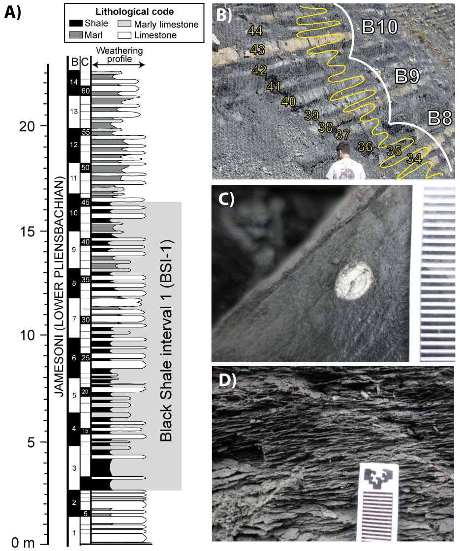
Figure 2 (a) Synthetic lithological log of the Santiurde section, including chronostratigraphy from Quesada et al. (2005) and Rosales et al. (2006). Columns B and C to the left of the lithological log correspond to bedding bundles and couplets, respectively, which were defined visually in the outcrop. (b) Calcareous couplets (yellow numbers) of bundles 8 to 10 (white numbers) in the Santiurde outcrop. The yellow curve shows the relief of successive beds in the outcrop (left, recessive; right, resistant), which is mainly determined by their carbonate content. The white curve shows bedding bundles. (c) Close-up of a marly limestone with a partly pyritized belemnite. (d) Close-up of a laminated black shale. Scale bar in millimetres.

3 Materials and methods

3.1 Cyclostratigraphic analysis of the Santiurde section

A detailed centimetre-scale stratigraphic log was measured in a 22.5 m thick succession that exposes the transition from the Puerto Pozazal Formation to the Pliensbachian Camino Formation. A broad range of sedimentological features, such as bed shape, thickness, composition, and palaeontological content and structures, were annotated. A total of 373 hand samples were collected, with a resolution of at least 3 samples per bed, avoiding visible skeletal components, burrows, and veins. The mass-normalized low-field magnetic susceptibility (MS) of the samples was measured using a Kappabridge KLY-3 instrument (Geophysika Brno) housed at the Geology department of the University of the Basque Country, Bilbao, Spain. Subsequently, rock-powder samples were obtained and stored in transparent antiglare prismatic vials, which were scanned in a dark room using a desktop office scanner. The average colour (RGB value) of the scanned images of rock-powder samples was determined using the ImageJ software and following the protocol in Dinarès-Turell et al. (2018) and Martinez-Braceras et al. (2023).

In order to carry out a cyclostratigraphic analysis, the Acycle software (Li et al., 2019) and the Astrochron package for R (Meyers et al., 2014) were used. The MS and colour data series were linearly interpolated and detrended first. Subsequently, power spectra were obtained using the 2π multitaper method (MTM) with three tapers, and confidence levels (CLs) were calculated following robust red-noise modelling (Mann and Lees, 1996). In addition, evolutive harmonic analysis (EHA; Meyers et al., 2001) and wavelet analyses (Torrence and Compo, 1998) were also carried out in order to examine the variability of the main frequency bands throughout the succession. Finally, the most significant frequency bands identified in the data series were isolated by Gaussian bandpass filtering.

3.2 Multiproxy analysis of bundle 9

An integrated analysis of several environmentally sensitive proxies was undertaken in the 19 beds found between 12.4 and 15.95 m of the stratigraphic succession. This interval includes a complete eccentricity bundle (B9, see results below), as well as the uppermost and lowermost couplets of the underlying and overlying bundles, respectively. A total of 57 samples, with a resolution of 3 samples per bed (21 shales, 9 marls, 12 marly limestones, and 15 limestones), were collected in order to perform a calcimetric analysis by measuring the carbonate percentage in 1 g of powder of each sample using a FOGL digital calcimeter (BD Inventions; accuracy of 0.5 %) housed at the University of the Basque Country. These samples were also analysed for inorganic δ¹³C_carb and δ¹⁸O_carb content at the Leibniz Laboratory for Radiometric Dating and Stable Isotope Research (Kiel University, Germany) using a Kiel IV carbonate preparation device connected to a Thermo Fisher Scientific MAT 253 mass spectrometer. Precision of all internal and external standards (NBS19 and IAEA-603) was better than ±0.05 ‰ for δ¹³C_carb and ±0.09 ‰ for δ18O_carb. All values are reported in the VPDB notation relative to NBS19.

In addition, one sample from the central part of each bed (19 samples) was studied for petrographic and scanning electron microscope (SEM) analysis, mineralogical content, elemental composition, and organic geochemistry. For the mineralogical and geochemical analyses, the samples were ground in the laboratory. Whole-rock mineralogy was obtained by analysing randomly oriented rock powder by X-ray diffraction (XRD) using a Philips PW1710 diffractometer (Malvern Panalytical, Malvern, UK) at the University of the Basque Country. The step size was 0.02° 2θ with a counting time of 0.5 s per step. Major and trace element concentrations were determined at the University of the Basque Country using a PerkinElmer Optima 8300 spectrometer (ICP-OES; PerkinElmer) and a Thermo XSeries 2 quadrupole inductively coupled plasma mass spectrometer (ICP-MS; Thermo Fisher Scientific) equipped with a collision cell, an interphase specific for elevated total dissolved solids (Xt cones), a shielded torch, and a gas dilution system. Analysis of the JG-2 granite standard and error estimates of each element showed that the uncertainty of the results corresponds to the 95 % confidence level. Finally, organic carbon (C_org) and organic nitrogen (N_org) contents, as well as their isotopic δ¹³C_org and δ¹⁵N_org values, were obtained by combustion of powdered and decarbonated samples in an elemental analyser Flash EA 1112 (Thermo Finnigan) connected to a DeltaV Advantage mass spectrometer (Thermo Fisher Scientific) at the University of A Coruña, Spain. Calibration of ¹³C_org and ¹⁵N_org was done against certificated standards USGS 40, USGS41a, NBS 22, and USGS24. Results are expressed in the VPDB notation, with accuracy (standard deviation) being ±0.15 ‰.

In order to explore compositional relationships and trends using comprehensive multi-elemental datasets, Pearson correlation coefficients (r) and their significance (p values) were estimated for pairs of variables using the SPSS 28 statistical package (IBM Corporation, SPSS statistics for Windows, version 28.0.1.1, 2022, Armonk, NY, USA). In addition, a multivariate factor analysis was undertaken with the aim of identifying the number of virtual variables (factors) that explains the highest percentage of the variability in the analysed dataset.

4 Results

4.1 General Santiurde section

4.1.1 Sedimentology and petrography

The outcrop displays a succession of decimetre-scale plane-parallel beds, in which light-coloured, bioturbated limestones or marly limestone beds resistant to weathering alternate with recessive, dark-coloured, laminated marls or shales (Fig. 2). In the outcrop, limestones and marly limestones were distinguished based on their hardness and colour, as prominent limestone beds are stiff and light grey, whereas marly limestones are less prominent, are softer, and show darker grey shades. The fossil record of both limestones and marly limestones is dominated by isolated ammonites, belemnites, and brachiopods (Fig. 2c), and burrows attributable to Chondrites and Planolites have been observed. Thin sections show mudstones and wackestones with dispersed benthic foraminifera, fragmented echinoderms, brachiopods, and pyritized bivalve shells (mainly pectinids) in a microspar matrix (Fig. 3a and c). Well-preserved placoliths of coccolithophorids and calcispheres were also identified by SEM (Fig. 3c and g). Some signs of diagenetic overprinting were identified, such as the occurrence of secondary cements, calcite overgrowths, early framboidal pyrite, and the growth of pyrite crystals in tests.

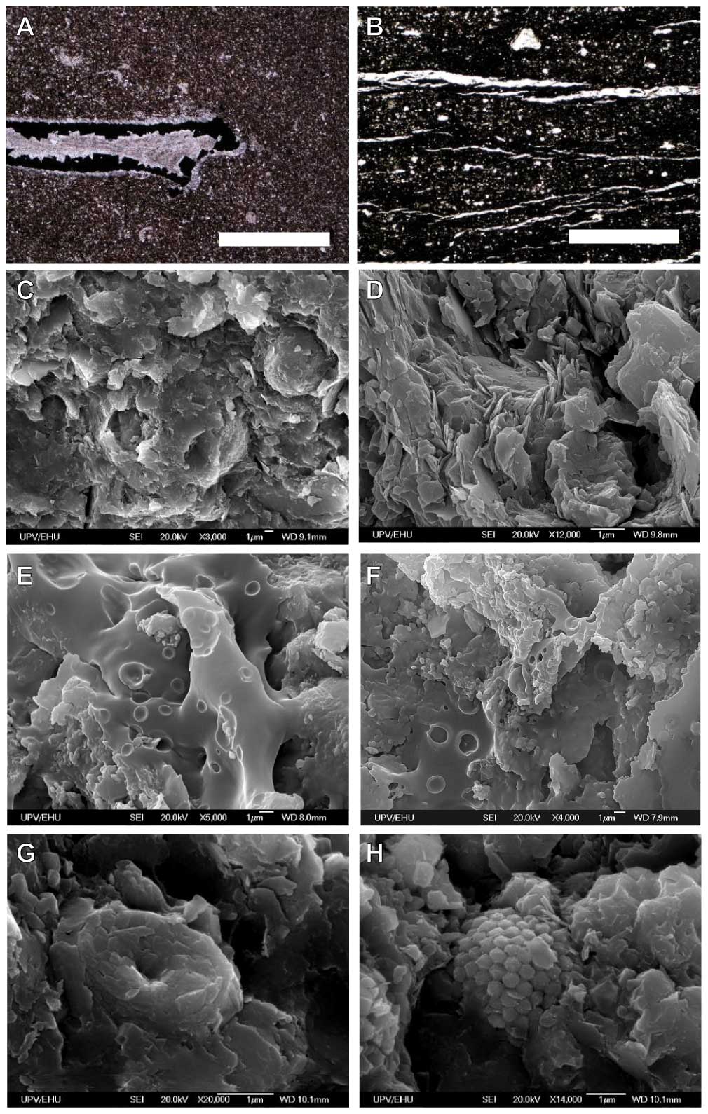
Figure 3 Petrographic views of limestone C41 (a) and shale C36 (b). The white bars represent 1 mm. (c) General texture of a limestone bed (couplet 37), showing partly dissolved and broken coccoliths and calcispheres. (d) General texture of a marly bed (couplet 37) with evidence of bioturbation. Panels (e) and (f) show probable biofilms. (f) Well-preserved coccolith. (g) Pyrite framboid.

Both marls and shales constitute friable beds more susceptible to weathering. Shales generally show darker colour and more prominent lamination (Fig. 2d), also observed in thin sections (Fig. 3b). The marls contain nekto-planktonic fossils (ammonites, belemnite, and calcareous unicellular algae) and evidence of benthonic communities (pyritized shells of bivalves and rhynchonellid brachiopods; trace fossils, such as Chondrites and Planolites), whereas the latter are absent in shales. This is confirmed by SEM analysis, as marls contain isolated, broken, and randomly oriented clay minerals that wrap well-preserved coccoliths and calcispheres with signs of bioturbation (Fig. 3c, d, and g). Nektonic organisms and planktonic unicellular algae also occur in shales, but benthonic fauna and bioturbation are virtually absent. SEM observations also showed that the lamination in shales is caused by the alternation of detrital components (mainly clays but also quartz) and organic components (such as bitumen, polymeric extracellular substances linked to biofilms, filamentous bacterial mats, or fungal hyphae; Fig. 3e and f). Pyrite framboids are more common in shales than in limy beds (Fig. 3h).

The abovementioned lithologies were used to define characteristic intervals in the succession (Fig. 2a). Based on the occurrence of black shale layers, the BSI-1 spans from 2.55 to 16.5 m (13.95 m thick). Black shale layers, with individual thicknesses of up to 79 cm, predominate in the lowermost part of the BSI, but intercalations of limestones, marly limestones, and marls become progressively more abundant upsection.

4.1.2 Bed arrangement

Cyclic bedding arrangements of different scales can be observed in the studied lithological alternation. The term couplet refers to the lithological pair of a weathered marl or shale bed and the overlying resistant limestone or marly limestone bed. A total of 62 calcareous bedding couplets (C1 to C62) were identified in the studied succession, with their individual thicknesses varying from 8 to 97 cm and averaging 36 cm (Figs. 2a and 4). These couplets extend beyond the studied section, as shown by a bed-by-bed correlation with the coeval railway section 1 km to the southeast (Fig. S1).

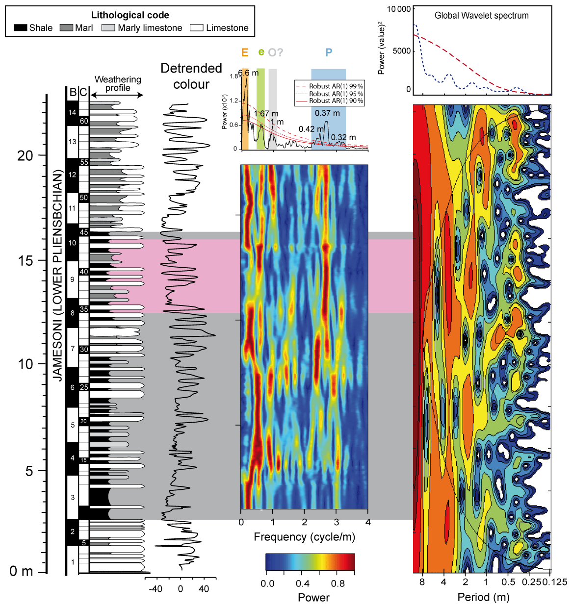
Figure 4 Stratigraphic log and chronostratigraphy (Quesada et al., 2005 and Rosales et al., 2006) of the studied section, showing the detrended colour curve. Bundles (B) and couplets (C) identified in the sedimentary alternation are numbered in ascending stratigraphic order. The grey background shows the extent of the Uptonia jamesoni BSI-1, and the pink interval in its upper part shows the interval studied herein in detail. The 2π MTM, EHA, and wavelet spectra of the colour data series show the occurrence of four main period bands: 30–42 cm cycles (in blue in the 2π MTM spectrum), interpreted as precession (P) couplets; 1 m cycles (grey), possibly related to obliquity (O?) cycles; 1.67 m cycles (green), representing short eccentricity (e) bundles; and 5–10 m cycles (peak at 6.6 m; orange), which correspond to long eccentricity (E) bundles.

The lithological contrast between the marl–shale and the (marly) limestone of the couplets is not constant throughout the succession, as some couplets are composed of shale and limestone beds but others are constituted of marl and marly limestone beds. These variations in the lithological contrast of couplets do not occur at random but allow the arrangement of the succession into bundles of five (four to six) couplets. Bundles, as defined herein, typically contain three prominent central couplets with great lithological contrast between successive limestone and marl–shale beds (e.g. couplets 34, 35, 38, 39, 40, and 43 in Fig. 2b), which are underlain and overlain by less obvious couplets with lower lithological contrast between successive marl and marly limestone beds (e.g. C36, C37, C41, C42 in Fig. 2b). In Santiurde, 12 complete bundles and another 2 incomplete bundles at the base and top of the section were defined, which range in thickness from 126 to 208 cm (average: 167.3 cm).

Two successive bundles can be readily observed in some intervals of the studied succession (e.g. B9 and B10 in Fig. 2b). However, the delimitation of bundles is not straightforward in other equally thick intervals (Fig. S1). These intervals with well-defined and less obvious bundles alternate regularly throughout the Santiurde section, which suggests the occurrence of a larger-scale (6.6 m thick) cyclic arrangement in the lithological succession.

4.1.3 Colour and magnetic susceptibility

Colour values (mean RGB) range from 69.87 to 158.99, averaging 102.73 (Fig. S1; Table S2). The colour curve oscillates in line with the lithological alternation, with colour values generally being higher in limestones and marly limestones (average of 115.14) than in intervening marls or shales (average of 90.71). The variations in colour values are greater in the central couplets of bundles than at bundle boundaries. This suggests that, as shown in previous studies (Dinarès-Turell et al., 2018; Martínez-Braceras et al., 2023), colour values are representative of the carbonate content of the samples. This is confirmed by the carbonate content analysis carried out between couplets 35 to 44 (see below), as both colour and carbonate content show the same arrangement in couplets and bundles (r: 0.89, p<0.001; S2).

Mass-normalized magnetic susceptibility values range from $\mathrm{5.08}\times {\mathrm{10}}^{-\mathrm{6}}$ to $\mathrm{1.67}\times {\mathrm{10}}^{-\mathrm{5}}$ m³ kg⁻¹, averaging $\mathrm{9.9}\times {\mathrm{10}}^{-\mathrm{6}}$ m³ kg⁻¹ (Fig. S2, Table S1). In most cases, limestones and marly limestones have higher susceptibility (average: $\mathrm{1.08}\times {\mathrm{10}}^{-\mathrm{5}}$ m³ kg⁻¹) than shales and marls (average: $\mathrm{8.99}\times {\mathrm{10}}^{-\mathrm{6}}$ m³ kg⁻¹). The MS of hemipelagic deposits is commonly determined by their paramagnetic components (mostly detrital clays; Kodama and Hinnov, 2015). However, in Santiurde this parameter does not show a great correlation with colour (r: 0.48, p<0.001, whole section; Fig. S2) or calcium carbonate (r: 0.36, p<0.001, between C35 and C44; Fig. S2). Therefore, the Santiurde relationship suggests that the MS signal is more likely controlled by ferromagnetic minerals, such as magnetite (Fig. S3).

4.1.4 Time series analysis

Prior to spectral analysis, the colour data series was regularly interpolated (spacing of 0.06 m) and the third-order polynomial trend was subtracted. The 2π MTM power spectrum of the colour data series shows peaks at four period bands: 30–42 cm (peaking at 37 cm), 1 m, 1.67 m, and 5–10 m (Fig. 4). The short period band shows significant peaks above 99 % CL. In the intermediate period band, the 1 m peak exceeds 95 % CL and the 1.67 m peak reaches 90 % CL. The long period band, with a main periodicity of 6.6 m, is above 99 % CL. The short period band matches the average thickness of couplets and the longest intermediate band the average thickness of bundles. The EHA and wavelet spectra also highlight the four main period bands, although the 1 m periodicity is relatively less relevant. The period bands are not continuous and there are several intervals where the signal loses power, such as the 11–16 and 24–36 m intervals of the short period band. Spectral analysis carried out on MS data corroborates the prevalence of the abovementioned four period bands, although the intermediate bands do not reach high confidence levels (Fig. S4).

The 30–42 cm and 1.6 m period components were separately extracted from the colour data series through Gaussian bandpass filtering (Fig. 5) using the average values of the period bands identified by spectral analysis (frequencies of 2.85±0.65 and 0.6±0.15 cycles m⁻¹, respectively). The number of oscillations in the shortest period filter matches the number of couplets defined in the outcrop and in the colour curve. Similarly, the oscillations in the intermediate period filter match the number and thickness of bundles.

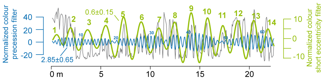
Figure 5 Colour filter outputs of short (in blue) and intermediate (green) period bands, which are related to precession couplets and short eccentricity bundles, respectively.

4.2 Detailed analysis of bundle 9 (C35–C44 interval)

4.2.1 L $/$ M ratio and calcium carbonate content

The limestone to marlstone (L $/$ M) thickness ratio of couplets varies between 0.33 (C42) and 1.36 (C39), with an average value of 0.90 (Fig. 6a, Table S2). The highest L $/$ M values are found in the couplets at the central part of bundle 9, while the lowest values correspond to couplets 41 and 42 at the boundary between bundles 9 and 10.

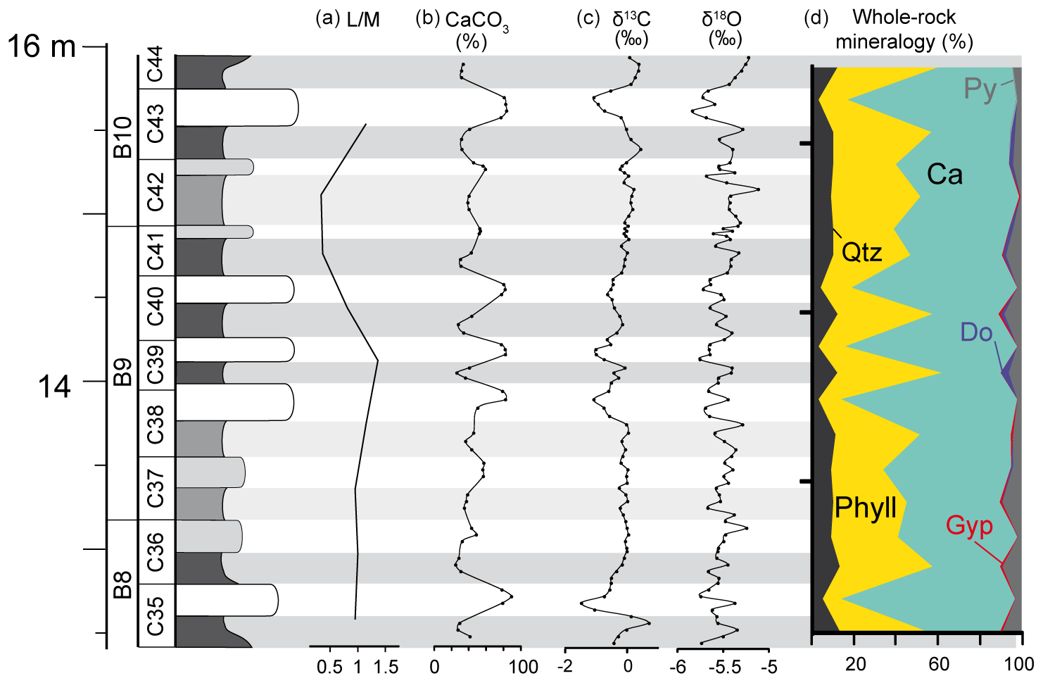
Figure 6 Lithological log of the Santiurde interval studied in detail (dark grey: shale; intermediate grey: marl; light grey: marly limestone; white: limestone), showing (a) the limestone–marl (L $/$ M) thickness ratio of couplets, (b) %CaCO₃ content, (c) δ¹³C_carb and δ¹⁸O_carb curves, and (d) whole-rock mineralogy. Numbered couplets and bundles are labelled C and B, respectively.

The CaCO₃ content ranges from 24.63 % to 88.97 %, averaging 49.78 % (Fig. 6b; Table S3). In general, %CaCO₃ fluctuates in line with the visually defined lithology, with limestone and marly limestone beds being richer in %CaCO₃ (average: 66.36 %) than marls and shales (average: 34.86 %). Marls and shales differ by 10 %–15 % in their CaCO₃ content, whereas limestone beds at the central part of bundle 9 show 20 %–40 % more CaCO₃ than marly limestones at bundle boundaries.

4.2.2 Carbon and oxygen isotopes

δ¹³C_carb values range from −1.5 ‰ (C35L) to 0.70 ‰ (C35M) and average −0.25 ‰ (Fig. 6c). The δ¹³C_carb curve shows lower values in limy beds and higher values in shales and marls. The amplitude of the fluctuations is significantly greater in the central couplets of bundle 9. δ¹⁸O values range from −5.84 ‰ (C43L) to −5.25 ‰ (C36L) and average −5.52 ‰, with the δ¹⁸O curve being rather spiky. δ¹³C_carb and δ¹⁸O_carb data show intermediate positive correlation (r: 0.53; p<0.005; Fig. S5a; Table S3).

4.2.3 General mineralogy

XRD results (Fig. 6d; Table S2) show that calcite is the most abundant mineral in limy beds and in some of the marl and shales (28 % to 84 %, average: 54 %). Clay minerals constitute the second most abundant phase (9 % to 50 %, average: 32 %), followed by quartz (3 % to 13 %, average: 9 %) and other minor components (pyrite, gypsum, and dolomite).

The mineralogical content fluctuates in line with lithology, as it shows maximum values of clays and quartz, and minima of calcite, in marls and shales. Moreover, the amplitude of the detrital–carbonate mineralogical oscillations increases in the central couplets of bundle 9. Pyrite, despite being a minor component (0.5 % to 9 %, average: 4 %), also oscillates with lithology, presenting maximum values in marls and shales, but does not match the amplitude variation associated with the bundle arrangement.

4.2.4 Organic matter geochemistry

The content in organic carbon varies between 0.26 % (C39L) and 4.03 % (C41M) (average of 1.91 %), with maximum values being found at black shales. Organic nitrogen also covaries with lithology, with values ranging from 0.02 % (C39L) to 0.09 % (C36M) (average of 0.06 %). Both elements show high-amplitude oscillations at the central part of bundle 9 and subdued oscillations at bundle boundaries. The relationship between the two organic components was calculated by the C $/$ N ratio (Fig. 7; Table S2)

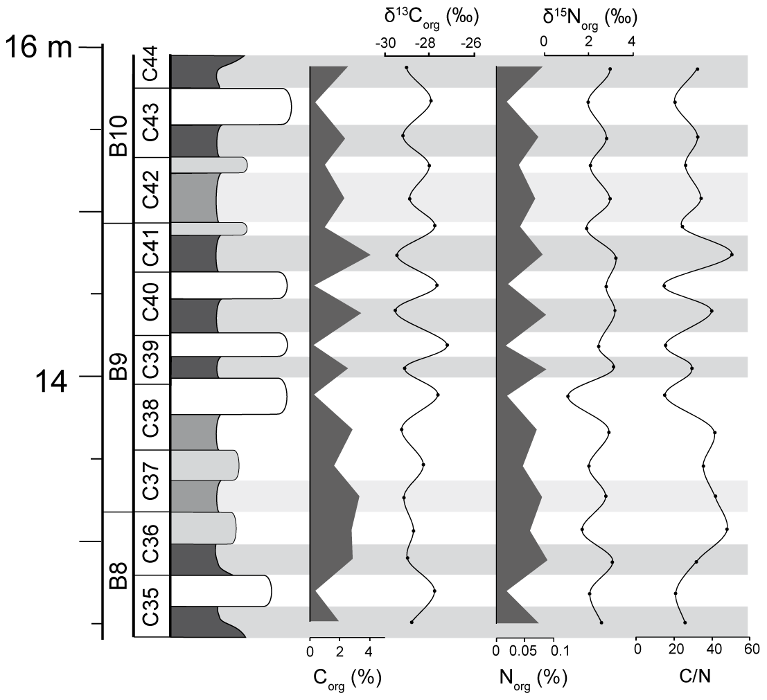
Figure 7 Lithological log of the Santiurde interval studied in detail, showing fluctuations in the percentage of organic C and N, C $/$ N ratio, δ¹³C_org, and δ¹⁵N_org.

δ¹³C_org values vary between −29.6 ‰ (C40M) and −27.2 ‰ (C40L) and average −28.6 ‰. δ¹⁵N_org ranges from 1.1 ‰ (C38L) to 3.2 ‰ (C40M), with an average value of 2.5 ‰ (Fig. 7). Both data series alternate in line with lithology, but with opposite trends. The δ¹³C_org fluctuations at the central couplets of bundle 9 show the greatest amplitude.

4.2.5 Elemental geochemistry

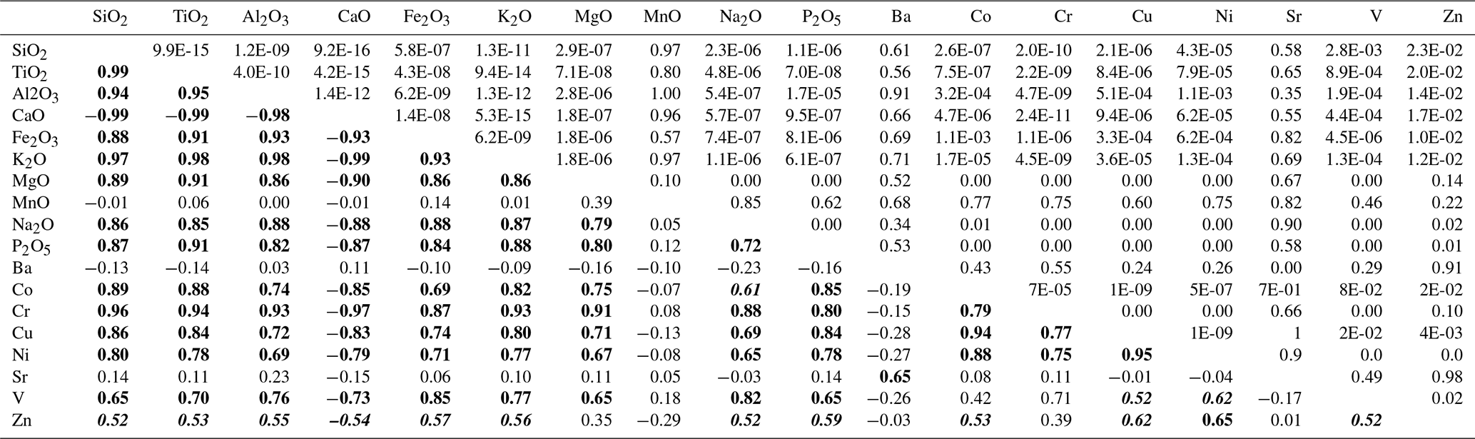
The average abundance of major and trace elements is shown in Fig. 8 (Table S4). SiO₂, Al₂O₃, and CaO constitute 48 % of limestones and 63 % of marls and shales. Average values of most major and trace elements are higher in marls and shales than in limy beds, the exceptions being CaO, MnO, Ba, and Sr. The correlation matrix shows that the abundance of MnO does not correlate with any major and trace elements, but all the other major elements present strong negative correlation (>−0.88) with CaO (Table 1) and high positive correlation with most redox-sensitive trace elements (Co, Cu, Ni, V, and Zn); the only exception is Zn, which shows intermediate positive correlations. Sr and Ba display intermediate positive correlation with each other.

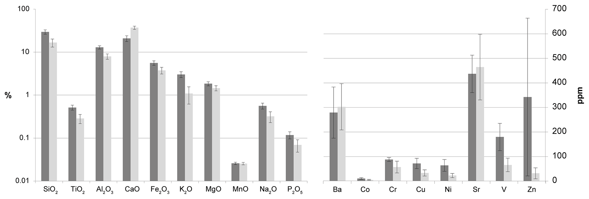
Figure 8 The average abundance of major and trace elements of limestones (pale grey) as well as marl and shales (dark grey).

Table 1 Pearson correlation coefficient (r) of major and trace element concentrations in the lower left part of the matrix. The p value for each coefficient is located in the upper right part of the matrix. The highest ($r\ge \pm \mathrm{0.65}$) correlations are marked in bold and intermediate correlations ($r=\pm \mathrm{0.50}$–0.64) in bold and italics.

In order to compare the abundance of some elements with the reference average shale composition (Li and Schoonmaker, 2003), enrichment factors (X_EF; Tribovillard et al., 2006) were calculated as follows: X_EF = (X $/$ Al)_sample $/$ (X $/$Al)_{average shale}. Al and K are commonly thought to be related to the clay fraction, whereas Si and Ti are often associated with the coarser fraction of quartz and heavy minerals (Calvert and Pedersen, 2007). Enrichment in Ti has also been related to stronger aeolian input (Rachold and Brumsack, 2001). In Santiurde K_EF, Ti_EF, and Si_EF covary with lithology, showing maximum values in marls and shales and increasing amplitude of variability in the middle part of bundle 9 (Fig. 9).

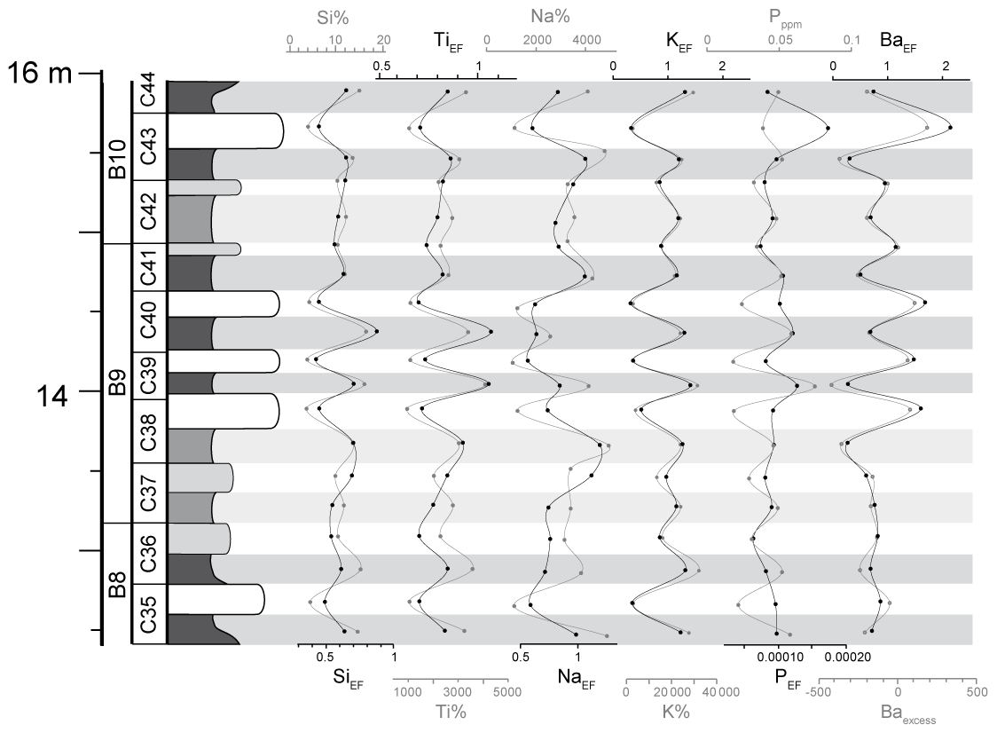
Figure 9 Lithological log of the Santiurde interval studied in detail, showing fluctuations in the percentage of elements related to detrital input (Si, Ti, Na, and K), palaeoproductivity (P and Ba), and their enrichment factors (EFs). The Ba_excess ratio is also presented.

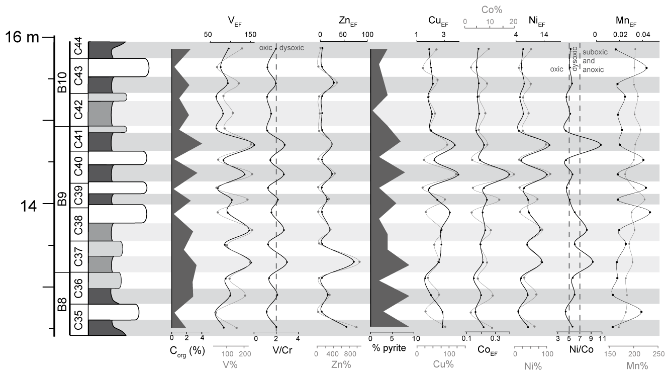
Figure 10 Lithological log of the Santiurde interval studied in detail, showing fluctuations in the percentage of redox-sensitive elements, their EFs, and several bi-elemental ratios, along with the organic carbon and pyrite content.

Marine palaeoproductivity is commonly associated with algal growth, which varies with the availability of macro-nutrients, such as P and N (Calvert and Pedersen, 2007). P_EF values from Santiurde show that these deposits are depleted in P (Li and Schoonmaker, 2003). However, P_EF shows higher values in marls and shales than in limy beds in almost all couplets (except in C35L and C43L; Fig. 9). Authigenic Ba in marine sediments is commonly associated with barite and its abundance is generally determined by organic C export from surface water into deep-marine environments (Tribovillard et al., 2006). In order to minimize the influence of detrital barium in palaeoenvironmental analyses, Ba_EF and the Ba_excess index are widely used (Dymond et al., 1992). Ba_EF shows that the studied succession is significantly depleted in Ba in comparison with average shales (Fig. 9, Li and Schoonmaker, 2003). Both Ba_EF and Ba_excess reveal increased accumulation of Ba when OM-poor limestones were deposited, which is just the opposite of P_EF.

Mn_EF is commonly linked to authigenic Mn phases, such as authigenic oxyhydroxides. In Santiurde Mn_EF shows an oscillatory pattern in line with lithology, with maximum values at limestones (Fig. 10). As no evidence of Pliensbachian hydrothermal or volcanic activity has been reported to date in the area, the higher Mn_EF in limestones could suggest increased terrestrial input, more oxygenated deep water, or increased remineralization of organic matter (Bayon et al., 2004; Tribovillard et al., 2006; Calvert and Pedersen, 2007). Both V and Zn commonly show a strong association with OM content (Calvert and Pedersen, 2007; Algeo and Liu, 2020). The type of organic matter affects the distribution of both elements, as V is taken up by tetrapyrrole complexes derived from chlorophyll decay, whereas Zn is known to be incorporated into humic and fulvic acids (Lewan, 1984; Aristilde et al., 2012). Enrichment factors of both elements show oscillatory patterns in line with lithology, with maximum values at shales and marls and a significant enrichment in V (Fig. 10). On the other hand, Co, Cu, and Ni are known to be related to sulfide fractions (Tribovillard et al., 2006; Algeo and Liu, 2020), as these elements are usually incorporated as minor constituents in diagenetic pyrite (Berner et al., 2013). With the exception of Cu_EF, the enrichment factors of these elements also fluctuate with the lithological alternation, showing maximum values in shales and marls (Fig. 10).

Several bi-elemental ratios associated with redox conditions during sedimentation were also calculated. According to absolute values of the V $/$ Cr bi-elemental ratio, most marls and shales were deposited under dysoxic conditions, whereas limestones and marly limestones accumulated in oxic conditions (Fig. 10; Jones and Manning, 1994). Ni $/$ Co values from marls and shales support dysoxic or even suboxic–anoxic conditions (Fig. 9, Jones and Manning, 1994) but suggest that limestones and marly limestones also accumulated in nearly dysoxic conditions. The discrepancy between V $/$ Cr and Ni $/$ Co results confirms the limitation of these bi-elemental ratios to discriminate absolute redox conditions (Algeo and Liu, 2020). In Santiurde all lithologies are enriched in V, Zn, Ni, and Cu when compared with average shales (Li and Schoonmaker, 2003). The concentration of these redox-sensitive trace elements is generally higher than in crustal rocks when sediments accumulate under oxygen-depleted conditions (Brumsack, 1986; Arthur and Dean, 1991). Consequently, it is assumed that deep-water oxygen concentrations were fluctuating, but the general background conditions of the environment were depleted in oxygen.

4.2.6 Factor analysis

A statistical factor analysis was conducted in order to identify key groups of variables with similar trends in the mineralogical and geochemical databases. As the number of variables introduced in the analysis has to be lower than the number of cases (19 samples), the dataset had to be reduced to 18 variables. To this end, variables with no quantifiable concentrations throughout the studied section (e.g. gypsum and dolomite content) were excluded. Elements with very strong mutual correlation coefficients (for example, Mg and Fe with Al) were also ignored because they would yield redundant data and increase the size of the dataset. Main redox-sensitive elements, in which Santiurde is enriched, have been included because of their palaeoenvironmental significance. Thus, the analysed dataset consists of 18 variables (see Table S5 and Fig. 11) from 19 cases (beds).

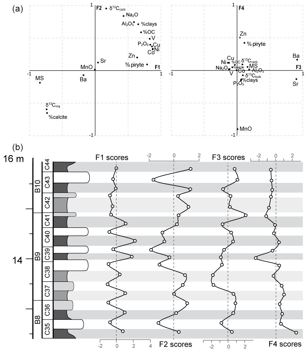
Figure 11 (a) Projection of different elements in the factor 1 versus factor 2 cross-plot (ca. 70 % of the total variance) and in the factor 3 versus factor 4 cross-plot (ca. 18 % of the total variance). (b) Stratigraphic distribution of factorial scores of the four extracted factors (virtual variables).

The optimal factor analysis (varimax rotation) extracted four factors (F1 to F4) or virtual variables that have eigenvalues greater than 1. These factors explain 87.97 % of the cumulative variance of the analysed data matrix (Fig. 11 and Table S5). Factors 1 and 2 explain the highest percentage of the dataset: 44.54 % and 25.78 %, respectively. Both factors explain the variance of variables linked to the lithological alternation and the arrangement of couplets in bundles (Fig. 11). F1 shows higher loadings for variables linked to oxygenation state (trace elements, pyrite, C_org vs. δ¹³C_org, MS) and palaeoproductivity (P₂O₃). Conversely, F2 has higher loadings in variables (Na₂O, Al₂O₃, clay% vs. calcite) linked to the dilution of calcite with terrigenous material; δ¹³C_carb also shows a very high positive loading with F2. Factors 3 and 4 explain a significantly lower variance of the total dataset: 9.92 % and 7.73 %, respectively. F3 shows very high positive loadings for Ba and Sr, whereas F4 shows very high negative loadings for MnO and intermediate positive loading for Zn and pyrite. The scores of factors 3 and 4 do not align with the lithological arrangement in couplets and bundles, which suggests that they were not controlled by the same mechanisms that produced the calcareous rhythmites.

5 Discussion

5.1 Origin of the sedimentary fluctuations

5.1.1 Santiurde rhythmites: primary or diagenetic?

Previous studies have shown that the formation of calcareous rhythmites can be caused by both primary and diagenetic processes. In some cases, rhythmites have been considered to be primary, being related to secular variations in the environmental conditions that controlled sedimentation (e.g. Arthur and Dean, 1991; Hinnov and Park, 1999; Dinarés-Turell et al., 2018; Martinez-Braceras et al., 2023). In other cases, post-depositional dissolution–cementation processes have been considered the most important (e.g. Hallam, 1986; Reuning et al., 2002; Westphal, 2006; Nohl et al. 2021). When differential diagenesis affects the primary composition of sediments, part of the carbonate dissolves from marly beds and migrates to limy beds, precipitating as cements (Westphal, 2006).

The aragonitic and high-Mg calcite components of limestones, including their micritic matrix, suffered significant recrystallization. However, none of the limestone beds display a nodular geometry, which is common in successions affected by intense post-depositional dissolution–cementation processes (Hallam, 1986; Einsele and Ricken, 1991). Quite the opposite, the characteristics of the beds are continuous for more than 1 km, as shown by bed-by-bed correlation between the Santiurde section studied herein and the railway section studied by others (Rosales et al., 2001, 2004, 2006; Quesada et al., 2005; Fig. S1). Furthermore, petrographic and SEM observations suggest that fluid migration from marly to limy beds was overall limited. Thus, skeletal components of marls and shales (Figs. 2 and 3) do not present features of increased compaction (Munnecke et al., 2001; Westphal, 2006). This was probably related to an original higher clay content in marls and shales, which hampered fluid migration between beds and prevented intense dissolution and recrystallization. In addition, clay minerals show primary textures (such as deformed, broken plates or isolated flakes wrapping other detrital grains) but do not show any evidence of intense diagenetic recrystallization.

Interestingly, the lithological arrangement in couplets and bundles observed in the outcrop, combined with the spectral analysis of colour and MS data series, highlights the presence of sedimentary cycles with three main periodicities in the succession (6.6 : 1.67 : 0.36). This ratio is comparable to the 405 : 100 : 20 ratio produced by the superposition of long eccentricity, short eccentricity, and precession cycles (Berger and Loutre, 1994). Unfortunately, the available chronostratigraphic framework (Braga et al., 1988; Fraguas et al., 2015) does not provide the resolution required to confirm the duration of the sedimentary cycles.

The abovementioned characteristics strongly suggest that the formation of the Santiurde rhythmites was primary and responded to orbitally driven climate change episodes. An orbital control on sedimentation had previously been deduced in other Pliensbachian successions from nearby areas, such as the Asturian and Iberian basins (Bádenas et al., 2012; Val et al., 2017; Sequero et al., 2017).

5.1.2 Preservation of the geochemical signal

Although the formation of the Santiurde rhythmites was a result of orbitally paced environmental variations, some primary sedimentary characteristics (such as chemical and mineralogical composition, fossil assemblage, or porosity) could have responded in different ways to diagenesis. Consequently, the geochemical data for the seven limestone–marl couplets (C35–C44) studied in detail must be analysed carefully in order to interpret which environmental variations controlled sedimentation.

Whole-rock inorganic isotopic analyses from diagenetically “closed” systems, such as hemipelagic carbonates, have been used successfully for the climatic reconstruction of ancient sedimentary environments (e.g. Jenkyns and Clayton, 1986; Marshall, 1992; Silva et al., 2011; Martínez-Braceras et al., 2017; Deconinck et al., 2020). However, δ¹³C_carb and δ¹⁸O_carb values tend to get depleted during burial, causing a significant positive correlation between them when strong deep burial diagenesis affects the succession (Banner and Hanson, 1990; Marshall, 1992; Swart, 2015). In Santiurde both isotopic records show depleted values in comparison to Early Jurassic marine isotopic standard curves (Grossman and Joachimski, 2020; Cramer and Jarvis, 2020). Both δ¹⁸O_carb and δ¹³C_carb records show a positive but not very high correlation (Fig. S5a; r: 0.53, p<0.005), following a common burial trend (Banner and Hanson, 1990). This suggests that, although primary isotopic trends may have been preserved, absolute values are probably distorted. Accordingly, δ¹⁸O_carb values from Santiurde are significantly depleted (Grossman and Joachimski, 2020) and display a spiky curve (Fig. 6). This may reflect the impact of the percolation of diagenetic fluids in post-depositional processes at low fluid $/$ rock ratios (Banner and Hanson, 1990). Consequently, δ¹⁸O_carb values were only used to assess the degree of diagenetic overprinting.

Rosales et al. (2001) concluded that whole-rock stable isotope records from the Jurassic hemipelagic carbonates of the BCB are not suitable for accurate palaeoceanographic reconstructions because their high OM content contributed to the alteration of their primary signal. In fact, organic matter degradation and sulfate reduction in deep-sea sediments are known to produce CO₂ enriched in ¹²C and generate early cements with low δ¹³C_carb (Dickson et al., 2008; Swart, 2015). Accordingly, the generally depleted δ¹³C_carb values in Santiurde could be a consequence of the addition of early cements precipitated in equilibrium with isotopically light pore water affected by OM decay. This process, however, cannot explain the δ¹³C_carb fluctuations observed along the lithological alternation because the influence of δ¹³C-depleted fluids is generally thought to be more pronounced when carbonate content in the sediment is low and the total organic carbon is comparatively high (Ullman et al., 2022). Contrarily, in Santiurde maximum δ¹³C_carb values are recorded in marls and shales, and the cross-plot of δ¹³C_carb versus CaCO₃ values shows a high negative correlation (r: −0.75, p<0.005; Fig. S5b). It can therefore be assumed that the high clay content and low porosity in marls and shales probably hampered a more intense cementation during early diagenesis (Arthur and Dean, 1991).

Additionally, dissolution of aragonite and high-Mg calcite components, which are generally more abundant in shallow marine areas, and precipitation of more stable low-Mg calcite phases are important post-depositional processes causing carbon isotope fractionation (Reuning et al., 2002). Aragonite is generally characterized by more positive δ¹³C values than high- or low-Mg carbonates (Swart, 2015). Therefore, a fluctuating rate of aragonitic input could produce covarying δ¹³C_carb and %CaCO₃ records (Reuning et al., 2002), like that found in Santiurde. However, given that minimum δ¹³C_carb values are found at %CaCO₃ maxima in Santiurde, the carbonate distribution does not record variations in the supply of platform-derived fine-grained aragonitic and high-Mg calcite.

Whole-rock δ¹³C and δ¹⁸O average values similar to those obtained in Santiurde were also found in the coeval Rodiles hemipelagic section from the Asturian basin (Deconinck et al., 2020), with that isotopic trend being considered to reveal primary environmental changes. Taking everything into account, it can be concluded that the δ¹³C_carb record from Santiurde may reflect the original isotopic composition of seawater, but the possibility cannot be excluded that the fluctuations respond to variations in the rate of recrystallization. However, the elemental geochemical evidence further suggests that, in addition to the original composition and porosity of the different layers, the Santiurde rhythmites also record variations in the supply of terrigenous components. Thus, diagenetically inert trace elements, such as Ti_EF, also show variations in line with the lithological alternations (Nohl et al., 2021).

Other elements, such as Sr, Fe, and Mn, are sensitive to burial and may be used to assess the degree of diagenetic overprinting in carbonates in combination with δ¹⁸O_carb values (Marshall, 1992; Rosales et al., 2001; Zhao and Zheng, 2014). In general, during diagenesis, marine carbonates tend to become depleted in Sr and δ¹⁸O but enriched in Fe and Mn (Banner and Hanson, 1990). There is no correlation between the abundance of these three elements in Santiurde (Fig. S6; Sr–Mn r: 0.03, p: 0.9; Sr–Fe r: 0.06, p: 0.82; Mn–Fe r: 0.14, p: 0.58). Moreover, δ¹⁸O_carb values do not display any correlation with Sr and Mn and show positive correlation with Fe, which is just the opposite of what should be expected from post-depositional distortion. Similarly, when compared with the average shale composition (Li and Schoonmaker, 2003), both limestones and marls from Santiurde are significantly enriched in Sr (402.5 ppm), slightly enriched in Fe (32 750 ppm), and depleted in Mn (199 ppm). Taking everything into account, a strong diagenetic overprinting can be ruled out.

In conclusion, burial diagenesis produced depleted inorganic stable isotope values, but there are no signs of strong differential diagenesis or post-depositional redistribution of geochemical components in the Santiurde section. The δ¹³C_carb signal was affected by early diagenetic processes related to OM decay in limestones but not to the extent of obscuring the original fluctuating trend.

5.2 Fluctuations in OM content

Detailed multiproxy analysis carried out throughout seven limestone–marl couplets from the oldest BSI cast light on the origin of OM and the sedimentary factors that controlled its distribution. Rosales et al. (2006) showed that BSIs accumulated during second-order sea level rises, which produced the flooding of large continental areas and the creation of a moderately isolated epicontinental sea, in which water circulation was relatively restricted. More specifically, sluggish circulation at the depocentres of the irregular floor of the BCB contributed to increasing density stratification of the water column and caused a sea floor depleted in oxygen (Wignall, 1991; Quesada et al., 2005), which prevented oxidation of the high organic matter content of the section.

In Santiurde, the OM content fluctuates in line with lithology, suggesting that the environmental factors that controlled its accumulation and/or preservation varied cyclically (Fig. 7). The fluctuations in OM content could be the result of variations in either the flux of organic matter to the sea floor (i.e. fluctuations in productivity), the rate of dilution by terrestrial or carbonate sedimentary inputs, or the rate of organic matter remineralization (i.e. fluctuations in preservation) due to changing seawater oxygen concentrations (Tyson, 2005; Swart et al., 2019). The greatest part of the organic matter found in the BCB Pliensbachian black shales had a marine origin (see Appendix A; Suárez-Ruiz and Prado, 1987; Quesada et al., 1997, 2005; Permanyer et al., 2013).

Many factors affect sedimentary δ¹³C_org values of marine sediments, such as biological sources, recycling of organic matter, and marine productivity (e.g. Nijenhuis and Lange, 2000; Tyson, 2005; Meyers et al., 2006; Luo et al., 2014). Changes in marine productivity can be ruled out for the Santiurde δ¹³C_org fluctuations. Indeed, increased OM production generally results in greater sequestration of ¹²C, which would lead to higher δ¹³C_org values when OM content increased (Meyers et al., 2006); this is just the opposite of the Santiurde trend (Fig. 7). This is also confirmed by δ¹⁵N_org values, which can also be subject to fractionation due to variations in productivity. N is assimilated by organisms in order to produce biomass, preserving the δ¹⁵N_org value of its source. Marine δ¹⁵N_org values are influenced by changes in ocean circulation, the strength of biological pump, large-scale N cycling, and redox conditions (Robinson et al., 2012). However, δ¹⁵N_org values may also be subject to alterations during sedimentation, burial diagenesis, catagenesis, and hydrocarbon migration (Robinson et al., 2012; Quan and Adeboye, 2021). Average δ¹⁵N_org values from Santiurde (Fig. 7) are close to the current ocean isotopic ratio (∼5 ‰; Robinson et al., 2012) and vary within the range observed in other organic-rich sediments and rocks (principally shales and marlstones; Holloway and Dahlgren, 2002). Increased N fixation rates have been observed in episodes of increased nutrient supply modulated by precession cycles (Higginson et al., 2003; Swart et al., 2019). In such cases, low δ¹⁵N_org values coincide with increased primary productivity and OM accumulation, which is just the opposite of the relationship found in Santiurde. Alternatively, in other marine records, the shallow-water δ¹⁵N_org signal suffered fractionation due to the liberation of bottom water enriched in ¹⁵N_org (upwelling systems; Altabet et al., 1995). In those cases, marine productivity increased due the liberation of nutrients stored in the sea bottom and more OM with a relatively higher δ¹⁵N_org signal was produced. However, the restricted palaeogeographic setting and the sedimentary features preserved (absence of phosphatic and glauconitic deposits) do not support the influence of upwelling currents in Santiurde.

Average P_EF values from Santiurde are relatively depleted in P (Li and Schoonmaker, 2003), but the P content, as well as the P_Ef record in almost all couplets, displays a fluctuating trend with maxima at OM-rich marls and shales (Fig. 9). Greater accumulation of P in marls and shales suggests that OM might have increased due to enhanced marine productivity (Calvert and Pedersen, 2007). Although Ba-related indexes would not support this interpretation, authigenic barite dissolves when bottom-water oxygenation is limited (Dymond et al., 1992; Tribovillard et al., 2006). Consequently, it is possible that the Ba content does not reflect palaeoproductivity ratios. Although P_EF data support a relationship between greater OM accumulation and higher palaeoproductivity (Tribovillard et al., 2006; Swart et al., 2019), a more comprehensive palaeoecological study should be carried out in order to support this interpretation.

Fluctuations in the rate of dilution of OM by non-organic components can also result in an alternation of organic-rich and organic-poor beds (Bohacs et al., 2005). In Santiurde C_org and phyllosilicate contents show a strong positive correlation (r: 0.82; p<0.005; Fig. 12a) and covary in line with the rhythmites. This shows that C_org oscillations were not caused by variations in the rate of dilution by clays. The CaO–Al₂O₃–C_org ternary plot (Fig. 12c) also illustrates that the C_org $/$ Al₂O₃ ratio is relatively constant, whereas higher variability is observed in the CaO $/$ Al₂O₃ and C_org $/$ CaO ratios. Therefore, C_org fluctuations could have resulted from cyclic variations in the dilution rate by calcite input. In fact, the cross-plot between calcite and C_org shows a strong negative correlation (Fig. 12b; r: −0.83; p<0.005), which is typical of dilution-driven OM fluctuations (Arthur and Dean, 1991; Beckmann et al., 2005). In order to disentangle the origin of the cyclic sedimentation, bed thickness and duration must be taken into consideration (Einsele and Ricken, 1991). If variations in the rate of carbonate sedimentation had been the only process controlling organic matter dilution, while OM and clay mineral inputs stayed constant, limestone beds would have been significantly thicker than marls and shales, which is not the case in Santiurde (Fig. 6a). This suggests that a greater input of clay minerals must have also occurred during the deposition of marls and shales. Moreover, marls and shales display greater dispersion in the C_org vs. calcite cross-plot (Fig. 12b), which suggests that there might have been other factors controlling OM content, such as changes in OM production or preservation (Bohacs et al., 2005).

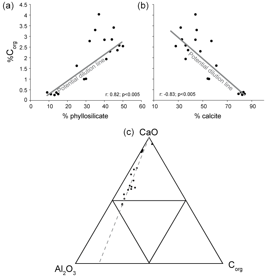
Figure 12 Cross-plot of C_org against (a) phyllosilicate and (b) calcite content. Potential dilution lines of C_org are marked in both graphs. (c) Ca–Al–C_org ternary plot with Santiurde samples, which follow a constant C_org $/$ Al₂O₃.

Accordingly, the sedimentological and geochemical evidence strongly suggests that the fluctuations in OM content were closely related to variations in the rate of organic matter remineralization (preservation) as a consequence of secular variations in seawater oxygen concentrations. The well-preserved lamination, the absence of burrows, and the scarcity of benthic fauna (Figs. 2 and 3) of shales strongly suggest that the sea floor was depleted in oxygen. Conversely, bioturbation structures and benthic fauna are more diverse and abundant in limestones, suggesting better oxygenation of the seabed (Figs. 2 and 3). Changing redox conditions can also be deduced from δ¹³C_org records (Algeo and Liu, 2020). Microbial chemoautotrophy, which is typical of oxygen-depleted environments, fixes carbon enriched in ¹²C, producing lower δ¹³C_org values than OM produced by photosynthetic eukaryotic algae (Nijenhuis and Lange, 2000; Luo et al., 2014). Accordingly, minima in δ¹³C_org from OM-rich marls and shales from Santiurde are very likely related to reducing deep-water conditions, similar to those deduced for some Pliocene sapropels (Nijenhuis and Lange, 2000). The strong negative correlation between C_org content and δ¹³C_org (r: −0.945, p<0.0001) supports the close relationship between seabed oxygenation conditions and OM preservation. This interpretation is in line with that derived from the abovementioned C $/$ N ratio (Appendix A), which also suggests that denitrification intensified during deposition of marls and shales due to more reducing sea-bottom conditions.

The interpretations above are also supported by N_org and δ¹⁵N_org data. Denitrification can result in δ¹⁵N_org isotope fractionation in poorly oxygenated conditions, as denitrification and anaerobic ammonium oxidation reactions increase ¹⁵N_org in OM (Robinson et al., 2012). In Santiurde δ¹⁵N_org isotopes fluctuate in line with the lithological rhythmites (Fig. 7), showing maxima at marls and shales and hence a significant negative correlation with δ¹³C_org (r: −0.70p<0.005) and positive correlations with C_org (r: 0.66, p<0.005) and N_org (r: 0.73, p<0.005) content. It can therefore be concluded that δ¹⁵N_org values increased during the accumulation of marls and shales, when bottom-water oxygenation decreased and denitrification intensified.

Pyrite and C_org contents also show an intermediate positive correlation in Santiurde (r: 0.6, p<0.01). Pyrite might be formed during very early diagenesis due to reactions between Fe and H₂S. H₂S is generally released into porewater when sulfate-reducing bacteria use sedimentary organic matter as a reducing agent and energy source (Berner, 2013). More oxygenated conditions during the deposition of limestones could have inhibited the formation of pyrite. Conversely, limestones present higher MS values than marls and shales, possibly associated with a greater concentration of magnetite (Fig. S3). Magnetite could be either detrital in origin or related to post-depositional changes in redox state, as more oxygenated conditions favour the partial replacement of pyrite with iron oxides, such as magnetite (Lin et al., 2021).

Finally, the correlation matrix (Table 1) and the factor analysis (Fig. 11) also show a close relationship between some redox-sensitive elements (Fig. 10; V, Zn, Co, Cu, Ni), pyrite, and C_org content (Calvert and Pedersen, 2007; Algeo and Liu, 2020). Enrichment factors and ratios highlight a relative enrichment in redox-sensitive elements throughout the succession, which supports the general depositional model of a sea floor depleted in oxygen (Quesada et al., 2005; Rosales et al., 2006). Trace-metal enrichment factors and bi-elemental ratios associated with both sulfides and organic matter vary in line with the lithological rhythmites and support the interpretation of alternating environmental redox conditions.

To sum up, the multiproxy analysis (δ¹⁵N_org, δ¹³C_org, trace elements, mineralogy, and sedimentology) shows that the higher C_org content in marls and shales was related to less oxygenated sea floor conditions, which enhanced the preservation potential of organic matter. The P_EF record suggests that the production of organic matter may have also increased during the formation of marls and shales, but this signal is not coherent throughout the studied interval. Given the close relationship between these processes and the lithological rhythmites, it can be concluded that there must have been an orbitally driven environmental factor that triggered fluctuations in bottom-water oxygenation and, possibly, palaeoproductivity.

5.3 Orbitally modulated environmental changes

Previous studies of northern Iberian Pliensbachian records have demonstrated that this area was subject to semiarid climatic conditions, with physical erosion being prevalent in the continent and seawater being temperate (Rosales et al., 2004; Armendáriz et al., 2012; Gómez et al., 2016; Deconinck et al., 2020). The BCB, being located close to the boundary between the arid and humid climatic belts at approximately 30° N palaeo-latitude, was especially sensitive to orbitally driven climate change episodes, which were recorded by the outer-ramp hemipelagic rhythmites from Santiurde. These rhythmites are best characterized in the stratigraphic succession by decimetre-scale calcareous couplets, which represent precession cycles, and metre-scale bundles linked to short eccentricity cycles. The imprint of long eccentricity cycles can also be identified in the field and deduced by spectral analysis (Fig. 4). Based on the number of orbital cycles found in Santiurde (62 precession couplets and 13.4 short eccentricity bundles) and the average duration of 20 kyr for precession cycles and 100 kyr for short eccentric cycles, the studied succession has an estimated duration of 1.29±0.05 Myr and the BSI-1 interval of 750±30 Myr (36 precession couplets and 7.8 short eccentricity bundles).

5.3.1 Formation of precession-driven calcareous couplets

The sedimentary processes behind the formation of precession couplets can be analysed on the basis of thickness relationships between the constituent lithologies (Einsele and Ricken, 1991). When limy beds are thicker than marly beds, the formation of calcareous couplets is commonly attributed to fluctuations in either carbonate dissolution or carbonate production. Contrarily, marls and shales are usually thicker than limestones when periodic changes in the rate of dilution by terrigenous components originate the couplets. Periodic carbonate dissolution can be ruled out in Santiurde, as there is neither macroscopic nor microscopic evidence of pervasive carbonate dissolution and the outer-carbonate-ramp seabed was permanently above the carbonate compensation depth (Bjerrum et al., 2001). The L $/$ M ratio is close to 1 in most of the couplets (Fig. 6a). Consequently, the formation of the Santiurde precession-driven couplets most likely responded to periodic changes in both carbonate production and carbonate dilution by terrigenous material, increasing accumulation and preservation of C_org when marls and shales were deposited. In fact, factor analysis points out that precession-driven lithological alternation (Fig. 11) is strongly associated with redox-sensitive variables and terrigenous proxies.

Given the generally semiarid Pliensbachian conditions deduced for the BCB (Dera et al., 2009; Deconinck et al, 2020), a climate characterized by a prolonged dry season and a short wet season can be envisaged. Dry sub-humid climates, with 3 to 5 wet months per year and a maximum degree of seasonality, produce maximum values of fluvial sediment discharge into the sea (Cecil and Dulong, 2003). Such high seasonality conditions are generally produced when the precessional configuration results in summers occurring at perihelion and winters at aphelion (Fig. 13). In Santiurde both the L $/$ M ratio and the terrigenous content of couplets suggest that shales and marls were formed in such an astronomical configuration. Intensified monsoons during the wet season could have increased the fluvial discharges that reached periplatform areas, producing maxima of geochemical proxies associated with coarser detrital grain size, such as Si_Ef or Ti_EF (Fig. 9; Calvert and Pedersen, 2007). However, inorganic and organic stable isotope records do not support an increased input of fresh water or terrestrial OM when marls and shales were deposited. Alternatively, it is also possible that the terrigenous material was transported by wind. Indeed, other studies have also related an enrichment in Si and Ti content in pelagic sediments to stronger aeolian input (Rachold and Brumsack, 2001) and increased dust production and transportation during high seasonality conditions (Woodard et al., 2011). Thus, it can be assumed that dust generation increased in the continents near Santiurde during extremely dry seasons at precessional configurations leading to maximum seasonality. Extreme seasonality conditions may have also increased dust storms and dust input into the adjacent ocean (McGee et al., 2010). Either aeolian or fluvial, increased terrigenous input during maximum seasonality conditions may have also supplied nutrients to the ocean (P_EF), triggering organic phytoplankton blooms and organic matter production. This situation promoted greater OM accumulation and oxygen depletion in deep-sea sediments (e.g. Nijenhuis and Lange, 2000; Wang, 2009; Chroustova et al., 2021). Given that the evidence of changing palaeoproductivity is scarce, it is also possible that orbitally forced mechanisms also modulated the amount of dissolved oxygen in seawater. As there is no evidence of a great influence of continental water masses that could have prompted density stratification of the water column (e.g. Arthur and Dean, 1991; Chroustova et al., 2021), it is more likely that the mechanism was marine in origin. Interestingly, numerical simulations suggested that during the Late Cretaceous hothouse both precession and eccentricity cycles modulated seawater ventilation and oxygenation, driven by changes in deep-ocean circulation (Sarr et al., 2022). According to this model, basins that were depleted in oxygen were especially sensitive to orbitally forced ventilation variations. More specifically, the precessional configuration with the higher seasonality recorded the greatest oxygen depletion at intermediate and deep-water depths, producing a strong vertical oxygen gradient and seawater stratification. In Santiurde, similarly reduced vertical mixing may have occurred during the accumulation of marls and shales, which would have enhanced deep-water anoxia. Indeed, in Early Jurassic times, lower-frequency orbital cycles also triggered periodic changes in the ventilation and oxygenation of bottom sediments, controlling carbonate and OM accumulation (Pieńkowski et al. 2021). Thus, the southward flow of Arctic water from the Boreal Sea into the Laurasian epicontinental seaway favoured thermohaline circulation and the ventilation of deep water. However, in periods of high atmospheric CO₂, more sluggish currents or stagnant conditions prevailed due to the influx of warm and saline water from the Tethyan area. It is possible that the early Pliensbachian BCB rhythmites recorded similar, but probably weaker, palaeoceanographic changes at precession timescales. Anoxic bottom-water conditions allowed OM to be preserved, favoured the precipitation of authigenic sulfides and the dissolution of Fe and Mn oxo-hydroxides (Capet et al., 2013), and altered the organic isotopic signal (enrichment in ¹³C_org and depletion in ¹⁵N_org). Increased OM burial also resulted in a decrease in the ¹²C content of inorganic carbon dissolved in seawater (Mackensen and Schmiedl, 2019). Although the ¹³C_carb signal found in Santiurde records this C storage fractionation, it is not possible to quantify the diagenetic imprint.

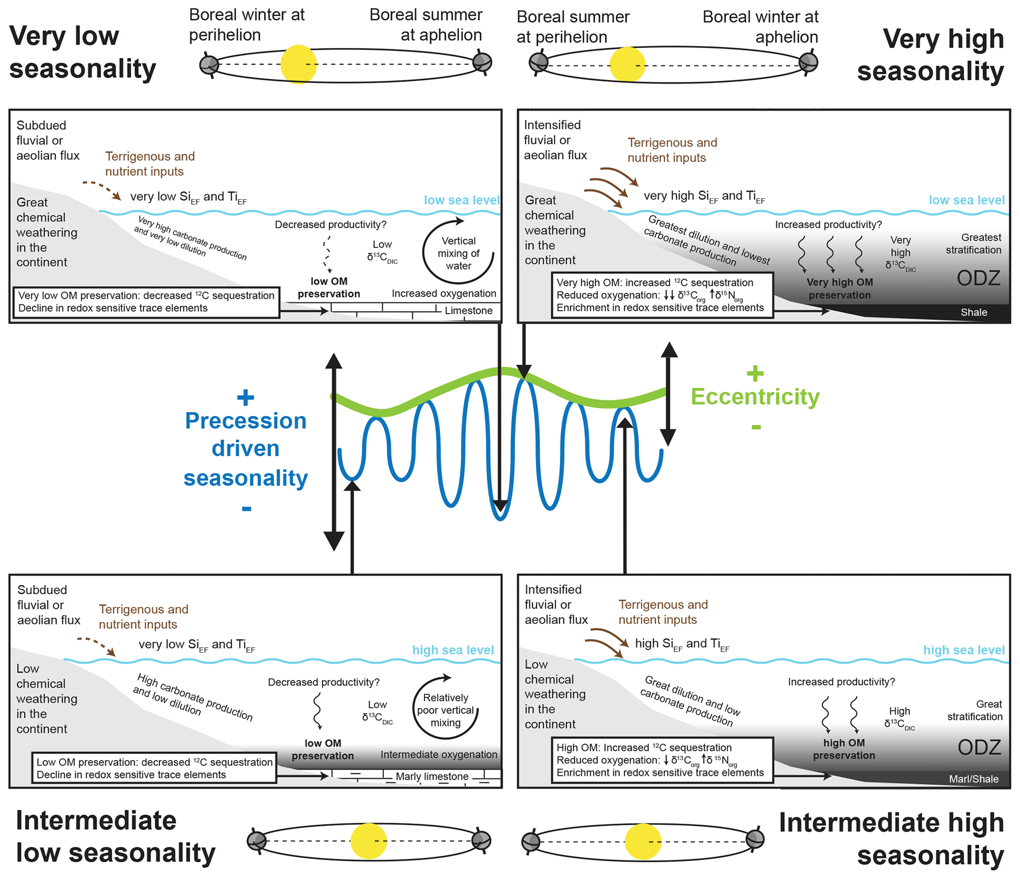
Figure 13 Orbitally tuned depositional model for the formation of the calcareous couplets and bundles from Santiurde. Schemes on the left represent environmental conditions during precessional stages with low annual seasonality (boreal summertime at aphelion). Schemes on the right represent environmental conditions during precessional stages with high annual seasonality stages (boreal summertime at perihelion). The influence of maximum eccentricity is shown at the top and that of minimum eccentricity at the bottom. DIC: dissolved inorganic carbon. ODZ: oxygen-depleted zone.

In contrast, OM-poor limy beds accumulated during low seasonality precessional stages. Such low seasonality conditions (mild summers and winters) resulted when summers occurred at aphelion and winters at perihelion (Fig. 13). Mild wet and dry seasons caused a decrease in detrital input (by wind and rivers), as well as in nutrient supply. Consequently, organic matter production and bottom-water oxygen consumption declined (e.g. Nijenhuis and Lange, 2000; Wang, 2009; Chroustova et al., 2021). Moreover, according to the orbitally modulated ocean circulation model (Sarr et al., 2022), low-seasonality precessional stages would have also favoured vertical mixing of the water column, bringing oxygen to bottom water, which allowed the oxidation of organic matter (Capet et al., 2013). Regarding carbonate components, previous studies have shown that Jurassic shelfal carbonate factories were more efficient than pelagic ooze in micrite production (Hinnov and Park, 1999; Bádenas et al., 2012). It can therefore be concluded that decreased terrigenous inputs into shallow marine areas further increased shelfal carbonate mud production, with surpluses being exported into deeper areas (Tucker et al., 2009; Bádenas et al., 2012). Assuming the general δ¹³C_carb trend to be primary, the enrichment in ¹²C of limestones could correspond to the OM balance in the marine environment (Mackensen and Schmiedl, 2019). Thus, well-oxygenated bottom water allowed most of the ¹²C-rich OM to be oxidized before burial, decreasing the δ¹³C of inorganic carbon dissolved in seawater.

The palaeoenvironmental model derived from the Santiurde precession couplets differs significantly from those presented by others for lower Pliensbachian successions from NW and central Europe (Fig. 1; Martinez and Dera, 2015; Hollar et al., 2023). However, it should be taken into account that these models were developed for successions accumulated in the humid climatic belt, where wet conditions prevailed throughout the year and seasonality was generally weak. In such settings, terrigenous and nutrient inputs increased at precessional configurations with higher seasonality, causing greater productivity during the wettest season and stronger vertical water mixing during the drier season. Consequently, the more calcareous OM-poor beds accumulated at high-seasonality precessional stages.

5.3.2 Formation of eccentricity-driven bundles

During an eccentricity cycle, the amplitude of precession-driven seasonality cycles is modulated by variations in the shape of the orbit of the Earth around the Sun (Berger and Loutre, 1994). At maximum eccentricity the orbit of the Earth is elliptical, and, consequently, insolation changes as much as 24 % in 1 single year, causing significantly contrasting seasonality conditions (Fig. 13). On the contrary, at minimum eccentricity the orbit of the Earth is almost circular, which results in relatively small variations in insolation between aphelion and perihelion, regardless of the precession-driven orientation of the axis of the Earth. In short, two extreme climatic situations (maximum and minimum seasonality) alternate throughout 20 kyr precession cycles at maximum eccentricity, whereas climatic conditions remain stable for longer periods at eccentricity minima.

In Santiurde the arrangement of couplets in bundles is the lithological expression of the modulation of the amplitude of precession-driven seasonality by eccentricity cycles (Fig. 2b). In the interval studied in detail, couplets 36–37 and 41–42, located at the boundaries between bundles 8–9 and 9–10, show relatively little lithological contrast (marls alternating with marly limestones), which suggests formation at eccentricity minima. The rest of the couplets are situated in the central parts of bundles and show a marked lithological contrast (shales alternating with limestones), which suggests formation in the two extreme situations that occur during precession cycles at maximum eccentricity. This amplitude modulation is also recorded by several geochemical and mineralogical proxies, corroborating the impact of eccentricity cycles on the formation of the rhythmite.

The fluctuations in some redox-sensitive (C_org, N_org, trace elements, δ¹³C_org, Mn_EF) and productivity (represented by P_EF) proxies, some of them associated with factor 1 in the factorial analysis (Fig. 11), display greater amplitude during eccentricity maxima. This suggests that intensified precessional seasonality at maximum eccentricity caused an increase in terrestrial sediment and nutrient input to the sea, which ultimately resulted in the intensification of OM production and oxygen consumption (e.g. Nijenhuis and Lange, 2000; Wang, 2009; Chroustova et al., 2021). Precession-driven variations in oceanic currents, which controlled vertical oxygen gradient and seawater stratification, also contributed to promoting bottom-water anoxia in this orbital configuration (Sarr et al., 2022).

Eccentricity cycles also modulated the low-seasonality precessional stages, in which carbonate accumulation was favoured (Hinnov and Park, 1999; Bádenas et al., 2012). At extremely low seasonality conditions at eccentricity maxima, continental inputs were minimal and, consequently, so was marine OM production. At the same time, oceanic currents intensified vertical mixing of water, favouring a well-oxygenated water column and carbonate production (Sarr et al., 2022). Moreover, factor 2, which comprises proxies associated with dilution of carbonate by terrigenous input, shows an interesting trend in line with eccentricity bundles. Scores of factor 2, in addition to fluctuating with the lithological alternation of calcareous couplets, also display a larger-scale trend with minimum values at eccentricity maxima and maximum values at eccentricity minima. This trend is mainly produced by Na₂O and ¹³C_carb (Table S5). Indeed, Na_EF also shows a similar trend, with generally lower values at eccentricity maxima (Fig. 9). This may record increased chemical weathering in the continent and the release of Na₂O (Marshall, 1992). This goes against the orbitally modulated climatic model of Martinez and Dera (2015), who concluded that chemical weathering increases during low seasonality and annually wet climates developed at eccentricity minima. Data from Santiurde, however, suggest that the climate was drier at eccentricity minima.

5.3.3 Orbitally paced sea level changes?

It is well known that, during icehouse periods, climate change driven by high-frequency orbital cycles affects sea level due to fluctuations in the storage of water in continental ice, causing so-called glacio-eustatic sea level changes (Steffen et al., 2010). High-frequency sea level changes have also been deduced from many shallow marine platforms developed in ice-free greenhouse periods (Haq, 2014). In the absence of extensive ice caps, sea level changes must have been caused by forcing mechanisms other than glacio-eustasy, which are still debated. The thermal expansion and contraction of water masses cause sea level changes but do not produce high-amplitude variations (Conrad, 2013). Fluctuations in water storage in continental areas (principally in aquifers) seem to be a plausible forcing mechanism of decametric sea level changes during greenhouse conditions (Wendler and Wendler, 2016). According to the aquifer–eustatic model, low sea levels occur when large volumes of water are stored in the continents during humid stages, whereas sea level rises during dry epochs due to increased aquifer discharge (Sames et al., 2020). Consequently, in a greenhouse context, orbitally driven alternations of arid and humid periods can produce third- and fourth-order sea level fluctuations (Wendler and Wendler, 2016; Sames et al., 2020). Greater accumulation of δ¹⁸O- and δ¹³C-depleted fresh water in the continent results in heavier δ¹⁸O and δ¹³C of inorganic carbon dissolved in seawater, and vice versa.

Second-order sea level changes occurred in Early Jurassic times in the BCB, which were recorded by δ¹³C in well-preserved belemnites (Rosales et al., 2006). Highstand deposits show maximum values in OM content and δ¹³C values in belemnites, while lowstand intervals are characterized by carbonate-rich sedimentation and lower δ¹³C values in belemnites. These carbon isotope records reflect fluctuations in the δ¹³C composition of the inorganic carbon dissolved in seawater, which were controlled by periodic variations in OM burial and storage of ¹²C in the seabed (Quesada et al., 2005; Rosales et al., 2006). This suggests that water stratification increased and ventilation of the seabed decreased in highstands. Martinez and Dera (2015) showed that δ¹³C values from Jurassic and Lower Cretaceous Perithetyan successions also recorded second- and third-order sea level changes modulated by orbital cycles. According to this study, flooding of continental areas at highstands triggered marine productivity, and, consequently, seawater δ¹³C values increased in neritic domains.

In Santiurde, several lines of evidence suggest that short eccentricity cycles could have modulated sea level. Factor 2 scores (Table S5) change in line with eccentricity bundles, displaying higher values at eccentricity minima and lower values at eccentricity maxima (Fig. 14). Average δ¹³C_carb, %CaCO₃, and Ti_EF values per couplet show high values at eccentricity minima. Average C_org and N_org values per couplet also fluctuate in line with eccentricity bundles, showing maximum (or minimum) values in the intervals that correspond to low-eccentricity (or high-eccentricity) configurations. This may indicate that the average OM content per precessional stage was higher at eccentricity minima, although shales at eccentricity maxima recorded maximum OM values. Using the aquifer–eustatic model, it can be postulated that low sea levels may have occurred during eccentricity maxima. Lowstand deposits recorded the highest and probably coarsest terrigenous inputs (Ti_EF; Olde et al., 2015) but also the most calcareous sedimentation due to platform progradation. A lower sea level would have facilitated seawater ventilation and OM degradation at eccentricity scale. However, ventilation at maximum eccentricity decreased when precession-driven seasonality increased, which temporarily enhanced OM production and preservation, and caused the accumulation of shales on the seabed. Similarly, a higher sea level at eccentricity minima could have decreased bottom-water ventilation, contributing to OM preservation. These conditions promoted OM accumulation even if terrigenous and nutrient inputs were not high when shales were deposited.

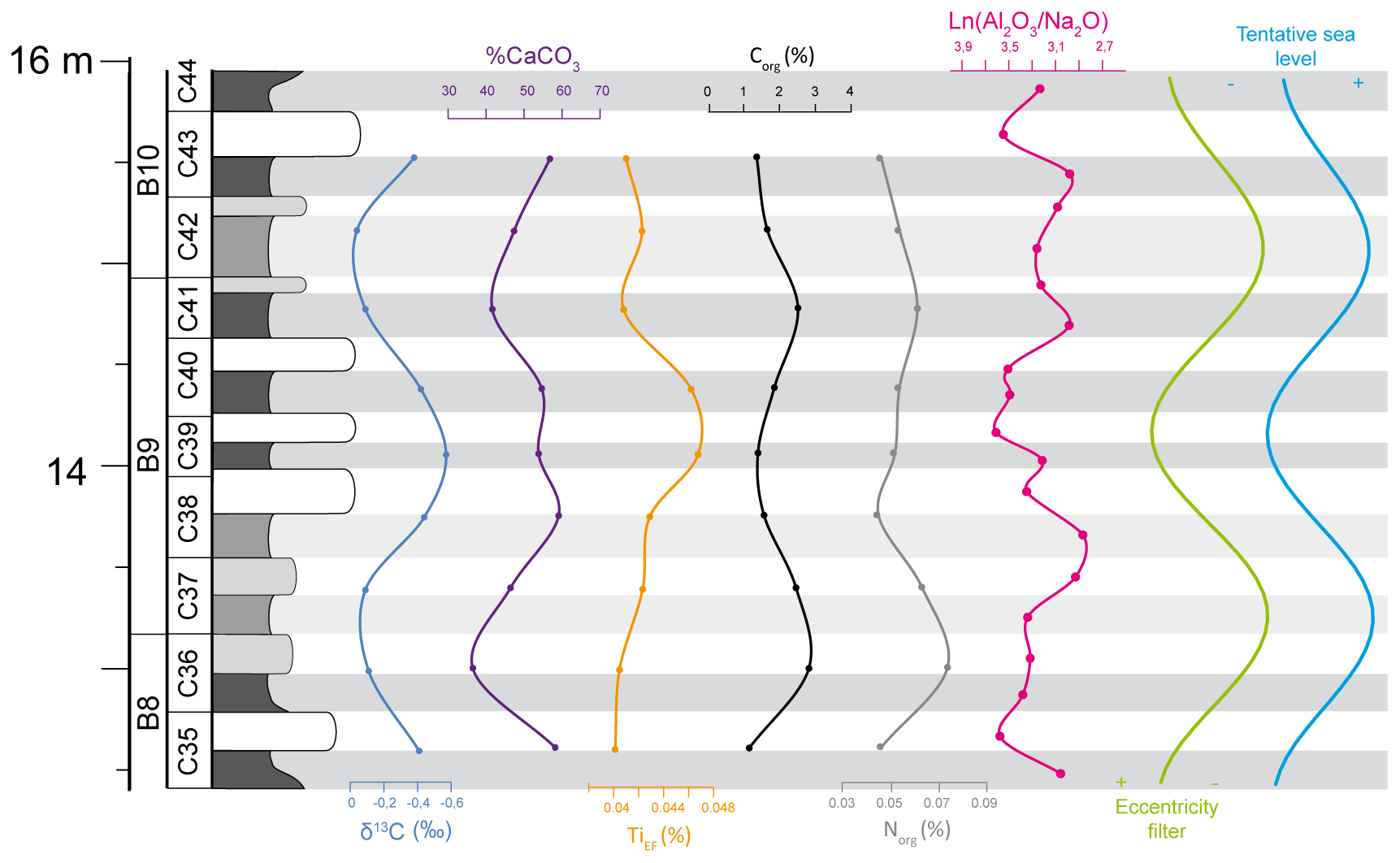
Figure 14 Lithological log of the Santiurde interval studied in detail, showing the average value per couplet of δ¹³C_carb, %CaCO₃, Ti_EF, C_org and N_org. The palaeo-weathering index Ln(Al₂O₃ $/$ Na₂O) of all beds, the short eccentricity colour filter output (Fig. 5), and a tentative sea level curve are also shown.

Minima of Na_EF at high-eccentricity lowstands (Fig. 8) suggest that the climate may have been more humid than during low-eccentricity highstands. The Ln(Al₂O₃ $/$ Na₂O) index is a palaeo-weathering index based on a statistical model of linear compositional and weathering trends (Von Eynatten et al., 2003). This index is especially recommended for rocks with a high percentage of biogenic carbonate (Montero-Serrano et al., 2015), such as those from Santiurde. Ln(Al₂O₃ $/$ Na₂O) values in Santiurde show a gradual trend in line with eccentricity bundles (Fig. 14). Maximum values, which indicate greater chemical weathering in the continent, are recorded at eccentricity maxima. This configuration agrees with the aquifer–eustatic sea level model, in which humid climates result in increased freshwater storage in the continent and lower sea levels, whereas aquifers are emptied in drier periods and sea level rises (Wendler and Wendler, 2016). Jurassic sea level changes deduced from shallower areas from the Iberian basin were also associated with orbitally paced aquifer eustasy (Sequero et al., 2017; Val et al., 2017).

5.3.4 Comparison with orbital forcing during Mesozoic OAEs

Four Lower Jurassic BSIs occur in the BCB and the Asturian basin (Borrego et al., 1996; Rosales et al., 2006). The lower Toarcian BSI correlates with the globally recorded early Toarcian Oceanic Anoxic Event (T-OAE; Jenkyns and Clayton, 1986; Hesselbo et al., 2000; Rosales et al., 2006), which was related to a perturbation in the Earth's climate originated by an abrupt addition of ¹²C into the carbon cycle. Many studies have previously demonstrated the influence of orbital forcing on the T-OAE in western, southern, and northern Tethys areas (Huang and Hesselbo, 2014; Boulila and Hinnov, 2017; Boulila et al., 2019). These studies revealed the general prevalence of 405 kyr eccentricity cycles in Lower Jurassic records, along with a strong expression of both precession and obliquity cycles, although the influence of the latter only increased during the anoxic event. The palaeoenvironmental changes driven by obliquity cycles produced variations in productivity, seabed oxygenation, and/or OM origin during the T-OAE (Suan et al., 2015). The shift in astronomical forcing during the T-OAE has also been linked to the lengthening of the terrestrial productivity season due to increases in global temperatures and humidity (Boulila and Hinnov, 2017; Boulila et al., 2019).

In Santiurde, the influence of eccentricity and precession cycles prevailed during the formation of the Pliensbachian BSI-1, with little or no evidence of obliquity forcing. Interestingly, however, precession cycles also modulated the palaeoenvironmental changes (continental weathering, oceanic productivity and redox conditions) that occurred during other Mesozoic OAEs associated with the release of greenhouse gases, such as the Cretaceous OAE 1a and 1b events (Giogiorni et al., 2015; Benamara et al., 2020). It can therefore be concluded that the Pliensbachian BSI-1 of the BCB shows greater similarities to Cretaceous OAEs than with the Toarcian OAE. However, it should be noted that most of the astrochronological studies of the Early Jurassic, including those focused on orbital forcing on the T-OAE, were previously focused on successions located at latitudes higher than Santiurde (Suan et al., 2015; Martinez and Dera, 2015; Boulila and Hinnov, 2017; Storm et al., 2020). It is possible that, similar to the eccentricity-modulated precessional depositional model, climatic belts determined the response of the sedimentary environment to similar climatic forcings.

6 Conclusions

Lower Pliensbachian organic-rich calcareous rhythmites from the BCB are the expression of periodic environmental variations that occurred in the Milankovitch-cycle band. The cyclostratigraphic analysis of rock colour and magnetic susceptibility data series showed that calcareous couplets represent precession cycles, whereas thicker bundles record short eccentricity cycles; the effect of long eccentricity cycles was also identified.

The integrated sedimentological, mineralogical, and geochemical analysis of a short eccentricity bundle allowed the identification of the environmental factors that governed the formation of the rhythmite, as well as the assessment of diagenetic overprinting. Most of the compositional parameters record primary characteristics related to the formation of the calcareous rhythmites, but inorganic stable isotope records and the distribution of several trace elements may have been somewhat affected by diagenesis during burial. However, the results allowed the definition of an original orbitally modulated depositional model which provides new insight into the formation of lower Pliensbachian organic-rich calcareous rhythmites.

The formation of precessional calcareous couplets was regulated by variations in carbonate productivity and in dilution by terrigenous supply. Thus, organic-rich marls and shales were deposited during precessional configurations, which led to marked annual seasonality (boreal summer at perihelion and winter at aphelion). Increased seasonal rainfall on land and terrigenous input (by rivers or wind) to marine areas boosted organic productivity in surface water. Increased accumulation of organic matter on the seabed eventually caused poorly oxygenated bottom water. Deep-sea deoxygenation and seawater stratification were enhanced due to changes in ocean circulation. Conversely, limy beds were formed when seasonality was minimal (boreal winter at perihelion and summer at aphelion). The consequent decrease in terrigenous inputs favoured a greater production and basinward exportation of carbonate sediment in shallow marine areas. A lower production of OM and increased vertical seawater mixing due to changes in oceanic currents resulted in the oxidation of organic matter in the deepest environments.

In addition, several proxies support the idea that the precessional contrast between the intensity of seasonally controlled environmental factors, such as terrigenous input and oxygenation of bottom water, diminished when the Earth's orbit was circular (minimum eccentricity) and increased when it was more elliptical (maximum eccentricity). The available data further suggest that short-term sea level changes may have occurred in line with short eccentricity cycles (higher sea level at eccentricity minima), probably through orbitally modulated aquifer eustasy.

The comparison with Lower Jurassic successions from other areas suggests that palaeo-latitudinal climatic belts played a significant role in the response of the environment to astronomically forced climate change episodes.

Appendix A

Previous studies demonstrated that the greatest part of the organic matter found in the BCB Pliensbachian black shales had a marine origin, being dominated by amorphous and structured liptinitic organic matter (Suárez-Ruiz and Prado, 1987; Quesada et al., 1997, 2005; Permanyer et al., 2013). The study of saturated biomarkers corroborated a dominant pattern of mature extracts derived from marine algal components. Additionally, SEM analysis carried out in the present study provided evidence of the occurrence of biofilms with sporadic occurrences of vitrinite (Fig. 3e and f).

The average organic C $/$ N ratio of 30.45 obtained in Santiurde (Fig. 7) is significantly higher than that of modern marine organic matter, which usually displays values between 5 and 18 (Meyers, 2006). However, C $/$ N ratios observed in current reservoirs cannot be directly extrapolated to ancient rocks, especially to those deposited under high-productivity conditions (Nijenhuis and Lange, 2000; Meyers et al., 2006; Schneider-Mor et al., 2012). Meyers et al. (2006) observed that organic components from Albian to Santonian black shales from Demerara Rise were mainly marine in origin, but their C $/$ N ratio varied between 20 and 45, which is commonly assigned to terrestrial plants. Those high C $/$ N values were related to a more rapid recycling of N than C during OM decomposition. Modern marine organic matter is commonly degraded via denitrification, principally decomposing nitrogen-rich amino acids and reducing the total organic N of sediments (Altabet et al., 1995; Van Mooy et al., 2002). Thus, high C $/$ N values of some Mediterranean sapropels and Cretaceous black shales have been related to the drawdown of dissolved oxygen in the water column under conditions of high export productivity (Nijenhuis and Lange, 2000; Schneider-Mor et al., 2012). Similar processes might have produced the abovementioned high C $/$ N ratio in Santiurde. In this regard, considering that the C $/$ N ratio of typical marine OM is closer to ∼6, at least ∼23 % of the original N must have been removed from the Santiurde deposits due to denitrification. This percentage is higher than that calculated by experimentation (∼9 %) in recent sediments (Van Mooy et al., 2002) but significantly lower than the 70 % deduced from Cretaceous indurated successions (Schneider-Mor et al., 2012). This suggests that other processes related to OM degradation determine the loss of N due to differential degradation.

The δ¹³C_org signal from Santiurde is also relatively depleted if compared to modern marine OM, being closer to values of terrestrial plants (Schneider-Mor et al., 2012). However, similarly depleted δ¹³C_org values of marine OM have also been found in other indurated successions (Nijenhuis and Lange, 2000; Schneider-Mor et al., 2012). This general depletion of δ¹³C_org compared to average algal tissue is associated with selective decomposition of carbohydrates and proteins enriched in ¹³C_org, which are more easily decomposed, and the fortification of the lipid fraction enriched in ¹²C_org (Jenkyns and Clayton, 1986). A similar fractionation process was invoked in other sections, such as the Cretaceous oil shales from Israel (Schneider-Mor et al., 2012) and the Mediterranean Pliocene sapropels (Nijenhuis and Lange, 2000).

In conclusion, poorly oxygenated background conditions of bottom water triggered denitrification of marine OM in Santiurde, promoting a selective decomposition of nitrogen-rich amino acids and the fraction enriched in ¹³C_org. This process may have been stronger during the deposition of OM-rich shales.