The effect of uncertainties in natural forcing records on simulated temperature during the last millennium

Here we investigate how uncertainties in the solar and volcanic forcing records of the past millennium affect the large-scale temperature response using a two-box impulse response model. We use different published solar forcing records and present a new volcanic forcing ensemble that accounts for random uncertainties in eruption dating and sulfur injection amount. The simulations are compared to proxy reconstructions from PAGES 2k and Northern Hemispheric tree ring data. We find that low solar forcing is most consistent with all the proxy reconstructions, even when accounting for volcanic uncertainty. We also find that the residuals are in line with CMIP6 control variability at centennial timescales. Volcanic forcing uncertainty induces a significant spread in the temperature response, especially at periods of peak forcing. For individual eruptions and superposed epoch analyses, volcanic uncertainty can strongly affect the agreement with proxy reconstructions and partly explain known proxy–model discrepancies.

1 Introduction

To quantify long-term climate variability we rely on simulations from climate models, driven by transient records of past radiative forcing, as well as on climate reconstructions from natural proxy archives. While both sources of information are imperfect in their own ways, they are independent and thus may complement each other and serve for cross-validation. Proxy reconstructions are subject to a wide range of uncertainties and biases, and data availability is sparse in many regions (Wilson et al., 2016a; Anchukaitis et al., 2017; Neukom et al., 2018; Lücke et al., 2019, 2021). Models are very useful for detecting underlying mechanisms and drivers of variability but are only approximations of the real world. Additionally, even a perfect model can only provide data as good as its input parameters: the records of external forcing agents, which are again subject to uncertainties.

Natural climate forcing includes orbital, solar and volcanic forcing. For the last millennium, explosive volcanism is considered to be the main driver of forced surface temperature variability (Crowley and Lowery, 2000; Hegerl et al., 2003; Schurer et al., 2014; Neukom et al., 2019a; Lücke et al., 2019). The influence of solar forcing on large-scale climate variability has been subject to debate, but has probably been minor compared to other forcings (Schurer et al., 2014). Orbital forcing is the only driver that can be precisely calculated for the last few millions of years (Berger, 1978; Berger and Loutre, 1991; Laskar et al., 2004). While it influences seasonal millennial temperature trends (Lücke et al., 2021), it plays only a minor role on shorter timescales.

Volcanic forcing records are most often compiled from sulfate concentrations in ice cores, complemented by documentary evidence to help determine unknown eruption characteristics, including eruption location and precise timing. However, both carry uncertainties, and documentary evidence is not always available, especially for eruptions further back in time (Toohey and Sigl, 2017; Guevara-Murua et al., 2014), and thus various knowledge gaps still exist regarding past volcanic forcing. In some cases, large discrepancies are found between the simulated response to volcanic eruptions and the climate response in proxy reconstructions (e.g. Timmreck et al., 2009; Anchukaitis et al., 2012; Wilson et al., 2016a; Guillet et al., 2017a) but also between the magnitude of ice core sulfate signals and proxy-based climate response estimates (Esper et al., 2017). Studies have shown that the forcing from eruptions can be overestimated if rapid adjustments are not considered (Schmidt et al., 2018) and that the response to eruptions is strongly dependent on the eruption season and latitude (e.g. Marshall et al., 2019, 2020; Toohey et al., 2013, 2019). The latest SAOD reconstruction for the past 2500 years (eVolv2k, Toohey and Sigl, 2017) benefits from improvements in methodologies used to date and synchronise ice core records, resulting in a more accurate estimate of volcanic forcing and resolving some discrepancies in the timing of volcanic events recorded by ice core sulfate records and by temperature-sensitive proxy data (Sigl et al., 2015). Based on data availability and current state of knowledge, the most recent Paleoclimate Project Model Intercomparison Project (PMIP4, Jungclaus et al., 2017) recommends the use of eVolv2k (Toohey and Sigl, 2017) for volcanic forcing in simulations of the past 2000 years, replacing the two previous records (Crowley and Unterman, 2013; Gao et al., 2008) from PMIP3 (Schmidt et al., 2011, 2012). Despite these latest advances, substantial uncertainties remain in the reconstruction of volcanic forcing from ice core records regarding, e.g. timing, magnitude, injection height and latitude of eruptions (Stoffel et al., 2015; Schneider et al., 2017; Stevenson et al., 2017; Marshall et al., 2021). To address this, eVolv2k included an estimated uncertainty range in the volcanic sulfur injections for each eruption for the first time (Toohey and Sigl, 2017), providing information that can be used to explore the impact of uncertainties in volcanic forcing.

Solar forcing is primarily driven by photospheric magnetism, leading to varying numbers of sunspots and faculae concentrations on the solar surface, which modulate the total solar irradiance (TSI). Satellite records start in 1978 and have, in combination with various prior instrumental measurements of TSI, produced a well-constrained understanding of short-term solar activity, which follows a quasi-periodic 11-year cycle (Fröhlich, 2006). Before the start of the instrumental period, sunspot numbers serve as a proxy for TSI. From 1610 CE onwards, records of sunspot numbers from telescope observations are available. However, prior to the telescopic era, the reconstruction of solar variation is based mainly on cosmogenic isotopes deposited in polar ice cores and tree rings, of which solar activity can be estimated by applying a chain of physics-based models. Therefore, long-term changes in radiative forcing remain uncertain, and its exact timeline and especially its amplitude is still controversial (Gray et al., 2010). While most studies suggest a small amplitude on centennial timescales (e.g. Vieira et al., 2011; Steinhilber et al., 2009; Wang et al., 2005; Muscheler et al., 2007), Shapiro et al. (2011) reconstructed the maximum long-term amplitude based on physically possible mechanisms, exceeding other reconstructions by more than 1 W m⁻² during the Spörer Minimum. A number of studies have investigated this high- versus low-amplitude controversy and indicated that high solar forcing is inconsistent with instrumental data (Feulner, 2011; Judge et al., 2012; Lockwood and Ball, 2020) and proxy temperature reconstructions (Ammann et al., 2007; Hind et al., 2012; Schurer et al., 2014). This uncertainty around the long-term solar cycle is reflected by the inclusion of several solar forcing records in PMIP, with three different reconstructions included in PMIP4 (Jungclaus et al., 2017), an update from the previous seven reconstructions of PMIP3 (Schmidt et al., 2011, 2012).

Given the high degree of uncertainty in the volcanic and solar forcing record, it would be desirable to run a variety of comprehensive climate model simulations using different realisations of transient forcing. However, running such experiments over a whole millennium requires large computational resources. Additionally, internal variability tends to disguise the effects of forcing, and therefore a large ensemble of runs would be needed for the differences in the forced signal to emerge for each implementation of forcing. Given the computational expense needed, such experiments are not performed by the scientific community.

A computationally efficient representation of the Earth system is given by simple energy balance models, which simulate the climate system's response to changing radiative forcing (Crowley, 2000; Hegerl et al., 2006; Held et al., 2010; Geoffroy et al., 2013b, a; Millar et al., 2017). Held et al. (2010) introduced an energy balance model with two timescales, in which a fast timescale is associated with the ocean mixed layer, while the slow timescale is associated with the deep-ocean response. Such a model can perform well to simulate the large-scale forced response to greenhouse gas and other forcings on hemispheric and global scale for land and ocean (Haustein et al., 2019).

Here, we use a two-box impulse response model to simulate the response to solar and volcanic forcing, in order to study the consequences of uncertainty in the natural forcing record. We perform experiments using a new ensemble of volcanic forcing, as well as different solar forcing reconstructions as input for the response model. We present the current forcing records, temperature reconstructions and a detailed explanation of the experimental setup in Sect. 2. We compare the response model output to proxy reconstructions of Northern Hemisphere (NH) and global temperature, focusing on the analysis of solar and volcanic forcing uncertainty separately in Sect. 3. The residuals between proxy reconstructions and response model simulations reflect a combination of forcing error, structural error in the response model, tuning error, reconstruction uncertainty and internal variability. We put these residuals into the context of CMIP6 pre-industrial control runs and observed unforced variability. Where the residual is similar in magnitude to internal variability, we conclude that the particular forcing estimate used is consistent with the proxy reconstruction, while the spread of the residuals with varying forcing reflects the importance of forcing error to explain discrepancies. Based on this we estimate the role of forcing uncertainty and evaluate if particular forcings are more realistic than others. We discuss our findings and summarise our conclusions in Sect. 4.

2 Data and methods

2.1 Volcanic forcing

The eVolv2k reconstruction (Toohey and Sigl, 2017) provides a time series of volcanic stratospheric sulfur injection (VSSI) and latitudinally resolved stratospheric aerosol optical depth (SAOD). This reconstruction uses ice core records to estimate the timing and amount of VSSI and the Easy Volcanic Aerosol (EVA) forcing generator (Toohey et al., 2016) to reconstruct the spatiotemporal distribution of SAOD given the estimated eruption latitude, date and VSSI. Estimates of VSSI and SAOD from ice core sulfate measurements have a significant associated uncertainty (Hegerl et al., 2006). The eVolv2k reconstruction provides estimates of the 1-sigma random uncertainty in the VSSI estimates (Toohey and Sigl, 2017). These uncertainties represent uncertainties due to two sources: (1) the uncertainty in the ice sheet (Greenland or Antarctica) mean sulfate flux, based on the variation between the individual ice core records that make up the ice sheet composite, and (2) a representativeness error, corresponding to the error inherent in taking the ice sheet mean as a measure of the full hemispheric sulfate deposition. The latter source of uncertainty is estimated based on the variability in ice sheet average deposition for eruptions of fixed magnitude in aerosol model simulations (Toohey et al., 2013). A total random error is computed by combining the measurement and representativeness error. Average estimated percent uncertainties in eVolv2k are 34 %, with values for eruptions of greater than 10 Tg S ranging from 14 % to 40 %. There is also uncertainty in the timing of eruptions for all but the relatively few ice core sulfate peaks that can be attributed to historically recorded eruptions. For unidentified eruptions, the year listed in the eVolv2k database represents the year in which excess sulfate is first detected in the ice cores, with an estimated uncertainty of ±2 years. This uncertainty includes the overall dating uncertainty of the ice core and uncertainty in the time lag between eruption and first deposition of sulfate flux to the ice sheets. To incorporate uncertainties in VSSI amount and eruption timing into the present work, we constructed an ensemble of VSSI time series from the default eVolv2k data. For each member of the constructed eVolv2k forcing ensemble (eVolv2k-ENS, Fig. S1 in the Supplement), the following steps were taken.

• For each eruption individually, we perturbed the VSSI amount by a normally distributed random variable of mean zero and standard deviation of the reported VSSI uncertainty for that eruption. If the resulting value was negative, we set the value to zero.

• For unidentified eruptions, we perturbed the eruption year by a normally distributed random variable with mean zero and standard deviation of 2, rounded to the nearest integer. Eruption months were also randomised based on a uniform distribution centred on the default January eruption month used in eVolv2k.

This procedure was iterated to produce 1000 different time series of VSSI, each a possible version of past volcanic activity given the estimated values and uncertainties listed in eVolv2k. For each individual eruption, the eVolv2k-ENS members produce a distribution of potential VSSI amount and timing. The original default eVolv2k values are found at the peak of the distribution, representing the estimated most probable value for each individual eruption. The eVolv2k-ENS VSSI time series are then each passed through the EVA v1 forcing generator to create a time series of SAOD. Due to non-linearity in the VSSI to SAOD conversion, the default eVolv2k SAOD is not at the centre of the eVolv2k-ENS SAOD distribution, but it occurs at the peak in the VSSI distribution (Fig. S2). The volcanic forcing ensemble therefore represents an estimate of the range of possible volcanic forcing histories given the VSSI values and random uncertainties reported in the eVolv2k dataset. It does not, however, include all possible sources of uncertainty. For example, it does not include potential systematic biases arising from (i) uncertainty in the scaling relations used to covert ice core sulfate into VSSI or (ii) model uncertainty from EVA, including its lack of sensitivity to the height of the sulfur injection (Aubry et al., 2020). Nor does it include potential uncertainty in the attribution of unidentified eruptions to different latitude bands or any potential misattribution of sulfate signals to historical eruptions.

To convert the global SAOD time series to effective radiative forcing (ERF), we use the average relationship presented for global mean values in Marshall et al. (2020) using exponential scaling (Fig. 1a). The conversion of NH SAOD to NH radiative forcing (Fig. S3a) is more uncertain and therefore, for simplicity, we use the same relationship, in this way treating all of the SAOD ensembles the same. However it should be noted that this presents a substantial source of uncertainty with respect to the impulse response model output, especially for NH results.

Figure 1 Time series of natural forcing records, as anomalies taken over the whole period. (a) Global annual mean of the volcanic forcing ensemble (eVolv2k-ENS) and of eVolv2k. Triangles on top mark the associated eruption years. (b) Solar forcing reconstructions. The three strongest solar minima during the pre-industrial millennium are shaded in grey.

2.2 Solar forcing

Reconstructions of solar irradiance are based on cosmogenic isotope records of ¹⁴C (Roth and Joos, 2013; Usoskin et al., 2016) and ¹⁰Be (Baroni et al., 2015): ¹⁴C is oxidised to CO₂ in the atmosphere and metabolised by trees to form tree rings (e.g. Suess, 1980; Stuiver and Quay, 1980), while ¹⁰Be attaches to atmospheric aerosols, which are removed from the atmosphere in different ways and subsequently deposited to ice sheets (e.g. Beer et al., 1983; Usoskin et al., 2009). They represent independent proxy records (Bard et al., 1997; Steinhilber et al., 2012) and are mostly consistent – especially on long timescales – but deviations during certain periods have been noted due to the different formation rates (Usoskin et al., 2009; Steinhilber et al., 2012).

We include four different reconstructions of solar forcing in our analysis, resulting from either of these isotope records or combined versions, including the PMIP4 records PMOD, SAT10Be and SATC14 (Jungclaus et al., 2017). The latter two are derived from the updated SATIRE-M model (Vieira et al., 2011; Wu, 2017), with SAT10Be using ¹⁰Be isotope records as input, and SATC14 using ¹⁴C isotope records. PMOD uses only ¹⁴C as input (Jungclaus et al., 2017), and represents an update from the older SEA model (Shapiro et al., 2011). PMIP3 includes seven different records (Schmidt et al., 2011, 2012), including, among others, the SBF record (Steinhilber et al., 2009), which was used as the solar forcing record for running HadCM3, and SEA (Shapiro et al., 2011), which represents the maximum-amplitude solar forcing record. Apart from SEA and PMOD, all records represent small long-term solar forcing and share a similar amplitude. Due to the similarities in the low solar forcing records, we restrict our analysis to the PMIP4 records and, for completeness, include SEA, representative of the maximal (although unlikely) physically possible forcing (Fig. 1b). We thus sample two independent isotope records (¹⁰Be and ¹⁴C), combined with two independent reconstruction methods (SATIRE and SEA/PMOD).

The ensemble variance is dominated by the difference in the long-term amplitude (Fig. 1b) and is especially high during the Spörer Minimum (around 1390–1550 CE), the Wolf Minimum (around 1270–1340 CE) and the Maunder Minimum (around 1640–1720 CE) (Usoskin et al., 2007). Short-term changes are less uncertain and are caused by quasi-periodic oscillations ranging between 9 and 14 years (Nandy et al., 2021), mainly as a result of discrepancies between the different isotope records (Usoskin et al., 2009; Steinhilber et al., 2012). The variance is largest during the mid-15th century, coinciding with the large volcanic eruption in 1458 CE. Baroni et al. (2019) hypothesised that large stratospheric volcanic eruptions may deplete the stratospheric ¹⁰Be isotope for around a decade, biassing the isotope records. This could partially explain the large amplitude of solar minima in the SEA record, a record based on ¹⁰Be only, which all coincide with periods of major volcanic activity.

2.3 Impulse response model

2.3.1 Model setup and tuning

The response model accounts for fast and slow temperature changes in response to external forcing (Otto et al., 2015; Haustein et al., 2017; Millar et al., 2017), where fast and slow components are associated with the response of the ocean mixed layer and the deep-ocean response, respectively (Li and Jarvis, 2009). In addition to these two timescale parameters, which need to be determined through model tuning, the equilibrium climate sensitivity (ECS) and the transient climate response (TCR) have to be set. In order to ultimately compare the output with proxy reconstructions, which typically represent Northern Hemisphere (NH) summer (May–June–July–August; MJJA) land surface temperature, we tune the response model separately to global annual temperature and to NH summer land temperature from HadCM3 simulations (Pope et al., 2000; Gordon et al., 2000). We run the response model with TCR = 2.0 and ECS = 3.3 (Tett et al., 2022) and use ICI5 (Crowley and Unterman, 2013) for volcanic forcing and SBF (Steinhilber et al., 2009) for solar forcing, to align with the HadCM3 simulations. Pre-industrial greenhouse gas concentrations (Meinshausen et al., 2017) were converted into radiative forcing (Etminan et al., 2016) and merged with historical output from FAIR v1.3 (Smith et al., 2018). Aerosol forcing from the Community Emissions Data System (CEDS, Hoesly et al., 2018) is included from 1820 CE onwards. We tune the response model by minimising the residuals between the response model output and the all-forcing HadCM3 ensemble mean over the period 1400 to 1850 CE. We use the HadCM3 all-forcing simulations as the target for tuning to ensure an optimal choice of the fast and the slow response time. We test the tuned response model by comparing its forced response separately to the all-forcing HadCM3 ensemble mean as well as to individual forcings (Figs. S4 and S5). Note that the response to solar forcing in the HadCM3 solar-only simulation is largely masked by residual internal variability in the ensemble mean, which decreases the correlation between HadCM3 and the response model. For greenhouse gas (GHG) and volcanic forcing we confirm that the best fit corresponds well with the associated HadCM3 ensemble mean.

2.3.2 Forcing uncertainty ensemble

After determining the free model parameters, we run the response model with our forcing uncertainty ensemble as input. However, to ensure an optimal comparison between response model and proxy reconstructions, we first change the climate sensitivity to a more generic setup. A large range of climate sensitivity is found across the CMIP6 models (Fig. S6), reflecting the large uncertainty associated with this parameter (Sherwood et al., 2020). We therefore run the response model with the median climate sensitivity across CMIP6 (ECS = 3.3, TCR = 2.0) for the main analysis and conduct additional sensitivity studies with the lower and the upper range of climate sensitivity of CMIP6 models (shown in the Supplement). The lowest climate sensitivity is associated with INM-CM4-8 (ECS = 1.84, TCR = 1.32), and the highest climate sensitivity is associated with E3SM-1-0 (ECS = 5.38, TCR = 2.99). This way we can estimate a lower and an upper limit of the temperature response to differences in the natural forcing record.

In order to run the impulse response model with eVolv2k-ENS, we convert the forcing time series from SAOD to ERF. For producing global annual data, we use the globally averaged time series of SAOD, while for NH summer, we restrict our data to NH SAOD only. For global data, yearly averages are created by using the average from April to March of the following year, following Neukom et al. (2019a). For NH summer data, we use a similar strategy; e.g. for a given year we average September of the preceding year to August of the current year. This way, we ensure that a volcanic eruption after the growing season has finished is not taken into account for a given year. The resulting time series are converted into ERF using the non-linear scaling (Marshall et al., 2020).

The 1000 time series of volcanic radiative forcing obtained by eVolv2k-ENS are joined with the four solar forcing time series, and thus the response model is run 4000 times for each global annual and NH summer land temperature. Greenhouse gas and aerosol forcing were kept from the previous setup. Additionally, we run the response model with the PMIP4 reference forcing eVolv2k.

A summary of the complete process, from model tuning to running the forcing uncertainty ensemble, is given in Fig. S7.

2.4 Evaluation of the forced response

2.4.1 Residual variability of proxy reconstructions

To evaluate the consistency between the output of the impulse response model x, which constitutes the temperature response to radiative forcing, and the proxy reconstructions y, which record the temperature variability due to forcing and internal variability, we calculate the residuals using the root-mean-square error (RMSE). We calculate the RMSE over centred running windows t with length N using

$$\begin{array}{}\text{(1)}& \begin{array}{rl}& {\mathrm{RMSE}}_t=\sqrt{{\displaystyle \frac{\mathrm{1}}{N}}\sum _{i=-N/\mathrm{2}}^{N/\mathrm{2}}{\left(\left(x_{i+t}-{\widehat{x}}_t\right)-\left(y_{i+t}-{\widehat{y}}_t\right)\right)}^{\mathrm{2}}},\\ & t={\displaystyle \frac{N}{\mathrm{2}}},{\displaystyle \frac{N}{\mathrm{2}}}+\mathrm{1},{\displaystyle \frac{N}{\mathrm{2}}}+\mathrm{2},\mathrm{\dots }\end{array}\end{array}$$

The mean over the window t is denoted by ${\widehat{x}}_t$ for the response model and ${\widehat{y}}_t$ for the proxy data. We choose a length N=20 years to analyse the temperature response to volcanic forcing and a length N=200 years to analyse the response to solar forcing. The former encompasses the recovery time even after a large volcanic eruption such as Tambora generously (A. P. Schurer et al., 2013; Otto-Bliesner et al., 2016; Raible et al., 2016). The latter encompasses a full solar cycle, which has an amplitude of around 200 years (Fig. 1b). The residual represents differences between model output and proxies due to internal variability present in the proxy reconstructions but also includes the discrepancy between radiative forcing in the proxies and the model, proxy reconstruction error, and model simulation error.

We can roughly estimate the influence of all of these factors by

• varying the radiative forcing in the response model using an ensemble of different realisations of forcing to estimate forcing discrepancy,

• comparing the residuals to control runs from climate models and to estimates of unforced variability in observational data to estimate internal variability,

• using an ensemble of different proxy reconstructions to estimate reconstruction error,

• comparing the response model simulations to coupled climate model simulations to estimate simulation error.

2.4.2 Proxy reconstructions

We use four tree ring reconstructions of Northern Hemispheric (NH) summer temperature (N-TREND16: Wilson et al., 2016a; N-TREND17: Anchukaitis et al., 2017; GCS17: Guillet et al., 2017a; SSB15: Schneider et al., 2015a) and the multi-proxy reconstruction PAGES 2k (Neukom et al., 2019a) for global annual temperature. The N-TREND reconstructions are both compiled from the Northern Hemisphere tree ring network development dataset (Wilson et al., 2016a; Anchukaitis et al., 2017) but using different reconstruction methods. N-TREND16 is a hemispheric land surface temperature reconstruction based on iterative nesting plus scaling to instrumental data. N-TREND17 is a climate field reconstruction using point-by-point regression (Cook et al., 1999). N-TREND includes measurements of tree ring width (RW), maximum latewood density (MXD) and blue intensity (BI) and aims to reconstruct midlatitudinal (40–75^∘ N) MJJA temperature over land. SSB15 uses weighted composites based on moving correlations with local temperature and scaling to reconstruct extratropical (30–90^∘ N) June to August (JJA) temperature. They include solely MXD tree ring chronologies, which are considered to be more sensitive to high-frequency variability (Franke et al., 2013; Esper et al., 2015; Lücke et al., 2019). GCS17 uses tree ring data (RW and MXD) to reconstruct extratropical (40–90^∘ N) JJA temperature over land with a bootstrap linear model using principal component analysis. The four reconstructions share several chronologies; however, all of them use different methodologies for reconstruction.

PAGES 2k uses a large multi-proxy dataset (PAGES2k Consortium, 2017) and combines seven different reconstruction methods (Neukom et al., 2014; Mann et al., 2008; Luterbacher et al., 2002; Shi et al., 2017; Hanhijärvi et al., 2013; Barboza et al., 2014; Hakim et al., 2016) to obtain global mean surface temperature (GMST) of the last 2 millennia between April and March. For each method Neukom et al. (2019a) obtained an ensemble of 1000 reconstructions using various statistical approaches to estimate the reconstruction uncertainty such as bootstrapping or red noise perturbations. For computational reasons we subsample 50 random ensemble members of each method, which we find gives a reasonable estimate of the ensemble spread (compare Fig. S8).

2.4.3 Time series filtering

We apply a second-order Butterworth filter (Mann, 2004, 2008; Neukom et al., 2019a) on all temperature time series, which we use in two ways: to isolate the response to a specific forcing and to suppress the spectral biases and frequency insensitivity of the proxy data. To isolate the response to long-term changes in solar variability we use a bandpass filter between 50 and 300 years. PAGES 2k and N-TREND are both sensitive to temperature variability on this frequency band (Neukom et al., 2019a; Lücke et al., 2019). For the volcanic response we focus on annual to multi-decadal frequencies. However, PAGES 2k was shown to be relatively insensitive to high-frequency variability due to the large inclusion of low frequency records (Neukom et al., 2019a), and thus we set the high-frequency threshold at 15 years for global analyses. Tree ring reconstructions perform well at high frequencies but are subject to autoregressive biases which affect their high-frequency variability (Lücke et al., 2019). We therefore set the high-frequency threshold at 5 years. The low-frequency threshold remains set at 300 years.

2.4.4 Variability of CMIP6 control runs

We use temperature data from 58 pre-industrial control runs (Eyring et al., 2016, Table S1 in the Supplement) to estimate unforced temperature variability on centennial timescales and on multi-decadal timescales. Temperature was averaged over both midlatitudinal land summer (MJJA) and the global annual mean. The time series were bandpass filtered, and the RMSE was calculated from non-overlapping chunks of N=20 and N=200 years. For N=20 years all individual models are consistent within the lower and upper quartile of the population of all simulations, showing that most of the models roughly agree on the extent of decadal variability (Fig. S9a and c). For N=200 years there is less agreement between the individual models, with some models displaying higher variability than others (Fig. S9b and d). These models are also associated with higher 100-year running GMST trends (Parsons et al., 2020), and we therefore refer to them as high-variability types.

2.4.5 Residual variability of observations

We use the infilled HadCRUT5 dataset (Morice et al., 2021), a gridded dataset of global historical surface temperature anomalies from January 1850 to December 2020. The infilled dataset has increased coverage and includes 200 realisations sampling the distribution of various errors and uncertainties. To obtain an estimate of unforced variability, we conduct a total least-squares (TLS) regression, using the historical CMIP6 multi-model mean as the fingerprint of forcing (Allen and Stott, 2003; Schurer et al., 2014). The residuals give an estimate of the unforced variability (Schurer et al., 2015; Friedman et al., 2020) and can be compared to the residuals of proxy and model simulations. This procedure was repeated for each of the HadCRUT5 ensemble members and for both global annual and NH summer temperatures.

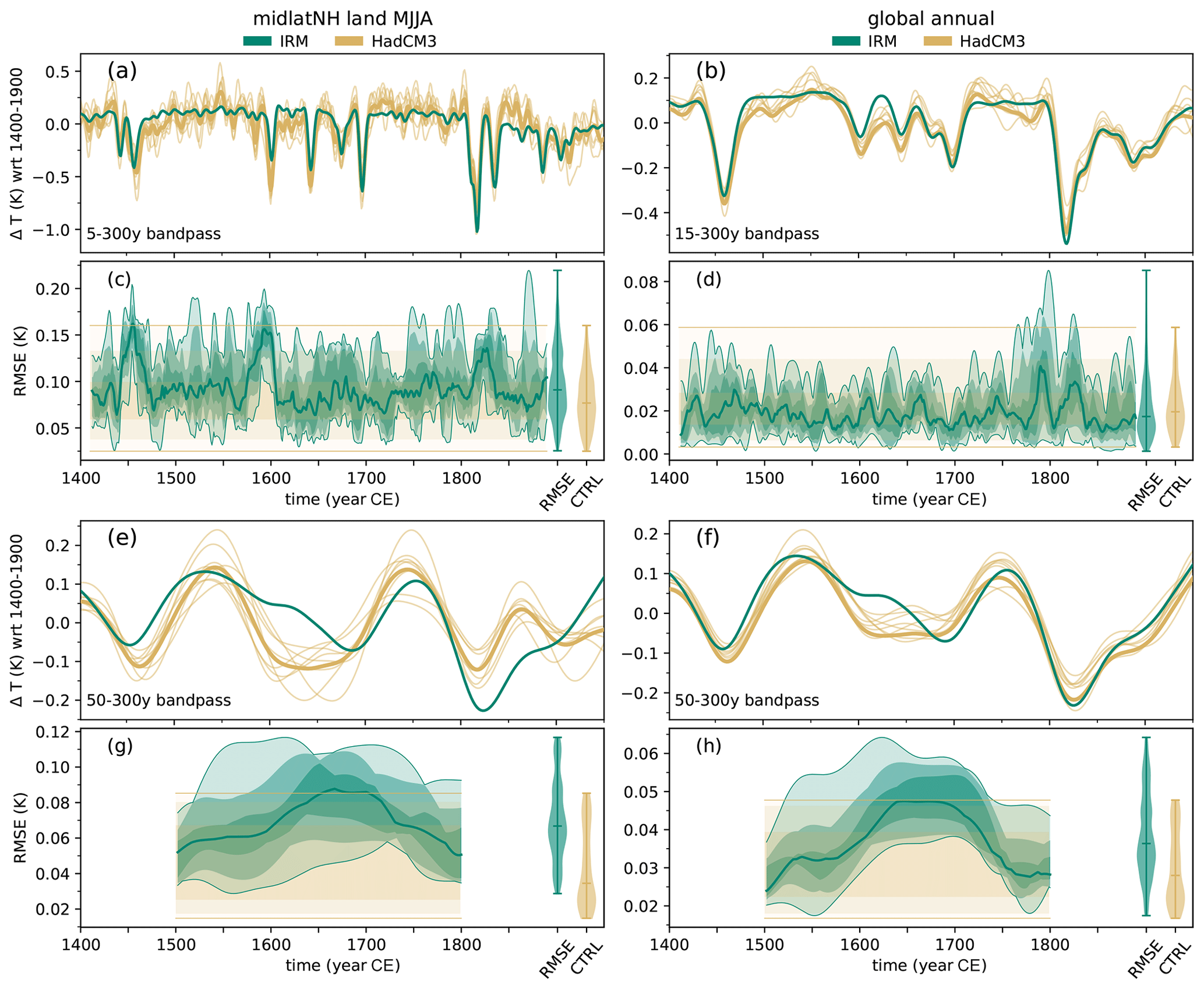
Figure 2 Evaluating the performance of the response model, tuned to HadCM3 and using similar forcing, against simulations from HadCM3. (a, c, e, g) Mid-latitudinal NH land MJJA temperature. (b, d, f, h) Global annual temperature anomalies. (a, b) Bandpass-filtered time series of the past 600 years. The thick orange line represents the HadCM3 ensemble mean, and thin lines show the ensemble members. (c, d) RMSE between impulse response model (IRM) and HadCM3 versus HadCM3 control (CTRL) variability calculated over 20-year running windows. Thick lines represents the median, and shading represents the 75th, 90th and 100th percentile. The violin plots show the distribution of all slices. (e–h) As above but filtered using a 50–300-year bandpass and residual variability calculated over 200-year windows.

3 Results

3.1 Model performance

We assess the model performance by comparing the residuals between the response model, tuned to HadCM3 and using HadCM3 forcings, and transient HadCM3 simulations to the standard deviation of HadCM3 control runs over 20- and 200-year sliding windows (Fig. 2). For a perfect response model, which accurately reproduces the climate response to forcing in HadCM3, the residuals would represent the internal variability simulated by HadCM3 and thus match the spread of control variability. However, given that the response model is a simplistic simulation of large-scale climate and does not account for hemispheric transport, seasonal processes or non-linear mechanisms, we expect the residuals to also include model error and thus to exceed the control variability. Remaining internal variability in the HadCM3 ensemble mean due to the relatively small ensemble size could additionally increase the residuals.

At 20-year timescales the residuals mostly agree with the spread of control variability, especially for global simulations. However, in the NH, residuals are very large during the mid-15th century as well as around 1800, which are both periods of high volcanic forcing. The larger residuals around 1800 are also present in the global simulation. Both periods are subject to very large volcanic forcing, and thus it is likely that the response model may be too simplistic to accurately model the associated climate processes as simulated by HadCM3. We find a larger discrepancy for both global and NH simulations at the 200-year timescale, although the 90th percentile is within the range of control variability at most times. The residual clearly exceeds the control variability during the 17th century, which could be explained by a possible non-linearity in the solar and volcanic forcing during that period (Schurer et al., 2014). As observed at the 20-year timescales, residuals are smaller for global simulations, indicating that model error is larger in the NH. This finding is unsurprising, given that regional and seasonal climate processes play a larger role for NH summer temperature as opposed to global annual temperature.

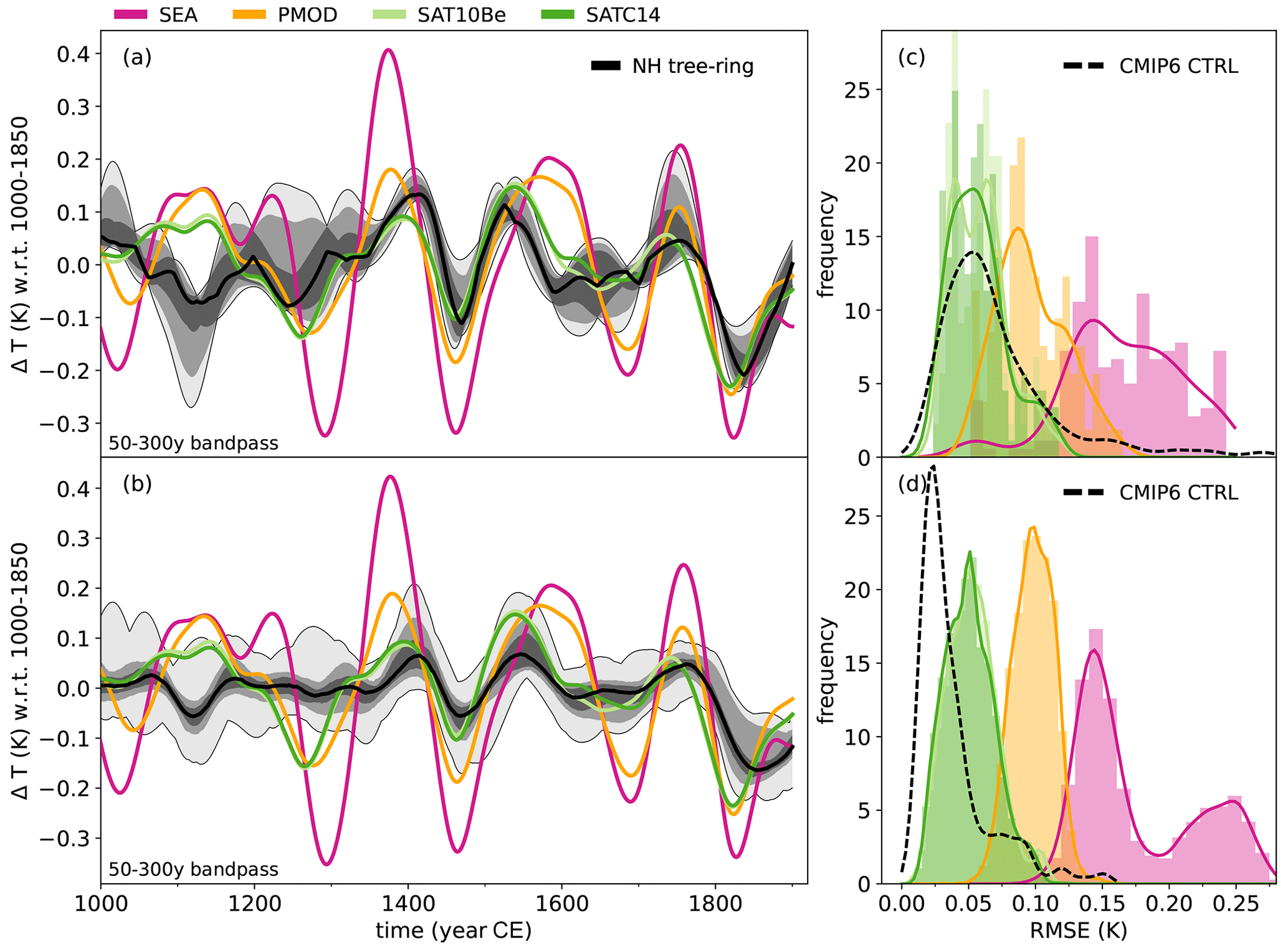
Figure 3 (a, b) Temperature anomaly of proxy reconstructions and response model ensemble for the different solar forcing records for (a) NH summer land and (b) global mean, filtered by a 50–300-year bandpass. The shading indicates volcanic forcing uncertainty for the response model and reconstruction uncertainty for the proxy data (shading levels at 75th, 90th, and 100th percentile; the thick line shows the median; thin lines show the range). (c, d) Distribution of residuals between response model and proxy reconstructions, calculated over 200-year sliding windows over the period 1300 (dotted line in a and b) to 1900 CE, for (c) NH summer land and (d) global annual temperature for different solar forcing estimates (colours). The dashed line indicates the variability of CMIP6 control runs.

3.2 Solar forcing uncertainty

We compare the proxy reconstructions with response model simulations including the different solar forcing reconstructions. On centennial timescales the difference between simulations including SAT10Be and SATC14 is almost negligible, and both follow the proxy reconstructions closely after around 1300 CE (Fig. 3a and b). In contrast, the temperature response to PMOD and SEA forcing show very large variability, with particularly strong anomalies during the Wolf (around 1300 CE) and the Spörer (15th century) minima. Since the availability of proxy records decreases quickly before 1300 CE, and therefore reconstructions are much more uncertain (Wilson et al., 2016a; Neukom et al., 2019a), we use the period from 1300 to 1900 to calculate residuals between proxy reconstructions and response model simulations and compare to estimated observed and modelled internal variability. The residuals between the proxy reconstructions and the full response model ensemble show that even when accounting for volcanic and proxy reconstruction uncertainty the SATIRE forcings consistently generate the lowest residuals, and SEA consistently generates the highest (Fig. 3c and d), with very little overlap between them. For the Northern Hemisphere, the former shares a very similar distribution with the root-mean-square deviation of the CMIP6 control variability, although the distribution shows two peaks, generated by different proxy reconstructions. Given that the model error ranges around 0.03 K for NH summer simulations and 0.01 K for global annual simulations (Fig. 2), we expect the response model to produce slightly higher residuals than the control variability. This suggests that SATIRE forcing is consistent with the reconstructions compared to the distribution of control variability. In contrast, both PMOD and SATIRE are inconsistent with the majority of CMIP6 control runs.

At the global scale, the CMIP6 control runs show a significantly lower variability than the residuals from all solar forcings. This is roughly consistent with the difference between HadCM3 and the response model run with HadCM3 forcing (Fig. 2) and thus could be caused by model error or could indicate that global annual variability is slightly underestimated by CMIP6 models. PMOD is only consistent with the upper tail of the distribution, caused by the high-variability-type models, and residuals from SEA are pretty much inconsistent with CMIP6 control variability.

It is worth noting that the relative magnitude of residuals associated with the different solar forcings is independent of the temperature target and the reconstruction (Figs. S10 and S11). In addition, it is also independent of response model parameters such as climate sensitivity. While for the low climate sensitivity the differences between the temperature response to SATIRE, PMOD and SEA forcing decrease, SEA still produces consistently larger residuals than SATIRE forcing (Fig. S12). For the high climate sensitivity the differences increase (Fig. S13), but the order remains unchanged: SATIRE produces the smallest residuals, followed by PMOD and finally SEA forcing.

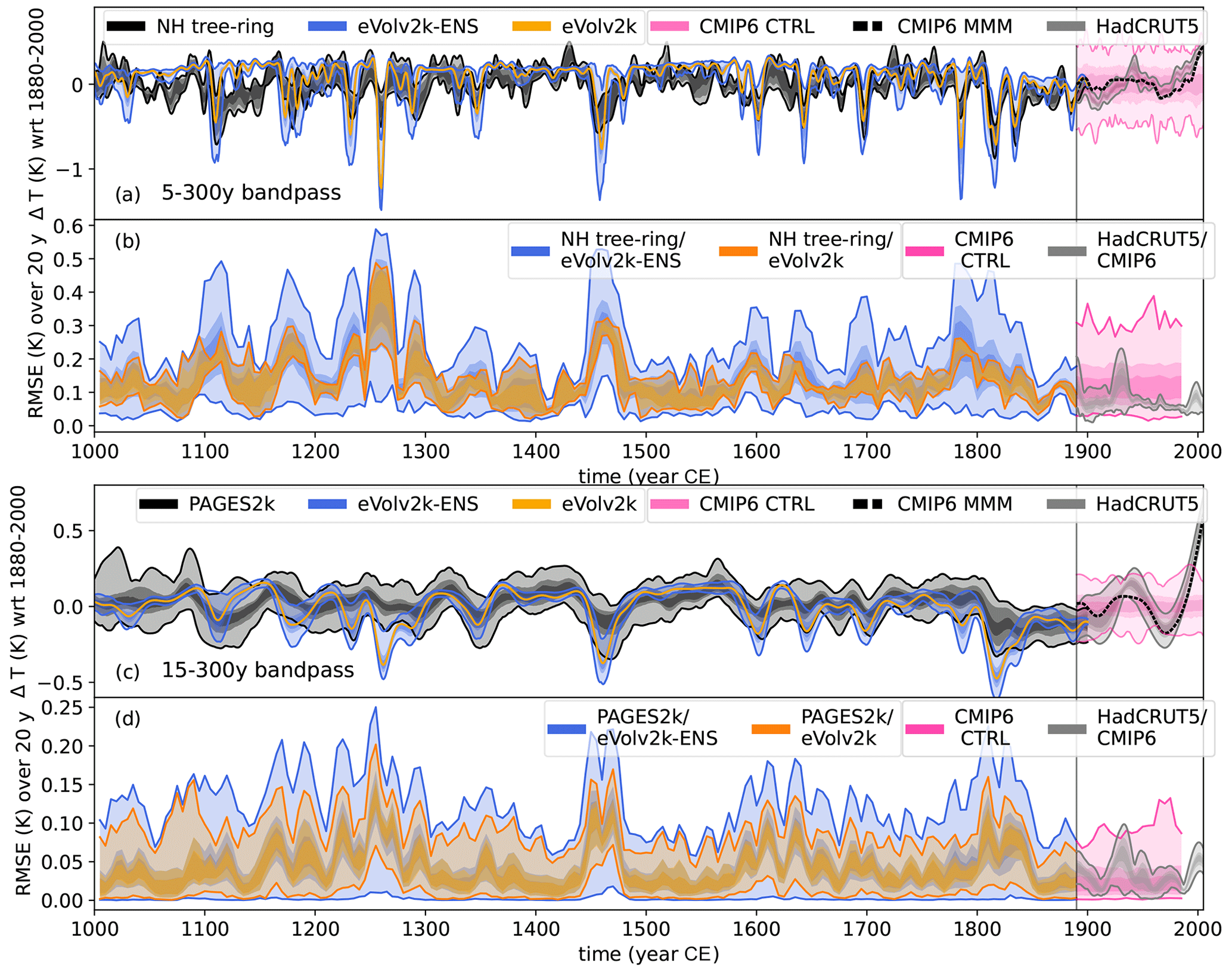
Figure 4 (a) Temperature anomaly from tree ring reconstructions and response model simulations for NH land summer over the pre-industrial last millennium (up to 1885 CE), filtered by a 5 to 300 years bandpass. Observations, CMIP6 historical multi-model mean (MMM) and CMIP6 control runs are presented from 1885 onwards. Note that the CMIP6 control runs are shown for reference only and are not associated with this particular time period. (b) Residuals between tree ring reconstructions and response model simulations over 20-year running windows. From 1890 onwards residuals between HadCRUT5 and the CMIP6 multi-model mean are shown and compared to CMIP6 control variability. Panels (c, d) are the same as (a, b) but for global annual data and compared to PAGES 2k using a 15- to 300-year filter. The shading in all panels indicates the 75th, 90th, and 100th percentile; thin lines show the range; and thick lines show the median (where applicable).

3.3 Volcanic forcing uncertainty

To quantify the effect of volcanic forcing uncertainty, we fix the solar forcing to SATC14, the default PMIP4 forcing (Jungclaus et al., 2017). The volcanic ensemble generates a large variety of amplitudes in response to individual eruptions. At times, the spread between the ensemble members exceeds 1 K in the NH, indicating that large uncertainty of the volcanic forcing record progresses into the temperature response (Fig. 4a). The largest spread is found during the 1450s CE, and after the eruption of Laki (1783 CE). Accordingly, the magnitude of the residuals between response model simulations and proxy reconstructions also varies significantly throughout the millennium (Fig. 4b). In the NH, the 75th percentile of the residuals obtained from eVolv2k-ENS agrees with the spread of residuals obtained from eVolv2k, which represent the proxy reconstruction uncertainty, at most times. The proxy reconstruction uncertainty tends to be larger during years of low volcanic activity, and decreases around the eruptions, except for the eruption of Samalas in 1257 CE. The residuals of eVolv2k-ENS are largest and show the largest spread during periods of high volcanic activity. The residuals peak around the eruption of Samalas for both eVolv2k and eVolv2k-ENS, which also features the largest spread of results. This reflects the large uncertainty around this eruption with regard to both forcing and reconstruction. The mismatch between the model response to the eruption of Samalas and the response shown by proxy reconstructions is a well-known discrepancy. It reflects a mismatch between the signals in ice cores, the source data of the volcanic forcing in model simulations, and tree rings, the source data of the proxy reconstructions (Guillet et al., 2017a; Timmreck et al., 2009). Additionally, the response model and the proxy reconstructions match better going forwards in time, with a particularly poor agreement prior to ca. 1300 CE. This reflects the decreasing data availability and quality as we go back in time. Prior to 1300 CE only few high resolution MXD records are available, which reduces the confidence in the proxy reconstructions for the first 3 centuries (Wilson et al., 2016a) and hence in the proxy response to the eruption of Samalas. Nevertheless, given the large ensemble spread between residuals from the eVolv2k-ENS members (around 0.2 K) around this eruption, volcanic forcing uncertainty could additionally explain a part of this discrepancy. A similar observation holds for the mid-1450s CE eruptions (Esper et al., 2017; Sigl et al., 2015); however, in this case the spread of reconstructions is smaller.

While volcanic forcing uncertainty provides a possible contribution to the discrepancy of these specific eruptions, it is unlikely that it can be fully explained by it – at least not with such a simple model. Proxy biases, reconstruction uncertainty and model errors may provide further explanations. Apart from Samalas and the mid-1450s eruptions, the lower range of residuals is well in line with the observed unforced variability. Thus, for most eruptions we can find an ensemble member that is in line with the uncertainty range of observed internal variability and control variability. It is likely that the lowest range overfits the data to some extent; however, it is well in line with observed unforced variability (Fig. 5a). For most of the instrumental period – except the 1920s – the 20-year variability of control runs exceeds the estimates of observed unforced variability. Based on these findings, we conclude that for many eruptions, the temperature differences resulting from volcanic forcing uncertainty are in line with the magnitude of internal variability on decadal timescale. This indicates that differences in the response to volcanic eruptions due to uncertainty in the eruption parameters may not emerge from the background of internal variability. This is particularly important for comparing model simulations to proxy reconstructions. For eruptions that exceed the control variability, it is likely that the proxy temperature reconstructions can constrain the volcanic forcing by identifying forcing ensemble members that produce temperature anomalies incompatible with the reconstructions. This includes, for example, the 1345 CE eruption, the Samalas eruption, the unknown mid-15th century eruption, the tropical eruptions in the 17th century (1600, 1640, 1695), the Laki eruption (1783) and the 19th century eruptions (1809 and Tambora 1815). However, residuals from most of eVolv2k-ENS and residuals from eVolv2k fully agree with the range of control variability after 1300 CE (Fig. 5a).

Figure 5 Distribution of residuals between proxy reconstructions and impulse response model simulation from 1300 to 1900, compared to the distribution of CMIP6 control variability and estimated unforced variability in HadCRUT5. Panel (a) shows NH land summer temperature, and panel (b) shows the global annual temperature. The proxy/eVolv2k-ENS lower range represents the lower range of the residuals (thick blue line) shown in Fig. 4b and d.

The ensemble spread for global temperature is less variable, and the biggest spread just about exceeds 0.3 K (Fig. 4c). This is partly caused by the smaller variability of global annual temperature in contrast to NH land summer temperature, and thus it could be an effect of the tuning. It could also reflect a possibility that random errors average out in the global reconstruction. However, note that high-frequency variability is strongly suppressed due to the bandpass filter that we applied to global annual temperature (compare Fig. S14).

At global scale, the 90th percentile of the uncertainty ensemble agrees at all times with the range of eVolv2k residuals. This implies that after removing the higher frequencies with the 15- to 300-year bandpass filter, spread due to volcanic forcing uncertainty is small compared to the proxy uncertainty range. We therefore concentrate on the analysis of the residuals from NH reconstructions and simulations. However, we note that the lower range of the eVolv2k-ENS spread perfectly matches the lower range of the control variability at all times for the global residuals and exceeds the upper range only during periods of very large volcanic forcing. Thus, eVolv2k lies well within the range of control variability, and at times of low volcanic forcing the residuals of PAGES 2k/eVolv2k, CMIP6 control runs and the residuals of HadCRUT5/CMIP6 match almost perfectly. However, it is likely that the lowest range is an overfit of the data (see Fig. 5b) due to due to a large number of degrees of freedom.

Our results suggest that internal variability and proxy reconstruction uncertainty may at times disguise the effects of volcanic forcing uncertainty, which range in the same order of magnitude. However, overall, they confirm the large-scale quality of proxy reconstructions, where the distribution of residuals between eVolv2k and proxy reconstructions overlaps well with the distribution of control variability and observed unforced variability (Fig. 5).

Note that due to the way eVolv2k-ENS was compiled, it does not represent systematic uncertainty, but it instead randomly combines the uncertainties associated with individual eruptions. Thus, the distribution of the residuals over the whole millennium do not differ very much between the different ensemble members (Fig. 5). Compared to eVolv2k, the main difference can be found at the upper tail of the distribution, which, for most ensemble members, is shifted towards larger residuals. In Fig. 4b and d, the lower range represents the minimum residual that can be generated by one ensemble member over 20 years. Due to the limited ensemble size of 1000 ensemble members, randomly combining 105 eruptions, the lower range does not represent one individual ensemble member but a combination of them over the whole millennium for each 20-year slice. While this may strongly overfit the data due to the large number of degrees of freedom, it can give information about the very lowest boundary of residuals that can be achieved by tweaking the volcanic response. Remarkably, the lower range of NH residuals fits the estimate of observed variability relatively well (Fig. 5a), although the left tail of the distribution indicates that a significant number of residuals approach zero. This is not consistent with any other data source, and it thus clearly indicates overfitting. For global data, the same observation can be made, and the distribution of the lower range is considerably smaller than control and estimated observed variability. However, the large discrepancy between the distribution of eVolv2k-ENS and the distribution of the lower range of residuals indicates that choice of the volcanic forcing record can influence the variability of last millennium temperature significantly, especially at (but not limited to) higher frequencies.

As a sensitivity study, we repeat our analysis with the highest and the lowest climate sensitivity presented by a CMIP6 model. We find that for very high climate sensitivity, the differences between the ensemble members are much elevated (Fig. S15), making the residuals overall less consistent with control variability (Fig. S16a and b). This concerns both residuals obtained from eVolv2k and eVolv2k-ENS, although the best fit considerately overlaps with control and observed variability. In contrast, very low climate sensitivity suppresses the response to forcing and thus decreases the spread of eVolv2k-ENS (Fig. S17), and the distribution of residuals is shifted towards zero (Fig. S16c and d). Consequentially, if climate sensitivity was very low, the effects of volcanic forcing uncertainty may be to a very large extent disguised by internal variability.

The exact effect of timing and magnitude uncertainty on the temperature response to individual eruptions can be quantified by focusing on the 11 eruptions with the largest eruption magnitudes (Fig. 6a–k). Due to the better high-frequency sensitivity of NH reconstructions, we limit our analysis to NH temperature. Furthermore, we consider only eruptions past 1300 CE due to the increased quality of proxy reconstructions (Wilson et al., 2016a). We compare the eVolv2k-ENS ensemble spread to the proxy reconstructions and find the forcing ensemble members that minimise the residuals between response model and each proxy reconstruction. For most eruptions we find at least one ensemble member that matches the proxy reconstruction very closely in the immediate aftermath of an eruption, in particular for the eruptions of 1345, 1640, 1695 and 1783, as well as all 19th century eruptions. This has a significant effect on the superposed epoch analysis that combines these eruptions (Fig. 6l) and brings the simulated volcanic response in line with the proxy reconstructions. Eruptions that still show a significant discrepancy include those of 1453, 1458 and 1600.

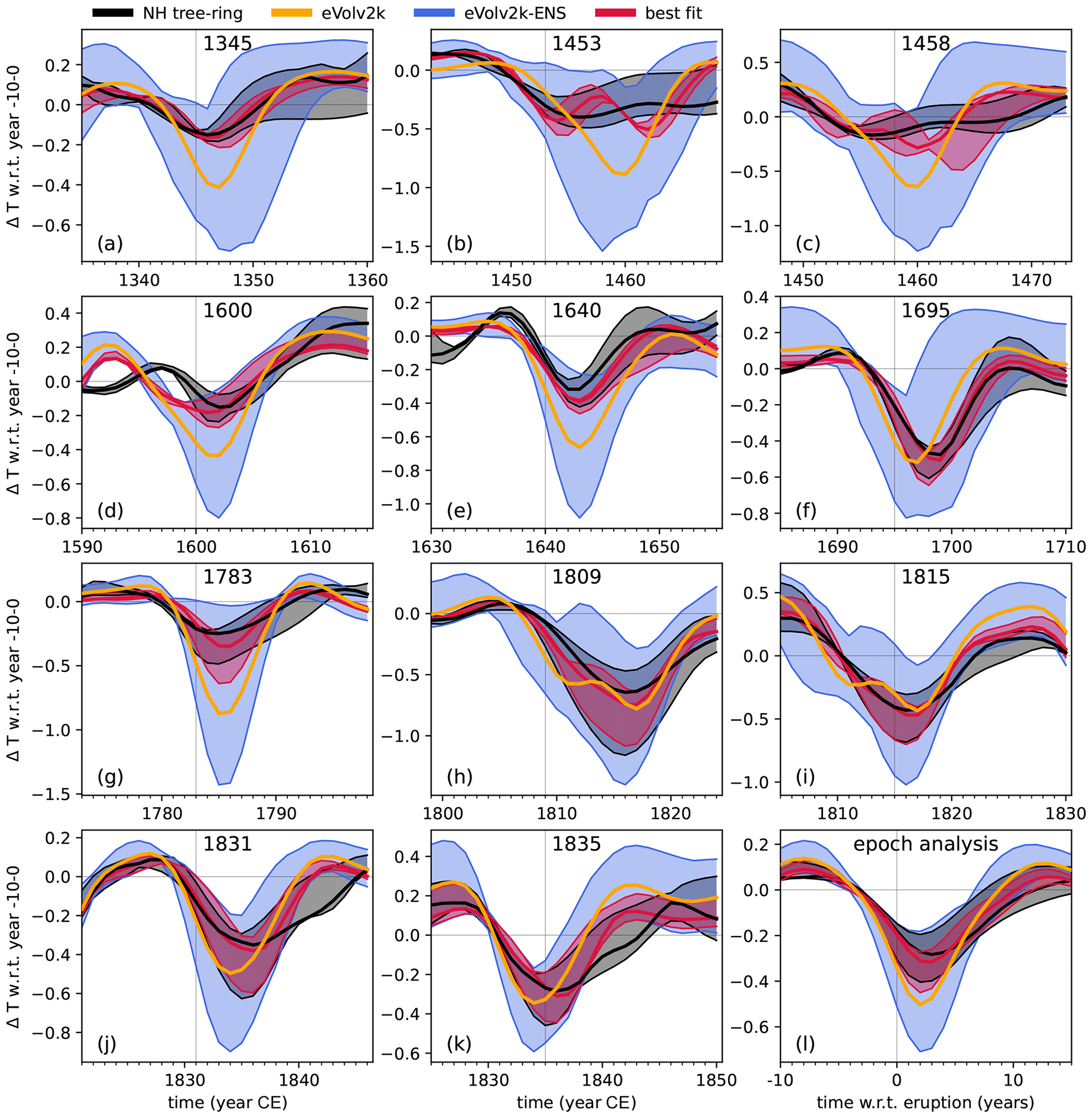
Figure 6 (a–k) Temperature response to the 11 biggest eruptions post 1300 CE, filtered by a 5- to 300-years bandpass. Title indicates the eruption year in eVolv2k. Anomalies are taken with respect to 10 years prior to the eruption in eVolv2k up to the eruption year. (l) Epoch analysis over all eruptions shown in panels (a)–(k). In all panels the shading indicates the range, and the thick line shows the median (where applicable). The red line and shading indicates the best fitting ensemble members, relative to the four different reconstructions.

Comparing the eruption parameters of eVolv2k-ENS best fit and eVolv2k, we find that for most eruptions the sulfate injection magnitude favoured by the proxy reconstructions is significantly reduced (Table S2 and Fig. S18). Only for the 1453 eruption do all four reconstructions suggest a larger sulfate injection magnitude than eVolv2k, while for the 1835 eruption three reconstructions agree on a slightly larger one. For all other eruptions considered, the majority of proxy reconstructions suggest smaller eruption amplitudes, with a reconstruction average ranging from 32 % for Laki (1783) to 88 % for Tambora (1815). From the four reconstructions considered, GCS17 stands out regarding the magnitude, suggesting a higher magnitude for about half the eruptions considered (1453, 1695, 1809, 1815 and 1835).

For undated eruptions, eVolv2k-ENS accounts not just for the uncertainty of sulfate injection, but also for uncertainty in eruption month and year. Out of the 11 eruptions shown in Fig. 6, this concerns the eruptions of 1345, 1453, 1458, 1694 and 1809. While the eruption year plays a role regarding the spread of the temperature response, the eruption month does not seem to account for much variance (Fig. S19). It is likely that this is caused by the simple nature of our temperature response model, which does not take seasonal processes into account, and thus we cannot draw any significant conclusions regarding the role of the eruption season. The relative eruption year varies greatly between the different undated eruptions, as well as the different reconstructions, with no visible trend (Fig. S20). We find that only for the 1695 eruption do all reconstructions agree on a slightly later eruption date, ranging between +1 and +3 years. For the other eruptions results range between −2 and +3 years.

The wide range of volcanic forcing uncertainty found in the temperature response to the 11 individual eruptions leads to a similarly large range in the epoch analysis combining these eruptions (Fig. 6l). At the time of the maximum amplitude, 2 years after an eruption, the difference between the different ensemble members comprises around 0.8 K. The ensemble range encompasses the range of proxy reconstructions at all times, while the simulation using eVolv2k shows a larger response until around 4 years after the eruption. At this point we find a quick recovery from the cooling, while the proxy reconstructions show more persistent cooling, leading to an overlap between proxy reconstructions and eVolv2k response. In contrast, the weaker cooling and slower recovery is replicated by the best fitting eVolv2k-ENS members. Here, we find an almost perfect overlap within the proxy reconstruction range, although the epoch analysis still shows a slight discrepancy in the timing and magnitude of the peak cooling and a more prolonged response in the proxy reconstruction. The latter could be explained by biological memory processes in the tree ring data (Lücke et al., 2019). Note that the response model does not account for internal variability, but that the volcanic response in the proxy reconstruction is affected by it. Therefore, we do not necessarily expect the best fitting ensemble members to be the true implementation of volcanic forcing over these eruptions. However, it should be noted that the overall response – including magnitude, peak cooling and recovery time – shown by the epoch analysis is heavily affected by volcanic forcing and can differ by up to 0.8 K during peak cooling. This exceeds the magnitude of the difference between PMIP3 models and proxy reconstructions (Masson-Delmotte et al., 2013).

4 Discussion and conclusion

In this study, we have, for the first time, estimated the effects of both volcanic and solar forcing uncertainty on simulated temperature during the last millennium. This includes the uncertainty of magnitude and timing of volcanic eruptions and the uncertainty of the long-term variation of the solar cycle. Our main findings include:

Solar forcing.

• We confirm previous findings that the SEA solar reconstruction is not consistent with global and hemispheric proxy reconstructions using an independent approach. The same applies for the new PMOD record, producing consistently higher residuals between model simulations and proxy reconstructions than SATIRE-forced simulations. For the first time we have shown that this finding is not affected by volcanic forcing uncertainty. We therefore advise that the PMOD and the SEA forcing records should not be used in future analyses.

• We find that low-amplitude solar forcing estimates keep the residuals between model simulations and proxy reconstructions consistent with estimates of internal variability from control runs on a centennial timescale. Residual variability between the large-scale temperature response to SATIRE solar forcing records and proxy reconstructions agrees exceptionally well with variability from control simulations, even when accounting for uncertainty in the volcanic record and proxy reconstruction uncertainty. Given that temperature reconstructions from proxy records and climate model simulations represent two completely independent sources regarding data and methodology, this agreement strongly supports the quality of proxy reconstructions and the SATIRE solar forcing records at these timescales.

Volcanic forcing.

• Our study also shows that volcanic forcing uncertainty has the potential to resolve several discrepancies between model simulations and proxy reconstructions for some individual eruptions, such as those of 1640, 1695, Laki or Tambora. The best fit between proxy reconstructions and temperature response to eVolv2k-ENS tends to favour weaker sulfate injection. This is a well-known discrepancy, which could result from (i) a weaker response of biological proxies due to memory processes (Lücke et al., 2019; Zhu et al., 2020), (ii) reflect a systematic error in the transfer functions used to translate ice core sulfate flux to VSSI, or (iii) imply that the climate sensitivity of the response model is too high, resulting in an overestimation of the forced response. While the exact cause for this discrepancy remains open, our results show that volcanic uncertainty cannot be neglected for the evaluation of the response to volcanic forcing and has the potential to increase the agreement between proxy reconstructions and climate model simulations remarkably.

• These uncertainties add up considerably in superposed epoch analyses, where different ensemble members can induce a large spread in the amplitude. Thus, when including poorly constrained eruptions the epoch analysis does not seem to be suitable to entirely isolate the volcanic signal. We recommend focusing on comparing better constrained individual eruptions and/or to include an estimate of forcing uncertainty.

Unforced variability.

• Comparison of simulated control variability with unforced variability estimated from the observations (see Sect. 2.4.5) suggests that on decadal timescales control variability may be overestimated for NH land summer and underestimated for global annual data. The latter confirms previous findings by Neukom et al. (2019a).

• Incompletely removed external forcing in residuals between proxy reconstructions and model simulations, arising from discrepancies in their forcing history, induce a large spread of results. This supports findings by Mann et al. (2022), who suggested that such residual external forcing explains much of the multidecadal variability previously attributed to the Atlantic Multidecadal Oscillation.

• We also find that within the range of volcanic forcing uncertainty, residual variability between model simulations and proxy reconstructions is consistent with both control and observed unforced variability on decadal timescales. All three data sources agree well within their own range of uncertainties. This agreement between two independent records, i.e. the forcing and the climate response, emphasises the quality of both proxy reconstructions of the last millennium within their band of frequency sensitivity and volcanic forcing reconstructions within their uncertainty range.

These conclusions are, to a greater or lesser extent, all sensitive to our assumptions, input data and methods. Here, we discuss these sensitivities.

Primarily, the results rely on the performance of the impulse response model and the quality of the proxy reconstructions within the chosen frequency bands both of which are subject to a range of uncertainties and biases. The impulse response model is a simple large-scale simulation of energy balance, and does not account for complex processes within the climate system, seasonal or hemispheric phenomena, or abrupt changes on sub-annual timescale. Such models are therefore better suited for the simulation of global annual temperature. In contrast, large-scale proxy reconstructions are impacted by the lack of high quality high resolution proxy records covering the whole globe and reconstructions of extra-tropical NH climate tend to be more reliable than global reconstructions. Therefore a balance has been struck between these two contrasting issues. We use the impulse response model here to simulate regional and seasonal temperature, such as midlatitudinal NH summer, to allow for a better comparison to tree-ring datasets. Therefore we carefully evaluated the model performance which agrees sufficiently well with that of HadCM3.

Impulse response models were initially developed for modelling the response to slow-acting forcing, in particular greenhouse gases (Held et al., 2010; Rypdal, 2012; Geoffroy et al., 2013b, a), and have only recently been used for simulating the response to volcanic forcing (Haustein et al., 2019; Marshall et al., 2020). The latest studies have found that in order to capture the full range of CMIP6 model behaviour, impulse response models require at least three boxes, and the two-box model used here will not capture the full response of a more complex model (Tsutsui, 2016, 2020; Cummins et al., 2020). We have carefully tested our model output by comparing the forced response and the residual variability to HadCM3 simulations – which is also subject to model uncertainty. The response model produced systematically larger residuals compared to HadCM3 and was not able to reproduce certain non-linearities in the forced response. Nevertheless, it provides a good approximation of forced pre-industrial temperature variability and is able to run a large ensemble of possible realisations of forcing combinations. The conversion between SAOD and radiative forcing is a further source of uncertainty but likely less important than the overall uncertainty on the SAOD time series across the EVA ensemble. For example, if the NH conversion was reduced, the NH radiative forcing input into the impulse response model would be lower, which could result in better agreement between the proxy reconstructions and model output. These issues all contribute to our expectation of a significant model error, which has been estimated by comparing the residuals between HadCM3 and response model simulations using HadCM3 forcing. We found that the model error is small compared to the uncertainty associated with climate sensitivity, at least for the specific filtering and target frequencies. Climate sensitivity induces a large systematic uncertainty in the amplitude of simulated variability in the response model. However, this uncertainty affects the amplitude equally for each simulation and thus may, in cases of higher climate sensitivity, increase or, in cases of lower climate sensitivity, decrease the relative differences between the temperature response, but this does not change the conclusions of this article.

Despite these simplifications and assumptions, our results are robust, as they are based on relative comparisons of different datasets under the same set of assumptions, such as the comparison of the temperature response to the different forcing records to the proxy data. Our results are also consistent with those obtained from current generation global climate simulations for (CMIP6) the historical period and the observational record. While we do not expect the response model simulations to be a perfect implementation of the forced response throughout the last millennium, they give a good approximation within the range of the various uncertainties associated with the datasets. A more sophisticated model may be able to produce more pronounced differences in the forced response, for example regarding the influence of the seasonality of volcanic eruptions on the temperature response. However, the high agreement between the four independent data sources – proxy reconstructions, the simulated response to solar and volcanic forcing, CMIP6 control variability, and direct observations – strongly supports our conclusions.