Investigating stable oxygen and carbon isotopic variability in speleothem records over the last millennium using multiple isotope-enabled climate models

The incorporation of water isotopologues into the hydrology of general circulation models (GCMs) facilitates the comparison between modeled and measured proxy data in paleoclimate archives. However, the variability and drivers of measured and modeled water isotopologues, as well as the diversity of their representation in different models, are not well constrained. Improving our understanding of this variability in past and present climates will help to better constrain future climate change projections and decrease their range of uncertainty. Speleothems are a precisely datable terrestrial paleoclimate archives and provide well-preserved (semi-)continuous multivariate isotope time series in the lower latitudes and mid-latitudes and are therefore well suited to assess climate and isotope variability on decadal and longer timescales. However, the relationships of speleothem oxygen and carbon isotopes to climate variables are influenced by site-specific parameters, and their comparison to GCMs is not always straightforward.

Here we compare speleothem oxygen and carbon isotopic signatures from the Speleothem Isotopes Synthesis and Analysis database version 2 (SISALv2) to the output of five different water-isotope-enabled GCMs (ECHAM5-wiso, GISS-E2-R, iCESM, iHadCM3, and isoGSM) over the last millennium (850–1850 CE). We systematically evaluate differences and commonalities between the standardized model simulation outputs. The goal is to distinguish climatic drivers of variability for modeled isotopes and compare them to those of measured isotopes.

We find strong regional differences in the oxygen isotope signatures between models that can partly be attributed to differences in modeled surface temperature. At low latitudes, precipitation amount is the dominant driver for stable water isotope variability; however, at cave locations the agreement between modeled temperature variability is higher than for precipitation variability. While modeled isotopic signatures at cave locations exhibited extreme events coinciding with changes in volcanic and solar forcing, such fingerprints are not apparent in the speleothem isotopes. This may be attributed to the lower temporal resolution of speleothem records compared to the events that are to be detected. Using spectral analysis, we can show that all models underestimate decadal and longer variability compared to speleothems (albeit to varying extents).

We found that no model excels in all analyzed comparisons, although some perform better than the others in either mean or variability. Therefore, we advise a multi-model approach whenever comparing proxy data to modeled data. Considering karst and cave internal processes, e.g., through isotope-enabled karst models, may alter the variability in speleothem isotopes and play an important role in determining the most appropriate model. By exploring new ways of analyzing the relationship between the oxygen and carbon isotopes, their variability, and co-variability across timescales, we provide methods that may serve as a baseline for future studies with different models using, e.g., different isotopes, different climate archives, or different time periods.

1 Introduction

Under the current anthropogenic warming trend (Shukla et al., 2019), the interest in understanding its impacts on the mean temperature and precipitation and changes in their variability increases. Evaluating the representation of the mean state and the variability of past climate as simulated by climate models is crucial for reliable future projections (Schmidt et al., 2012). The abundance of the heavy oxygen isotope ¹⁸O to ¹⁶O in stable water isotopologues (SWIs), further denoted as δ¹⁸O, is a proxy and tracer of natural variability in the water cycle. Oxygen isotope compositions can be measured in many paleoclimate proxy archives such as trees, ice cores, corals, or marine and lake sediments, which collectively extend our knowledge of climatic changes beyond the instrumental record (Bradley, 1999). Speleothems are secondary cave carbonate deposits, which form in karst systems globally, most commonly in the low latitudes to mid-latitudes, under a wide range of climate conditions (Fairchild and Baker, 2012). They provide precisely and absolutely dated (semi-)continuous time series of proxy data (Comas-Bru et al., 2019) and have long been used as archives for terrestrial climate (Hendy, 1971). Oxygen isotopes are incorporated in calcite or aragonite matrices in accumulated growth layers. The stable carbon isotopic ratio (δ¹³C) is a second useful proxy for climate and vegetation conditions (Wong and Breecker, 2015).

Broad correspondence between speleothem δ¹⁸O and surface temperature (e.g., McDermott et al., 2001) or local rainfall strength and seasonality (e.g., Medina-Elizalde et al., 2016; Kennett et al., 2012; Cheng et al., 2016) and between speleothem δ¹³C and vegetation cover can be resolved in regional and global analyses (Comas-Bru et al., 2019; Fohlmeister et al., 2020; Baker et al., 2019; Lechleitner et al., 2021). Modification of these signatures by vadose zone fractionation processes (Tremaine et al., 2011; Grossman and Ku, 1986; Romanek et al., 1992), karst hydrology, internal cave conditions (Fairchild and Baker, 2012; Wackerbarth et al., 2010; Jean-Baptiste et al., 2019; Fohlmeister et al., 2020), and differences in geochronological methods between records can complicate paleoclimatic interpretations (Breitenbach et al., 2012; Rehfeld and Kurths, 2014). Age–model standardization (Comas-Bru et al., 2020b), multiproxy approaches (Tremaine and Froelich, 2013; Warken et al., 2018), and cave microclimate and drip water chemistry monitoring (Baker et al., 2014; Treble et al., 2015; Duan et al., 2016), however, allow for statistically robust time series comparisons and can substantially improve our ability to disentangle climatic influences from site-specific processes across disparate climate zones (Fohlmeister et al., 2017).

Depending on the specific site, some proxies may be easier to interpret than others. As such, carbon isotopes sometimes need to be pre-constrained through the help of other proxies, e.g., δ¹⁸O, to determine dominant processes (Fohlmeister et al., 2017). However, speleothem oxygen isotopes can carry a less straightforward signal than carbon isotopes, where overlapping processes in specific regions complicate the δ¹⁸O interpretation (Scholz et al., 2012; Ridley et al., 2015), especially during large climate changes such as the deglaciation (Genty et al., 2006). Studies considering both isotopes profited from the two proxies' mutual information on fractionation processes and were able to disentangle the encoded climatic signal, e.g., between speleothem δ¹⁸O for temperature and speleothem δ¹³C for vegetation changes (Fohlmeister et al., 2017; Baker et al., 2017; Novello et al., 2019, 2021; Voarintsoa et al., 2017).

The climatic interpretation of isotopes in speleothem records, as well as in other paleoclimate archives, is not always straightforward and provides only incomplete information and constraints on the dynamics of the Earth's climate system. Climate models with incorporated SWIs are another tool to better understand the climate system and are particularly powerful when applied in tandem with geochemical proxy records (Comas-Bru et al., 2019; PAGESHydro2k-Consortium, 2017). Incorporating SWIs within the Earth's hydrological cycle in atmospheric general circulation models (AGCMs), atmosphere–ocean general circulation models (AOGCMs), and the most complex Earth system models (ESMs), is usually done by adding an additional water cycle to the hydrology of the model under explicit consideration of isotopic fractionation processes through H₂O phase transitions (e.g., Tindall et al., 2009; Yoshimura et al., 2008; Werner et al., 2016; Brady et al., 2019; Lewis and Legrande, 2015). This opens the possibility to study and analyze the complete information of the modeled climate system consistent with model physics in past and present climates. Comparing modeled climate to the archived isotopic signatures provides an “equal ground” comparison opportunity (e.g., Werner, 2010; Sturm et al., 2010; Xi, 2014; PAGESHydro2k-Consortium, 2017).

Extensive multi-model comparisons exist for past, present, and future as the Paleoclimate Model Intercomparison Project (PMIP, particularly for Jungclaus et al., 2010; Kageyama et al., 2018) under the overarching Climate Model Intercomparison Project (CMIP, particularly for Taylor et al., 2012; Eyring et al., 2016) to better understand the causes of model spreads in future projections and especially in temperature and precipitation. Simulations of the historical period (1850–2014 CE, as in Eyring et al., 2016) or the last millennium (850–1850 CE, as in Eyring et al., 2016) that will be the focus of this study, as well as idealized experiments under a range of natural and external forcings, are evaluated using different variables. SWIs, however, have not been included in the CMIP5/CMIP6 assessments (Taylor et al., 2012; Eyring et al., 2016).

The Stable Water Isotope Intercomparison Group (SWING) formed to bridge this gap of systematic intercomparison between isotope-enabled model simulations and compares them to observations over the historical period, while at the same time providing a large dataset to the scientific community (Risi et al., 2012). The historical period is, however, too short to analyze and compare multi-decadal to centennial isotopic variability. To evaluate paleoclimate model simulations while also investigating changes in climate, the combination of SWI from proxy records and model simulations is essential to improve our understanding of climate change and its variability (Phipps et al., 2013).

The Speleothem Isotope Synthesis and Analyses (SISAL) working group has collected a large number of speleothem records globally and compiled the database SISALv2 (Atsawawaranunt et al., 2018; Comas-Bru et al., 2019; Comas-Bru et al., 2020b). It has been employed for model–data comparisons of the Last Glacial Maximum, the mid-Holocene, the last millennium, and the historical period using different models (iCESM: Midhun et al., 2021; iHadCM3: Bühler et al., 2021; ECHAM5-wiso: Comas-Bru et al., 2019; Parker et al., 2021; and GISS-E1-R: Parker et al., 2021). Previous model–data comparisons support the use of the database to evaluate modeled δ¹⁸O across different time periods (Comas-Bru et al., 2019), although speleothems exhibit a lower δ¹⁸O variability than simulated δ¹⁸O on interannual to decadal timescales globally (Bühler et al., 2021). However, a benchmarking study of model performance in simulating δ¹⁸O and its variability, including a multi-model comparison or a model–data comparison with SISALv2, has not yet been performed.

Variability in models can either result from internal interactions and processes within the model or from changes in external radiative forcings (e.g., greenhouse gases (GHGs), volcanoes, and solar irradiance as in Fig. 1). Variability in the speleothem isotopic signal can also be a consequence of climate-related variability in oxygen isotopes as reflected in climate modes (e.g., El-Niño–Southern Oscillation (ENSO), Sun et al., 2018; Midhun et al., 2021; the North Atlantic Oscillation (NAO), Scholz et al., 2012; or the Indian summer monsoon, Fleitmann et al., 2007; Neff et al., 2001) or changes in radiative forcing. Variations in δ¹⁸O and δ¹³C are routinely attributed to changes in solar radiation as a consequence of its influence on climate modes of variability, temperature, or precipitation (Warken et al., 2021; Lone et al., 2014; Cosford et al., 2008; Neff et al., 2001). While modeled variability commonly underestimates measured variability in paleoclimate archives, with increasing discrepancies on longer timescales (Laepple and Huybers, 2014a), cave-internal variability in speleothems may also overlay the archived signal. Especially on subdecadal to decadal timescales, lag time between the surface rainfall and the cave drip water, as well as the usually slow response of the cave microclimate to the surface climate, dampens the signal.

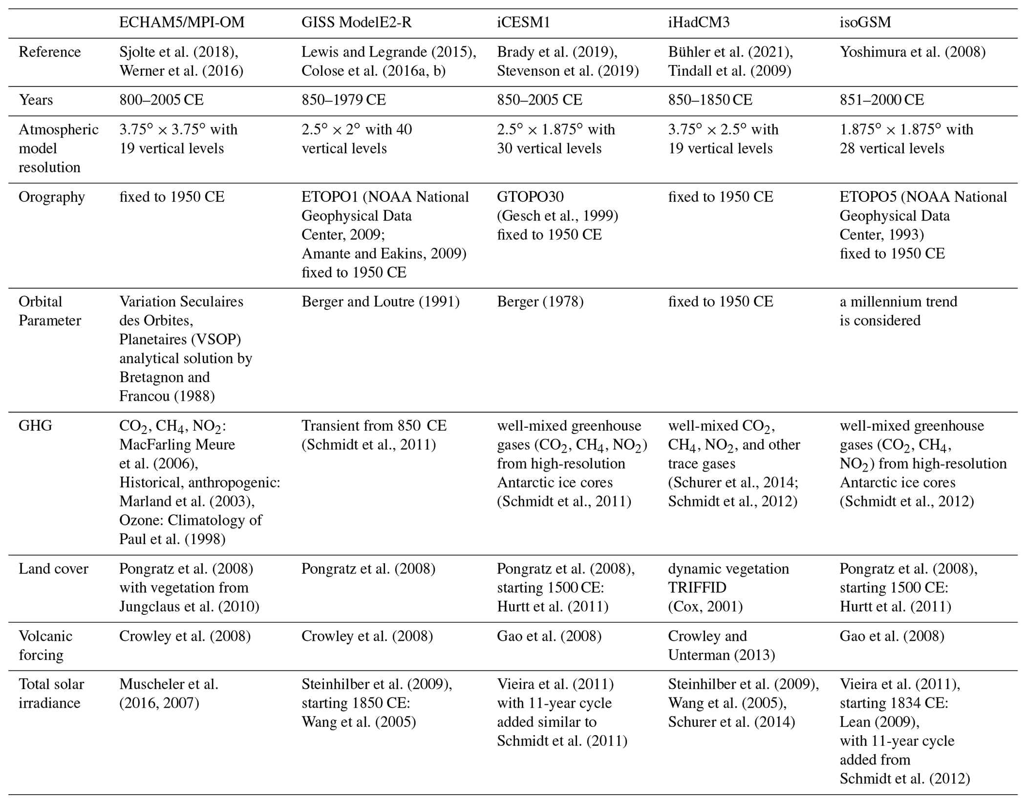
Here we will present a multi-model comparison of five isotope-enabled last millennium simulations: ECHAM5/MPI-OM (Sjolte et al., 2018), GISS ModelE2-R (Lewis and Legrande, 2015; Colose et al., 2016a, b), the isotope-enabled version of the Community Earth System Model (Stevenson et al., 2019; Brady et al., 2019), the isotope-enabled version 3 of the Hadley Model (Bühler et al., 2021), and the stable water-isotope-incorporated Scripps Experimental Climate Prediction Center's Global Spectral Model (Yoshimura et al., 2008), with climate characteristics and forcings as depicted in Fig. 1 and listed in Table 1. This multi-model comparison complements previous work (Jungclaus et al., 2017; Midhun and Ramesh, 2016; Conroy et al., 2013) through its focus on how different models represent SWI and their variability on different timescales over the entire last millennium. We aim to identify common model biases (Kageyama et al., 2018) globally and in different regions, as well as distinguish specific climate drivers for modeled isotope variability on decadal and longer timescales. This allows, for the first time, for the joint intercomparison of SWI variability in climate models and proxy archives in a time period dominated by natural forcing.

The last millennium is a suitable time period for model–data comparisons, as it provides an opportunity to study variability on decadal and longer timescales and to decipher internal from externally forced variability (Kageyama et al., 2018). Boundary conditions such as orbital forcing, sea level, and ice sheets are close to present-day levels, and external variability is mostly driven by variations in volcanic eruptions (Schurer et al., 2014; Neukom et al., 2019; Legrande and Anchukaitis, 2015). It is a key paleoclimate period for the CMIP5 and CMIP6 experiments (Taylor et al., 2012; Eyring et al., 2016), and speleothem records are abundant in this period (Bühler et al., 2021).

With this study, we aim to contribute to the understanding of both model and data by answering the following questions: (a) first, how do different simulations model oxygen isotopes in the hydrological cycle, and how do they compare to archived speleothem data? (b) Second, what processes influence speleothem isotope composition, and what effects of variability can be captured and later analyzed? We first compare their similarities and differences in the isotopic signatures of precipitation both globally (Sect. 4.1) and specifically at the cave site locations of a large number of high-resolution speleothems from the SISALv2 database (Comas-Bru et al., 2020b). Through spatial testing of climate variables, we analyze the relationship between the measured stable isotopes of oxygen and carbon and different modeled climate variables (Sect. 4.2). These relationships will help to determine spatial biases between the models and drivers for modeled and recorded isotopes. Temporal coherence between models and data give insight into internal and externally driven climate variability on different timescales. In a second step, we thus investigate if models can reproduce variability as measured in speleothems on annual to centennial timescales (Sect. 4.3). Finally, we test the timescales of externally forced events, e.g., volcanic eruptions or variations in the solar irradiance, that speleothems archives are able to resolve (Sect. 4.4).

2 Data

In this study, we collected and standardized the output from five different isotope-enabled climate model simulations over the last millennium, as well as oxygen and carbon isotopes in speleothems from the SISALv2 database.

2.1 Isotope-enabled general circulation models

A major advantage given by modeling SWI is its ability to both temporally and spatially resolve the variability of isotopes in precipitation by adding H${}_{\mathrm{2}}^{\mathrm{18}}$O and HDO to the part which already simulates and traces the most abundant stable water isotope, H${}_{\mathrm{2}}^{\mathrm{16}}$O. Simulated δ¹⁸O will further be denoted as δ¹⁸O_sim. In the atmospheric advection scheme of the model, which is generally a part of the model's dynamical core, all three water isotopologues behave identically. In case of a phase transition (such as melting, condensing, evaporating, and freezing), additional fractionation effects are applied to the two less abundant water isotopologues. These phase changes typically occur in evaporation from land and ocean surfaces; condensation during formation of clouds, rain, snow; and re-evaporation of precipitation below cloud (for example, Werner, 2010; Sturm et al., 2010).

The models used in this study range from AGCMs forced with sea surface temperatures and sea ice distribution to atmosphere–ocean general circulation models (AOGCMs). Their basic characteristics and boundary conditions are listed in Table 1. They are both used individually in the analysis and by the ensemble mean of all models. Figure 1 shows the climate as represented by the different models and external forcings used in the simulations. Since SWING2, there has not been a consistent protocol for simulations with isotope-enabled models. Hence, the simulations used in this study largely follow the PMIP version 3 last millennium experiment protocol (Schmidt et al., 2011, 2012) with its proposed climate forcing reconstructions, with some variations in vegetation and orography. Of the external forcings used, differences in the volcanic forcing may have the largest influence on differences between the simulations (Colose et al., 2016a; Schmidt et al., 2011), as different responses on larger eruptions may have a long-term impact. Large eruptions can cause local anomalies to the mean state of δ¹⁸O of up to ±1.5 ‰ (Colose et al., 2016a), hinting at the magnitude of change that can be caused by different forcings. Volcanic eruptions are among the most prominent drivers of natural climate variability during the last millennium (Jungclaus et al., 2017). Compared to volcanic forcing, the choice of solar or orbital forcing has a smaller effect over time in the last millennium. Although the simulations do use forcings based on different reconstructions, which then act on various timescales, differences in response may arise not only from forcings but also from their implementation in the models (Jungclaus et al., 2017).

Figure 1 Climate as represented by the different models (ECHAM5-wiso: light blue; GISS-E2-R: dark blue; iCESM: grey; iHadCM3: green; and isoGSM: orange) and external forcings over the last millennium. (a) Global mean surface temperature anomaly as represented by the models (in model colors) relative to the period of the last millennium (850–1850 CE), the reconstructed temperature anomaly (PAGES2k, red, PAGES2k-Consortium, 2019), and observed temperatures (HadCRUT4, black, Morice et al., 2012). (b) Isotopic composition of precipitation in the different models (in model colors) at the cave site location of Bunker cave (Germany), including the δ¹⁸O_speleo of entity ID 240 (red), all at the temporal resolution of entity ID 240 (Comas-Bru et al., 2020b; Fohlmeister et al., 2012). For both temperature and δ¹⁸O, we show the annual and downsampled values in lighter colors in the background. Bold colors show the values with a 100-year Gaussian kernel bandpass (Rehfeld and Kurths, 2014). (c) Atmospheric CO₂ concentration (SMT: Schmidt et al., 2012; MFM: MacFarling Meure et al., 2006). (d) Volcanic forcing in units of aerosol optical depth (AOD) (CRO: Crowley et al., 2008; Crowley and Unterman, 2013; GAO: Gao et al., 2008), where the AOD for the Gao et al. (2008) reconstruction was estimated by dividing the sulfate loading by 150 Tg (following Atwood et al., 2016). (e) Total solar irradiance (TSI) (STH: Steinhilber et al., 2009, MSL: Muscheler et al., 2016, VR: Vieira et al., 2011). The grey bars mark particular periods of high volcanic forcing.

Sjolte et al. (2018)Lewis and Legrande (2015)Brady et al. (2019)Bühler et al. (2021)Yoshimura et al. (2008)Werner et al. (2016)Colose et al. (2016a, b)Stevenson et al. (2019)Tindall et al. (2009)(Gesch et al., 1999)20091993Amante and Eakins, 2009Berger and Loutre (1991)Berger (1978)1988(Schmidt et al., 2011)2006Schurer et al., 2014Marland et al. (2003)(Schmidt et al., 2011)Schmidt et al., 2012(Schmidt et al., 2012)Paul et al. (1998)Pongratz et al. (2008)Pongratz et al. (2008)Pongratz et al. (2008)Pongratz et al. (2008)Jungclaus et al. (2010)Hurtt et al. (2011)(Cox, 2001)Hurtt et al. (2011)Crowley et al. (2008)Crowley et al. (2008)Gao et al. (2008)Gao et al. (2008)2013Muscheler et al.Steinhilber et al. (2009)Vieira et al. (2011)Steinhilber et al. (2009)Vieira et al. (2011)20162007Wang et al. (2005)Wang et al. (2005)Schurer et al. (2014)Lean (2009)Schmidt et al. (2011)Schmidt et al. (2012)

Table 1 Basic characterization of the last millennium simulation.

2.1.1 ECHAM5/MPI-OM

We use the isotope-enabled version of the fully coupled general circulation models (GCMs) ECHAM5–MPI-OM (hereafter, ECHAM5-wiso) (Werner et al., 2016; Jungclaus et al., 2006). The model consists of the atmospheric model ECHAM5 (Roeckner et al., 2003) and the ocean model MPI-OM with an embedded sea ice model (Marsland et al., 2002). The millennium-long simulation by Sjolte et al. (2018) covers the period 800–2000 CE and uses a similar setup to the E1 COSMOS ensemble by Jungclaus et al. (2010) but with a different solar forcing based on the solar modulation record inferred from combined neutron monitor and tree-ring ¹⁴C data (Muscheler et al., 2016).

Isotope diagnostics have been implemented for the atmosphere, ocean, and land surface component of the model and are computed throughout the entire water cycle in the ECHAM5 (Werner et al., 2016) and MPI-OM (Werner et al., 2016) models. The land surface model assumes no fractionation in most of the physical processes (Haese et al., 2013). Water tracers are fully mixed and advected in the ocean model, and the SWI total mass is conserved (Werner et al., 2016).

ECHAM5-wiso has been used extensively within the paleoclimate field, as well as for modeling of the present climate (for example, Werner et al., 2016; Langebroek et al., 2011; Goursaud et al., 2018). The fully coupled GCM version of the model ECHAM5–MPI-OM has good agreement with both present-day isotope observations from the GNIP database, as well as with ice core and speleothem proxies during mid-Holocene (Comas-Bru et al., 2019), Last Glacial Maximum (Werner et al., 2016; Comas-Bru et al., 2019), and for the last interglacial (Parker et al., 2021). Both in the GCM and with the atmospheric component (ECHAM5-wiso), a warm bias in the model is found over high-latitudinal regions, especially over Greenland and Antarctica (Werner et al., 2011, 2016). This has been attributed to the coarse spatial resolution in the atmospheric component of the model (Werner et al., 2016) resulting in an underestimation of isotope depletion in these regions. The last millennium simulation has not been evaluated globally, but climate reconstructions and variability of SWI have been compared in the North Atlantic region, where the amplitude of the variability was underestimated in the model compared to ice cores (Sjolte et al., 2018). Previous studies also stress the isotopic response to volcanic eruptions and phases of NAO (Guðlaugsdóttir et al., 2018, 2019).

2.1.2 GISS ModelE2-R

The isotope-enabled AOGCM GISS ModelE2-R (hereafter, GISS-E2-R) (Schmidt et al., 2006, 2014) is used with the same physics as in the CMIP5 experiments (Miller et al., 2014; Schmidt et al., 2014). Water tracers and isotopes are incorporated into the atmosphere, land surface, ocean, and sea ice components of the model (Schmidt et al., 2005). Several experiments have been set up for the last millennium with GISS-E2-R due to uncertainties in past forcings and their effects, with different combinations of solar, volcanic, and land use (vegetation) forcings but with the same greenhouse gas and orbital change in every case (Colose et al., 2016a, b; Lewis and Legrande, 2015).

GISS-E2-R has been shown to simulate modern observations of SWI well, except over Antarctica, in terms of changes in convection, clouds, and isotope kinetics (Schmidt et al., 2005). For the last millennium, GISS-E2-R has also explored the isotopic responses to volcanic eruptions in South America (Colose et al., 2016a), to volcanic forcing in relation to the position of the intertropical convergence zone (Colose et al., 2016b), and to ENSO (Lewis and Legrande, 2015). The model has been shown to have a warm sea surface temperature bias and issues in sea ice concentration around Antarctica, related to the transport of the Antarctic Circumpolar Current. In the tropics, a warm bias is also found over land, together with cooler northern midlatitudes (Schmidt et al., 2014).

2.1.3 ICESM1

We use the last millennium run of the isotope-enabled AOGCM iCESM1 version 1.2 model (hereafter, iCESM) (Hurrell et al., 2013; Brady et al., 2019; Midhun et al., 2021), a fully forced simulation out of an eight-member ensemble of different external forcings. As the model is open source and publicly available, it is widely used in the scientific community, and simulations for past (Zhu et al., 2017; Zhang et al., 2012) and present climate exist (Otto-Bliesner et al., 2016).

The model consists of the isotope‐enabled Community Atmosphere Model version 5.3 (iCAM5.3, isotope-enabled version based on Neale et al., 2010), a land model CLM4 (Oleson et al., 2010), a sea ice model, and an ocean component that is based on the isotope-enabled POP2 (Zhang et al., 2017). Isotopes in the water cycle are represented as a new parallel hydrological cycle in all hydrological components in the atmosphere, ocean, land, and sea ice in the form of numerical water tracers and can be tracked in space and time.

The isotope-enabled version captures general global isotopic signatures well over ocean areas but shows small discrepancies across the land surface (Brady et al., 2019). This effect has been explained by the model showing a slight negative isotopic bias due to overestimated modeled convection in mid-latitude oceans. Consequently, the transport of SWI mass poleward and landward has been deemed insufficient (Nusbaumer et al., 2017). Footprints associated with major climatic modes such as ENSO and Pacific decadal oscillation (PDO) are found to also be well represented in isotopic signatures (Midhun et al., 2021).

2.1.4 IHadCM3

We use the last millennium run from the fully coupled isotope-enabled AOGCM iHadCM3 (Bühler et al., 2021). iHadCM3 has been widely used to simulate present (Dalaiden et al., 2020) and future climate (Sime et al., 2008; Tindall et al., 2009; IPCC, 2013), as well as for past climates (Tindall et al., 2010; Sime et al., 2013; Holloway et al., 2018). The model consists of several components: the atmosphere model HadAM3 (Pope et al., 2000), the ocean model HadOM3 (Gordon et al., 2000), a sea ice model (as described in Valdes et al., 2017) and a dynamic land surface and vegetation model (Cox, 2001).

For the isotope-enabled version, SWI were added as two separate water species in the atmospheric model, and as tracers in the ocean model. Fixed isotope fractions are added to a fixed volume grid box of the ocean and experience changes due to evaporation, precipitation, and runoff through a virtual flux of SWI, altering the δ¹⁸O_sim ratio in the top level of the ocean accordingly (Tindall et al., 2009).

Compared to instrumental observations, the model represents sea surface temperature, ice sheet, and ocean heat content well (Gordon et al., 2000). The freshwater hydrological cycle in the model shows only a slight overestimation in the local evaporation (Pardaens et al., 2003). The model simulates the major isotopic fractionation effects defined by Dansgaard (1964) (e.g., the latitude effect, the amount effect, and the continental effect) appropriately compared to GNIP data (Zhang et al., 2012). Additionally, a broad agreement in isotopic output with GNIP data in the general spatial distribution can be observed (Tindall et al., 2009).

2.1.5 IsoGSM

IsoGSM is the isotope-enabled version of the AGCM Scripps Experimental Climate Prediction Center's (ECPC) Global Spectral Model (hereafter, isoGSM) (Yoshimura et al., 2008). The model is based on the previous medium-range forecast model used at NCEP, making it well documented in its performance as an operational weather forecast model (Kanamitsu et al., 2002; Caplan et al., 1997).

The IsoGSM is a standalone atmospheric model. Here, it has been forced with sea surface temperatures and sea ice distributions from the CCSM4 last millennium simulation (Landrum et al., 2013). Land surface processes are modeled through the NOAH model, but isotopic fractionation is not considered in these processes (Yoshimura et al., 2008).

IsoGSM has shown to represent isotope and precipitation observations globally using a spectral nudging technique captured by the NCEP–DOE Reanalysis dataset (Yoshimura et al., 2008). Its last millennium simulation has not been evaluated in previous studies, but isoGSM captures large-scale isotope and climate patterns in present times (Risi et al., 2012). The model has been shown to also reproduce observed isotopic and precipitation variability well over the regions of Indian summer monsoon (Berkelhammer et al., 2012a), western North America (Berkelhammer et al., 2012b), and northwestern Scotland (Baker et al., 2012). Recently, IsoGSM showed good consistency with speleothem oxygen isotopes from East Asia (Chiang et al., 2020) and from South Asia (Kathayat et al., 2021). IsoGSM tends to underestimate the depletion of δ¹⁸O_sim in dry regions such as Antarctica (Yoshimura et al., 2008). A decreasing summer temperature increases the precipitation δ¹⁸O_sim and is caused by the moisture transport scheme of the model associated with areas of extremely dry conditions (Yoshimura et al., 2008; Risi et al., 2012).

2.2 SISALv2 database

In this study, we use speleothem data from the Speleothem Isotope Synthesis and Analysis version 2 (SISALv2) database (Atsawawaranunt et al., 2018; Comas-Bru et al., 2019; Comas-Bru et al., 2020a, b). The database includes 691 speleothem records from 294 caves across the globe from all continents except Antarctica. Globally, the last millennium has abundant records with sufficient resolution and reasonable dating uncertainties (Bühler et al., 2021). We filtered the database for records that cover at least a 600-year period within the last millennium (850–1850 CE) and exhibit at least 2 dates and 36 stable isotope measurements within the time period to guarantee a minimum resolution of 30 years. We obtain 89 records from 75 different sites for δ¹⁸O_speleo, of which 58 records (65 %) from 50 sites also have δ¹³C_speleo measurements (Fig. 2).

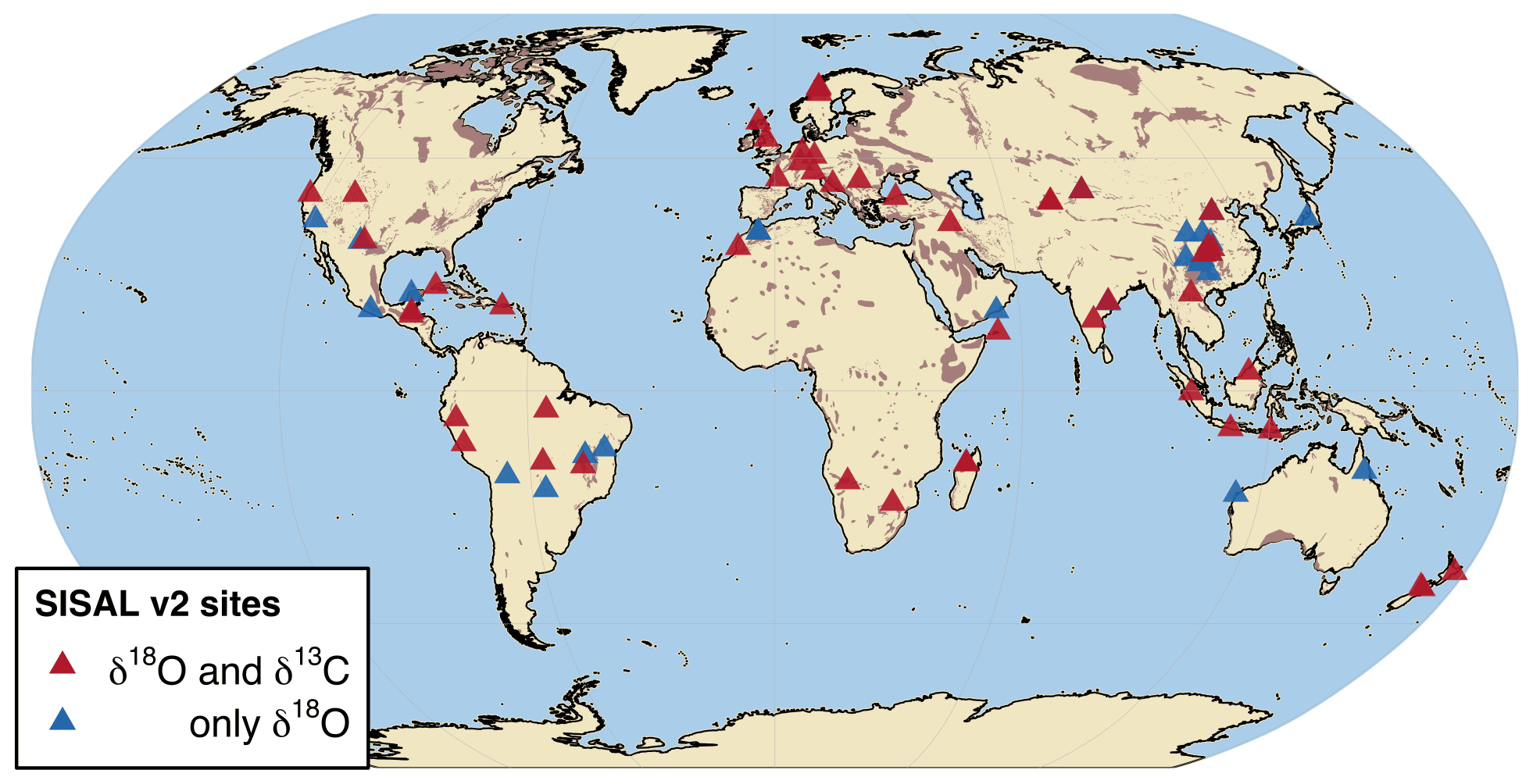
Figure 2 Site locations of the SISALv2 database on a global karst map (brown shading by Williams and Ford, 2006). We only consider entities that cover a minimum 600-year period within the last millennium and that include at least 2 dates and 36 isotopic measurements in this period. Shown are all sites within the last millennium meeting these selection criteria that have both oxygen and carbon isotope measurements (red) and only oxygen isotope measurements (blue).

3 Methods

To compare climate simulation outputs and speleothem data, both need some preparation. Modeled output comes in regular monthly resolution, while time series of speleothem proxies are irregularly sampled. Different speleothem mineralogies, as well as different isotopic standards between modeled and recorded data, need to be accounted for before statistical similarity measures are applied.

3.1 Speleothem drip water conversion

The database includes calcite, aragonite, and mixed mineralogy speleothem records. Following Comas-Bru et al. (2020b), we only use pure calcite or aragonite speleothems in our analysis. Stable isotope ratios are usually given in δ notation, with stable oxygen isotopes given as ${\mathit{\delta }}^{\mathrm{18}}\mathrm{O}=(\frac{\frac{{}^{\mathrm{18}}\mathrm{O}}{{}^{\mathrm{16}}{\mathrm{O}}_{\mathrm{sample}}}}{\frac{{}^{\mathrm{18}}\mathrm{O}}{{}^{\mathrm{16}}{\mathrm{O}}_{\mathrm{standard}}}}-\mathrm{1})\cdot \mathrm{1000}$ ‰, with the standard denoting either the Vienna Standard Mean Ocean Water (V-SMOW, Dansgaard, 1964; Kendall and Caldwell, 1998) for water in its liquid and gaseous phases, or Vienna Pee Dee Belemnite (V-PDB, Coplen et al., 1983) for CaCO₃. The stable carbon isotope ratio is denoted as ${\mathit{\delta }}^{\mathrm{13}}\mathrm{C}=(\frac{\frac{{}^{\mathrm{13}}\mathrm{C}}{{}^{\mathrm{12}}{\mathrm{C}}_{\mathrm{sample}}}}{\frac{{}^{\mathrm{13}}\mathrm{C}}{{}^{\mathrm{12}}{\mathrm{C}}_{\mathrm{standard}}}}-\mathrm{1})\cdot \mathrm{1000}$ ‰ against the V-PDB (Coplen, 1995).

To be able to compare precipitation δ¹⁸O_sim values to those measured in calcite or aragonite, the δ¹⁸O_speleo is converted to its drip water equivalent (δ¹⁸O_dweq) relative to the V-SMOW standard as in Comas-Bru et al. (2019). This conversion is temperature dependent to different extents for both minerals. Tremaine et al. (2011) provide an empirically based fractionation formula for speleothems of calcite mineralogy:

$$\begin{array}{}\text{(1)}& {\mathit{\delta }}^{\mathrm{18}}{\mathrm{O}}_{\mathrm{dweq}}={\mathit{\delta }}^{\mathrm{18}}{\mathrm{O}}_{\mathrm{calcite}}-\left(\right({\displaystyle \frac{\mathrm{16.1}\cdot \mathrm{1000}}{T}})-\mathrm{24.6}),\end{array}$$

where T is the temperature in K and δ¹⁸O are given in units of ‰.

Aragonite speleothems form under different conditions, e.g., higher Mg content of the dripping solution or slow drip rate (Fairchild and Baker, 2012), resulting in a different fractionation factor compared to calcite as described by Grossman and Ku (1986):

$$\begin{array}{}\text{(2)}& {\mathit{\delta }}^{\mathrm{18}}{\mathrm{O}}_{\mathrm{dweq}}={\mathit{\delta }}^{\mathrm{18}}{\mathrm{O}}_{\mathrm{aragonite}}-\left(\right({\displaystyle \frac{\mathrm{18.34}\cdot \mathrm{1000}}{T}})-\mathrm{31.954}).\end{array}$$

For both conversions, the cave temperature at the time of the fractionation is needed. As these are often not available, especially in a paleoclimate setting, we use annual mean modeled surface temperatures as a surrogate for cave temperatures (Fairchild and Baker, 2012). For caves in very cold conditions, the annual mean surface temperature may underestimate the mean cave temperature by some degrees due to long-lasting snow packs. This underestimation, however, only corresponds to an overestimation of 1 ‰ in δ¹⁸O_dweq and is within the range of the simulation ensemble. Additionally, cave-dependent time lags between the surface and the cave temperature are not accounted for, as they have a negligible effect on the time-averaged mean isotopic value. The conversion to drip water equivalent is done for each entity and each simulation individually, where we use the simulated annual mean surface temperature, downsampled to the record's resolution.

In a last step, the V-PDB values are converted to V-SMOW for direct comparison to the modeled SWI, using the conversion from Coplen et al. (1983):

$$\begin{array}{}\text{(3)}& {\mathit{\delta }}^{\mathrm{18}}{\mathrm{O}}_{\mathrm{SMOW}}=\mathrm{1.03092}\cdot {\mathit{\delta }}^{\mathrm{18}}{\mathrm{O}}_{\mathrm{PDB}}+\mathrm{30.92}.\end{array}$$

For carbon isotopes, different fractionation paths exist depending on mineralogy. Following Fohlmeister et al. (2020), we convert the aragonite δ¹³C values to corresponding calcite values using a fractionation offset of 1.9±0.3 ‰ $({\mathit{\delta }}^{\mathrm{13}}{\mathrm{C}}_{\mathrm{c}}={\mathit{\delta }}^{\mathrm{13}}{\mathrm{C}}_{\mathrm{calcite}}={\mathit{\delta }}^{\mathrm{13}}{\mathrm{C}}_{\mathrm{arag}}-\mathrm{1.9}\pm \mathrm{0.3}\mathrm{‰})$. This offset accounts for the different enrichment factors of the two polymorphs as established in laboratory studies (Romanek et al., 1992) and confirmed in a speleothem study (Fohlmeister et al., 2018).

From the drip water conversion, we obtain a matrix for each of the isotopes with one row per measurement and six columns, where one represents the observations and the other five the modeled estimates.

3.2 Data processing

The simulation output from the five different climate models is available at monthly resolution but with differing time coverage. All simulation runs are cut to cover the time period from 850 to 1850 CE, an interval that is similar to PMIP's interval in the last millennium experiment. We focus on surface temperature, precipitation, precipitation δ¹⁸O_sim, and evaporation. For the simulations lacking evaporation as a diagnostic (iCESM, isoGSM, and iHadCM3), we convert latent heat to potential evaporation and use these variables within the simulations. Outliers in the simulation are removed by comparing each modeled value in the 3D-output data matrix with its eight neighbors in time and space. If the value deviates from the mean of these eight values by more than five standard deviations, the value is set to NA. On average 0.001 % of values are set to NA through this method.

δ¹⁸O_speleo forms from drip water that reaches the cave, which can be approximated by calculating the difference between precipitation amount and evaporation. When comparing modeled to speleothem isotopes it is therefore more realistic to weight the modeled δ¹⁸O_sim by precipitation minus evaporation amount (infiltration-adjusted precipitation weighting, iw) to obtain annual δ¹⁸O_sim values. The weighting automatically focuses on the local seasonal composition of SWI in rainfall, and prevents bias towards seasons with minimal infiltration due to high evaporation. Weighted δ¹⁸O_sim values are commonly used in speleothem model–data comparison studies (Comas-Bru et al., 2019; Baker et al., 2019). The simulated weighed δ¹⁸O mean is calculated as follows:

$$\begin{array}{}\text{(4)}& {\mathit{\delta }}^{\mathrm{18}}{\mathrm{O}}_{\text{iw}}={\displaystyle \frac{{\sum }_{\mathrm{1}}^n{{\mathit{\delta }}^{\mathrm{18}}\mathrm{O}}_k{\text{iw}}_k}{{\sum }_{\mathrm{1}}^n{\text{iw}}_k}},\end{array}$$

where δ¹⁸O_iw is the monthly weighted annual composition of isotopes, δ¹⁸O_k refers to monthly simulated δ¹⁸O, and iw_k is the corresponding monthly amount of iw, where n=12. As isotopic fractionation also occurs during evaporation from the soil, models where δ¹⁸O_sim is also available for soil layers would be more realistic to compare to speleothem data. However, these were only available for a few simulations. Using δ¹⁸O_sim of precipitation for the calculation of δ¹⁸O_iw therefore offered a more equal handling of the data while maintaining the large ensemble and enabled a better comparison of results.

Where simulation data are compared on a grid box level, we block average all simulations to the same spatial resolution as that of the ECHAM5-wiso run, which has the lowest spatial resolution. Data at the speleothem cave sites are extracted via bilinear interpolation as in Bühler et al. (2021). Here, a grid box of the size of the simulation's original resolution with the cave's location at its center is resampled from the original grid boxes it overlaps with. We note that this bilinear interpolation can, however, influence the temporal variability or the values of the response variables (Latombe et al., 2018).

The simulated monthly temperature, precipitation, and evaporation at the speleothem cave locations are averaged to annual mean values. All speleothems in our last millennium subset, however, come as irregularly sampled time series with a median resolution of 5.19 years per entity (90 % CI: 4.13, 6.99). Considering only the speleothems with measurements of both isotopes yields a median resolution of 6.08 years (4.07, 7.85). To adjust the model and speleothem data, the simulated variables of all models are block averaged to the irregular temporal resolution of the individual speleothem. We also include speleothems in our analysis where no δ¹³C measurements, but only δ¹⁸O data are available. In direct comparisons between carbon and oxygen isotopes, we only consider those 58 speleothems that provide samples for both isotopes.

The relationship between δ¹⁸O_speleo and simulated climate variables is determined following three different latitude bands to guarantee enough data points within each climate zone, the tropics, the subtropics, and the extratropics (Holden, 2012). The tropics are commonly defined as the zone between the Tropic of Cancer and the Tropic of Capricorn (23.44^∘ S to 23.44^∘ N), the subtropical region is defined as 23.44–35^∘ N/S, and the extratropical region is defined as 35–90^∘ N/S (with cave sites only extending to 66^∘ N and 42^∘ S).

Spatial testing between speleothem δ¹⁸O_dweq, δ¹³C_c, simulated δ¹⁸O_iw, and meteorological variables is done by linear regression of the simulated millennium mean, downsampled to the temporal resolution of each record, and entity mean. To account for the spread between simulated variables and calculated δ¹⁸O_dweq, the linear regression is done via bootstrapping (n=2000). Confidence intervals for all entity mean variables are also calculated via bootstrapping with a significance level of α=0.1. The p values are calculated through a fit linear regression model (fitlm.m, MATLAB, 2018) using Pearson’s product moment correlation.

Correlation estimates and p values for regular time series, i.e., the annual resolution output of the simulation, are calculated via the Pearson's product moment correlation (via the function cor.test, R Core Team, 2020). We use a significance level of α=0.1.

Correlation estimates for irregular time series are calculated via Pearson correlation as adapted by Rehfeld and Kurths (2014) and tested for last millennium speleothem records in Bühler et al. (2021). Here, we also choose a significance level of α=0.1. This level is appropriate for both the regular and irregular time series, considering the number of samples N compared to the strictness and expected level of false positives. Whenever calculating correlation estimates where speleothem data is involved, we use the raw δ¹⁸O_speleo or δ¹³C_speleo instead of the converted drip water values to decrease any potential biases.

With all simulated variables downsampled to the irregular resolution of each speleothem record, the use of power spectral analysis of the time series can describe the variation of common signals on a frequency spectrum of all time series (Chatfield, 2003). The power spectral density (PSD) of a time series describes the power distribution versus frequency over a finite interval of time (Chatfield, 2003).

To compute spectra of irregularly sampled time series, these are first interpolated to their mean resolution by a double interpolation and filtering process (following Laepple and Huybers, 2014a; Rehfeld et al., 2018; Dolman et al., 2021). This interpolation is performed to reduce high-frequency artifacts. The robustness of this spectral estimation process was recently confirmed by Hébert et al. (2021).

3.3 Synchronous extreme events in speleothem isotopes

An alternative similarity measure to correlation estimates, especially given the irregularity of the available time series, is checking for synchronous extreme events within two time series. After distinguishing extreme events, strength and direction of synchronous extreme events are only based on their relative timing (Rehfeld and Kurths, 2014). In this study, we only focus on the relative timing of the distinguished extreme events to each other.

Within the modeled or measured isotope time series, we distinguish the 5 % extreme values as the values above or below the 97.5 % or 2.5 % quantile of the time series distribution, respectively. Two extreme values occurring in a row are treated as two separate extreme events. Extreme values for time series of solar irradiance are determined in the same manner. For the volcanic forcing time series, we distinguish those events above the 95 % quantile of the distribution.

Two events are considered synchronous if they both occur within a time period around the events limited by a local threshold τ. This local threshold is calculated for each possible pair of extreme events and is chosen as half the minimum time between either extreme event and its preceding or succeeding extreme. For our dataset, the median τ is 4.62 years (90 % CI: 4.37, 5.28), which is of the same order of magnitude as the median resolution of all records with both carbon and oxygen measurements of 6.08 years, (4.07, 7.85). We set a hard threshold limit of 50 years, corresponding to the median age uncertainty considering the original chronologies and the SISALv2 ensemble chronologies (Comas-Bru et al., 2020b). When comparing synchronous events between isotopes within one particular speleothem, age uncertainties are negligible in the comparison as δ¹³C_speleo and δ¹⁸O_speleo values stem from the same measurement of individual sub-samples.

For comparable extreme event signatures between the modeled and measured isotopes to volcanic or solar forcings, each modeled time series is checked for synchronicity against their respective forcing time series. The analysis is repeated for the speleothems for the same number of forcings and averaged.

When looking at the temporal distribution of global synchronous extreme events, they are sorted into bins of 10 years, which is approximately twice the median local τ. If a pair shows several extreme events within one bin, it is only counted once. We determine significance by randomly permuting one of the time series of a pair and repeating the analysis 2000 times. Within one bin, all counts that are larger than the 95 % quantile of this “mean background noise” can be regarded as significant.

4 Results

4.1 Overview of simulated versus measured speleothem oxygen isotopes

We first compare the mean δ¹⁸O_iw signal of the five different last millennium simulations to see potential model biases and large differences between the simulations (Figs. 3 and S1 in the Supplement). The global mean δ¹⁸O_iw values are fairly similar in area-weighted global mean of −8.48 ‰ (90 % CI: −8.61, −8.36) and −8.41 ‰ (−8.62, −8.2) for isoGSM and GISS-E2-R, respectively. The ECHAM5-wiso run is less depleted with a global δ¹⁸O_iw mean of −7.27 ‰ (−7.46, −7.09) and with visibly less depleted mid-latitude oceans than in the other simulations. The iCESM and iHadCM3 data show a stronger depletion of −9.39 ‰ (−9.51, −9.28) and −9.15 ‰ (−9.29, −9.01) respectively, with iCESM showing stronger depletion in the mid-latitudes and iHadCM3 showing stronger depletion towards the Antarctic compared to the other simulations. Although GISS-E2-R shows strong depletion, especially in the Arctic region, the less depleted mid-latitudes dominate the global mean (see Fig. S1).

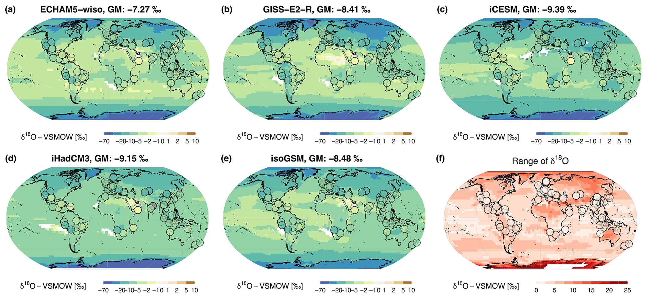
Figure 3 Simulated δ¹⁸O_iw climatology (a–e) of the respective simulation: (a) ECHAM5-wiso, (b) GISS-E2-R, (c) iCESM, (d) iHadCM3, and (e) isoGSM in the background. The time-averaged mean δ¹⁸O_dweq values using the respective simulated temperatures are depicted as circles. Global means (GM) of δ¹⁸O_iw are given in the title of each subplot. (f) The range of δ¹⁸O_iw between all simulations for each grid box, as well as the range for the difference between simulation and record. Light colors indicate large agreement between the simulations, while darker colors mark areas where the models differ strongly and the spread between the δ¹⁸O_iw is larger. Antarctic δ¹⁸O_iw ranges are up to 40 ‰, highlighting the different model performance in this region (white area in f).

This general offset between the global mean δ¹⁸O_iw is also visible when comparing the spread of mean values on a grid box level (Fig. 3f), where isotopic signatures differ the most strongly in the Antarctic. Restricting the view to low latitudes and mid-latitudes, the largest model data differences are found in the Sahara, the Arabian Peninsula, the Indian subcontinent, and Siberia, where low humidity, high-precipitation amount, or high continentality are the driving local forces of precipitation δ¹⁸O. Also shown in Fig. 3f) is the spread between the offsets to the respective δ¹⁸O_dweq at the cave locations. A close agreement between the models does, however, not necessarily indicate a good model–data match. It only indicates that the differences between the converted speleothem data are similar in the models. The highest agreement of 2.31 ‰ is obtained at Tham Duon Mai cave in Laos (siteID 293 at 20.75^∘ N, 102.65^∘ E, Wang et al., 2019), while the strongest disagreement of 8.14 ‰ between simulations is at Huangye cave in China (siteID 17 at 33.58^∘ N, 105.11^∘ E, Tan et al., 2011).

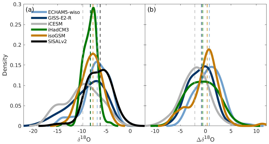
Figure 4 Kernel density estimates of (a) the general distributions in simulated and speleothem δ¹⁸O at cave locations and (b) differences between simulations and the speleothem last millennium mean $(\mathrm{\Delta }{\mathit{\delta }}^{\mathrm{18}}\mathrm{O}={\mathit{\delta }}^{\mathrm{18}}{\mathrm{O}}_{\mathrm{iw}}-{\mathit{\delta }}^{\mathrm{18}}{\mathrm{O}}_{\mathrm{dweq}})$. Dashed lines represent the median.

Analyzing the differences between simulations and speleothems can indicate how well the model data matches the proxy signal. Here we investigate the differences in δ¹⁸O between simulated last millennium mean (δ¹⁸O_iw) and speleothems $(\mathrm{\Delta }{\mathit{\delta }}^{\mathrm{18}}\mathrm{O}={\mathit{\delta }}^{\mathrm{18}}{\mathrm{O}}_{\mathrm{iw}}-{\mathit{\delta }}^{\mathrm{18}}{\mathrm{O}}_{\mathrm{dweq}})$ on a global scale through general distributions, where disagreements between each model and speleothem data are shown as kernel density estimates (Fig. 4). The full datasets are acknowledged through the mean value, whereas the median values exclude skewed distributions and extremes. The speleothem dataset has a median general distribution of −6.21 ‰ globally. Of the simulations, ECHAM5-wiso has the closest distribution median with −6.82 ‰, followed by isoGSM (−7.72 ‰), iHadCM3 (−8.20 ‰), GISS-E2-R (−8.25 ‰), and iCESM (−9.79 ‰) (Fig. 4a). The distributions between simulations and speleothem δ¹⁸O (Fig. 4b) are fairly symmetrical but vary between the simulations, with medians of 0.72 ‰, −0.86 ‰, −2.01 ‰, −0.67 ‰, and 0.28 ‰, for ECHAM5-wiso, GISS-E2-R, iCESM, iHadCM3 and isoGSM, respectively. While ECHAM5-wiso has the closest median globally, isoGSM has the smallest difference between simulation and speleothem δ¹⁸O at cave locations, with a mean of −0.17 ‰ (90 % CI: −0.66, 0.33). GISS-E2-R and iCESM have more negative differences, with a mean of −1.02 ‰ (−1.41, −0.62) and −2.04 ‰ (−2.50, −1.60) respectively, followed by iHadCM3 −0.68 ‰ (−1.18, −0.18). ECHAM5-wiso is the only model that has a mean positive difference between simulation and speleothem data, with a mean of 0.63 ‰ (0.20, 1.05), in line with the less depleted global mean seen in Fig. 3.

The largest positive difference (less depleted δ¹⁸O_iw than δ¹⁸O_dweq) is found at Huagapo cave in Peru (siteID 277 at 11.27^∘ S, 75.79^∘ W, Kanner et al., 2013) and Minnetonka cave in the USA (siteID 200 at 42.09^∘ N, 111.52^∘ W, Lundeen et al., 2013) for at least four model simulations. The highest negative difference (at least three models agree) are found at Hoq cave on Socotra Island, Yemen (siteID 253 at 12.59^∘ N, 54.35^∘ E, Van Rampelbergh et al., 2013), Diva cave in Brazil (siteID 38 at 12.38^∘ S, 41.57^∘ W, Novello et al., 2012), and Qunf cave in Oman (siteID 159 at 17.16^∘ N, 54.30^∘ E, Fleitmann et al., 2007).

The general patterns of the isotope climatology are similar between the models (Fig. 3) but can differ at cave locations (Fig. S2). Larger differences in the modeled isotopic signatures appear particularly in regions where modeled temperature also spreads widely. On average, the differences to the speleothem records (Fig. 4) appear small and are consistent with the general difference in precipitation δ¹⁸O_iw.

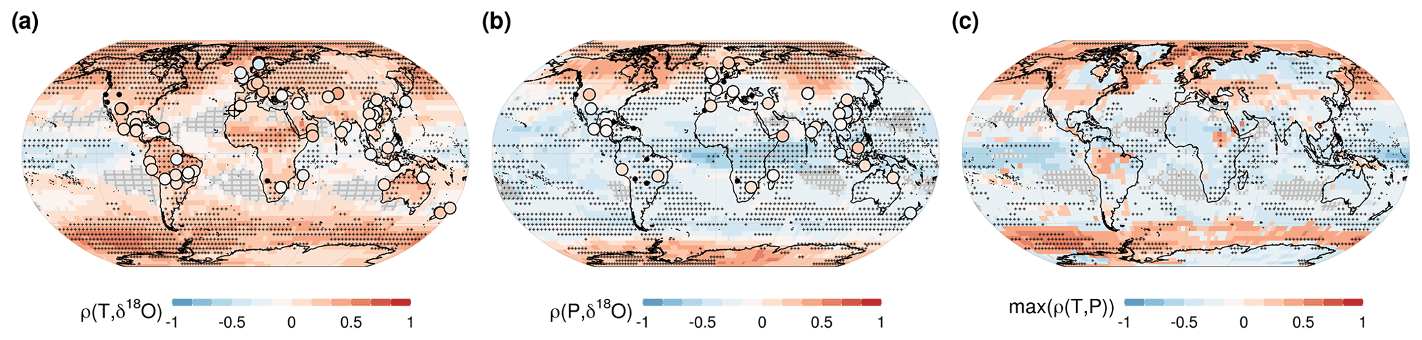
Figure 5 Correlations between SWI and modeled temperature (a) and precipitation (b) time series in each grid box. The background shows the average over all five simulation correlation estimates between annual δ¹⁸O_iw and simulated annual temperature per grid box (a) and for precipitation (b). Crosses indicate grid boxes where correlation estimates for four or more models have the same sign as the averaged estimate over all simulations. Symbols indicate the mean correlation of the simulated temperature (precipitation) of all model simulations to the recorded δ¹⁸O_speleo at record resolution. Crossed circles mark sites where more than four models agree in the mean sign of the correlation to δ¹⁸O_speleo. Black circles indicate the location of those speleothems in the last millennium subset that show no significant correlation to any model. In (c) the map shows positive correlation estimates where $\left|\mathit{\rho }\right({\mathit{\delta }}^{\mathrm{18}}\text{O},\text{T}\left)\right|$ is larger than $\left|\mathit{\rho }\right({\mathit{\delta }}^{\mathrm{18}}\text{O},\text{P}\left)\right|$ (and vice versa for negative values).

Differences between δ¹⁸O_iw signatures between the models may arise from different simulation drivers for the oxygen isotopes, e.g., temperature and precipitation, and can hint at different processes that govern the isotopic water cycle at a certain region within the simulations. The mean of the correlation to these main climatic drivers to δ¹⁸O_iw shows high agreement between the simulations (Fig. 5, individual correlation fields in Fig. S3). For the correlation to temperature (Fig. 5a), two main domains can be distinguished: there is mainly a positive correlation to temperature in the mid-latitudes to high latitudes and on the continents and negative correlation in the low-latitude ocean. Large-scale agreement between the simulations is, however, limited to the higher latitudes and the tropical ocean.

Two domains are also apparent in the correlation to precipitation (Fig. 5b), which are even more clearly separated than for temperature. We find areas of negative correlation to δ¹⁸O_iw in the low latitudes to mid-latitudes and areas of positive correlation only in the high latitudes. The agreement between the simulations, indicated by the crosses, is higher in the low- to mid-latitudes. Combining the information of dominant drivers of δ¹⁸O_iw (absolute higher correlation per grid box in Fig. 5c), we see clear domains of temperature dominance in the Southern Ocean, the higher northern latitudes and some continental regions, while precipitation is more dominant in the lower latitudes, the Antarctic, and Greenland.

The inter-model comparison shows more agreement in the correlation fields to temperature than to precipitation when focusing only on cave locations: the sign of correlation between δ¹⁸O_iw and simulated temperature agrees for three or more simulations at 60 % of locations and for four or more simulations at 26 % of locations. For precipitation, only 11 % of locations agree in sign for three or more simulations and only 1.1 % with agreement in four or more simulations. The more uniform temperature response to external forcing may increase the total number of significant correlation estimates and thus also the number of locations that agree in sign.

The model–data comparison shows more significant temporal correlation estimates between simulated temperature to δ¹⁸O_speleo and also more sign agreement between these correlation estimates than to simulated precipitation. For precipitation, we find no cave, where more than four models agree in the sign to the mean correlation between modeled and recorded δ¹⁸O. For temperature, four speleothems from four different cave sites show a significant correlation of absolute strength $\left|c\right|>\mathrm{0.15}$ for at least four simulations.

The data suggests that two main drivers for δ¹⁸O can be distinguished in specific regions – temperature is dominant in the high latitudes, while precipitation appears to be the main driver in the low latitudes. This is what we expected following the principles established by Dansgaard (1964).

4.2 Spatial testing for climatic and environmental effects on speleothem δ¹⁸O and δ¹³C

The δ¹⁸O in precipitation shows global signatures depending on latitude or altitude amongst other variables (Dansgaard, 1964). We assess this by looking at the relationships between speleothem δ¹⁸O_dweq and δ¹³C_c with the site-specific variables of latitude and altitude.

The δ¹⁸O_dweq decreases as more northern speleothems are considered (hemispherically: Fig. 6a; globally: R²=0.22, p<0.00, Table S1 in the Supplement). The large spread in the mid-latitude Northern Hemisphere is mostly due to the high number of speleothem records available in both Europe and China, implying a high longitudinal spread within the database. Figure 6b shows a global negative relationship of δ¹⁸O_dweq to altitude, even though records get scarcer as the altitude increases. No clear pattern is visible for δ¹³C_c, and the dataset has a large mean spread (Fig. 6c). A statistically significant relationship between altitude and δ¹³C_c cannot be established. However, the spread in δ¹³C_c appears to increase with increasing altitude (Fig. 6d), although under decreasing data density.

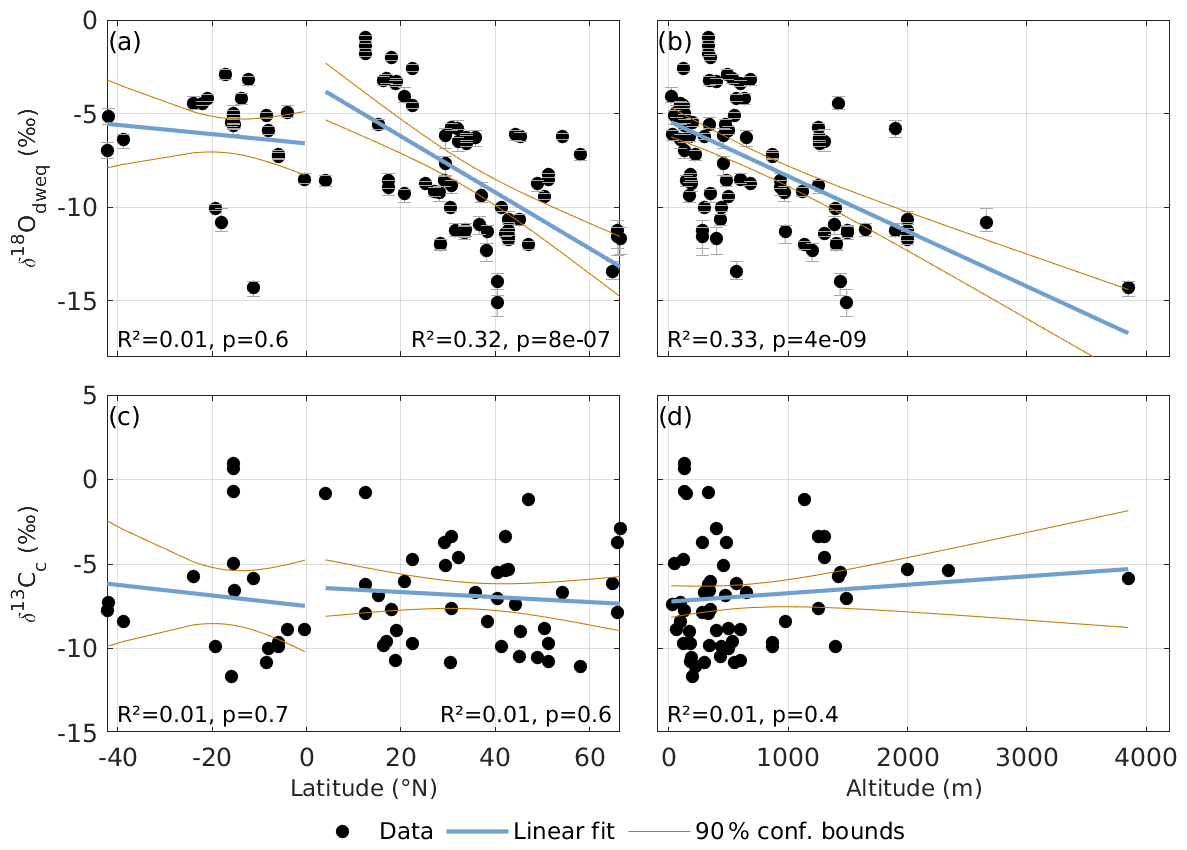
Figure 6 Speleothem δ¹⁸O_dweq (a, b) and δ¹³C_c (c, d) against latitude (a, c) and altitude (b, d) as provided by the SISALv2 database. Linear regression lines are shown separately for both the Northern Hemisphere and Southern Hemisphere in panels (a) and (c) with their respective the R² and p values. In panels (b) and (d), R² and p values correspond to the respective linear regressions across all latitudes. Confidence bounds are 90 %.

We further explore the simulated meteorological variables and investigate spatial relationships between mean δ¹⁸O_speleo and model variable ensemble mean (Fig. 7, Table S1). We find a significant relationship between δ¹⁸O_iw and speleothem δ¹⁸O_dweq across all latitude bands (Fig. 7a–c), with the strongest correlation in the extratropics. Furthermore, we find a global dependency of δ¹⁸O_dweq to mean simulated temperature and precipitation at the cave sites. For both temperature and precipitation, we find the strongest relationships to δ¹⁸O_dweq in the subtropical regions. In all three regions, the relationship to temperature always exceeds that of precipitation. In Fig. 7d–f cave site altitude information is applied by color codes. This helps in the interpretation of possible overlapping effects of temperature and altitude on δ¹⁸O. A significant relationship to annual evaporation can only be distinguished in the extratropical regions (Fig. 7j–l).

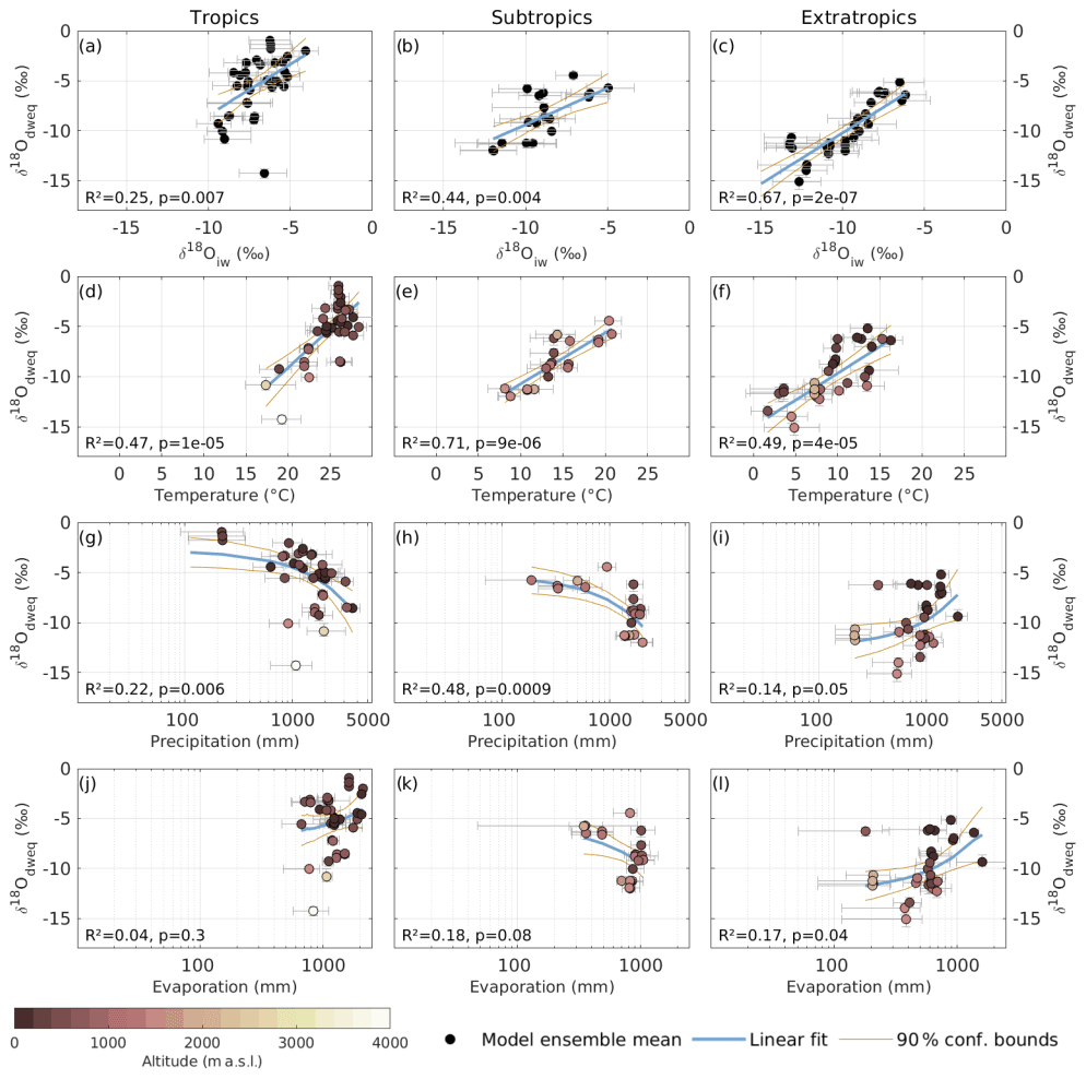
Figure 7 Simulated weighted δ¹⁸O_iw (a–c), temperature (d–e), precipitation (g–i), and evaporation (j–l) against speleothem δ¹⁸O_dweq for model ensemble mean in the tropics, subtropics, and extratropics. The tropical region (23.44^∘ S to 23.44^∘ N) is shown in panels (a), (d), (g), and (j); the subtropical region (23.44–35^∘ N/S) is shown in panels (b), (e), (h), and (k); and the extratropical region (35–90^∘ N/S) is shown in panels (c), (f), (i), and (l). Altitude information is applied as shaded colors in panels (d)–(l). We use δ¹⁸O_iw for all simulations. Note the semi-logarithmic axes for precipitation and evaporation.

We further compare the same meteorological variables to the speleothem δ¹³C_c data (Fig. 8, Table S1). A significant relationship is only found with temperature in the extratropical region (Fig. 8c), with increasing temperatures corresponding to more depleted δ¹³C_c. The δ¹³C_c is also found to be enriched with altitude (R²=0.23, p<0.02, Fig. S4) in the extratropics. This δ¹³C–altitude relationship is not found in the other latitudinal bands.

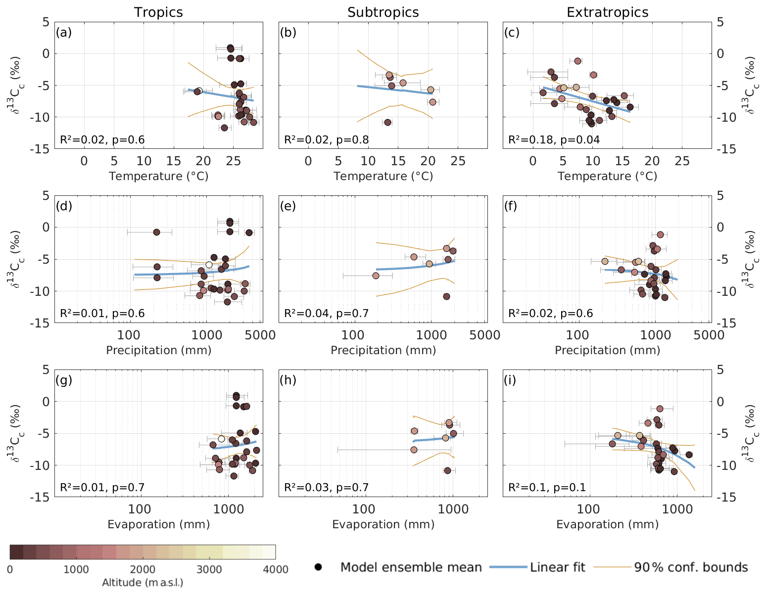
Figure 8 Climate dependence of carbon isotope variability. Shown are simulated ensemble-mean temperature (a–c), precipitation (d–f), and evaporation (g–i) plotted against speleothem δ¹³C_c. Altitude information is applied as shaded colors in (d)–(i). We used linear regressions in all plots; however, these appear curved in a semi-logarithmic plot as used for precipitation and evaporation.

The spatial testing shows globally strong relationships between δ¹⁸O_dweq to environmental factors, in particular to altitude, temperature, and precipitation, which is in line with previous studies (for example, Comas-Bru et al., 2019; Baker et al., 2019). The spatial relationships between speleothem entity mean δ¹³C_c and meteorological variables from model ensemble mean (Fig. 8) only show clear relationships in the extratropical region and not on a global scale. This indicates more local influences as discussed by Fohlmeister et al. (2020).

4.3 Variability on different timescales

We compare the variance distribution in oxygen and carbon isotopes over all speleothems. This is a useful measure of how climatic and environmental factors influence the proxies to a different extent. Additionally, different simulations have different representations of variability across different timescales. This behavior can be explored by calculating power spectral densities (PSD) of the simulated and recorded isotopes averaged globally.

Figure 9 Spectral ratios of isotopes in speleothem and simulations on different timescales as shown by the ratios or mean power spectral densities (PSDs). (a) Spectral ratio between speleothem isotopes (${\mathit{\delta }}^{\mathrm{18}}\mathrm{O}/{\mathit{\delta }}^{\mathrm{13}}\mathrm{C}$). (b–c) Spectral ratio over all cave locations for δ¹⁸O_speleo and δ¹⁸O_iw per simulation (model colors). In (b) we show the spectral ratios of δ¹⁸O_speleo to δ¹⁸O_iw downsampled to the individual record resolution, and in (c) we show the ratios to δ¹⁸O_iw at annual resolution. The full spectra are shown in faded colors, and a smoothed spectrum is shown in black or the model colors. (d) Variance of detrended δ¹⁸O_speleo (red) and δ¹³C_speleo (black) as measured in speleothem records. The dashed line indicates the median of the distribution.

Figure 9a provides the spectral ratio of the two isotopes after detrending the irregular time series. A flat spectral ratio of ∼1 would indicate same levels of variability for both isotopes on all timescales. The spectral ratio here shows higher variability of δ¹³C_speleo on all timescales; however, for periods smaller than 10 years, the variability of both isotopes is more similar. This is supported by the total variance of the isotopes over the complete period. The δ¹³C_speleo shows a much higher total variance with a median of 0.46 ‰² (0.38, 0.6) compared to δ¹⁸O_speleo with a median variance of 0.11 ‰² (0.08, 0.12).

Figure 9b shows the measured average PSD of δ¹⁸O_speleo divided by the simulated average PSD at annual resolution, and Fig. 9c) by the average PSD of δ¹⁸O_iw at record resolution. A spectral ratio larger than 1 indicates higher variability at the timescale of the recorded δ¹⁸O_speleo, whereas spectral ratios smaller than 1 indicate higher variability of the simulated δ¹⁸O_sim. The spectral ratios between δ¹⁸O_speleo and simulations at the cave locations at annual resolution show lower variability in δ¹⁸O_speleo compared to all models on decadal and shorter timescales although to different extents (Fig. 9b). When considering the simulations downsampled to record resolution, the result is similar but there is much lower variability in δ¹⁸O_speleo at decadal and shorter timescales (Fig. 9c). By downsampling, the simulated spectra lose power on the decadal and shorter timescales, which is then reflected in higher spectral ratios. On decadal to centennial timescales, however, δ¹⁸O_speleo shows much higher variability than the modeled δ¹⁸O_sim and is unaffected by the downsampling.

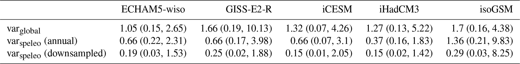
Variability of δ¹⁸O_iw is modeled differently in the simulations, as represented by the different levels of spectral power in the ratios. This difference is supported by the five area-weighted global variances of different magnitude and the simulated variance in annual and downsampled resolution as listed in Table 2. Small deviations between calculated variance and variance as area under the PSD can arise from the interpolation before the calculation of the spectra. The general order of isoGSM having the highest and iHadCM3 the lowest power on shorter frequencies remains throughout, as can also be seen in the table with small deviations to the order. The global variance, however, is only partly represented at the cave locations. While isoGSM shows the highest variance globally and at cave locations, iCESM is of medium variance globally but has the smallest variance at cave locations. For unweighted isotopic composition, the order of simulations changes (results not shown).

The analysis suggests that variability in the simulated δ¹⁸O_iw is represented differently in the simulations and that the order is not frequency dependent. The recorded δ¹⁸O_speleo shows more variability on centennial frequencies and less variability on decadal and smaller frequencies than the simulated values (albeit differing extents depending on the simulation).

Table 2 Area-weighted mean global δ¹⁸O_sim variances as var_global with 90 % intervals of the distribution are given per simulation. Row two and three give the δ¹⁸O_sim variance at the cave locations in the annual resolution of the simulation and downsampled to the records resolution, respectively.

4.4 Analysis of extreme events

To examine if there are factors that influence both δ¹⁸O_speleo and δ¹³C_speleo simultaneously, we analyze the similarity of both signals. A total of 86 % of the speleothems show significant correlation between both isotopes (results not shown). A different test for similarity is provided by checking for synchronous extreme events in the time series.

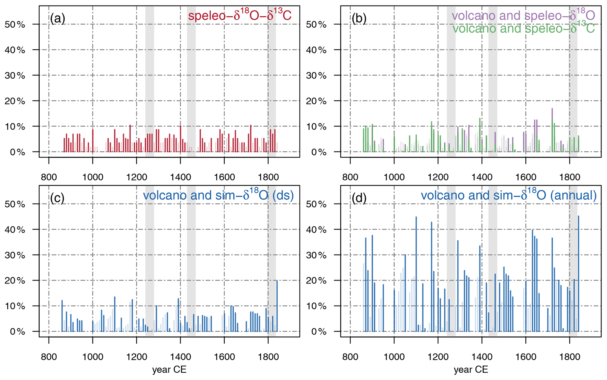
Figure 10 (a) The synchronous extreme events between δ¹⁸O_speleo and δ¹³C_speleo (red), (b) the synchronous events between the speleothem isotopes (oxygen purple and carbon green) and volcanic eruptions as reconstructed by Crowley and Unterman (2013) or Gao et al. (2008) (depicted in Fig. 1d), (c, d) the synchronous extreme events between simulated δ¹⁸O values at the cave locations of all simulations downsampled to record resolution and annual resolution, respectively. Where occurrence of synchronous extreme events is significant with α=0.05, the bars are shown in dark colors, where it is non-significant the bars are shown in transparent colors. The four light grey bars in the background of each plot show areas of high volcanic activity.

Figure 10 shows the temporal distribution of extreme events globally. In Fig. 10a we test for synchronous extreme events between the two isotopes by studying their relative timing to changes in volcanic forcing. Despite the high number of significantly correlated oxygen and carbon isotopes within one record, global patterns are not visible with a maximum of 10 % of speleothems showing synchronous extreme events between δ¹⁸O_speleo and δ¹³C_speleo at the same time over the last millennium. Synchronous events are also not higher in time periods of strong volcanic eruptions (indicated by grey bars).

By analyzing synchronous events between volcanic eruptions as reconstructed by Crowley and Unterman (2013) and Gao et al. (2008) (Fig. 1d) and δ¹⁸O_speleo as in Fig. 10b, up to 20 % of speleothems exhibit extreme events at the same time as extreme volcanic eruptions. This share is higher than for the carbon isotopes, where up to 15 % exhibit extreme events synchronous to volcanic eruptions. Both isotopes also show pronounced peaks occurring with different extreme volcano events (indicated by grey background) but also for minor volcanic events.

To check if the speleothems used here can resolve global extreme events of short duration, we compare δ¹⁸O_iw at the cave locations of each simulation to the volcanic forcing of the simulations (see Table 1). While up to 50 % of δ¹⁸O_iw at cave locations and annual resolution exhibit an extreme event at the same time as an extreme volcanic eruption (Fig. 10d), this number largely decreases to less than half when the resolution of δ¹⁸O_iw is decreased to that of the speleothems (Fig. 10c). The number of pseudo-speleothems experiencing synchronous events to volcanic forcing (Fig. 10c) is more similar to that of the speleothems (Fig. 10b). Summarizing, we see no global temporal pattern of synchronous extreme events in both δ¹⁸O_speleo and δ¹³C_speleo (Fig. 10a). A lower temporal resolution strongly decreases the ability of the modeled archive to resolve global events like volcanic eruptions.

5 Discussion

5.1 Comparison of oxygen isotope variability in isotope-enabled models and speleothems during the last millennium

We found that the mean δ¹⁸O_iw fields show global differences of up to 2.12 ‰ between the models that could most likely be attributed to the global mean temperature differences of up to 1.8 K between the models. Similarly, most of the strong regional differences in δ¹⁸O_iw between models could be explained by regional differences in simulated temperature (Fig. S5). This can be expected following the temperature effect (Dansgaard, 1964) or the more recently observed changes in isotopic signatures under the current anthropogenic warming trend (Rozanski et al., 1992). Temperature differences are, however, not the only explanation for differences in isotopic signatures between models, and individual model biases are also visible (Figs. S1 and S2). Specifically, we found less depletion of δ¹⁸O_iw in isoGSM over Antarctica as an artifact of its numerical scheme used for moisture transport and linked to extremely dry regions (Yoshimura et al., 2008). The warm bias in high latitudes for ECHAM5-wiso results is known to underestimate isotopic depletion (Werner et al., 2011, 2016). Overestimation of fractionation processes in iCESM during re-evaporation processes resulted in generally stronger depletion in δ¹⁸O_sim (Brady et al., 2019). The cool bias in northern mid-latitudes in the GISS-E2-R model as found in Schmidt et al. (2014) resulted in more depleted δ¹⁸O_iw in this region. Colder temperatures over Antarctica in iHadCM3 explained partly why isotopic signatures are a lot more depleted than in the other simulations. The iHadCM3 data, however, compares well to historical ice core data (Tindall et al., 2009), suggesting that the colder Antarctic conditions modeled by iHadCM3 may be more consistent with reality than the multi-model mean. Even though this study mostly focused on a terrestrial mid-to-low-latitude archive, local differences of modeled isotopic signatures in the Antarctic may have an influence on isotopic representation in the general circulation of the models.

At the cave locations, the spread between the simulations yielded 4.51 ‰ (90 % CI: 3.96, 4.79) in median (Fig. 3), while the median disagreement between simulated and speleothem δ¹⁸O_dweq was around −0.38 ‰ (−0.8, −0.23) (Fig. 4). This means that even though the simulations differed strongly in some regions, using multiple models can be sufficient to average out the disagreement at individual cave locations. The differences with the speleothems are in agreement with those found by Bühler et al. (2021), who compared the SISALv2 database to the iHadCM3 last millennium simulation. Median differences to the speleothem records were small for all models, where differences spatially around the globe (Fig. 3) reflected both the internal variability of models and global differences between the models. For example, ECHAM5-wiso showed the highest values for δ¹⁸O_iw in the global mean and also a more positive distribution than the other models. Differences in global mean δ¹⁸O_iw may arise from the weighting by the simulated evaporation and precipitation amounts, and while evaporation in ECHAM5-wiso is similar to the other models (Fig. S6), precipitation amounts are lower (Fig. S7). The lower oceanic precipitation amount can most likely be attributed to the coarser vertical resolution of ECHAM5-wiso (Hagemann et al., 2006).

Our analysis suggests that a multi-model approach is advisable whenever one is comparing mean modeled values to measured data. Even though global mean δ¹⁸O_iw values may be comparable, local and regional temperature estimates, and therefore modeled δ¹⁸O_iw values, can vary strongly and deviate between models. Even though isoGSM displayed the lowest disagreement between δ¹⁸O_iw and δ¹⁸O_speleo (Fig. 4), additional processes between meteoric water above the cave and drip water may again influence this difference. The multi-model offset comparison justified the use of the multi-model mean at cave locations in the following spatial analysis.

We found significant relationships between all considered modeled climatic variables (temperature, precipitation, and evaporation) and δ¹⁸O_iw with mean δ¹⁸O_dweq (Fig. 7). In general, the temperature and altitude effects on δ¹⁸O_speleo are visible in all latitude bands. Effects such as the precipitation amount relationship to δ¹⁸O_speleo are more distinct in the tropical and subtropical latitude band, which is in line with the effects described by Dansgaard (1964). In the extratropics, the precipitation effect is weak and overlapped by the altitude effect. We restricted our analysis to temperature, precipitation, and evaporation as they were available for all models. Future analyses that include more model diagnostics across the multi-model ensemble may find relationships to different variables that will improve our understanding of model biases and obtain a more coherent picture of which variables drive δ¹⁸O in the model world. The relationships between speleothem mean δ¹³C_c and meteorological variables from model ensemble mean (Fig. 8) were less clear, which again points to a more local influence.

Global studies that have evaluated δ¹⁸O_speleo isotopic signatures using climate models already exist (Bühler et al., 2021; Comas-Bru et al., 2019; Midhun et al., 2021), where regions with shared climatic features showed stronger relationships. For example, Baker et al. (2019) focused on specific climate zones by comparing drip water measurements to precipitation δ¹⁸O measurements and was able to identify temperature zones for which mean measured δ¹⁸O or δ¹⁸O_iw was most similar to δ¹⁸O_speleo. In our study, we found stronger relationships to climate variables in the individual latitude bands than on a global scale as in Bühler et al. (2021). Analyzing regions with high data density and similar climate patterns, we found even stronger temperature relationships (Figs. S8 and S9). Still, local particularities, such as large elevation differences over short distances, could not be resolved properly by the simulations and explained many of the stronger outliers, especially in the tropics.

Comparing a last century subset of the SISALv1 database by Fohlmeister et al. (2020) with our last millennium SISALv2 subset yielded similar results for precipitation and altitude relationships to δ¹³C_speleo (Fig. S10). In contrast to our latitudinal approach, they compared δ¹³C_speleo to temperature on a global scale. They neglected clusters of speleothems where factors other than temperature play an important role for the carbon isotope composition (e.g., high amounts of precipitation, known cave-specific particularities and processes, or temperatures close to the natural limit of vegetation, i.e., <5 ^∘C). The remaining records with temperatures between ∼7 to 27 ^∘C showed a positive trend between δ¹³C_speleo and temperature. This trend is in contrast to our observation based on clustering the records according to latitudinal bands. With this approach, we find no relationship between δ¹³C_speleo and temperature for the tropics and subtropics, but a clear inverse relationship between modeled temperatures and δ¹³C_speleo is observed for the extratropical records.

Higher cave site elevation coincided significantly with more depleted δ¹⁸O_dweq, which is in line with the altitude effect (Dansgaard, 1964). For δ¹³C_speleo, local studies exist that predict an increase in δ¹³C_speleo with higher altitude (Johnston et al., 2013). However, for the global last millennium subset of the SISALv2 database, more entities with carbon measurements in higher altitudes are needed to see a potential global relationship in addition to the relationship we find in the extratropical latitude bands.

5.2 Can models reproduce variability archived in speleothems?

For all simulations, temperature variability was the dominant driver in δ¹⁸O_iw at high latitudes and precipitation variability was dominant at low latitudes and in parts of the Antarctic (Figs. 5c and S5). However, local and regional climate dynamics, such as landward moisture transport and ice sheet changes, can mask and alter these relationships, as found for simulated isotopes in GISS-E2-R in a global study by LeGrande and Schmidt (2009). At the cave sites, model-internal regional variability and record age uncertainties substantially decreased correlation estimates. We observed that the sign of the correlation estimated between simulated temperature and δ¹⁸O_iw agreed at 60 % of cave locations for ≥3 simulations, and at 26 % for ≥4 simulations. For correlation estimates of precipitation, this was true only at 11 % or 1 % of locations, respectively. When compared to measured δ¹⁸O_speleo, we found more significant temporal correlation estimates to modeled temperature than to modeled precipitation (Fig. 5). This could in part be explained by global temperature responses to, e.g., volcanic forcing being more uniform between model ensemble runs compared to precipitation responses, which depend strongly on regional particularities. Regions with high inter-model climate variable spread (Fig. S11) also coincided with regions of the fewest significant correlation estimates to simulated temperature and the least agreement between the climatic drivers of δ¹⁸O_sim.

For variability specifically at the cave site locations, δ¹³C_speleo appeared to be more variable than δ¹⁸O_speleo on average on all timescales (Fig. 9d) with an increasingly higher variability compared to δ¹⁸O_speleo towards centennial timescales and longer (Fig. 9a). Within 86 % of all speleothems where both isotopes are provided, δ¹⁸O_speleo and δ¹³C_speleo showed significant correlations. Jointly explained variance in the isotopic signal can point towards common climatic drivers. However, the amplified variance on long timescales in δ¹³C_speleo could either hint at changes in the water cycle but also in land surface processes such as soil formation or vegetation composition and density. Considering more terrestrial archives and trace elements stored within the speleothems may help to better disentangle the climatic and environmental signals. On decadal and shorter timescales, where the meteoric and seasonal vegetation isotopic signal is mostly smoothed by the karst system, higher variability in δ¹³C_speleo may result from the stronger isotopic fractionation for carbon compared to oxygen in precipitated calcite (Polag et al., 2010; Hansen et al., 2019).

Climate models reflected δ¹⁸O_iw variability at cave locations to different extents. A clear offset between the models could be found on all timescales. We found no relationship between spatial resolution of the model and the variability of isotopic composition of precipitation. The higher-resolution run of iCESM and the lower-resolution run of iHadCM3 seem to show similar variability globally, and the lower-resolution ECHAM5-wiso shows even higher variability at the cave locations. Due to the strong impact of temperature and precipitation on δ¹⁸O_sim variability, we expect that this difference in isotopic variability also stems from the difference in the simulated climate. Further assessments using multivariate statistics are needed to firmly attribute the impact of climate on recorded variability of δ¹⁸O.

The lower temporal resolution of speleothem records largely explained the model–data mismatch on decadal and shorter timescales. Slow growth rates and limited sampling resolution lead to averaging effects that in turn lead to lower variability on decadal and shorter timescales. Simple karst-filters of a realistic transit time of ∼2.5 years (as in Fig. S12 and used in Bühler et al., 2021; Midhun et al., 2021; Dee et al., 2015) showed that variations in models and speleothems on these shorter timescales are similar if accounted for. Expert knowledge of the local cave hydrology is, however, needed for a more detailed assessment on which model reflects δ¹⁸O_iw variability best on decadal and shorter timescales compared to speleothems and may still be restricted by karst and cave internal processes that effectively limit the sampling of climatic signals.

On decadal and longer timescales, models seemed to underestimate δ¹⁸O_speleo variability, although to different extents, with isoGSM showing the highest variability and the smallest model–data mismatch. The model–data mismatch that we observed between speleothems and δ¹⁸O_iw starting at decadal timescales is in agreement with previous studies such as Laepple and Huybers (2014b). However, it is worth mentioning that speleothems may also be capable of enhancing climate-driven changes of δ¹⁸O and δ¹³C by cave-specific processes, resulting in higher variability on decadal and longer timescales. Under the assumption that variability on decadal and longer timescales is recorded correctly by speleothems, the iCESM model showed the strongest variability mismatch and isoGSM the smallest.

Cave locations were not necessarily reflective of mean annual δ¹⁸O variability globally – at least not in the model simulations. Simulations that showed generally high variability at cave locations at speleothem resolution also tended to be more variable globally and vice versa for low variability. However, simulations that were less variable at cave locations than others can still be more variable globally. In our case, this trend could likely be attributed to the bias of geographic locations of the cave sites as the models mostly show high variance in δ¹⁸O_iw in very dry regions and around the regions influenced by the Intertropical Convergence Zone.

5.3 Can external forcings be resolved by speleothems?

We found that 86 % of speleothems show a significant temporal correlation between speleothem oxygen and carbon isotopes, with 47 % even showing strong significant (anti-) correlations of $\left|c\right|>\mathrm{0.5}$. High co-variability between both isotopes can either be caused by kinetic fractionation processes (Hendy, 1971) in the cave environment or may be externally forced. For example, Fohlmeister et al. (2017) studied a stalagmite in an arid region and found strong correlation between the isotopes. They attribute increased correlation to times of strong variations in cave-internal processes triggered by variations of external conditions. This simultaneity agrees with our findings that generally no extreme event in isotopes precedes the other, which can, however, also be attributed to low sampling resolution. More local cave monitoring studies are necessary to potentially exclude kinetic fractionation effects as the dominant driver.

Temporal coherence between model and data can only be expected in the frequency space. However, variability associated with external forcing, such as volcanic eruptions or changes in solar forcing, may be imprinted in both model and data in a congruent time history (PAGESHydro2k-Consortium, 2017). Changes in temperature or precipitation due to aerosol-forced cooling have been analyzed in a δ¹³C record as signs of volcanic signatures of speleothems (Ridley et al., 2015). Growth rate changes (Baker et al., 1995) or the measurement of trace elements such as sulfur (Frisia et al., 2008) are other techniques to detect volcanic signals in speleothems, but they generally require up to sub-annual resolution records. In our global analysis of 58 δ¹³C_speleo and 89 δ¹⁸O_speleo records, we saw no significant increase in extreme events in the isotope records coinciding with major volcanic eruptions. The individual isotopes yielded more distinct signatures of volcanic eruptions, with up to 20 % (15 %) of speleothems recording synchronous extreme events in δ¹⁸O_speleo (δ¹³C_speleo) and a volcanic eruption, similar to δ¹⁸O_iw at record resolution. However, both stayed well below the possible simulated detection at cave locations under annual resolution of up to 50 %. The comparison to the synchronous events to the downsampled δ¹⁸O_iw showed that the ability to capture events such as volcanic eruptions strongly decreases with record resolution. The attribution of specific peaks in speleothem data to volcanic events needs caution because of age uncertainties and other possible explanations for the changes, e.g., human settlements close by (Baker et al., 1995). Increasing the bin size to the average age uncertainty within the last millennium subset of the SISALv2 yielded the same results (Fig. S13).

Solar variations are another external forcing that is often invoked as an influence on the monsoon cycle and has been investigated using speleothem records (Neff et al., 2001; Lone et al., 2014; Cosford et al., 2008). In these studies, it is also standard to use high-resolution speleothems with a lowest resolution of about 5 years for Lone et al. (2014). We repeated the analysis for Fig. 10 to analyze synchronous extreme events of δ¹⁸O_speleo and δ¹³C_speleo to the total solar irradiance input (Fig. S14). While the general effects of decreased detectability with decreased resolution are also visible, the overall detection of extreme solar irradiance was much weaker than for volcanic eruptions. This was not only true at cave locations but globally when comparing simulated surface climate variables to solar variations (results not shown). As solar variation on this timescale is mostly cyclical compared to random extreme volcanic eruptions (compare Fig. 1), these results were to be expected from the methods used and are not in contradiction to the literature.

The impact of different climatic backgrounds on the δ¹⁸O signal in speleothem records or paleoclimate simulations in time periods such as the Last Glacial Maximum and the Holocene have been studied extensively (e.g., Comas-Bru et al., 2019; Tierney et al., 2020; Parker et al., 2021). Periods of documented warmer and colder periods within the last millennium are for example the Little Ice Age (1550–1850 CE) or the Medieval Climate Anomaly (850–1250 CE) (definitions from Jones et al., 2001). We note that neither the global mean surface temperature nor the simulated δ¹⁸O or global δ¹⁸O as recorded by the speleothems showed significant changes to the mean state on a global scale within the described periods within the last millennium (results not shown). This is in line with Neukom et al. (2019), who found no global coherence of cold or warm periods over the Common Era, even though local changes are observable (e.g., McDermott et al., 2001).

Summarizing, the comparison to modeled valued showed that cave locations in this study are in general suitable to detect δ¹⁸O_iw variations due to modeled climatic changes in response to changes in volcanic or solar forcing. Even though speleothems are highly resolved archives with small age uncertainties compared to other archives, the median resolution during the last millennium of 6.08 years (4.07, 7.85) was not enough to resolve changes in δ¹³C_speleo or δ¹⁸O_speleo due to potential solar or volcanically induced climatic changes. Karst mixing effects which dampen the signal may decrease the ability to detect these changes even further.

5.4 Limitations

A current weakness of this type of analysis is that we only compared δ¹⁸O_sim of PMIP version 3 generation models to archived isotopes. However, parameter and tuning choices within one model, especially in the cloud and convection scheme, have a strong imprint on δ¹⁸O_sim signatures (for example Nusbaumer et al., 2017 for iCESM, Field et al., 2014 for GISS-E2-R). To further systematically explore and constrain modeled δ¹⁸O, a multi-model ensemble under different model setups will be needed. The multi-model comparison in this study only included how different models represent the oxygen isotopes, as δ¹³C is not included in isotope-enabled models yet. For iCESM, a carbon cycle in the ocean exists (Jahn et al., 2015), and great effort is put into the incorporation of a carbon cycle to isotope-enabled GCMs by the scientific community. However, this incorporation into GCMs cannot resolve the cave carbon cycle. Proxy system models of intermediate complexity that explicitly model soil carbon isotopes processes, temperature, moisture, and vegetation above the cave can be a more useful approach.

We also only looked at δ¹⁸O and δ¹³C as possible proxies for climatic changes. In contrast to, e.g., ice cores, speleothems do not directly record precipitation δ¹⁸O. Instead, both δ¹⁸O_speleo and δ¹³C_speleo undergo fractionation processes that are influenced by various cave-internal processes that may not be climate related (Lachniet, 2009; Fairchild and Baker, 2012; Hartmann and Baker, 2017; Dreybrodt and Scholz, 2011). Considering additional processes such as prior calcite precipitation (PCP) or other geochemical climate-related proxies can help to decipher the climatic signal from karst- or cave-internal processes (Kaufmann, 2003; Schwarcz et al., 1976; Owen et al., 2016; Tremaine and Froelich, 2013; Noronha et al., 2014).

When comparing the speleothem isotopes to volcanic data, we note that there now are more recent volcanic reconstructions available that suggest a modification to the timing or magnitude of last millennium eruptions (Sigl et al., 2015). Given the temporal resolution of the speleothems, changes in timing of volcanic events would impact the comparisons of model data to only those speleothems with high temporal resolution. As only the timing of the extreme event is compared, a change in magnitude would be irrelevant. As for the comparison with the simulated data, only the response of the model to any given eruption is important (Colose et al., 2016b), as we did not compare the timing of extreme events in speleothems to those in the simulation.

Compared to the capability of speleothems to cover complete glacial–interglacial cycles, we instead looked at short timescales when focusing on the last millennium and what drives variability on decadal to centennial timescales. The last millennium is considered a relatively stable time period, and climatic changes might not be strong enough to be fully captured by speleothems. On longer timescales, speleothems may still be a good archive to capture these larger changes (Genty et al., 2006).

6 Conclusion

We presented a multi-model comparison over five last millennium isotope-enabled simulations (ECHAM5-wiso, GISS-E2-R, iCESM, iHadCM3, and isoGSM) and compared their representation of isotopic signatures in mean and variability to paleoclimate data from a large speleothem database (a last millennium subset of SISALv2). We found that δ¹⁸O_iw differed substantially between models on a regional scale and at speleothem cave sites. This could in part be attributed to differences in simulated temperature, model biases in implementing SWI or topography, and cave- and site-specific controls on speleothem isotopes. Extreme model values that differ greatly from the rest can be compensated for by using the multi-model mean and thus reducing local spatial biases. The isoGSM simulation showed the lowest absolute mean difference to the speleothems at cave locations, while all other simulations show only slightly higher disagreements. Variability on decadal and longer timescales in the speleothems was higher than indicated by models and was also best represented by isoGSM; however, isoGSM still underestimated variability on these timescales. No relationship was found between the spatial resolution of the models and the variability of the isotopic composition of precipitation. In all models, temperature was driving δ¹⁸O_iw variability at high latitudes and precipitation at low latitudes. At cave site locations in particular, which are mostly located at low latitudes to mid-latitudes, models agreed more on temperature (rather than precipitation) being the driving factor of SWI variability. However, temperature signatures in climate models are generally more uniform than those of precipitation, as these depend heavily on how models parameterize convection and cloud dynamics (PAGESHydro2k-Consortium, 2017).

Dividing the global set into latitude bands, we were able to distinguish temperature and altitude relationships for both the oxygen and the carbon isotopes, as well as significant relationships for δ¹⁸O_dweq to other simulated climate variables. While most records showed significant correlation between the two isotopes, using both isotopes to gain more information than just from one remained difficult. This is especially difficult for variations in solar and volcanic forcing as they are not imprinted in either the single isotope or in the pair on a global scale. Many archive limitations could, however, be attributed to the low resolution of the dataset compared to the processes expected to be resolved.

This joint intercomparison of stable water isotopologue variability in both models and speleothem data is the first dataset in a time period of natural forcing and allows for further future analysis by the scientific community. Our analysis encourages the use of multi-model means whenever possible, as already suggested by other studies (Colose et al., 2016a). From the point of model evaluation, the incorporation of different archives with higher resolution (e.g., corals, trees, ice cores as in the Iso2k database; Konecky et al., 2020) and with the help of improved proxy system models may provide further insight into why offsets between models can be so large regionally. From a speleothem perspective, within-cave and between-cave variability comparisons using both isotopes will help us to understand the recorded signal better and give higher confidence in the results. Future multi-model comparisons of isotope-enabled models for other time periods are required to further evaluate biases in models, and comparisons to δ¹⁸O archives of all kinds are required to gain a deeper understanding of the underlying concept as to what influences variability and co-variability of isotopes in speleothems.