Comprehensive uncertainty estimation of the timing of Greenland warmings in the Greenland ice core records

Paleoclimate proxy records have non-negligible uncertainties that arise from both the proxy measurement and the dating processes. Knowledge of the dating uncertainties is important for a rigorous propagation to further analyses, for example, for identification and dating of stadial–interstadial transitions in Greenland ice core records during glacial intervals, for comparing the variability in different proxy archives, and for model-data comparisons in general. In this study we develop a statistical framework to quantify and propagate dating uncertainties in layer counted proxy archives using the example of the Greenland Ice Core Chronology 2005 (GICC05). We express the number of layers per depth interval as the sum of a structured component that represents both underlying physical processes and biases in layer counting, described by a regression model, and a noise component that represents the fluctuations of the underlying physical processes, as well as unbiased counting errors. The joint dating uncertainties for all depths can then be described by a multivariate Gaussian process from which the chronology (such as the GICC05) can be sampled. We show how the effect of a potential counting bias can be incorporated in our framework. Furthermore we present refined estimates of the occurrence times of Dansgaard–Oeschger events evidenced in Greenland ice cores together with a complete uncertainty quantification of these timings.

1 Introduction

The study of past climates is based on proxy measurements obtained from natural climate archives such as cave speleothems, lake and ocean sediments, and ice cores. Paleoclimate reconstructions derived from proxies suffer from 3-fold uncertainty. First, the proxy measurement itself involves the typical measurement uncertainties. Second, the interpretation of proxy variables, such as isotope ratios in terms of physical variables, such as temperature, is often ambiguous, and typically no one-to-one mapping can be established between the measured proxies and the climatic quantities of interest. Third, the age has to be measured alongside the proxy variable. In most cases an age model can be inferred that provides a quantitative relationship between the depth in the archive under consideration and the corresponding age. Such age models are also subject to uncertainties.

This study is exclusively concerned with the dating uncertainties of so-called layer counted archives, where the dating is performed based on counting periodic signals in the proxy archives such as annual layers arising from the impact of the seasonal cycle on the deposition process (e.g., Rasmussen et al., 2006). This type of archive comprises varved lake sediments, ice cores, banded corals, tree rings, and some speleothems (Comboul et al., 2014). Using the example of the NGRIP ice core (North Greenland Ice Core Project members, 2004) and its associated chronology, the GICC05 (Vinther et al., 2006; Rasmussen et al., 2006; Andersen et al., 2006; Svensson et al., 2008), we present here a statistical approach to generate ensembles of age models that may in turn be used to propagate the age uncertainties to any subsequent analysis of the time series derived from the NGRIP record. Our method can be directly adapted to other layer counted archives.

Layer counting assesses the age increments along the axis perpendicular to the layering, whose summation yields the total age. In turn, also the errors made in the counting process accumulate such that in chronologies obtained from counting annual layers, the absolute age uncertainty grows with increasing age (e.g., Boers et al., 2017).

Most importantly, dating uncertainties make it challenging to establish an unambiguous temporal relation between signals recorded in different, and possibly remote, archives. Therefore, it is often not possible to decipher the exact temporal order of events and distinguish causes from consequences across past climate changes. For example, abrupt Greenland warmings known as Dansgaard–Oeschger (DO) events (Dansgaard et al., 1993; Johnsen et al., 1992) evidenced in ice core records from the last glacial are accompanied by changes in the east Asian monsoon system, which are apparent from Chinese speleothem records (e.g., Zhou et al., 2014; Li et al., 2017). However, since the dating uncertainties exceed the relevant time scales of these abrupt climate shifts, a clear order of events cannot be determined. This prevents us from deducing if in the context of DO events, the abrupt Greenland warming triggered a hemispheric transition in the atmosphere, or vice versa, or if these changes happened simultaneously as part of a global abrupt climatic shift (Corrick et al., 2020).

For the quantification of dating uncertainties in radiometrically dated archives, there exist well established generalized frameworks. One example is the Bayesian Accumulation Model (Blaauw and Christeny, 2011) which models the sediment accumulation rate as a first order autoregressive process with gamma distributed innovations. Other methods or software include OxCal (Ramsey, 1995, 2008) and BChron (Haslett and Parnell, 2008; Parnell et al., 2008). Contrarily, the uncertainties of layer counted archives are targeted systematically only by few studies. Comboul et al. (2014) present a probabilistic model, where the number of missed and double-counted layers are expressed as counting processes shaped by corresponding error rates. However, this approach requires knowledge about these rates and further does not account for any uncertainty associated with them. An alternative Bayesian approach for quantifying the dating uncertainty of layer counted archives is presented in Boers et al. (2017), where the uncertainty is shifted from the time axis to the proxy value. However, this approach does not allow for generation of ensembles of chronologies as required for uncertainty propagation.

Even though dating uncertainties are conveniently quantified for many archives, many studies ignore these uncertainties and instead draw inference from “average” or “most likely” age scales, as already highlighted by McKay et al. (2021). This involves the risk of losing valuable information, as shown, for example, in Riechers and Boers (2020). In some cases, rigorous propagation of uncertainty may yield results that qualitatively differ from results obtained by using the “average” or “best fit” age model. In this context, McKay et al. (2021) propose to apply the respective analysis to an ensemble of possible age scales to ensure the uncertainty propagation, in line with the strategy proposed by Riechers and Boers (2020).

We focus on the layer counted part of the GICC05 chronology, a synchronized age scale for several Greenland ice cores (Vinther et al., 2006; Rasmussen et al., 2006; Andersen et al., 2006; Svensson et al., 2008). It was obtained by counting the layers of different Greenland ice cores and synchronizing the results using matchpoints. While the recent part of the chronology is compiled from multiple cores, the older part (older than 15 kyr b2k) is based exclusively on the layer counting in the NGRIP core. We introduce a new method to generate realistic age ensembles for the NGRIP core, which conveniently represent the uncertainty associated with the GICC05.

Originally, the dating uncertainty of the GICC05 is quantified in terms of the maximum counting error (MCE). The MCE increases by 0.5 years for every layer which is deemed uncertain by the investigators during the counting process:

$$\begin{array}{}\text{(1)}& \mathrm{MCE}\left(z\right)=\mathrm{0.5}{N}_{\mathrm{u}}\left(z\right),\end{array}$$

where N_u is the number of uncertain layers down to depth z. In contrast to certain layers, which can be identified unambiguously in the records, uncertain layers are less pronounced and therefore it seems less certain that these signals truly correspond to physical layers. The accumulation of uncertain layers results in high values for the MCE for the older parts of the core (MCE =2.6 kyr at 60 kyr b2k estimated age). However, it seems highly unlikely that all uncertain layers are consistently either true layers or no layers, which is why we think that the MCE is an overly careful quantification of the age uncertainty, as already suggested by Andersen et al. (2006). One might, alternatively, be tempted to treat the uncertain layers as a Bernoulli experiment with N_u repetitions and a probability of one half for each uncertain layer to be a true layer. However, this would neglect any sort of bias in the assessment of the uncertain layers and would lead to unrealistically small uncertainties, since over- and undercounting practically cancel each other out in this Bernoulli type interpretation (see for instance Andersen et al., 2006; Rasmussen et al., 2006).

The method presented here abandons the notion of certain and uncertain layers. Instead, we separate the GICC05 chronology into contributions that can be captured by deterministic model equations and corresponding residuals. We construct a new age–depth model by complementing the deterministic part with a stochastic component designed in accordance with the statistics of the residuals. This model can be used to generate age–depth ensembles in a computationally efficient manner. In turn, these ensembles facilitate uncertainty propagation to subsequent analysis. The model parameters are tuned with respect to the GICC05 chronology that includes every uncertain layer as half a layer.

The outline of this paper is as follows: Section 2 gives a description of the data used for this study. Section 3.1 introduces our statistical model for the dating uncertainties, and details about how we incorporate physical processes and how we deduce the noise of the model from the statistics of the residuals. In Sect. 3.2 we show how we can formulate our model in terms of a hierarchical Bayesian modeling framework that allows for the physical and noise components to be estimated simultaneously. That section also details how one can use the resulting posterior distributions of the model parameters to obtain a full description of the posterior distributions of the dating uncertainties using a sample-based approach. We finally demonstrate how a potential counting bias could be incorporated by the model, and how that would affect the results. In Sect. 4 we show how our model can be used to obtain a full description of the dating uncertainties of abrupt warming events, which takes into account the dating uncertainties as well as the uncertainties in determining their exact position in the noisy data. Further discussion and conclusions are provided in Sect. 6.

2 NGRIP ice core data

We use the Greenland Ice Core Chronology 2005 (GICC05) (Vinther et al., 2006; Rasmussen et al., 2006; Andersen et al., 2006; Svensson et al., 2008) as defined for the NGRIP ice core together with the corresponding δ¹⁸O proxy record (North Greenland Ice Core Project members, 2004; Gkinis et al., 2014; Ruth et al., 2003). An analogous analysis for the Ca²⁺ proxy record is presented in Appendix B. The final age of the layer counted part of the GICC05 is 59 944 yr b2k, and we consider data up to 11 703 yr b2k. The following Holocene part of the record is excluded since it is governed by a substantially different climate than the last glacial interval (Rasmussen et al., 2014). For the considered period, the NGRIP record is available at 5 cm resolution and thus equidistant in depth, but not in time. In total, the data comprises n=18 672 data points of the form $(z_k,y_k,x_k),k\in \mathit{\{}\mathrm{0},\mathrm{1},\mathrm{\dots },n-\mathrm{1}\mathit{\}}$, where z_k denotes the kth depth, y_k the corresponding age as indicated by the GICC05, and x_k the measured proxy value.

The GICC05 is based on counting annual layers which are evident in multi-proxy continuous flow measurements from the NGRIP, DYE3, and the GRIP ice cores. While the measurements from DYE3 and GRIP only facilitate layer counting up to ages of 8.2 and 14.9 kyr b2k, respectively, the NGRIP core allowed the identification of annual layers up to an age of 60 kyr b2k. The uncertainty of the GICC05 has been quantified as follows: whenever the investigators were uncertain about whether or not a signal in the data should be considered an annual layer, half a year was added to the cumulative number of layers while simultaneously adding ±0.5 yr to the age uncertainty. The total age uncertainty determined by the number of all uncertain layers up to a given depth is termed the maximum counting error (MCE). The MCE amounts to a relative age uncertainty of 0.84 % at the onset of the Holocene and 4.34 % at the end of the layer counted section of the core.

δ¹⁸O values from Greenland ice cores are interpreted as a qualitative measure of the site temperature at the time of precipitation (Jouzel et al., 1997; Gkinis et al., 2014). We include these data in our study since our modeling approach will make use of the relation between atmospheric temperatures and the amount of precipitation, which in turn affects the thickness of the annual layers. In addition we use the division of the record into Greenland stadial and interstadial phases as presented in Table 2 of Rasmussen et al. (2014). We label the depths at which stadial–interstadial transitions occur by $z_{\mathrm{1}}^{\ast },\mathrm{\dots },z_p^{\ast }$ and the corresponding ages by $y_{\mathrm{1}}^{\ast },\mathrm{\dots },y_p^{\ast }$. Figure 1 shows the measured δ¹⁸O values as a function of the GICC05 time scale, together with the Greenland stadial and interstadial onsets.

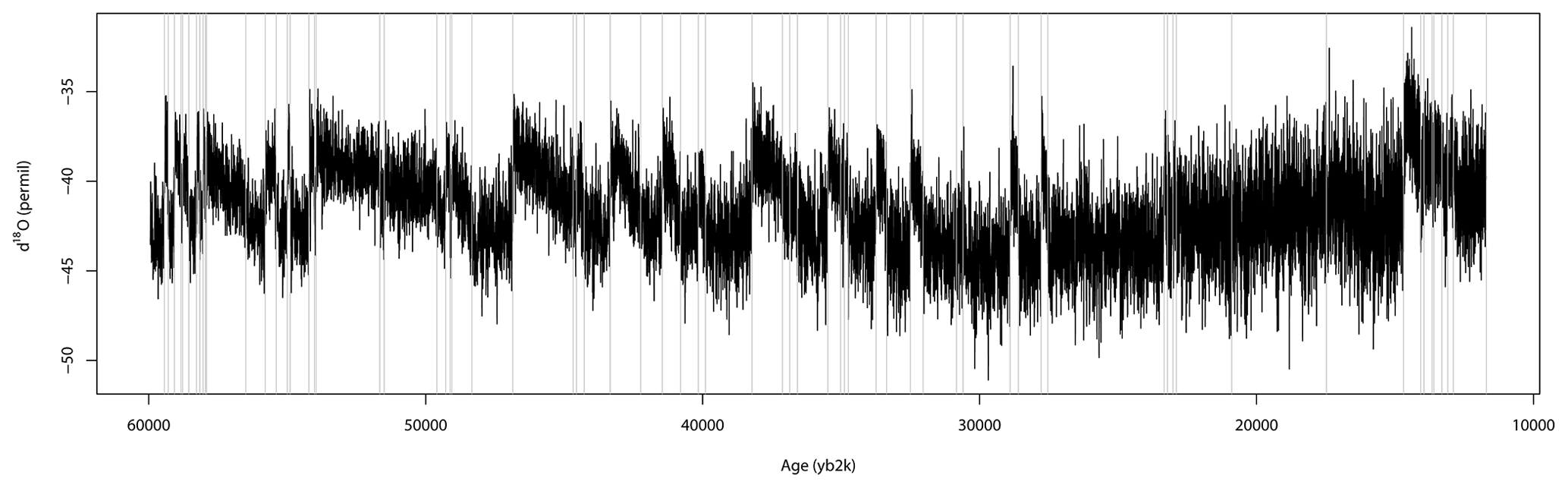
Figure 1 The measured δ¹⁸O isotope values plotted against the corresponding GICC05 time scale, starting from 11 793 yr b2k. The vertical gray lines denote the transitions between Greenland stadial and interstadial periods as reported by Rasmussen et al. (2014).

3 Methods

3.1 Age–depth model

We assume that depths $\mathit{z}=(z_{\mathrm{1}},\mathrm{\dots },z_n{)}^{\top }$ and proxy values $\mathit{x}=(x_{\mathrm{1}},\mathrm{\dots },x_n{)}^{\top }$ are measured accurately and hence treat them as deterministic variables. In contrast, we consider the ages $\mathit{y}=(y_{\mathrm{1}},\mathrm{\dots },y_n{)}^{\top }$ as dependent stochastic variables and will in the following establish a model to map the independent depths and stable isotope concentrations onto ages, in a way that reflects the uncertainties inherent to the dating. The model will be supplemented with information on the prevailing climate period.

In order to motivate our modeling approach we give some general considerations about the deposition process as well as the counting process. The decisive quantity for us will be the incremental number of annual layers counted in a 5 cm depth increment of the ice core:

$$\begin{array}{}\text{(2)}& \mathrm{\Delta }{y}_k=y_k-y_{k-\mathrm{1}}.\end{array}$$

This quantity is determined by the amount of precipitation (minus the snow that is blown away by winds) during the corresponding period, the thinning that the layers experience over time deeper down in the core, and potential errors made during the counting process. While the thinning process can be expected to happen mostly deterministically, the net annual accumulation of snow certainly exhibits stronger fluctuations. Finally, the counting error adds additional randomness. Thus, it is reasonable to regard the observed age increments Δy as a realization of a random vector ΔY which can be decomposed into a deterministic and a stochastic component:

$$\begin{array}{}\text{(3)}& \mathrm{\Delta }{Y}_k=a\left(z_k\right)+{\mathit{\epsilon }}_k.\end{array}$$

Note that the number of layers within a 5 cm depth increment is not necessarily an integer number. Given that the amount of precipitation co-varies with atmospheric site temperatures we can specify

$$\begin{array}{}\text{(4)}& a\left(z_k\right)=a\left(z_k,x\left(z_k\right)\right)\to a\left(z_k,x_k\right).\end{array}$$

Based on physical arguments and the analysis of the observed age increments Δy_k, we will propose the structural form of the deterministic part of the model and then tune the model parameters to the data. In turn, this will allow us to design the model's noise component ε in accordance with the corresponding residuals ${\mathit{\delta }}_k=\mathrm{\Delta }{y}_k-a\left(z_k,x_k\right)$.

3.1.1 Linear regression

As explained above, the thickness of the counted layers, and thereby the number of layers per depth increment $\mathrm{\Delta }{z}_k=z_k-z_{k-\mathrm{1}}$, is governed by two physical factors: the amount of precipitation at the time the layer was formed and the thinning of the core due to ice flow. These processes are here assumed to follow a regression model. We take into account the thinning by implementing a second order polynomial dependency of ΔY_k with respect to the depth z_k. Choosing this non-linear function conveniently accounts for the saturation of the layer thinning evident in the NGRIP ice core. The amount of precipitation is known to co-vary with atmospheric temperatures, since by the Clausius–Clapeyron relation the moisture holding capacity of the atmosphere increases with temperatures. This is represented using a linear response to the δ¹⁸O measurements. The same response is applied to the log(Ca²⁺) in the alternative analysis presented in Appendix B. Finally, we observe clear trends in the incremental layers that persist over individual stadials and interstadials. Given the consistency of these trends across the different climate periods, we decided to incorporate them into the deterministic model component. Overall, we propose a deterministic model of the form

$$\begin{array}{}\text{(5)}& a\left(z_k,x_k\right)=b{z}_k^{\mathrm{2}}+b_x{x}_k\left(z_k\right)+\sum _{i=\mathrm{1}}^p{\mathit{\psi }}_i(z_k;a_i,c_i),\end{array}$$

with

$$\begin{array}{}\text{(6)}& {\mathit{\psi }}_i\left(z_k;a_i,c_i\right)=\left\{\begin{array}{ll}{a}_i+c_i{z}_k,& z_i^{*}<z_k<z_{i+\mathrm{1}}^{\ast }\\ \mathrm{0},& \mathrm{otherwise}\end{array}\right.,\end{array}$$

in order to capture the systematic features of the chronology. Here, c_i denotes the period specific slopes and a_i their corresponding offsets. For p transitions between stadials and interstadials we have to tune 2p+2 regression parameters, which is achieved by fitting the above model for a(z_k,x_k) to the observed layer increments Δy_k given by the GICC05 time scale in a least squares approach. As explained above, the GICC05 ages contain the contribution of uncertain layers, which were counted as half a year each. Here, we abandon the distinction of certain and uncertain layers and regard the GICC05 ages as the best possible estimate of the true ages and accordingly use them directly for the optimization. The fitted model is shown in red in Fig. 22a.

3.1.2 Noise structure

After tuning the deterministic part of Eq. (3), the residuals are given by

$$\begin{array}{}\text{(7)}& {\mathit{\delta }}_k=a\left(z_k,x_k\right)-\mathrm{\Delta }{y}_k.\end{array}$$

We find the residuals to be symmetric and unimodally distributed, and apart from some degree of over-dispersion they appear to be well described by a normal distribution, as shown in Fig. 3.

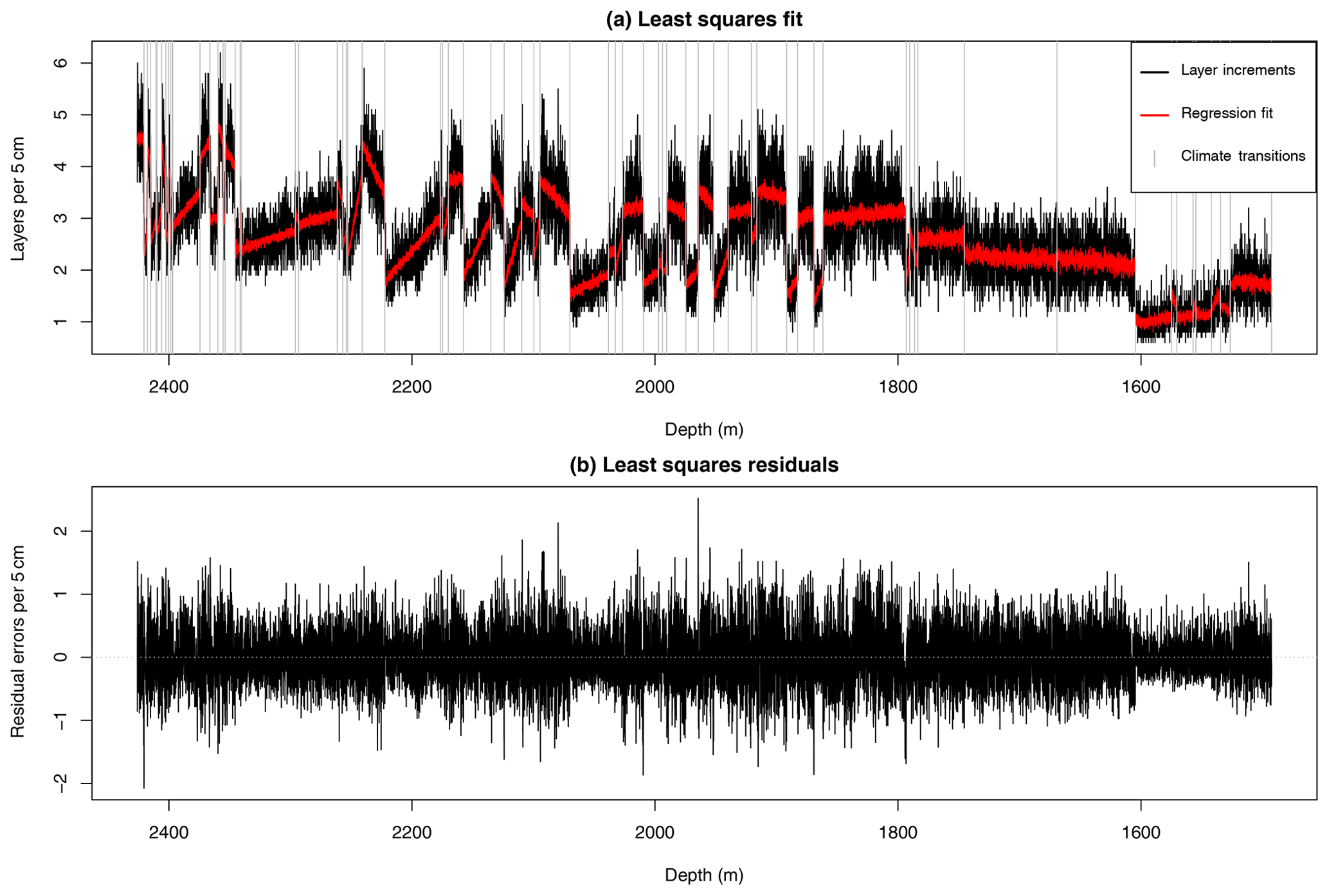
Figure 2 (a) Number of layers counted in the GICC05 time scale per 5 cm depth increments in the NGRIP ice core (black). The red line shows the fitted values from the regression model $a(z_k,x_k)=b{z}_k^{\mathrm{2}}+b_{x}x\left(k\right)+{\sum }_{i=\mathrm{1}}^p{\mathit{\psi }}_i(z_k;a_i,c_i)$. The vertical gray lines represent the transitions between Greenland stadials and interstadials. (b) The residuals δ_k obtained from fitting the regression model a(z_k,x_k) to the layer increments Δy_k.

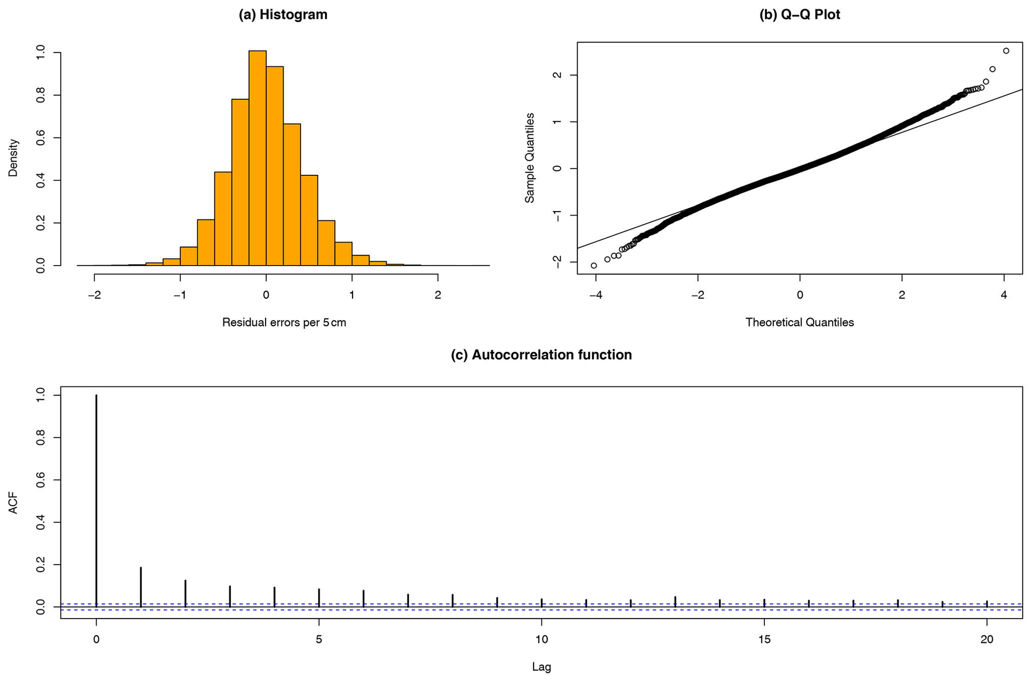
Figure 3 (a) Histogram of the residuals obtained from least squares fit of the regression model a(z_k,x_k). (b) The corresponding quantile–quantile plot. We observed key properties of symmetry and unimodality indicating Gaussianity. The quantile–quantile plot indicates a small over-dispersion, but overall the data seem to be consistent with a normal distribution. (c) The autocorrelation function of the residuals from the least squares fit of the linear regression model, up to a maximum of 20 lags. A fast memory decay can be inferred.

Moreover, by examining the empirical autocorrelation illustrated in Fig. 3c, we observe that the residuals exhibit a fast decay of memory which is indicative of stationarity. This suggests that the noise can be expressed using a short-memory Gaussian stochastic process.

We explore three different models for the correlation structure of the noise ε. The first model assumes that they follow independent and identically distributed (iid) Gaussian processes:

$$\begin{array}{}\text{(8)}& {\mathit{\epsilon }}_k\stackrel{\mathrm{iid}}{\sim }\mathcal{N}\left(\mathrm{0},{\mathit{\sigma }}_{\mathit{\epsilon }}^{\mathrm{2}}\right).\end{array}$$

The second model assumes that the noise can be described by a first order autoregressive (AR) process

$$\begin{array}{}\text{(9)}& {\mathit{\epsilon }}_k=\mathit{\varphi }{\mathit{\epsilon }}_{k-\mathrm{1}}+{\mathit{\xi }}_k,\end{array}$$

where ϕ is the first-lag autocorrelation coefficient and ξ_k is a white noise process with variance ${\mathit{\sigma }}_{\mathit{\xi }}^{\mathrm{2}}={\mathit{\sigma }}_{\mathit{\epsilon }}^{\mathrm{2}}/(\mathrm{1}-{\mathit{\varphi }}^{\mathrm{2}})$. The third model assumes the noise follows a second order autoregressive process

$$\begin{array}{}\text{(10)}& {\mathit{\epsilon }}_k={\mathit{\varphi }}_{\mathrm{1}}{\mathit{\epsilon }}_{k-\mathrm{1}}+{\mathit{\varphi }}_{\mathrm{2}}{\mathit{\epsilon }}_{k-\mathrm{2}}+{\mathit{\xi }}_k,\end{array}$$

where ϕ₁ and ϕ₂ are the first- and second-lag autocorrelation coefficients and ξ_k is a white noise process with variance:

$$\begin{array}{}\text{(11)}& {\mathit{\sigma }}_{\mathit{\xi }}^{\mathrm{2}}={\mathit{\sigma }}_{\mathit{\epsilon }}^{\mathrm{2}}{\displaystyle \frac{\mathrm{1}-{\mathit{\varphi }}_{\mathrm{2}}}{\left(\mathrm{1}+{\mathit{\varphi }}_{\mathrm{2}}\right)\left({\left(\mathrm{1}-{\mathit{\varphi }}_{\mathrm{2}}\right)}^{\mathrm{2}}-{\mathit{\varphi }}_{\mathrm{1}}^{\mathrm{2}}\right)}}.\end{array}$$

Note that a potential global or at least climate-regime-specific bias in the counting process, such as overseeing systematically 1 out of 10 layers, would be captured by the regression model and thus cannot be identified as a systematic error. We will investigate the influence of potential systematic errors below. Similarly, fluctuations in the physical processes can be captured by the noise model which aims to represent the counting errors. It would therefore be more accurate to interpret a(z_k,x_k) as a structured component representing a part of both the physical processes and a systematic counting error which can be accounted for by linear regression, and ε_k as the fluctuations of both the physical processes and counting errors. Hence, ε_k can be considered an upper boundary on the counting uncertainty.

3.2 Simultaneous Bayesian modeling

So far, we have fitted only the structural model component. This enabled us to investigate statistical properties of the residuals and formulate corresponding noise model candidates. Fitting both the linear regression model and the different noise models can in principle be performed in two stages: First, the linear regression model is fitted to the layer increments using the method of least squares. Thereafter, the fitted values are subtracted and the selected noise model is fitted to the residuals. However, this approach has the disadvantage that some variation that may in reality be caused by the noise process ε_k may have been attributed to the structured component a(z_k,x_k) and removed before fitting the noise model. We therefore introduce here a Bayesian approach that enables us to estimate all model parameters simultaneously. The Bayesian approach has three key advantages over the least squares fitting of the structured component: first, it treats the noise and the structured component equally. Second, it returns the joint posterior probability of all model parameters which indicates the plausibility of a certain parameter configuration in view of the data. The posterior probability distribution can be regarded as an uncertainty quantification of the model's parameter configuration. Third, in the Bayesian parameter estimation, prior knowledge and constraints on the parameter can be incorporated via a convenient choice of the so-called prior distributions.

In general terms, let 𝒟 denote some observational data and θ denote parameters that shape a model which is assumed to reasonably describe the process that generated the data. Then Bayes' theorem can be used to deduce the posterior probability density of the parameters θ given the data 𝒟:

$$\begin{array}{}\text{(12)}& \mathit{\pi }\left(\mathit{\theta }\right|\mathcal{D})={\displaystyle \frac{\mathit{\pi }\left(\mathcal{D}\right|\mathit{\theta }\left)\mathit{\pi }\right(\mathit{\theta })}{\mathit{\pi }\left(\mathcal{D}\right)}}.\end{array}$$

In our case the GICC05 age $\mathit{y}=(y_{\mathrm{1}},\mathrm{\dots },y_n)$, or more precisely their increments Δy, represent the observational data 𝒟 assumed to be generated from the model defined by Eq. (3). There are 2p+2 parameters $\mathit{\beta }=(b_{\mathrm{2}},b_x,a_{\mathrm{1}},c_{\mathrm{1}},\mathrm{\dots },a_p,c_p)$ for the structured component alone and the noise adds another one to three parameters, depending on the choice of the noise structure. Thus the set of model parameters reads

$$\begin{array}{}\text{(13)}& \mathit{\theta }=\left(\mathit{\beta },\mathit{\psi }\right),\end{array}$$

where ψ=σ_ε if the residuals are assumed to follow an iid Gaussian distribution, $\mathit{\psi }=({\mathit{\sigma }}_{\mathit{\epsilon }},\mathit{\varphi })$ if they are assumed to follow an AR(1) process, and $\mathit{\psi }=({\mathit{\sigma }}_{\mathit{\epsilon }},{\mathit{\varphi }}_{\mathrm{1}},{\mathit{\varphi }}_{\mathrm{2}})$ if they are assumed to follow an AR(2) process. For any given parameter configuration, the likelihood is for all three choices of the noise structure defined by a multivariate Gaussian distribution,

$$\begin{array}{}\text{(14)}& \begin{array}{rl}\mathit{\pi }\left(\mathrm{\Delta }\mathit{y}|\mathit{\theta }\right)& ={\left(\mathrm{2}\mathit{\pi }\right)}^{-n/\mathrm{2}}\left|\mathbf{\Sigma }\right|{}^{-\mathrm{1}}\exp \left\{-{\displaystyle \frac{\mathrm{1}}{\mathrm{2}}}\left(\mathrm{\Delta }\mathit{y}\right.\right.\\ & \left.{\left.-\mathit{a}\right)}^{\top }{\mathbf{\Sigma }}^{-\mathrm{1}}\left(\mathrm{\Delta }\mathit{y}-\mathit{a}\right)\right\},\end{array}\end{array}$$

where $\mathit{a}=\left(a\right(z_{\mathrm{1}},x_{\mathrm{1}}),\mathrm{\dots },a(z_n,x_n){)}^{\top }$ and the entries of the autocovariance matrix Σ are given by the autocovariance function ${\mathrm{\Sigma }}_{ij}=\mathit{\gamma }\left(\right|i-j\left|\right)$ of the assumed noise model. For the iid model, the autocovariance function is simply ${\mathit{\sigma }}_{\mathit{\epsilon }}^{\mathrm{2}}$ if i=j, and zero otherwise, resulting in a diagonal covariance matrix. For the AR(1) model the autocovariance function is

$$\begin{array}{}\text{(15)}& \mathit{\gamma }\left(k\right)={\displaystyle \frac{{\mathit{\sigma }}_{\mathit{\epsilon }}^{\mathrm{2}}}{\mathrm{1}-{\mathit{\varphi }}^{\mathrm{2}}}}{\mathit{\varphi }}^{\left|k\right|}.\end{array}$$

The autocovariance function of the AR(2) model is specified by the difference equation,

$$\begin{array}{}\text{(16)}& \mathit{\gamma }\left(k\right)={\mathit{\varphi }}_{\mathrm{1}}\mathit{\gamma }(k-\mathrm{1})+{\mathit{\varphi }}_{\mathrm{2}}\mathit{\gamma }(k-\mathrm{2}),\end{array}$$

with initial conditions:

$$\begin{array}{}\text{(17)}& {\displaystyle }\mathit{\gamma }\left(\mathrm{0}\right)& {\displaystyle }=\left({\displaystyle \frac{\mathrm{1}-{\mathit{\varphi }}_{\mathrm{2}}}{\mathrm{1}+{\mathit{\varphi }}_{\mathrm{2}}}}\right){\displaystyle \frac{{\mathit{\sigma }}_{\mathit{\epsilon }}^{\mathrm{2}}}{(\mathrm{1}-{\mathit{\varphi }}_{\mathrm{2}}{)}^{\mathrm{2}}-{\mathit{\varphi }}_{\mathrm{1}}^{\mathrm{2}}}}\text{(18)}& {\displaystyle }\mathit{\gamma }\left(\mathrm{1}\right)& {\displaystyle }={\displaystyle \frac{{\mathit{\varphi }}_{\mathrm{1}}}{\mathrm{1}-{\mathit{\varphi }}_{\mathrm{2}}}}\mathit{\gamma }\left(\mathrm{0}\right).\end{array}$$

A benefit of having the likelihood follow a Gaussian distribution is that it can be evaluated easily and samples can be obtained efficiently, despite the large number of parameters. Finally, we define convenient priors for the model parameters. For the parameters of the structured model component β we choose vague Gaussian priors, with variances that safely cover all reasonable parameter configurations. For the noise parameters ψ we restrict the scaling parameter σ_ε to be positive, and the autoregressive coefficients such that they define a stationary model. These constraints are embedded into the model by adopting suitable parameterizations. The scaling parameter σ_ε is assigned a gamma distribution through the parameterization $\mathit{\kappa }=\log (\mathrm{1}/{\mathit{\sigma }}_{\mathit{\epsilon }}^{\mathrm{2}})$. For the lag-one correlation parameter in the AR(1) model we assume a Gaussian prior on the logit transformation $\mathit{\rho }=\log \left(\right(\mathrm{1}+\mathit{\varphi })/(\mathrm{1}-\mathit{\varphi }\left)\right)$. For the AR(2) model we instead assign priors on the logit transformation of the partial autocorrelations ${\mathit{\psi }}_{\mathrm{1}}={\mathit{\varphi }}_{\mathrm{1}}/(\mathrm{1}-{\mathit{\varphi }}_{\mathrm{2}})$ and ψ₂=ϕ₂, using penalized complexity priors (Simpson et al., 2017).

In principle, the joint posterior density can then be sampled by using a Markov chain Monte Carlo (MCMC) algorithm (e.g., Goodman and Weare, 2010). However, to solve Eq. (12) more efficiently, we formulate the problem in terms of a latent Gaussian model and then use integrated nested Laplace approximations (INLAs) (Rue et al., 2009, 2017) to compute the joint and marginal posterior distributions (for details see Appendix A).

The posterior distribution of θ enables us to generate ensembles of different realizations of the random variable Y, i.e., of the age increments that correspond to the fixed depth increments Δz. In a two-stage Monte Carlo simulation, first a value for θ is randomly sampled from the posterior π(θ|Δy). Second, the noise ε is sampled according to the noise model using noise parameters sampled in the first step. An ensemble generated in this fashion simultaneously reflects the uncertainty enshrined in the stochastic process and the model thereof as well as the uncertainty about the model parameters. Each realization of age increments yields a corresponding possible chronology according to

$$\begin{array}{}\text{(19)}& y_k=y_{\mathrm{0}}+\sum _{i=\mathrm{1}}^k\left(a\left(z_i,x_i\right)+{\mathit{\epsilon }}_i\right),\end{array}$$

where y₀ is the number of reported layers up to the depth z₀. Figure 4 shows the 95 % credible intervals obtained from age ensembles for the three different noise models with respect to the GICC05 age. Each ensemble comprises 10 000 realizations of Y. In this plot we notice a significant increase of uncertainty going from the iid to the AR(1) model. This is intuitive as when more memory is added to the model, the variation increases.

However, going from AR(1) to AR(2) adds only moderate additional uncertainty. We therefore argue that an AR(1) process is sufficient in terms of modeling the correlation structure of the residuals. The same is observed when using log(Ca²⁺) as a proxy instead (see Fig. B1). All computations henceforth are carried out with the AR(1) noise model.

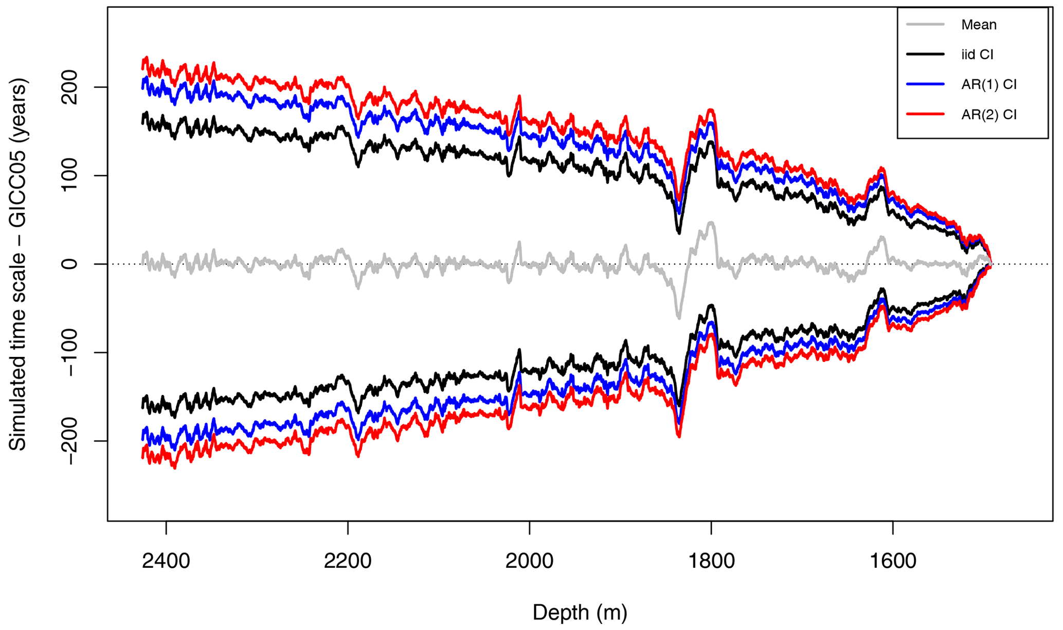
Figure 4 The 95 % credible intervals of the dating uncertainty distribution when δ¹⁸O is used as the proxy covariate. The GICC05 time scale has been subtracted and the noise is modeled using iid (black), AR(1) (blue), and AR(2) (red) noise models. Only the posterior marginal mean computed using AR(1) distributed noise is included (gray) since it is very similar to the mean obtained using other noise assumptions.

3.3 Incorporating an unknown counting bias

When originally quantifying the uncertainty of the GICC05 chronology, a concern was that the layer counting was potentially biased in the sense that layers were consistently over-counted or missed. As highlighted by Andersen et al. (2006), there is no way to quantify a potential bias based on the data. Here, we investigate the influence that such a bias would have on our model, assuming a given maximum bias strength. To capture the effect of a systematic bias in the layer counting we introduce a scaling parameter η such that

$$\begin{array}{}\text{(20)}& \mathrm{\Delta }{Y}_k=\mathit{\eta }\left(a\left(z_k,x_k\right)+{\mathit{\epsilon }}_k\right).\end{array}$$

Given that we have no knowledge about the size of the bias, η must be regarded as a random variable whose distribution can only be estimated by experts a priori. Originally, biases on the order of 1 % in the counting performed by different investigators have been observed (Rasmussen et al., 2006; Andersen et al., 2006). Here we assume

$$\begin{array}{}\text{(21)}& \mathit{\eta }\sim \mathcal{U}\left(\mathrm{1}\pm \mathrm{\Delta }\mathit{\eta }\right),\end{array}$$

meaning the layer counters are just as likely to systematically over-count as to under-count, on a maximum rate of Δη. While the expectation for the age increments E(ΔY) remains unchanged as long as E(η)=1, their variance will grow due to the additional uncertainty. Figure 5 shows the 95 % credible intervals for potentially biased chronology ensembles generated under the assumption that Δη equals 0 %, 2 %, or 4 %.

It is evident that the bias uncertainty contributes substantially to the age uncertainty. This is expected since a relatively small counting bias yields a large absolute error at a possible age of 60 kyr b2k, which in turn exceeds the uncertainty contribution of the noise by far. We also observed that one would need a maximum error rate of Δη≈4 % in order for the uncertainty to approach the maximum counting error at the end of the layer counted core segment.

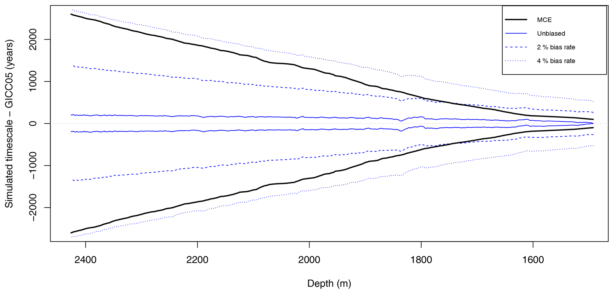
Figure 5 The 95 % credible intervals of the difference between estimated dating and the GICC05 time scale compared with the maximum counting error (solid black). Dating uncertainties in this case include a bias expressed by a stochastic scaling parameter drawn from a uniform 𝒰(1±Δη) distribution. The solid blue line represents the unbiased Δη=0 dating uncertainty, while the dashed and dotted blue lines represent the biased cases of Δη=2 % and Δη=4 %, respectively. The differences in dating uncertainty between iid, AR(1), and AR(2) models are dwarfed by the uncertainty introduced by the unknown bias; hence, only the AR(1) distributed residuals are shown here.

4 Examples of applications

4.1 Dating uncertainty of DO events

Both the NGRIP δ¹⁸O and log(Ca²⁺) records are characterized by prominent abrupt shifts from low to high values, including the so-called Dansgaard–Oeschger (DO) events (Johnsen et al., 1992; Dansgaard et al., 1993). These jumps are interpreted as sudden warming events in Greenland, which took place repeatedly during the last glacial period. In order to explain the physical relationship between these abrupt Greenland warming events and apparently concomitant abrupt climate shifts evidenced in other archives from different parts of the planet, it is crucial to disentangle the exact temporal order of these events. This requires a rigorous treatment of the uncertainties associated with the dating of DO events in Greenland ice core records.

Rasmussen et al. (2014) provide a comprehensive list of Dansgaard–Oeschger events and other stadial–interstadial transitions, indicating depths from the NGRIP ice core at which they occur, and the corresponding GICC05 age. They report the visually identified event onsets and provide uncertainty estimates in terms of data points along the depth axis and the respective MCE associated with the estimated event onset depth. This assessment was later refined by Capron et al. (2021) using the algorithm for detecting transition onsets designed by Erhardt et al. (2019). Here, we present a rigorous combination of the depth and age uncertainties, which complicate the exact dating of abrupt warming events.

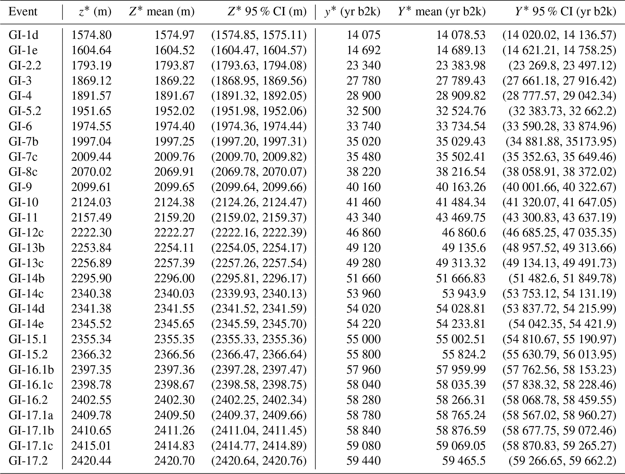
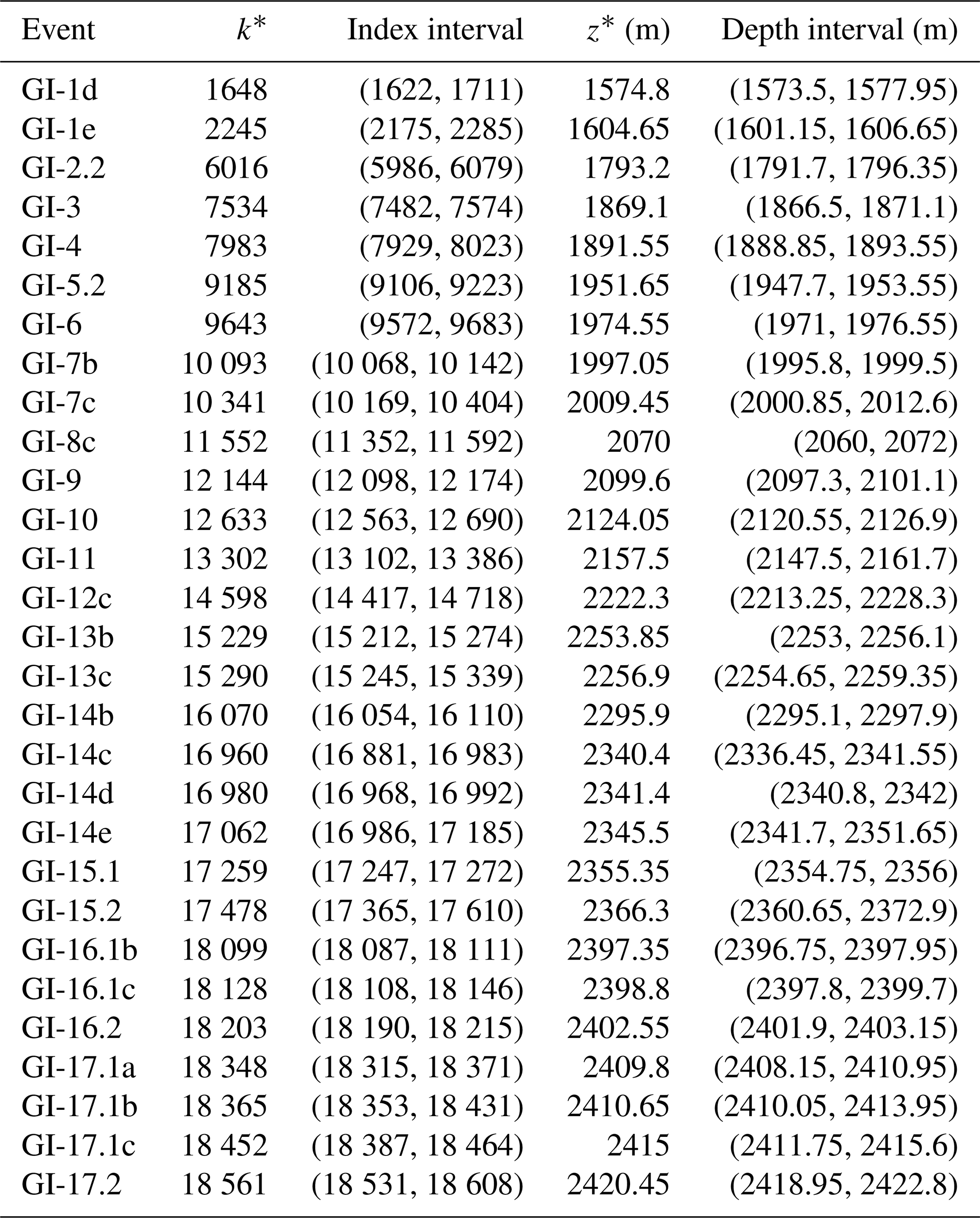
First, we adopt the Bayesian transition onset detection designed by Erhardt et al. (2019) to estimate the onset of the abrupt warming transitions in the proxy records with respect to the depth in the core. By Z^∗ we denote a continuous stochastic variable that represents the uncertain onset depth and by x^∗ we denote a selected data window of the proxy record enclosing the transition. For each transition this yields a posterior distribution $\mathit{\pi }\left(Z^{\ast }\right|{\mathit{x}}^{\ast })$ over potential transition onset depths, assuming a linear transition from low to high proxy values perturbed by AR(1) noise. For inference we adopt the methodology of INLA as it is particularly suited for such models, granting us a significant reduction in computational cost over traditional MCMC algorithms. The application of the transition onset detection to the onset of GI-11 is presented in Fig. 6a, with the resulting posterior marginal distribution for Z^∗ illustrated in Fig. 6b. Note that the dating method for the transitions is sensitive to the choice of the data window. In Appendix D we detail how the fitting windows for the linear ramps are optimally chosen. The selected data windows are listed in Table D1. Furthermore, the Bayesian transition detection fails in some cases where the transition amplitudes are small. We successfully derive posterior marginal distribution for a total of 29 events, whose summary statistics are listed in Table 1.

Table 1 Linear ramp model fits for the NGRIP depth of 29 abrupt warming events, as well as the full dating uncertainty. Data include the depth z^* and dating y^* from Rasmussen et al. (2014), as well as the posterior marginal mean and 95 % credible intervals for the estimated onset depth Z^* and age Y^*.

Each potential transition onset depth z^* yields a distribution over potential transition onset ages Y^*. This uncertainty, denoted by $\mathit{\pi }\left(Y^{*}\right|\mathrm{\Delta }\mathit{y},z^{*})$, is determined by linearly interpolating the age ensemble members generated according to Sect. 3.1 based on the observed layer increments Δy. The posterior distribution for the transition onset date for a given DO event thus reads

$$\begin{array}{}\text{(22)}& \mathit{\pi }\left(Y^{*}|\mathrm{\Delta }\mathit{y},{\mathit{x}}^{*}\right)=\int \mathit{\pi }\left(Y^{*}|\mathrm{\Delta }\mathit{y},Z^{*}\right)\mathit{\pi }\left(Z^{*}|{\mathit{x}}^{*}\right)\mathrm{d}{Z}^{*}.\end{array}$$

Technically, we create an ensemble of potential onset ages in the following way: First, we generate an ensemble of 10 000 samples from the posterior distribution of the transition onset depth,

$$z_r^{*}\sim \mathit{\pi }(Z^{*}\mid {\mathit{x}}^{*}),r\in [\mathrm{1},\mathrm{10}\mathrm{000}],$$

to represent the onset depth uncertainty. Second, for each onset depth sample $z_r^{*}$ we produce a simulation of a chronology from the corresponding age uncertainty:

$$y_r^{*}|z_r^{*}\sim \mathit{\pi }(Y^{*}|\mathrm{\Delta }\mathit{y},z_r^{*}).$$

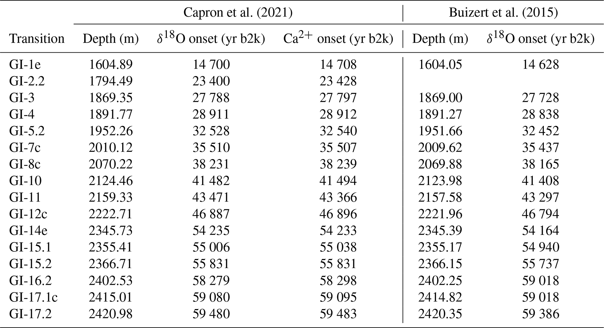
Thus, for both proxies (δ¹⁸O and Ca²⁺) and for each event we obtain 10 000 possible values for the transition onset age whose distribution corresponds to the posterior distribution expressed in Eq. (22). The posterior marginal mean and 95 % credible intervals for each event are reported in Table 1. This table hence gives the timing of the transitions together with the full uncertainties, stemming from the transition onset detection and the dating of the record. The estimated dating uncertainties are presented visually in Fig. 7, where they are also compared to the onset age obtained by Rasmussen et al. (2014), as well as the best estimates from Buizert et al. (2015) and Capron et al. (2021) which are presented in Table 2.

Capron et al. (2021)Buizert et al. (2015)

Table 2 Greenland interstadial transitions observed in the NGRIP record. Data include the median onset NGRIP depth and age for the δ¹⁸O and Ca²⁺ proxy records as reported in Capron et al. (2021) and the δ¹⁸O record presented in Buizert et al. (2015).

Although the GICC05 ages y^* of abrupt warming events and subevents as reported by Rasmussen et al. (2014) fall within our estimated 95 % credible intervals for all transitions, there are some transitions where there is a notable difference between the estimated posterior marginal mean E(Y^*) and the reported y^*. This can be partially explained by the fact that Rasmussen et al. (2014) uses a lower 20-year temporal resolution, and that they determine the onset from three different ice cores and two different proxies (δ¹⁸O and Ca²⁺), whereas our assessment is based on the univariate NGRIP proxy records only. With $E\left(Y^{*}\right)-y^{*}\sim \mathrm{120}$ the difference is most prominent in the GI-11 transition, whose simulated ages are represented in the histogram in Fig. 6c. This discrepancy is caused by the difference between our estimated onset depth Z^* and z^* from our linear ramp model fit shown in Fig. 6a. Our estimated onset depth E(Z^*) differs from the value z^* reported by Rasmussen et al. (2014) by approximately 1.6 m. This discrepancy propagates into an accordingly large difference in the age estimation of the transition onset. This demonstrates the importance of incorporating proper estimation and uncertainty quantification of the onset depth. Although the absolute uncertainty added from determining the onset depth can be considered negligible compared with the much larger age–depth uncertainty, there can still be a noticeable shift in the estimated onset age propagated from the estimation of the onset depth.

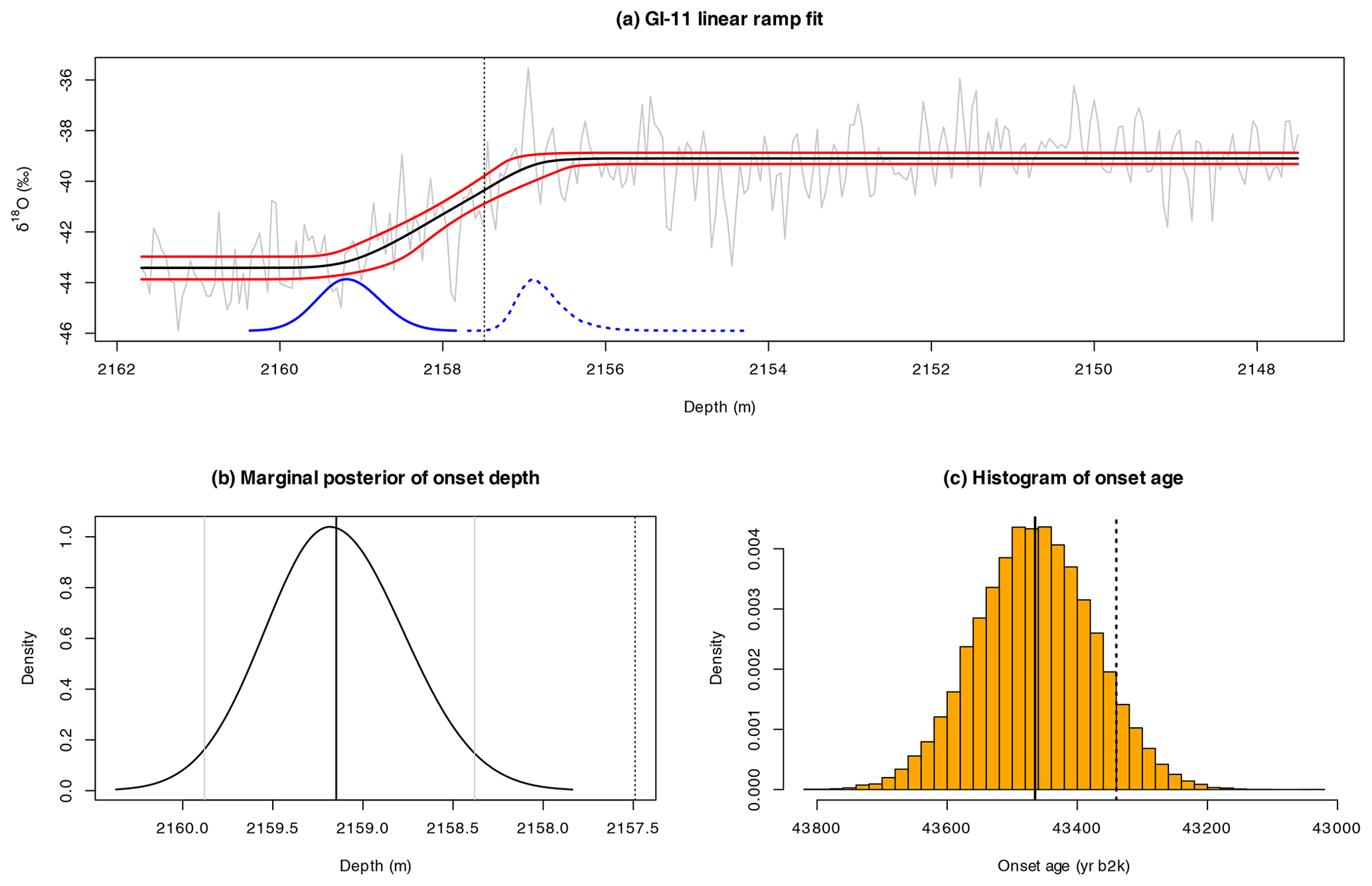
Figure 6 (a) The recorded δ¹⁸O of the NGRIP data x^* (gray) as a function of depth for the GI-11 transition. The black line represents the posterior marginal mean of the linear ramp model fitted using INLA. The enclosing red lines represent the corresponding 95 % credible intervals. The blue curves at the bottom illustrate the (unscaled) posterior distributions of the onset (solid) and end point (dotted) of the transition. The vertical dotted line represents the onset depth z^* as reported in Rasmussen et al. (2014). (b) The posterior marginal distribution of the onset depth Z^* following a linear ramp model fit. The solid vertical lines represent the posterior marginal mean (black) and 95 % credible intervals (gray). The dotted vertical line represents z^*. (c) Histogram describing the complete dating uncertainty of the transition to GI-11, taking into account the uncertainty of the NGRIP depth of the onset as well as the dating uncertainty at this depth. The solid vertical black line represents the mean of these samples, E(Y^*), and the dotted vertical line represents the GICC05 onset age y^* as reported in Rasmussen et al. (2014).

Figure 7 Posterior distributions of the onset ages of abrupt climate transitions for the NGRIP δ¹⁸O (black) and Ca²⁺ (gray) proxy records. The results are compared with ages reported by Rasmussen et al. (2014) (blue), Buizert et al. (2015) (green), and Capron et al. (2021) (red and pink for the δ¹⁸O and Ca²⁺ record, respectively). The Ca²⁺-based posterior distributions rely on modeled chronologies which are presented in Appendix B and which are not shown in the main text.

5 Discussion

Motivated by the relationship between air temperature on the one hand and the water-holding capacity and thus precipitation on the other hand, we assumed a linear dependency of the number of incremental layers per 5 cm on respective values of δ¹⁸O, which serves as an air temperature proxy. The only other climate proxy variable which is available from the NGRIP ice core at the same resolution over the same time period is the Ca²⁺ particle concentration (Ruth et al., 2003). From visual inspection one can already see that the negative logarithm of the Ca²⁺ mass concentration record shows high covariability with the δ¹⁸O record (see, for example, Fig. 1 of Rasmussen et al. (2014)). Changes in the Ca²⁺ concentrations are interpreted as changes in the local and hemispheric atmospheric circulation (e.g., Ruth et al., 2007; Schüpbach et al., 2018; Erhardt et al., 2019), which would also affect the amount of precipitation over Greenland. Above, we have focused on the δ¹⁸O; and analogous analysis for $-\log {\mathrm{Ca}}^{\mathrm{2}+}$ is presented in Appendix B. The results of the $-\log {\mathrm{Ca}}^{\mathrm{2}+}$-based chronology modeling are in very good agreement with the ones based on δ¹⁸, which corroborates our methodology.

Adopting Gaussian noise models in principle allows for a negative modeled number of incremental layers in a 5 cm incremental core segment, which does not seem plausible from a physical perspective. To avoid this, for comparison one could log-transform the age increments and then apply the modeling procedure. The model output would then have to be transferred back by taking the exponential. However, it turns out that the log transformation induces systematic deviations of the mean model output age from the reported GICC05 age. With the chances of negative layer increments being fairly small (less than 5 %), overall the original model outperforms the log-transformed model. A more detailed discussion on the log-transformed modeling approach is given in Appendix C.

From Fig. 2b we observe that the variance of the residuals increases slightly with increasing depth down in the core. This heteroskedasticity can be incorporated into our latent Gaussian model by assuming that the variance depends on the core depth in some predefined way. As this implementation is rather technical we consider it beyond the scope of the current paper. Regardless, assuming constant variance appears to be a good first order approach.

6 Conclusions

We have developed a general statistical framework for quantifying the age–depth uncertainty of layer counted proxy archives. In these records the age can be determined by counting annual layers that result from seasonal variations, which in turn impact the deposition process. By counting these layers one can assign time stamps to the individual proxy measurements. However, there is a non-negligible uncertainty associated with this counting process. Proper quantification of this uncertainty is important since it carries valuable information and the error propagates to further analyses, e.g., dating of climatic events, determining cause and effect between such events, and model-data comparisons. Originally, the uncertainty of the GICC05 is quantified in terms of the maximum counting error (MCE), defined as half the number of uncertain layers. However, since this method assumes that uncertain layers are either true or false, we believe this to be an overly conservative estimate, giving too high uncertainty for deeper layers.

In our approach we express the number of layers per depth increment as the sum of a structured component and a stochastic component. The structured component represents physical layer thinning, a positive temperature–precipitation feedback, and persisting trends over individual stadials and interstadials. The stochastic component takes into account the natural variability of the layer thickness and the errors made in the counting process. After fitting the structured component in a least squares manner, we find the residuals to be approximately stationary, Gaussian distributed, and to exhibit short-range autocorrelation. These summary statistics motivate us to employ Gaussian white noise, or an autoregressive process of first or second order, as the stochastic part of the age–depth model.

After defining the structure of the model, we estimate all model parameters simultaneously in a hierarchical Bayesian framework. The resulting joint posterior distribution on the one hand serves as a quantification of the parameter uncertainty in the model and on the other hand allows to generate chronology ensembles that reflect the uncertainty in the age–depth relationship of the NGRIP ice core. The dating uncertainties obtained from this approach are significantly smaller than those from the MCE. We also find that our estimates do not deviate much from the GICC05 in terms of best estimates for the dating.

Additional information that may help to further constrain the uncertainties, such as tie points obtained via cosmogenic radionuclides (Adolphi et al., 2018), will be fed into the model in future research.

One of the biggest concerns regarding the layer counting is that of a potential counting bias. Such a systematic error cannot be corrected after the counting and, therefore, we investigate how a potential unknown counting bias increases the uncertainty of the presented age–depth model. If such a counting bias is restricted to ±4 % we obtain total age uncertainties comparable to the estimates based on the MCE. Finally, we apply our method to the dating of DO events. Using a Bayesian transition onset detection we are able to combine the uncertainty of the onset depth with the corresponding age uncertainty, and to give a posterior distribution that entails the complete dating uncertainty of each transition onset. We find that previous estimates of the DO onsets reported in Rasmussen et al. (2014) are well within our estimated uncertainty ranges both in terms of depth and age. However, the dating uncertainties of the abrupt warming event onsets are all considerably smaller than the MCE, even when accounting for the additional uncertainty associated with the onset depth.

In theory, it should be possible to apply this approach to other layered proxy records as well. However, there are some requirements that need to be fulfilled for this approach to be applicable. The first condition is that a potential layer thinning can be adequately expressed by a regression model. In our results we find the residuals to follow a Gaussian process, but it should be possible for the model to be adapted such that it supports other distributions for the residuals as well. However, depending on the model, if the residuals exhibit too long memory then this could lead to the simulation procedure having an infeasibly high computational cost. Moreover, if there are many effects in the regression model there needs to be sufficient data to achieve proper inference.

Appendix A: Latent Gaussian model formulation

In this study we consider different Gaussian models for the noise component, including independent identically distributed (iid) and first and second order autoregressive (AR) models. These models all exhibit the Markov property, meaning there is a substantial amount of conditional independence. So-called Gaussian Markov random fields are known to work really well with the methodology of integrated nested Laplace approximations (INLAs), which will grant a substantial reduction in computational cost in obtaining full Bayesian inference. However, this requires formulating our model into a latent Gaussian model where the data, here $\mathcal{D}=(\mathrm{\Delta }{y}_{\mathrm{1}},\mathrm{\dots },\mathrm{\Delta }{y}_n{)}^{\top }$, depend on a set of latent Gaussian variables $\mathit{X}=(X_{\mathrm{1}},\mathrm{\dots },X_N{)}^{\top }$ which in turn depend on hyperparameters $\mathit{\theta }=({\mathit{\theta }}_{\mathrm{1}},\mathrm{\dots },{\mathit{\theta }}_m{)}^{\top }$. This class of models constitutes a subset of hierarchical Bayesian models and is defined in three stages.

The first stage defines the likelihood of the data and how they depend on the latent variables. For the data and models used in this study we assume a direct correspondence between an observation y_i and the corresponding latent variable X_i, which is achieved using a Gaussian likelihood with some negligible fixed variance and mean given by the linear predictor,

$${\mathit{\eta }}_k=E\left(\mathrm{\Delta }{y}_k\right)=b{z}_k^{\mathrm{2}}+b_x{x}_k+\sum _{i=\mathrm{1}}^p{\mathit{\psi }}_i(z_k;a_i,c_i)+{\mathit{\epsilon }}_k\left(\mathit{\theta }\right).$$

Here, $\mathit{\beta }=(b_{\mathrm{0}},b,b_x,\mathit{\{}{a}_i\mathit{\}},\mathit{\{}{c}_i\mathit{\left\}}\right)$ are known as fixed effects, even though they are indeed stochastic variables in the Bayesian framework. The noise variables ε_k(θ) are referred to as random effects since they depend on hyperparameters θ. The hyperparameters are θ=σ_ε if we assume the residuals follow an iid Gaussian process, $\mathit{\theta }=({\mathit{\sigma }}_{\mathit{\epsilon }},\mathit{\varphi })$ if they follow an AR(1) process, and $\mathit{\theta }=({\mathit{\sigma }}_{\mathit{\epsilon }},{\mathit{\varphi }}_{\mathrm{1}},{\mathit{\varphi }}_{\mathrm{2}})$ if they follow an AR(2) process. All random terms in the predictor, and the predictor itself, are included in the latent field $\mathit{X}=(\mathit{\eta },\mathit{\beta },\mathit{\epsilon })$. The latent field is assigned a prior distribution in what is the second stage of defining a latent Gaussian model. For latent Gaussian fields this prior is multivariate Gaussian:

$$\mathit{X}\mid \mathit{\theta }\sim \mathcal{N}\left(\mathit{\mu }\left(\mathit{\theta }\right),\mathbf{\Sigma }\left(\mathit{\theta }\right)\right).$$

Specifically, we assume vague Gaussian priors for β, while the prior for ε(θ) is either an iid, AR(1), or AR(2) process. The predictor η is then a Gaussian with a mean vector corresponding to the linear regression a(β) and a covariance matrix given by the covariance structure of the assumed noise model.

The third and final stage of the latent Gaussian model definition is to specify a prior distribution on the hyperparameters. We use the default prior choices included in the R-INLA package, which means that for all models of ε considered in this paper the scaling parameter ${\mathit{\sigma }}_{\mathit{\epsilon }}^{\mathrm{2}}$ is assigned a log-gamma distribution through the transformation $\mathit{\kappa }=\mathrm{1}/{\mathit{\sigma }}_{\mathit{\epsilon }}^{\mathrm{2}}$. When the residuals follow an AR(1) distribution we assume a Gaussian prior on the additional lag-one correlation parameter using a logit transformation $\mathit{\rho }=\log \left(\right(\mathrm{1}+\mathit{\varphi })/(\mathrm{1}-\mathit{\varphi }\left)\right)$. For the AR(2) residuals we instead assign penalized complexity priors (Simpson et al., 2017) on the partial autocorrelations ${\mathit{\psi }}_{\mathrm{1}}={\mathit{\varphi }}_{\mathrm{1}}/(\mathrm{1}-{\mathit{\varphi }}_{\mathrm{2}})$ and ψ₂=ϕ₂, also using a logit transformation.

Inference is obtained by computing the posterior marginal distributions:

$$\mathit{\pi }\left(X_k\right|\mathcal{D})=\int \mathit{\pi }\left(X_k|\mathit{\theta },\mathcal{D}\right)\mathit{\pi }(\mathit{\theta }\left|\mathcal{D}\right)\mathrm{d}\mathit{\theta }$$

and

$$\mathit{\pi }\left({\mathit{\theta }}_k|\mathcal{D}\right)=\int \mathit{\pi }\left(\mathit{\theta }\right|\mathcal{D})\mathrm{d}{\mathit{\theta }}_{-k}.$$

The notation θ_k refers to the kth hyperparameter, and θ_−k refers to all except the kth hyperparameter. These integrals can be approximated efficiently using R-INLA, and the resulting posterior marginal distributions are included in Fig. A1. The estimated hyperparameter posterior marginal means and credible intervals (given in parentheses) are ${\mathit{\sigma }}_{\mathit{\epsilon }}^{\mathrm{iid}}\approx \mathrm{0.427}$ (0.423, 0.431) for iid residuals, ${\mathit{\sigma }}_{\mathit{\epsilon }}^{\mathrm{AR}}\left(\mathrm{1}\right)\approx \mathrm{0.428}$ (0.423, 0.434) and ϕ^AR(1)≈0.194 (0.178,0.217) for AR(1) residuals, and ${\mathit{\sigma }}_{\mathit{\epsilon }}^{\mathrm{AR}}\left(\mathrm{2}\right)\approx \mathrm{0.429}$ (0.423, 0.438), ${\mathit{\varphi }}_{\mathrm{1}}^{\mathrm{AR}}\left(\mathrm{2}\right)\approx \mathrm{0.180}$ (0.158, 0.210), and ${\mathit{\varphi }}_{\mathrm{2}}^{\mathrm{AR}}\left(\mathrm{2}\right)\approx \mathrm{0.108}$ (0.089, 0.134) for AR(2) residuals.

Figure A1 The posterior marginal distributions obtained by fitting the model with INLA. Panel (a) shows the density of σ_ε using iid distributed residuals. Panels (b) and (c) show the densities of σ_ε and ϕ using AR(1) distributed residuals. Panels (d)–(f) show the densities of σ_ε,ϕ₁, and ϕ₂ using AR(2) distributed residuals. The vertical lines represent the mean (black) and 95 % credible intervals (gray).

Appendix B: Ca²⁺ analysis

As an alternative, we perform an analogous study using the log(Ca²⁺) as the proxy variable x_k, which is available at the same period and resolution (Ruth et al., 2003). Missing values in the Ca²⁺ data set are filled using linear interpolation. Performing the same analysis as described in Sect. 3 we produce joint samples of the chronologies. The resulting posterior marginal means and 95 % credible intervals of the dating uncertainties are illustrated in Fig. B1, where the credible intervals obtained using an iid, AR(1), and AR(2) noise model are compared. These results are consistent with those obtained using δ¹⁸O as the proxy variable, shown in Fig. 4.

Figure B1 The 95 % credible intervals of the dating uncertainty distribution when log(Ca²⁺) is used as the proxy covariate. The GICC05 time scale has been subtracted and the noise is modeled using iid (black), AR(1) (blue), and AR(2) (red) noise models. Only the posterior marginal mean computed using AR(1) distributed noise is included (gray) since it is very similar to the mean obtained using other noise assumptions.

Appendix C: Log-normal distribution

A possible concern with the approach presented above is that assuming a normal distribution on the layer increments assigns a non-zero probability of negative depositions, violating monotonicity. Furthermore, one might be concerned by our choice of an additive thinning function rather than a multiplicative. Both of these issues are resolved by instead assuming a log-normal regression model on the layer increments, i.e.,

$$\begin{array}{}\text{(C1)}& \log \mathrm{\Delta }{y}_k=a\left(z_k,x_k\right)+{\mathit{\epsilon }}_k,\end{array}$$

where ε_k follows either an iid, AR(1), or AR(2) model as before. This results in the joint age variables being a multivariate process with marginals described by sums of log-normal distributions.

Simulations of the chronology can be produced as follows: First, the latent Gaussian model is fitted to the data and second, a(z_k,x_k) and ε_k are sampled from the resulting posterior distributions. Then compute the sampled chronologies:

$$\begin{array}{}\text{(C2)}& y_k=y_{\mathrm{0}}+\sum _{i=\mathrm{1}}^k\exp \left(a\left(z_i,x_i\right)+{\mathit{\epsilon }}_i\right).\end{array}$$

The resulting dating uncertainty is illustrated in Fig. C1 and is more curved than for the original model. This suggests that the normal distribution is a better fit to the observed layer increments. We will hence focus on the original Gaussian model in the analysis of this paper.

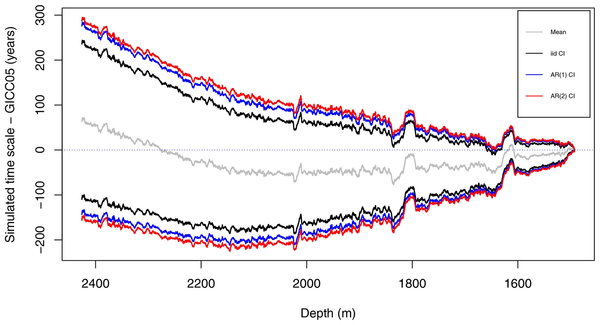
Figure C1 The 95 % credible intervals of the dating uncertainty distribution when the GICC05 time scale has been subtracted and a log-normal distribution is assumed, using iid (black), AR(1) (blue), and AR(2) (red) noise models. Only the posterior marginal mean computed using AR(1) distributed noise is included (gray) since it is very similar to the mean obtained using the other noise models.

Appendix D: Determination of the fitting windows

The estimation for the onset depth is sensitive to the choice of the data window which represents the transition. It is important to select these carefully such that the data best represent a single linear ramp function while being of a sufficient size. As some DO events are located more closely to other transitions than others, it is necessary to determine these data windows individually for each transition. As such there are indeed some transitions where it is difficult to determine a clear transition point, and a linear ramp model is not appropriate. These transitions will be omitted from our analysis. The reduction in computational cost granted by adopting the model for INLA allows us to perform repeated fits to determine the optimal data interval based on a given criteria. Specifically, we adjust both sides of the interval until we find the data window for which the fitted model yields the lowest amplitude of the AR(1) noise, measured by the posterior marginal mean of the standard deviation parameter.

We impose some restrictions on the domain of the optimal start and end points of our data interval. To achieve the best possible fit we want our interval to include both the onset and end point of the transition, which we suspect are located close to the NGRIP onset depth z^* given by Table 2 of Rasmussen et al. (2014). Unless the DO events are located too close to adjacent transitions, we assume the optimal interval always contains the points representing 1 m above to 2.5 m deeper than z^*. These are the minimum distances from the proposed onset. Similarly, we also introduce a maximum distance from z^* to be considered for the start and end points of the data interval. This is set to be 10 m above and 15 m deeper than z^*, or at the adjacent transitions if they are located closer than this. From these intervals we create a two-dimensional grid for which we perform the INLA fit for each grid point. The start and end points of the interval representing the grid point for which INLA found the lowest noise amplitude are selected. Those events that failed to provide a decent fit after the conclusion of this procedure were discarded. This left us with 29 DO events for which the results are displayed in Table D1. Although the GICC05 onset depths z^* fall outside the 95 % credible intervals for several transitions, they are still remarkably close to our best estimates, considering Rasmussen et al. (2014) used a lower 20 year resolution data set.

Table D1 The optimal interval for the data window for fitting a linear ramp model to 29 DO events, expressed in terms of depth and the corresponding index in our data. The Rasmussen et al. (2014) onset depths z^* were used as a starting midpoint in the optimization procedure.