the Creative Commons Attribution 4.0 License.
the Creative Commons Attribution 4.0 License.
 | 05 May 2021
Comparison of the oxygen isotope signatures in speleothem records and iHadCM3 model simulations for the last millennium
Janica C. Bühler
Carla Roesch
Moritz Kirschner
Louise Sime
Max D. Holloway
Kira Rehfeld
Improving the understanding of changes in the mean and variability of climate variables as well as their interrelation is crucial for reliable climate change projections. Comparisons between general circulation models and paleoclimate archives using indirect proxies for temperature or precipitation have been used to test and validate the capability of climate models to represent climate changes. The oxygen isotopic ratio δ18O, a proxy for many different climate variables, is routinely measured in speleothem samples at decadal or higher resolution, and single specimens can cover full glacial–interglacial cycles. The calcium carbonate cave deposits are precisely dateable and provide well preserved (semi-)continuous albeit multivariate climate signals in the lower and mid-latitudes, where the measured δ18O in the mineral does not directly represent temperature or precipitation. Therefore, speleothems represent suitable archives to assess climate model abilities to simulate climate variability beyond the timescales covered by meteorological observations (101–102 years).
Here, we present three transient isotope-enabled simulations from the Hadley Center Climate Model version 3 (iHadCM3) covering the last millennium (850–1850 CE) and compare them to a large global dataset of speleothem δ18O records from the Speleothem Isotopes Synthesis and AnaLysis (SISAL) database version 2 (Comas-Bru et al., 2020b). We systematically evaluate offsets in mean and variance of simulated δ18O and test for the main climate drivers recorded in δ18O for individual records or regions.
The time-mean spatial offsets between the simulated δ18O and the speleothem data are fairly small. However, using robust filters and spectral analysis, we show that the observed archive-based variability of δ18O is lower than simulated by iHadCM3 on decadal and higher on centennial timescales. Most of this difference can likely be attributed to the records' lower temporal resolution and averaging or smoothing processes affecting the δ18O signal, e.g., through soil water residence times. Using cross-correlation analyses at site level and modeled grid-box level, we find evidence for highly variable but generally low signal-to-noise ratios in the proxy data. This points to a high influence of cave-internal processes and regional climate particularities and could suggest low regional representativity of individual sites. Long-range strong positive correlations dominate the speleothem correlation network but are much weaker in the simulation. One reason for this could lie in a lack of long-term internal climate variability in these model simulations, which could be tested by repeating similar comparisons with other isotope-enabled climate models and paleoclimate databases.
- Article
(7924 KB) - Full-text XML
-
Supplement
(27324 KB) - BibTeX
- EndNote


The impacts of a changing climate have been observed over the last century (IPCC, 2013) and indicate a strong sensitivity of human societies and natural systems to changes in climate. While the mean state of the climate is well observed, direction and magnitude of potential changes to its variability are still largely unclear (Franzke et al., 2020). However, changes in variability influence the occurrence of extreme temperature and precipitation events (Katz and Brown, 1992) and have major impacts on society, economies (Hänsel et al., 2020), and ecosystems (Vasseur et al., 2014).
Past climate changes provide a testbed to evaluate climate models and to better understand projected changes in the future (Schmidt et al., 2012; Braconnot et al., 2012). Instrumental records only cover a short period of time, since systematic observations of climate variables only began in 1750 CE (black line in Fig. 1a, Morice et al., 2012). For model evaluation on longer than centennial timescales, we have to rely on evidence from paleoclimate archives, such as trees, ice cores, foraminifera from marine sediment cores, or speleothems. The abundance of the heavy oxygen isotope 18O, further denoted as δ18O, is a proxy for many climate variables and can be measured on these and quite a few other paleoclimate archives with high precision (Schmidt et al., 2014). The climatic interpretation of δ18O changes, however, are not always straightforward (Fairchild and Baker, 2012). Speleothem archives, which we rely on here, allow sampling of a wide range of climates in the low latitudes to mid-latitudes and provide (semi-)continuous precisely dated time series of oxygen isotope ratios.
Few other transient model–data comparison studies focused on δ18O (e.g., Wackerbarth et al., 2012; Dee et al., 2015; Colose et al., 2016; Stevenson et al., 2019; Parker et al., 2020). For example, Sjolte et al. (2018) compared the variability of the simulated ECHAM5/MPI-OM δ18O to Greenland ice cores over the last millennium, assimilating the ice core data to produce gridded reconstructions. They were able to differentiate between solar and volcanic forcing effects from their reconstructions. On orbital timescales (150 000 years), Caley et al. (2014) compared a transient isotope-enabled simulation with a model of intermediate complexity (iLOVECLIM) to speleothem records from Southeast Asia. They found model–data similarity for the broad temporal trends, but differences at shorter timescales, highlighting the role of seasonality.
For our model–data comparison, we focus on the time period of the last millennium (850–1850 CE; Taylor et al., 2012), for which a fairly high number of well-preserved datasets are available. This time period is characterized by stable, close-to-present-day boundary conditions (fairly constant greenhouse gas concentrations and sea level) and climate variability due to natural, solar, and volcanic forcings (Schurer et al., 2014; PAGES2k-Consortium, 2019; Taylor et al., 2012; Neukom et al., 2019). It is also one of the key paleoclimate periods included in the joint experiments of the Paleoclimate Model Intercomparison Project Phase 3 and 4 (PMIP3/PMIP4; Jungclaus et al., 2010; Kageyama et al., 2018) and the overarching Coupled Model Intercomparison Project Phase 5 and 6 (CMIP5/CMIP6; Taylor et al., 2012; Eyring et al., 2016).
Modeled climate variability can be a consequence of either internal interactions and processes (internal variability) or of radiative forcings such as depicted in Fig. 1c–e (forced external variability), e.g., greenhouse gases, volcanic eruptions, or total solar irradiance.
Previous studies have suggested that simulated temperature variability is systematically too low on decadal and longer timescales, especially on the regional scale (Laepple and Huybers, 2014a). This has been attributed to models being too diffusive, denoting energy being dissipated too quickly across temporal scales (Laepple and Huybers, 2014b), or to missing processes and feedbacks (Rehfeld et al., 2016). Variability induced by external radiative forcing only accounts for a small fraction of the regional climate variance (Goosse et al., 2005; Laepple and Huybers, 2014b). Discrepancies increase towards longer timescales (Laepple and Huybers, 2014a) and are already substantial at the multidecadal to centennial timescales that we target here.
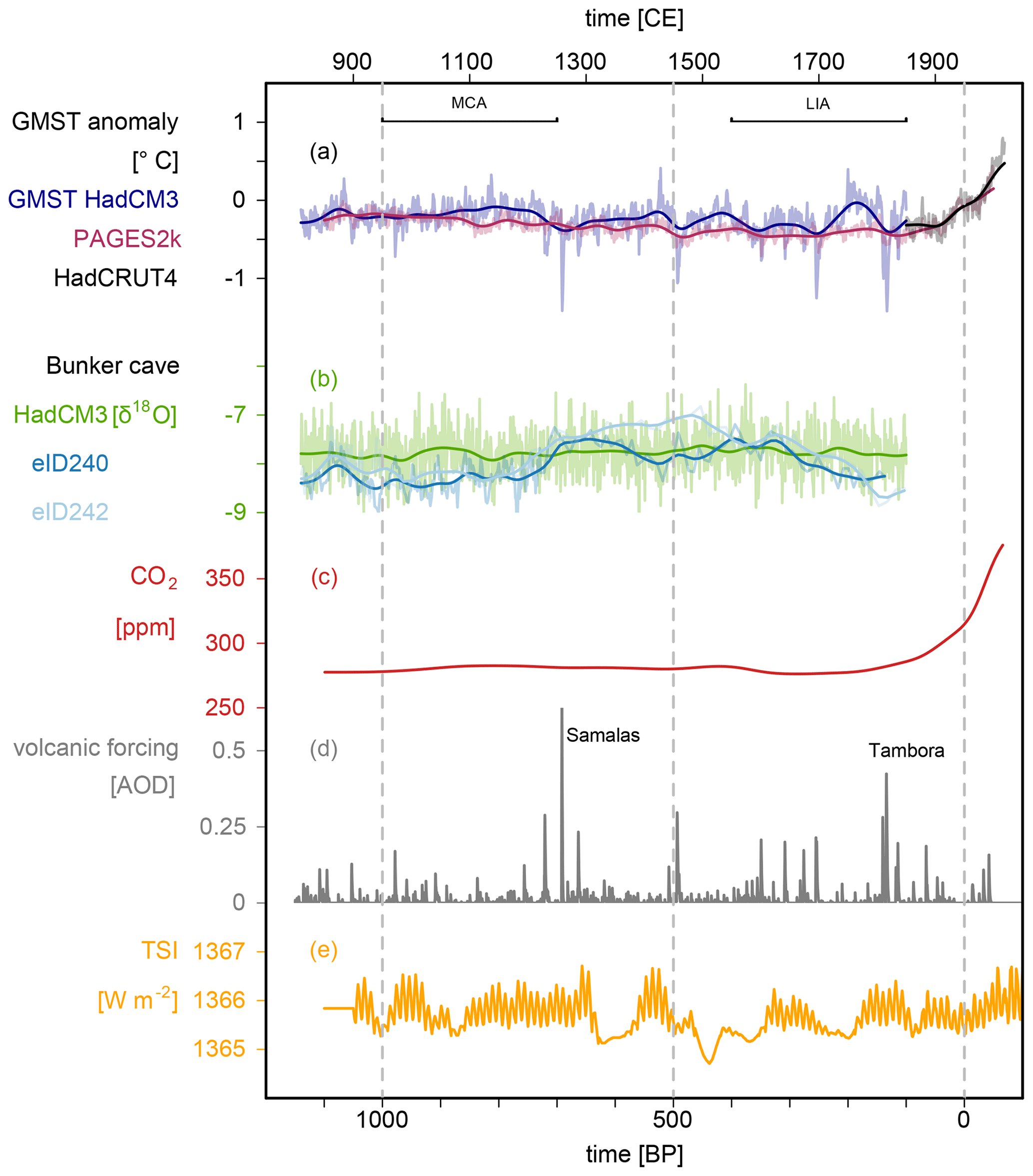
Figure 1Climate and main climatic drivers over the last millennium. (a) Global annual mean surface temperature (GMST) as modeled (iHadCM3, blue), reconstructed (PAGES2k, red) (PAGES2k-Consortium, 2019), and observed (HadCRUT4, black) (Morice et al., 2012). (b) Annual mean δ18O in precipitation at Bunker Cave, Germany, as modeled (iHadCM3, green) and measured calcite δ18O (drip water equivalent) from SISAL entity 240 (dark blue) and 242 (light blue) at the Bunker cave site (Comas-Bru et al., 2019; Fohlmeister et al., 2012). Comparison plots for all entities are given in Figs. S1–S2 in the Supplement. (c) Atmospheric CO2 concentration, (d) volcanic forcing in units of aerosol optical depth (AOD) (Crowley and Unterman, 2013), and (e) total solar irradiance (TSI) as used in the model simulations (Steinhilber et al., 2009; Wang et al., 2005).
The incorporation of an isotopic water cycle into isotope-enabled general circulation models (iGCMs) provides additional means for understanding the hydrology of the climate system (Werner et al., 2016; Sturm et al., 2010; Tindall et al., 2009). The ratio of H218O to H216O in precipitation is an indicator of evaporation temperature, precipitation amount, and altitude, as well as distance to source water (Dansgaard, 1964). It is given in the δ notation as
where standard indicates the Vienna Standard Mean Ocean Water standard V-SMOW (Kendall and Caldwell, 1998).
On monthly to decadal timescales, the Global Network of Isotopes in Precipitation (GNIP) database (IAEA/WMO, 2020) provides measurements of δ18O in collected precipitation water, which have been used in model–data comparisons for the present climate (Tindall et al., 2009; Werner et al., 2011; Comas-Bru et al., 2020b). On decadal and longer timescales, paleoclimate archives such as speleothems are crucial. δ18O variations in stalagmites, to first order, represent changes in δ18O in the meteoric precipitation above the cave.
Speleothem cave deposits form in karst regions (Fairchild and Baker, 2012) under climatic conditions spanning from extremely cold (Lauritzen and Lundberg, 1999) and very arid (Neff et al., 2001) to extremely hot and humid conditions (Partin et al., 2007). As a terrestrial climate archive, they are able to store information on continental climate changes. They form as a calcite or aragonite matrix from calcium dissolved in acidic drip water and hence archive the oxygen isotope from precipitation water in accumulated growth layers (Fairchild and Treble, 2009). δ18O can be regarded as a proxy, e.g., for surface temperature variations in higher latitudes or precipitation amount in the tropics (Dansgaard, 1964). The proxy signal is, however, overlaid with distinct observable signatures of source water evaporation, transportation over longer distances (Bradley, 1999; Dansgaard, 1964), and large-scale climate patterns of circulation such as for example the North Atlantic Oscillation (NAO) (e.g. Vinther et al., 2010) or the El-Niño–Southern Oscillation (ENSO) (Tindall et al., 2009). All these δ18O signatures in precipitation may be visible in speleothem records, including additionally fractionation processes involved in the calcite formation, which is primarily temperature-dependent (Urey, 1948; McCrea, 1950). The climatic interpretation of speleothem δ18O variations in calcite or aragonite (hereafter δ18Ospeleo) can be hampered by non-linear growth processes (Dreybrodt and Scholz, 2011) and multiple cave-specific parameters such as vegetation cover (Haude, 1954; Wackerbarth et al., 2010), karst (Jean-Baptiste et al., 2019), and inner cave processes (Fairchild et al., 2006), which influence δ18Ospeleo. Especially in the comparison between δ18Ospeleo of different speleothems, dating uncertainties complicate the assessment of climatic drivers, as they increase the uncertainty in pairwise comparisons and similarity estimates (Breitenbach et al., 2012; Rehfeld and Kurths, 2014). For speleothems, in particular, positive correlations to ice core δ18O, which is considered a proxy for temperature, have been reported (McDermott et al., 2001) but so have negative correlations to local annual mean temperatures at the cave site (e.g., Lauritzen and Lundberg, 1999). This highlights the complexity of the system and the potential regionality of the signal. In studies on drip water, δ18O and annual mean temperature, regions with different dominant climate controls could be distinguished (Baker et al., 2019).
Here, we present three new last-millennium isotope-enabled simulations from the iGCM version 3 of the Hadley Model (iHadCM3) and test how similar the δ18O variations in iHadCM3 and speleothem records are (Sect. 4.1). A characterization of the datasets and relevant forcing can be found in Fig. 1. The robustness of the findings and methods are evaluated over the last millennium, for which a large number of high-resolution proxy datasets from the SISAL v.2 database (Comas-Bru et al., 2020b) are available. Our key questions are as follows: (i) how similar are the modeled δ18O signatures to the speleothem records especially regarding variability, (ii) can we distinguish the main drivers for these signatures, and (iii) how representative are the speleothem records for their region? To address these questions, we explore similarities on both spatial and temporal scales, to distinguish patterns of the mean state (Sect. 4.1), the variability (Sect. 4.2 and 4.3), and the spatial representativity of speleothem climate records (Sect. 4.4 and 4.5). We examine the simulation's capability to simulate and the records' capability to capture variability on different timescales to improve our understanding of processes and uncertainties of both.
2.1 Model description and simulation overview
In this study, we use the coupled atmosphere–ocean isotope-enabled GCM iHadCM3, which has been widely used to simulate present and future climate (Sime et al., 2008; Tindall et al., 2009; IPCC, 2013), as well as for past climates such as the late Holocene and Last Glacial Maximum (Holloway et al., 2016), the last interglacial (Sime et al., 2009, 2013; Holloway et al., 2016, 2018), and the Eocene (Tindall et al., 2010).
The model consists of several components: the atmosphere model HadAM3 (Pope et al., 2000), the ocean model HadOM3 (Gordon et al., 2000), a sea ice model (Valdes et al., 2017), and a dynamic land surface and vegetation model (Cox, 2001). The atmospheric component is run at a horizontal resolution of 2.5∘ × 3.75∘ and has 19 vertical levels and time steps of 30 min. The oceanic output has a horizontal resolution of 1.25∘ × 1.25∘, 20 vertical levels, and time steps of 1 h. For the isotope-enabled version, water isotopes HD16O and H218O were added as two separate water species in the atmospheric model, and as tracers in the ocean model. Fixed isotope fractions are added to a fixed volume grid box of the ocean and experience changes due to evaporation, precipitation, and runoff through a virtual isotope flux, altering the δ18O ratio in the top level of the ocean accordingly (Tindall et al., 2009). The land surface and vegetation evolve dynamically and are based on TRIFFID (Cox, 2001) with time steps of 5 years.
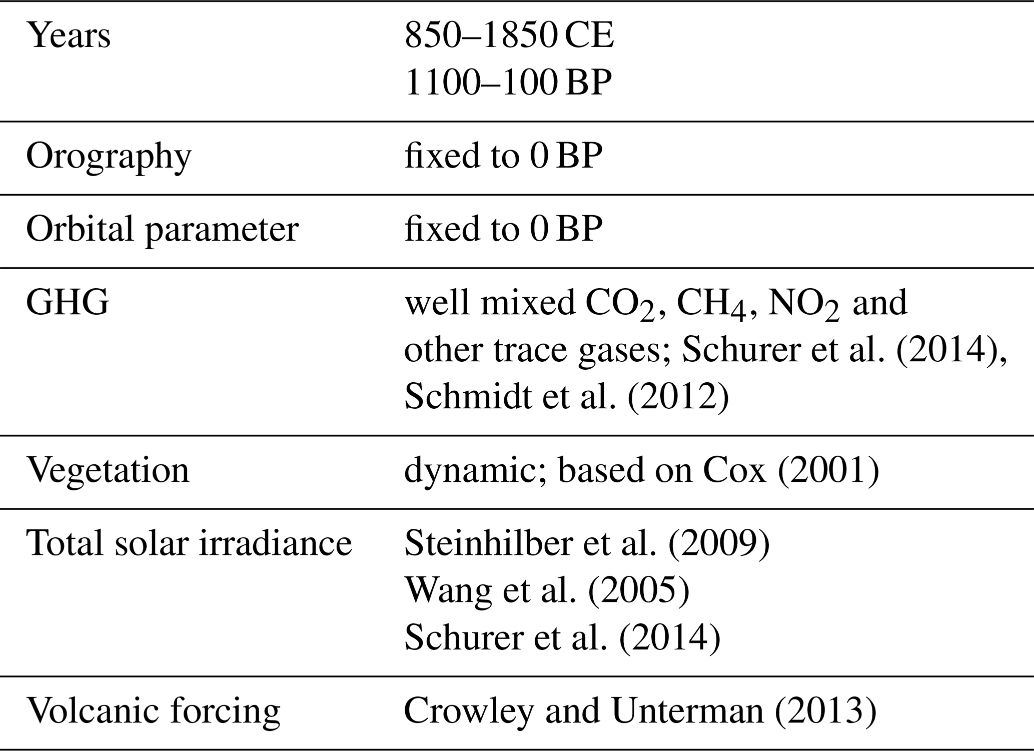
Compared to instrumental observations, the model represents sea surface temperature (SST), sea ice, and ocean heat content well (Gordon et al., 2000). The freshwater hydrological cycle in the model shows only a slight overestimation in the local evaporation (Pardaens et al., 2003). The model simulates the major isotopic fractionation effects as in Dansgaard (1964) (e.g., the latitude effect, the amount effect, and the continental effect) appropriately compared to GNIP data (Zhang et al., 2012). Additionally, a broad agreement in isotopic output with GNIP data in the general spatial distribution can be observed and the above-mentioned general oxygen isotopic ratio features are represented well (Tindall et al., 2009). As such, iHadCM3 captures large-scale features of climate and oxygen isotope ratios while remaining computationally efficient for the simulation of timescales such as the last millennium. The three ensemble members, which are identified with the LM prefix, were initialized from different years of the same spinup simulation. The basic characteristics and boundary conditions of the last-millennium simulations used in this analysis are listed in Table 1.
Schurer et al. (2014)Schmidt et al. (2012)Cox (2001)Steinhilber et al. (2009)Wang et al. (2005)Schurer et al. (2014)Crowley and Unterman (2013)Table 1Basic characterization of the LM1, LM2, and LM3 last-millennium simulations.
2.2 The speleothem isotope dataset
The oxygen isotope ratio measured in speleothems is subject to many processes, starting from the source water which is influenced by the atmospheric circulation and climate. Therefore, the amount of precipitation, its composition, the annual mean temperature, and the variability of these events are in part imprinted in the archive. A comprehensive summary of the processes involving speleothem growth can be found in Fairchild and Baker (2012).
Vegetation above the cave can alter the amount of infiltrating water and its isotopic signature, where the meteoric δ18O is subject to additional fractionation processes and seasonal effects (Haude, 1954; Thornthwaite and Mather, 1957; Wackerbarth et al., 2010). Filter processes and transportation through the soil and upper karst influence the signal and may lead to varying transit times between several minutes and multiple years (Jean-Baptiste et al., 2019) at different drip sites within the same cave. Infiltrating surface water is charged with soil gas CO2, where the partial CO2 pressure is larger than in the atmosphere, facilitating the carbonic acid-driven CaCO3 dissolution of the host rock. The generally lower partial pCO2 pressure conditions in the cave environment compared to that of the soil and epikarst makes the drip water degas and precipitate calcite in a fractionation process, which consequently forms a speleothem (Tremaine et al., 2011).
Varying environmental conditions within the cave can also be imprinted in the isotopic signal and may pronounce or attenuate the climate signal (Fairchild and Baker, 2012). During the calcification process, interactions with the cave environment or water inclusions within the mineral are still possible and, therefore, may further change the δ18Ospeleo archived in the speleothem.
The oxygen isotope composition of drip water is influenced by all above-mentioned factors. Due to the multivariate processes impacting speleothem growth, the interpretation of the δ18Ospeleo signal is not straightforward, although systematic evaluation has identified patterns of similar climate influence based on modern observations (Baker et al., 2019). Proxy system models (PSMs), where the input signal modification is modeled based on known processes in the karst, may also help with the interpretation (Evans et al., 2013; Dee et al., 2015). PSMs of varying complexity have been proposed from the simple exponential decay filter, mimicking karst mixing (Dee et al., 2015) with the delay time as the single tunable parameter, to full-blown karst system models with numerous parameters describing soil water and gas equilibration or carbonate bedrock dissolution (Owen et al., 2018).
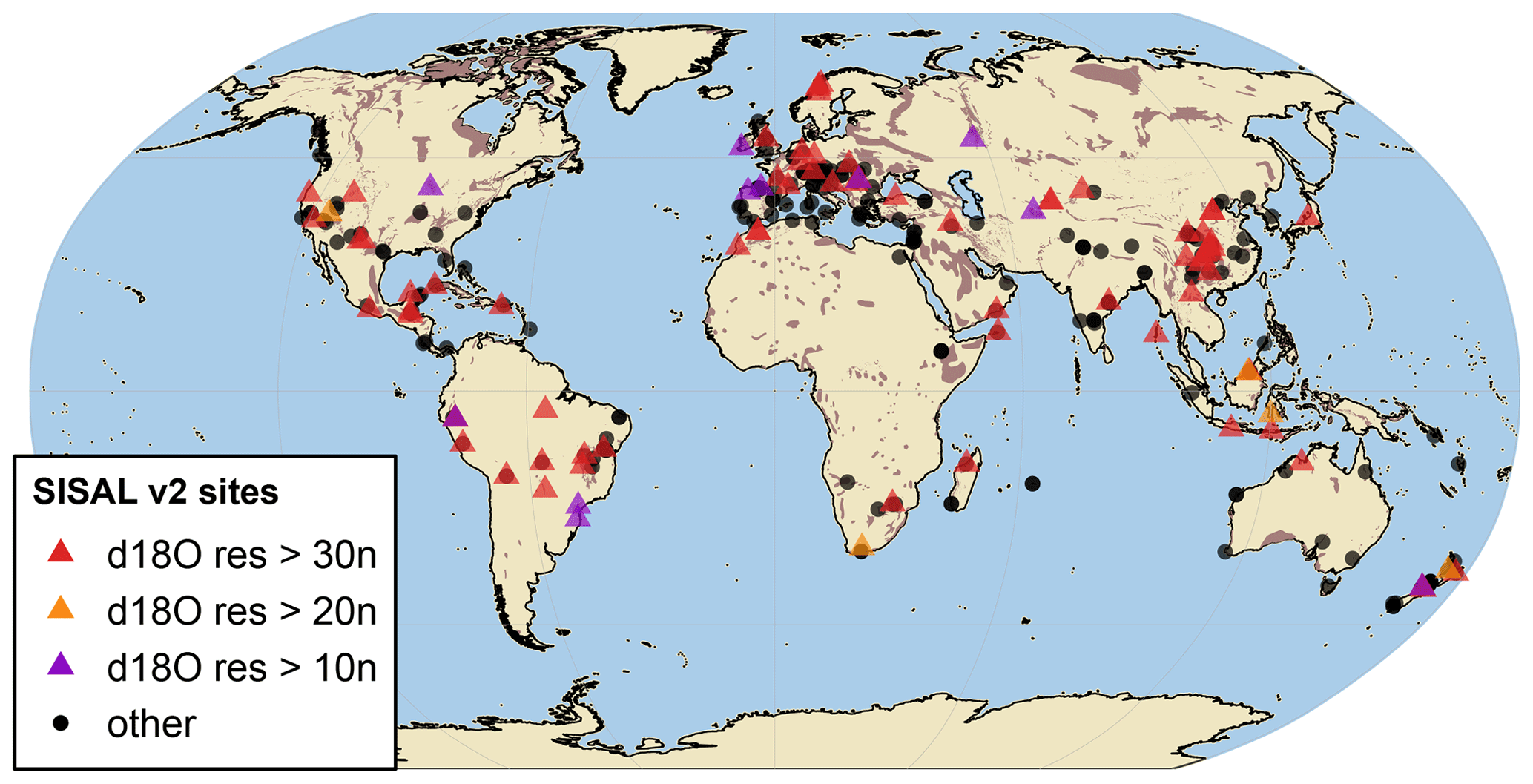
Figure 2Site locations of the SISAL database on a global karst map (brown shadings from Williams and Ford, 2006). The sites with entities that fulfill the prerequisites for our analysis are marked in colored triangles. These entities cover at least a period of 600 years within the last millennium and have a minimum of 30 (red), 20 (orange), or 10 (purple) δ18O measurements and two dating points in this period. All other sites in the SISAL database v.2 are marked with a black dot. The nine clusters used in the network analysis contain sites in North America (c1, 12 entities), South America (c2, 12 entities), Europe with northern Africa (c3, 21 entities), southern Africa (c4, 2 entities – too few for systematic analysis), the Middle East (c5, 6 entities), India and central Asia (c6, 8 entities), East Asia (c7, 18 entities), Southeast Asia (c8, 3 entities), and New Zealand (c9, 3 entities).
The Speleothem Isotopes Synthesis and Analysis is an international working group, collecting speleothem datasets in a quality-controlled and cross-referenced database with rich metadata for samples and dating procedures (Atsawawanunt et al., 2018; Comas-Bru et al., 2020b). The second version of the database SISAL v.2 includes measurements of stable 13C and 18O isotopes on speleothems of 691 individual entities from 294 globally distributed sites (Comas-Bru et al., 2020b). In order to provide a comprehensive and reliable analysis, we only use data from entities which are not superseded (entity_state = current) and that cover at least a 600-year period within the analysis period (850–1850 CE). Furthermore, records considered must have at least two radiometric dates, or one radiometric date (in the analysis period) and be marked as actively forming at the time of collection, or be lamina counted. We only check for dates that are marked as used, indicating that they are known to have been used in the original chronology in the database. Samples without sample or depth information are omitted. In the analysis, we filter the database adapted to the requirements of the different analyses, as depicted in Fig. 2. For the last millennium, we retain 110 records from 91 different sites with at least 10 isotopic measurements, which we used for the assessment of the mean δ18O offset, and 85 records from 71 sites with at least 30 isotope samples for the correlation and network analyses.
For each -dated speleothem, SISAL v.2 provides the original age model (if available), and new possible age models based on up to seven methods. Methods include linear interpolation, linear regression, Bchron (Haslett and Parnell, 2008) as adapted by Roesch and Rehfeld (2019), Bacon (Blaauw and Christeny, 2011), Oxcal (Ramsey, 2009), copRa (Comas-Bru et al., 2020b, modified R version after Breitenbach et al., 2012), and StalAge (Scholz and Hoffmann, 2011). Details on the automated age-modeling procedure are given in Roesch and Rehfeld (2019) and Comas-Bru et al. (2020b). For each entity and ensemble method, one median best-fit estimate with confidence intervals and between 129 and 7737 age models based on perturbations of the radiometric ages are available (Comas-Bru et al., 2020b). These ensembles are available for 69 of the 85 entities that we used in the network-correlation analysis, resulting in a total of 464 383 ensemble age models in our analysis. In all other analyses, we use the corresponding original age model as provided by the original authors.
3.1 Speleothem analysis and drip water conversion
To increase the robustness of the results, we maximize the number of records by adaptive filtering of the database (Fig. 2). For calculations involving the time-averaged δ18O values, we only use speleothem data with at least 10 δ18Ospeleo measurements and two dating points within a 600-year period in 850–1850 CE. For variance analyses, we demand at least 20 and for spectral, correlation, and network analyses 30 δ18Ospeleo measurements. For the investigation of spatial correlation patterns by network analysis, the set of speleothems is divided into nine regional clusters (Fig. 2), as explained in detail in Sect. 3.3. We primarily use the chronologies provided by the original authors but test for the sensitivity to age-modeling choice by considering the age-model ensembles (details below in Sect. 3.3).
Within the last millennium, we remain with 15 aragonite and 89 calcite speleothems with 10 or more δ18O samples. Following Comas-Bru et al. (2019), we exclude six speleothems of mixed mineralogy, as the extent to which the applied conversion is appropriate is unclear. The δ18Ospeleo signal of calcite and aragonite speleothems is converted to its drip-water equivalent (δ18Odw.eq) relative to the V-SMOW standard as in Comas-Bru et al. (2019). For calcite, we use the empirically based fractionation formula of Tremaine et al. (2011).
where T is in K and δ18O in units of ‰. For aragonite, we use the fractionation factor from Grossman and Ku (1986):
Here, temperature values T represent the local cave temperature in units of K. These are often not available. The annual mean temperature on the surface above the cave can, however, serve as a surrogate for local cave air temperatures (Fairchild and Baker, 2012). For both aragonite and calcite drip water conversion, we use the simulated annual mean temperatures at the cave location, down-sampled to the temporal resolution of the record. Note that, as a consequence, the conversion changes the time-averaged mean and the variance in our analysis. Finally, the V-PDB to V-SMOW conversion from Coplen et al. (1983) is used.
Whenever we directly compare simulation output values with the speleothem records, e.g., when comparing means, variances, or spectra, we use δ18Odw.eq, accounting for the different mineralogies. The conversion would, however, add an extra source of uncertainty in correlation analyses, as it implicitly builds on transient simulation data. Therefore, we denote the raw values of δ18O measured directly in the calcite or aragonite matrix by δ18Ospeleo and focus on those in the network and correlation analyses.
3.2 Statistical tests and time series processing
Speleothems form naturally and therefore provide irregular time series with reconstructed and uncertain observation time series (Rehfeld and Kurths, 2014). We account for this in our assessment as outlined below. Temperature, precipitation, and isotopic data are extracted from the simulation at cave locations by bi-linear interpolation. Annual mean values for temperature, precipitation, and isotopic composition of precipitation are formed by averaging over all months from April to March of the following year. This is also the time span for which precipitation-weighted δ18O (δ18Opw) values are calculated, all for each simulation individually. This allows the dynamic response in the signal to be examined. All analyses are conducted using both simulated δ18O and δ18Opw. Differences in mean are given in (model–data difference) and variance ratios in the record's variance divided by the variance of the simulation at the cave location (). If not explicitly stated otherwise, we always provide 90 % confidence intervals by bootstrapping (Efron and Tibshirani, 1986) with 1000 repetitions. To reduce potential bias due to the irregular spatial distribution of cave sites, we use area-weighting in spatial mean estimates, where stated. This is done by calculating grid-box means of all speleothems within a 3.75∘ × 2.5∘ grid box similar to the simulation, which is then area-weighted across latitudes, following Marcott et al. (2013).
While the simulation data are available on a monthly basis, the proxy time series are irregular and at annual or lower resolution. Therefore, the simulation data at cave location are down-sampled to the record's reconstructed time axis by block averaging. The power spectral density (PSD) of a time series over a finite interval of time describes the distribution of power in frequency components of the time series. The integration over all spectral components yields the variance of the time series (Chatfield, 2003). For spectral analyses, the proxy records are interpolated to their mean resolution in a double interpolation and filtering procedure (following Laepple and Huybers, 2014a, b; Rehfeld et al., 2018; Dolman et al., 2020). Spectra of sufficient resolution can then be averaged to a mean spectrum over a certain frequency range (Kunz et al., 2020).
We test the impact of karst storage of drip water (Gelhar and Wilson, 1974; Dee et al., 2015) by applying an additional simplified aquifer recharge-model-style filter (hereafter karst filter). The impulse response of the Green's function depends solely on the transit time τ, as , with t>0. The Green's function is convolved with the simulated input δ18O or signal to obtain the simulated karst-filtered signal in the cave. Following Dee et al. (2015) we use a normalization such that , integrated over the length of the respective time series. For the down-sampled case, we first apply the filter to the annual-resolution simulated δ18O and down-sample to record resolution afterward.
The correlation of irregular time series is estimated by Person correlation adapted for irregular time series (Rehfeld et al., 2011; Rehfeld and Kurths, 2014). The signal-to-noise ratio (SNR) is estimated from the estimated cross-correlation between two time series i and j by calculating , as described by Fisher et al. (1985). If more than two estimates are available, e.g., at the grid-box level, the median between all possible combinations of cross-correlations between the time series is used.
For correlation estimation, we choose a significance level of α=0.1. In balancing the strictness and the expected level of false positives against that of data demands and the available number of samples N, the level is appropriate for both paleoclimate archive and model data time series. The p values for irregular series are estimated based on a t distribution, with the degrees of freedom estimated from the temporal coverages Rx,y and the persistence time τx,y as . This is implemented in the R package nest (https://github.com/krehfeld/nest, last access: 29 April 2021, Rehfeld et al., 2011; Rehfeld and Kurths, 2014). In the case of the speleothem records, the estimated effective degrees of freedom range from Neff=20 to Neff=470, and they are generally similar to the length of the records. For the regular time series, p values are calculated via Pearson's product moment correlation (via the function cor.test).
We account for age-model sensitivity by calculating cross-correlation estimates for all possible combinations of available age-model ensembles (Comas-Bru et al., 2020b). The provided age models are not a priori ranked by likelihood and are all consistent with the radiometric chronological constraints. The age-model pair that results in the strongest significant absolute correlation estimate (p<0.1) between two records is selected for the best selection tuning.
3.3 Spatial correlation via network analysis
Networks are practical representations for complex systems with interacting components and can be used to analyze dynamics in the climate system (Tsonis et al., 2006; Tupikina et al., 2014; Rehfeld et al., 2013). Here we use a network with n nodes, where n is the number of SISAL v.2 entities that fulfill the sampling criteria. The speleothem entities are joined in pairs by edges or links, where the links are formed if the cross-correlations between two speleothem entities i and j are significantly different from zero with a p value of pi,j.
We split the network into eight sub-networks by hierarchical distance-based clustering of the node locations. The cluster that includes all East Asian caves is manually split into two clusters, one for East Asia (all caves above 20∘ N) and a cluster for Southeast Asia (all caves below 20∘ N). With this, we end up with nine clusters as depicted in Fig. 2. Links in the plots (Fig. 8) are visualized if they are stronger than a certain threshold , where r5 % is the minimum correlation strength of the 5 % absolute strongest correlations (“fixed link density”).
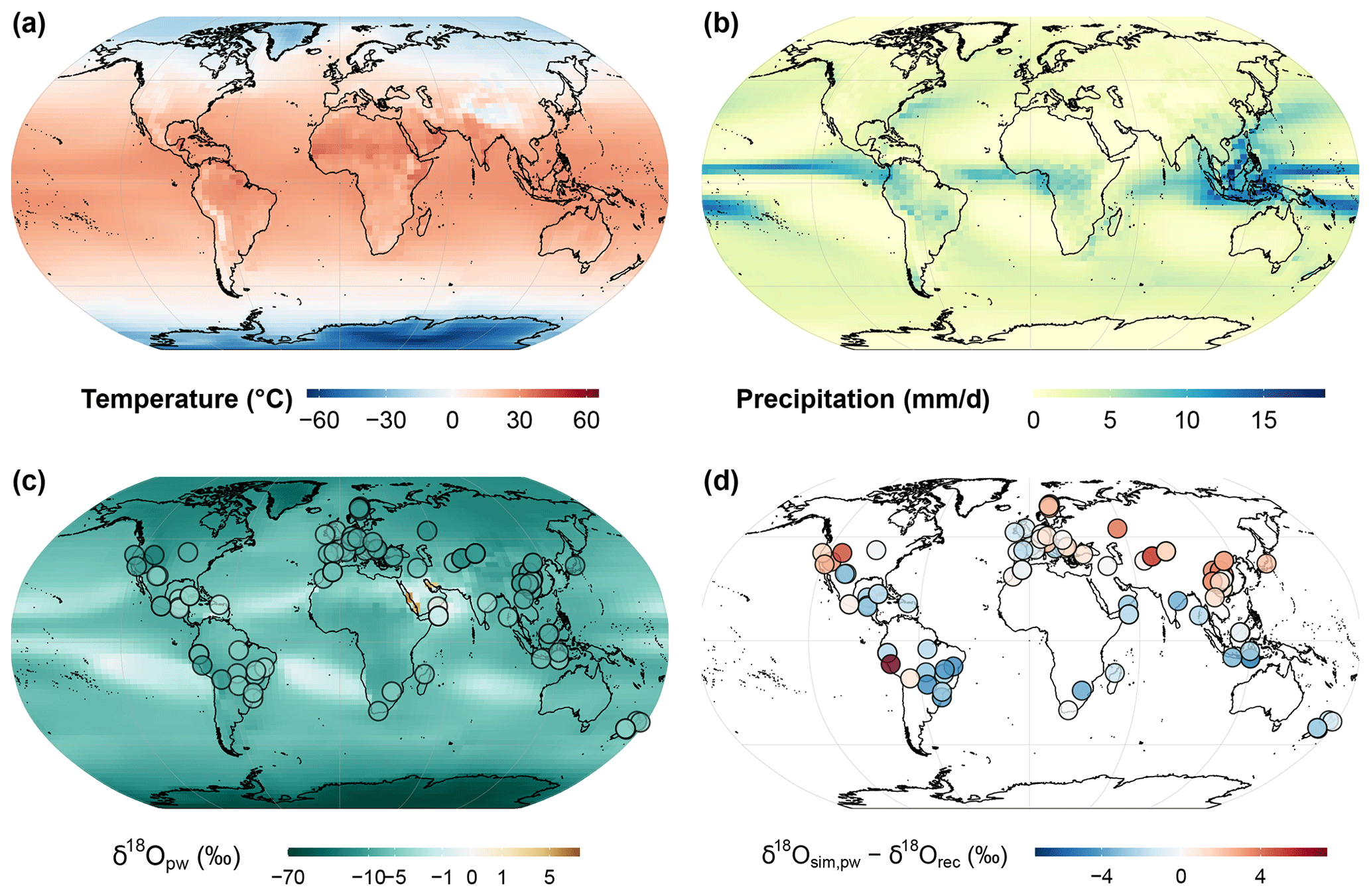
Figure 3Characterization of the mean state of the simulation (LM1): shown are (a) mean annual surface temperature, (b) precipitation, and (c) , including δ18Odw.eq at cave sites in drip water equivalents. Note the logarithmic color scale. Point-wise differences between the mean simulated δ18O and proxy-based δ18Odw.eq (d) show anomalies. Spatially aggregated differences at the global and cluster level for simulations LM1–LM3 are given in Table S1 in the Supplement.
4.1 Assessing model–data differences in time-averaged δ18O
We first compare the mean SISAL v.2 record δ18Odw.eq and iHadCM3 δ18Opw to assess potential model biases, using the 104 records with more than 10 δ18Ospeleo measurements within the last millennium. Annual mean temperature and precipitation fields (Fig. 3a, b) and the mean modeled δ18Opw together with the mean δ18Odw.eq in the SISAL records (Fig. 3c) are shown in Fig. 3. Shown and described are the fields and results for LM1; results for the other ensemble members are generally very similar and given in Table S1 in the Supplement. The major oxygen isotope ratio depletion features as described by Dansgaard (1964) can be distinguished. Modeled values show progressive depletion towards higher latitudes, the interior of continents, and towards regions with high precipitation amounts.
The offsets between modeled and measured δ18Opw () show a heterogeneous pattern (Fig. 3d). Generally, modeled values appear to be more depleted overall than the mean values of speleothem δ18Odw.eq, except in the Northern Hemisphere extratropics. There are some localized clusters and individual sites with large positive and negative differences. One example is site 38 (eID = 113, Diva cave in Brazil), which is visible as a dark blue dot in Fig. 3d. The δ18Odw.eq record shows only slightly depleted δ18O in calcite (), while the simulation shows much more depletion (). This results in a model–data difference of . The surrounding sites in Brazil are also less depleted than in the simulation. Site 277 (eID = 598, Huagapo cave in Peru), visible as a dark red dot in Fig. 3d, shows a strong depletion in calcite () while the simulation is not as strongly depleted (). This results in a large positive offset of Δδ18O=7.33 ‰. The cave is located at an altitude of 3850 m above sea level, whereas model altitude at the grid box is close to sea level. This should explain part of the offset.
At the regional scale, the largest cluster offset can be seen over China and East Asia (c7) (−0.18 ‰, 4.65 ‰, 90 % confidence interval). However, the most consistent negative difference is visible over neighboring Indonesia (c8) ). The smallest differences are found in Europe with (). Overall, the simulated δ18O is smaller than the δ18Odw.eq measured in speleothems ( ). The grid-box-level area-weighted global mean difference is for LM1.
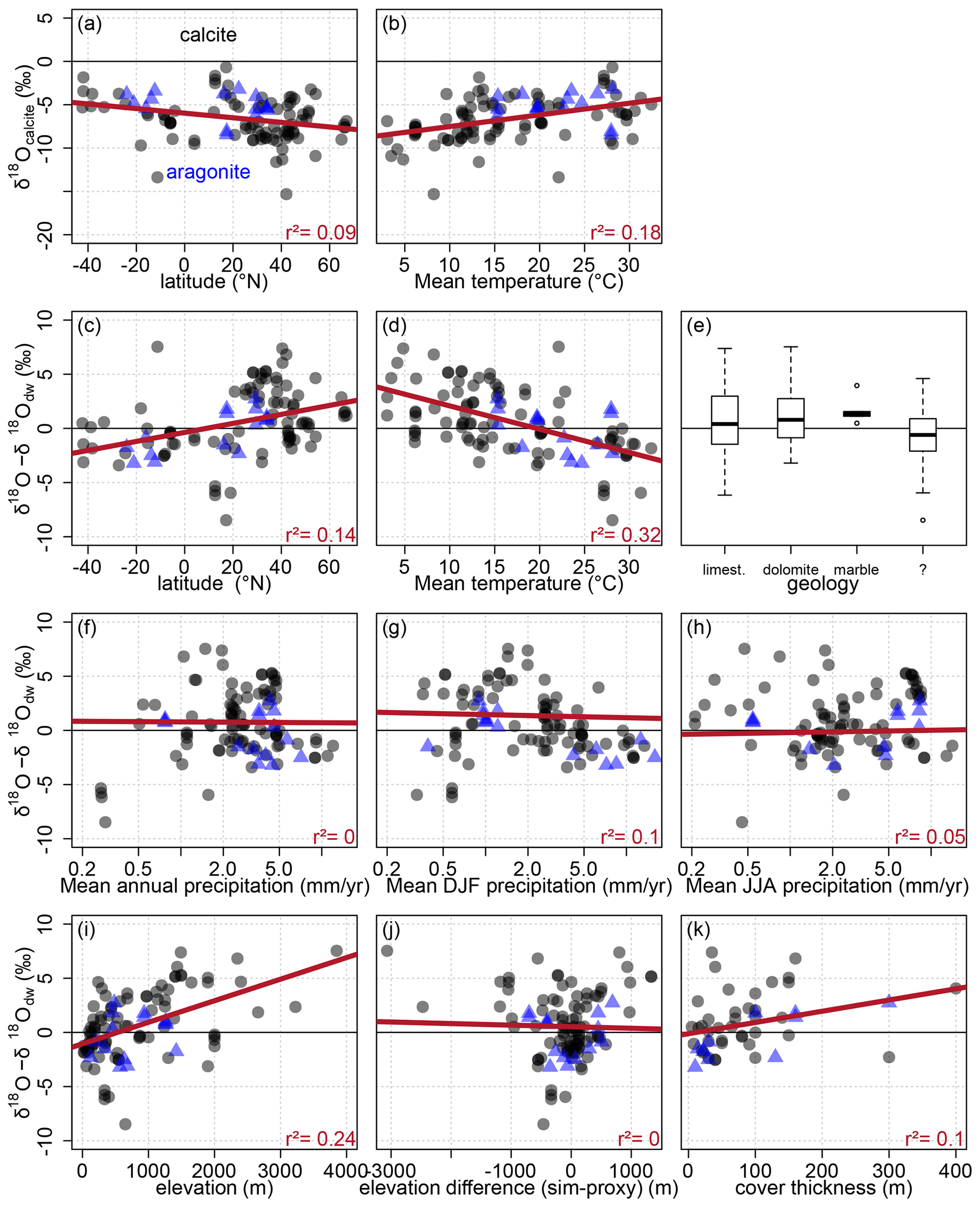
Figure 4Systematic comparison of climate variables from LM1 and cave parameters on δ18Odw.eq and the offset Δδ18O to the simulation. Shown are the absolute values of δ18Odw.eq vs. (a) site latitude and (b) simulated local annual mean temperature, and the model–data difference vs. (c) latitude, (d) simulated mean annual temperature, (e) geology surrounding the cave (“?” means unknown geology), and (f) mean annual precipitation amount from (g) DJF and (h) JJA as well as (i) cave elevation, (j) the elevation difference between the model grid and actual cave, and (k) the overall cover thickness above the cave. Symbols denote calcite (black circles) or aragonite (blue triangles) specimens. An unweighted linear regression (red line) is added for illustration, but without consideration of significance.
We further explore the impact of site conditions on the model–data offset (Fig. 4). We find a decreasing δ18Odw.eq towards northern higher latitudes (Fig. 4a), and most notably a dependency of δ18Odw.eq on the local mean annual temperature (Fig. 4b). We see more positive offsets in the Northern Hemisphere and mostly negative offsets in the Southern Hemisphere (Fig. 4c) as was also distinguishable in the map in Fig. 3d.
The offsets also show a strong influence of temperature (Fig. 4d) and elevation (Fig. 4i), which are both controlling factors during the isotopic fractionation process. The elevation difference between the simulation and the record spans from a 1332 m higher elevation in the simulation (eID = 538 in Shenqi cave in China) and 3065 m higher elevation in the records (eID = 598 in Huagapo cave in Peru, visible outlier in Fig. 4c, d). Here, the offsets increase with increasing absolute difference (Fig. 4j). The offset shows a weak correlation with precipitation (Fig. 4f), both in the annual mean and for the boreal winter and summer seasons (see DJF and JJA precipitation in Fig. 4g, h). No relation can be seen with mineralogy, parent rock (Fig. 4e), or cover thickness (Fig. 4k).
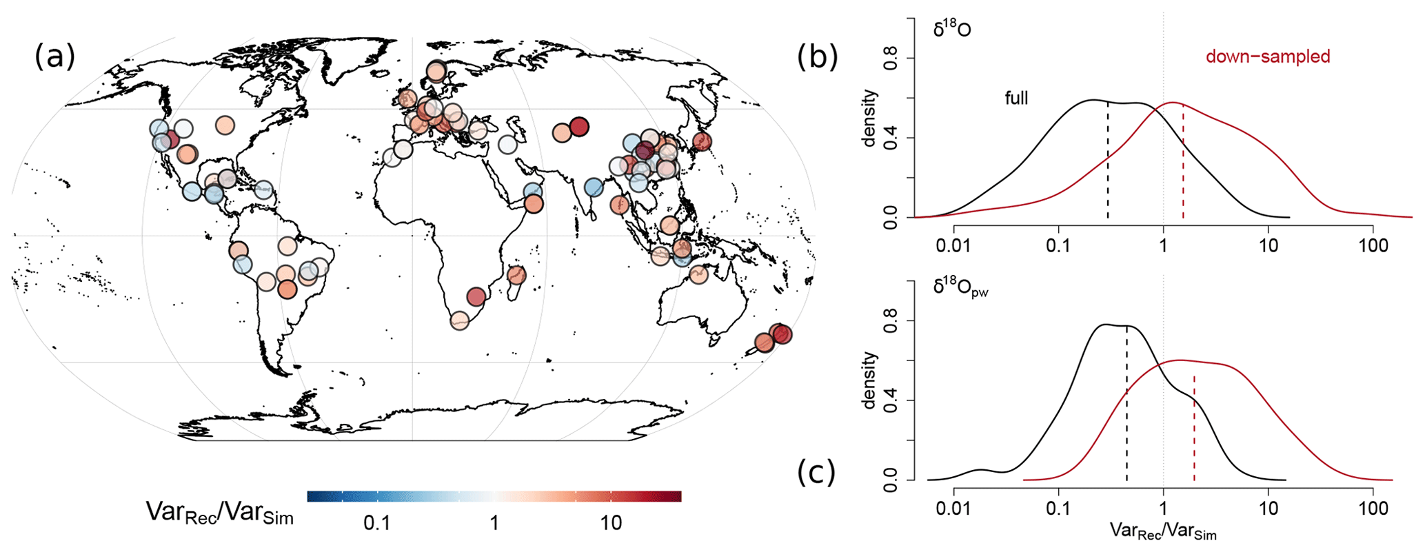
Figure 5(a) Spatial visualization of the site-based dimensionless variance ratio , where the simulated δ18O is down-sampled to record resolution, based on LM1. Aggregated density plots of the variance ratio of δ18O (b) and precipitation-weighted δ18Opw (c) for the raw records (“full”, black lines). The simulation has also been down-sampled to the record resolution (“down-sampled”, red lines), which illustrates the variance loss due to temporal averaging in the archive (uses LM1-3).
4.2 Assessing model–data differences in the local variance of δ18O
To analyze how similar the variability of the isotopic signal is in the iHadCM3 climate model and the speleothems, we compare the total variance of the simulation to that of the 92 speleothem records with more than 20 δ18Ospeleo measurements over the last millennium. The global distribution of variance ratios between δ18Odw.eq and down-sampled δ18O (Fig. 5a) shows overall higher variability in the speleothem records than in the simulation, with local exceptions. This is also corroborated by the density plots of the ratio for both δ18O and in Fig. 5b, c. Generally, the observed proxy variance is roughly 2 times higher than that of the down-sampled simulation δ18Opw at the cave location (median of the histogram at 1.8 (1.4,2.6) in Fig. 5b, c). This is consistent with the predominance of red-shaded variance ratio visualizations in the spatial view indicating (Fig. 5a). However, there is a clear impact of averaging on the total variance, as down-sampling results in a variance ratio above unity. Overall, this shows a discrepancy between the variance observed in δ18Odw.eq and the simulated variance at the cave location over the total time period.
The highest variance ratio for down-sampled δ18Opw is found in Jiuxian cave in China (eID 330, with a variance ratio of 49.5) and the lowest variance ratio in Dandak cave in India (eID 130, with a variance ratio of 0.2), while neighboring caves show very different variance ratios. As the modeled patterns are fairly smooth, this indicates a large heterogeneity of the speleothem data from the cave environment. We find no strong or significant relationship between variance or variance ratios to any tested climate or cave parameter (Fig. S4 in the Supplement where we show a similar figure to Fig. 4 but for variance ratios).
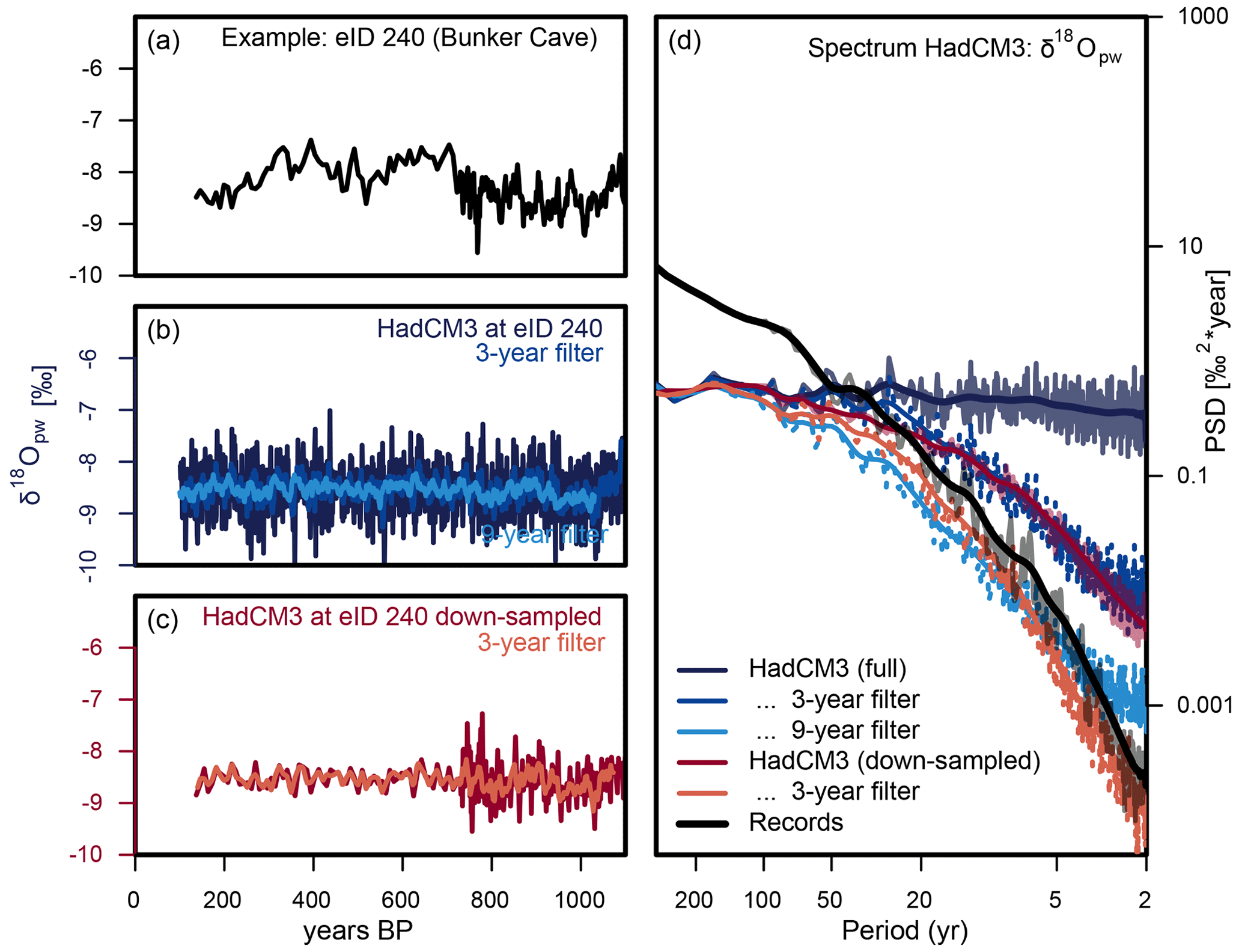
Figure 6Variability on different timescales through comparison of measured δ18Odw.eq and simulated δ18Opw time series as well as of their spectra. (a–c) Example time series of eID 240 in Bunker cave (Germany) (Fohlmeister et al., 2012). (a) The measured δ18Odw.eq in the speleothem, (b) the iHadCM3 simulated δ18Opw at the cave location with two filters (3 and 9 years), and (c) the simulated δ18Opw but down-sampled to the same temporal resolution as in (a) with a 3-year filter. (d) Power spectral density (PSD) of mean spectra of simulated δ18Opw at the cave site in yearly resolution (blue), down-sampled to the individual record's resolution (red), and mean spectrum of the δ18Odw.eq of the records (black), including the karst filter as shown in (a)–(c). The spectra are area-weighted and averaged over the three simulations (LM1, LM2, and LM3). The colors for the example eID in (a)–(c) correspond to the colors of the mean spectra over all entities in (d).
4.3 Assessing δ18O variability at interannual to centennial timescales
We extend the analysis of total variance (Fig. 5) to the timescale-dependent variance (Fig. 6) to better explore variability on interannual, decadal, and centennial timescales as compared to the total variance over the last millennium. We set stronger criteria on the speleothem records and only analyze the 85 with more than 30 measurements over the last millennium. The spectra in Fig. 6d give an insight into the variability over different timescales and the representativity of records for reconstruction resolution.
On the left side (Fig. 6a–c), the time series of δ18Odw.eq of eID 240 (Bunker cave, Germany) is depicted (Fig. 6a), together with the simulated δ18Opw at the cave site at different temporal resolutions (Fig. 6b, c), including karst-filtered δ18Opw. Comparing Fig. 6a–c visually, different levels of variance can already be distinguished, for example, between the filtered and unfiltered simulated data. The iHadCM3 δ18Opw spectrum of the yearly resolved signal has similar variance over all frequencies and shows a fairly constant PSD (Fig. 6d). Variance at decadal timescales (i.e., the PSD for higher frequencies) is just as high as the variance on centennial timescales (i.e., the PSD for lower frequencies).
After down-sampling to the irregular resolution of the record, the simulated spectrum loses power in the higher frequency range. Comparing for example the time series in Fig. 6c to the spectra in Fig. 6d, the down-sampled spectrum indicates lower variability than the annual resolution spectrum on decadal timescales. On centennial timescales, both spectra display similar variability. Contrasting Fig. 6b to c, this loss in decadal timescale variability is also visible on the time series level.
The proxies' spectra have even fewer frequency components in the high frequency range, due to the lower temporal resolution. They do, however, show a higher PSD at lower frequencies. The records are, therefore, less variable on decadal timescales, and more variable than both the down-sampled and the full-resolution simulated δ18Opw on centennial timescales.
An additional impact of karst processes and storage on the δ18Opw variability could be expected. To test the impact of this, we apply simple karst filters (see Sect. 3) with increasing filter length and test whether they reduce the spectral mismatch. Filters of different lengths resulted in increasing spectral slopes with increasing transit times. A 3-year filter for the down-sampled δ18Opw achieves equivalent variance trends as the record spectrum with less power on decadal timescales. It eventually flattens again for longer timescales, without exceeding the PSD of the unfiltered signal, such that it is less variable than the proxies on longer timescales. A full set of individual spectra (full simulation, down-sampled, record spectrum, and all filters) for all entities used in this analysis can be found in Figs. S5 and S6.
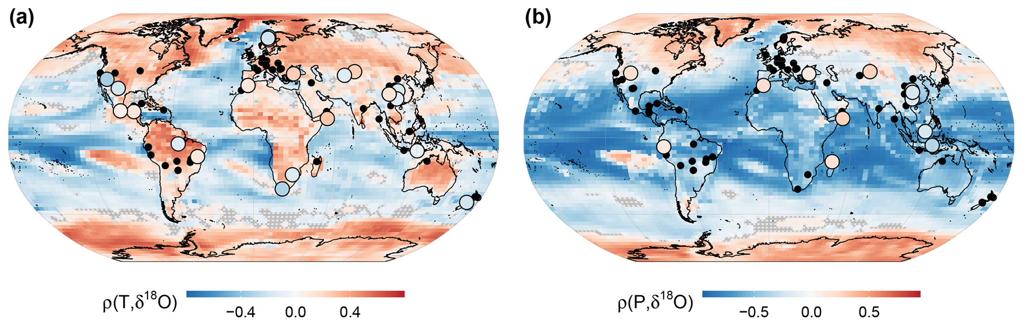
Figure 7Correlation fields of simulated δ18Opw and the related climate variables surface temperature (a) and precipitation (b) for simulation LM1 (). Colored symbols give the correlation between simulated climate variables and the δ18Odw.eq of the speleothem records. Empty tiles mask non-significant correlations. Black dots show cave locations with non-significant correlations.
4.4 Climatic drivers of δ18O variability
To distinguish the main important climatic drivers for specific areas for δ18O both in the simulation and in speleothems, we correlate simulated δ18Opw with the simulated temperature (Fig. 7a) and the precipitation signal (Fig. 7b) on a grid-box level after temporal down-sampling. Grey (empty) tiles indicate non-significant correlation estimates. The correlation between δ18Ospeleo and the climate variable is also shown.
We see strong correlations of simulated δ18Opw to simulated temperature at high latitudes as well as over some landmasses (background in Fig. 7). The speleothem signals show positive as well as strong negative correlations. The absolute highest correlation is found for eID 124 in Leviathan cave in the USA (). In the simulation, this correlation is locally positive, which indicates that the simulated temperature is a positive δ18Opw driver in the general area in the model. The correlation of the simulated climate and the record's δ18Ospeleo is, however, negative.
The correlation between the simulated precipitation and δ18Opw is especially strong in the tropics. We find the highest absolute correlation for eID 523 in Gempa Bumi cave in Indonesia (). Here, the background also shows a negative correlation.
Comparing the two proposed climatic drivers of δ18Opw variability, we observe that the correlations to temperature are higher in the higher latitudes, while correlations to the precipitation appear more important in the tropics. A fairly clear zonal structure of correlations between the climate and oxygen isotope ratio fields is visible in the model. However, only a few of the records show a significant correlation (p<0.1). We find 18, 15, and 22 significant correlations from 85 entities for temperature for the 3 LM ensemble runs respectively. A total of 44 of these are from entities that show significance in 2 of the 3 LM runs. For precipitation, we find 14, 7, and 10 significant correlations where 54 entities are significant in at least 2 of the 3 LM runs. No clear climatic driver can, therefore, be extracted alone from record correlation results. Fewer records show significant correlation to both climate variables. The direct correlation of the time series of the simulated and proxy-based δ18O results in only 19, 17, and 19 significant correlations from 85, i.e., at around 20 % of the sites. Here, 45 entities show significant correlations in 2 or 3 of the LM runs.
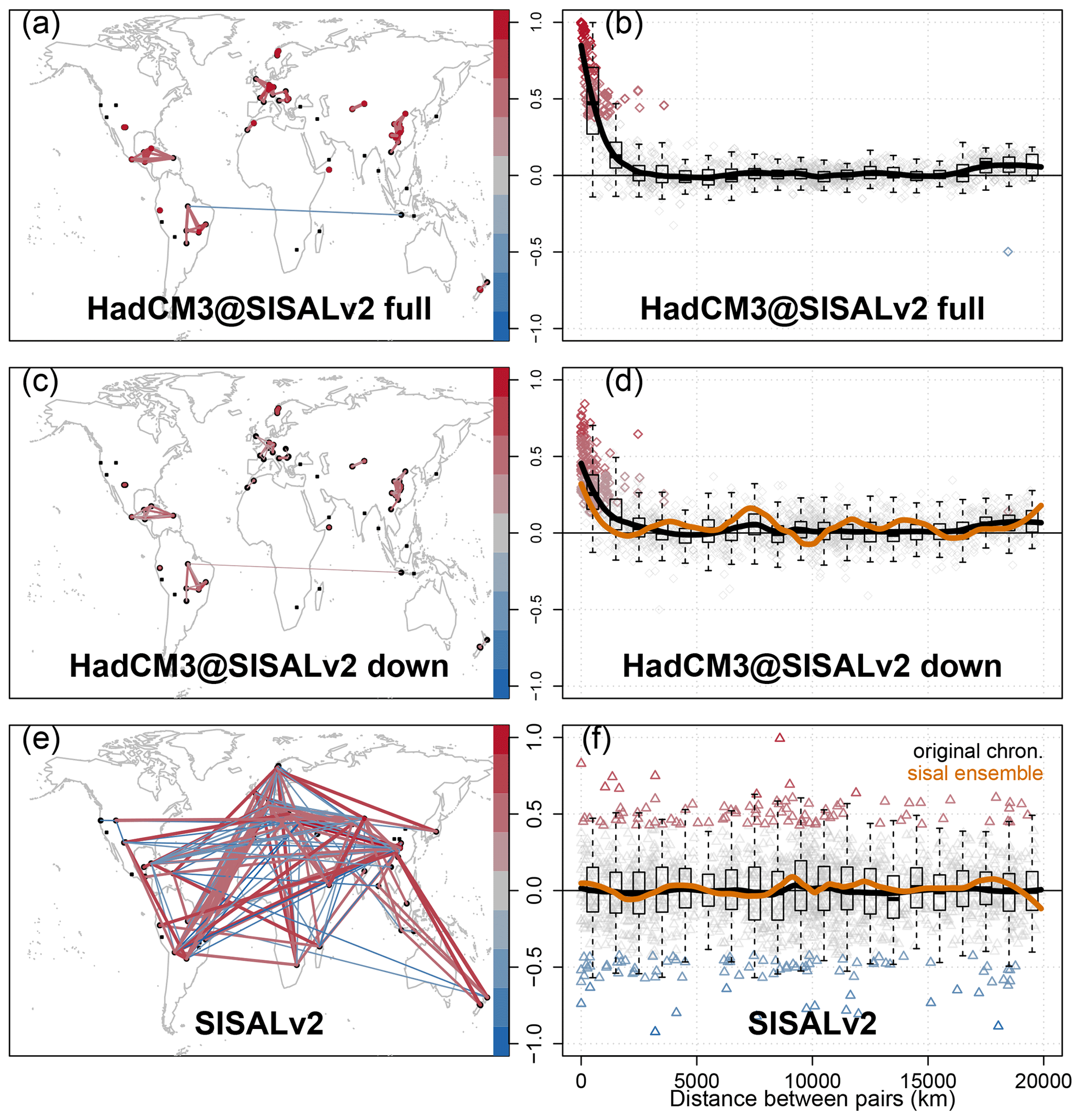
Figure 8Network spanned by the 5 % strongest absolute correlations of simulated iHadCM3 LM1 δ18Opw at the SISAL cave sites: (a) full (i.e., annual) resolution, (c) down-sampled. All model-based between-site correlations are shown in the distance-binned boxplot (b, d). Network visualizations (e) and distance-binned boxplot (f) of the cross-correlations between SISAL site δ18Ospeleo for the original age models. The color values indicate the 5 % strongest correlations in network and boxplot. The LOESS smoother (span = 0.2) in the boxplots indicates the correlation for the original chronology (black) as well as the absolute highest correlation through selection of age models (orange).
4.5 Similarity measures and network analysis
Computing all statistical similarity between the δ18Ospeleo signals within a cave (“site-level correlation”) or across nearby caves (regional or grid-box-level correlation) yields a measure of representativity useful for model comparison and uncertainty assessment. The networks in Fig. 8 are based on the simulated signal (annual resolution and down-sampled) δ18Opw (Fig. 8a–d) and for δ18Ospeleo (Fig. 8e, f) for 85 entities.
Network links are based on the 5 % highest absolute correlations. The highest correlations are found at close proximity for the models (Fig. 8a–d), whereas links across a wide range of distance can be seen in the proxy data (Fig. 8e, f). High local correlations for the model data can be expected, as the simulated δ18Opw within one cave will be the same and only differs on a temporal scale after the adjustment to the entity's temporal resolution (down-sampling). The mean absolute correlation for the 5 % strongest significant links in Fig. 8c) is . Comparing the down-sampled distance-to-correlation plot (Fig. 8d) to that on annual resolution analysis (Fig. 8b), an additional scattering of correlation estimates at longer than 2000 km distance is visible.
The network of δ18Ospeleo does not display large-scale spatial patterns and no observable relationship between correlation and distance. The mean absolute correlation for the 5 % strongest significant links shown in Fig. 8e is . Computing the networks based on the ensemble age models, as well as selecting the age models that maximize the absolute correlation between sites, amplifies both positive and negative correlation estimates but does not change the correlation-to-distance relationship. The sensitivity test performed on the simulated down-sampled δ18Opw still shows strong yet weaker correlation estimates at short distances. Comparing the results for simulated δ18Opw (Fig. 8a–d) and δ18Ospeleo (Fig. 8e, f), we obtain low correlation estimates at the local scale.
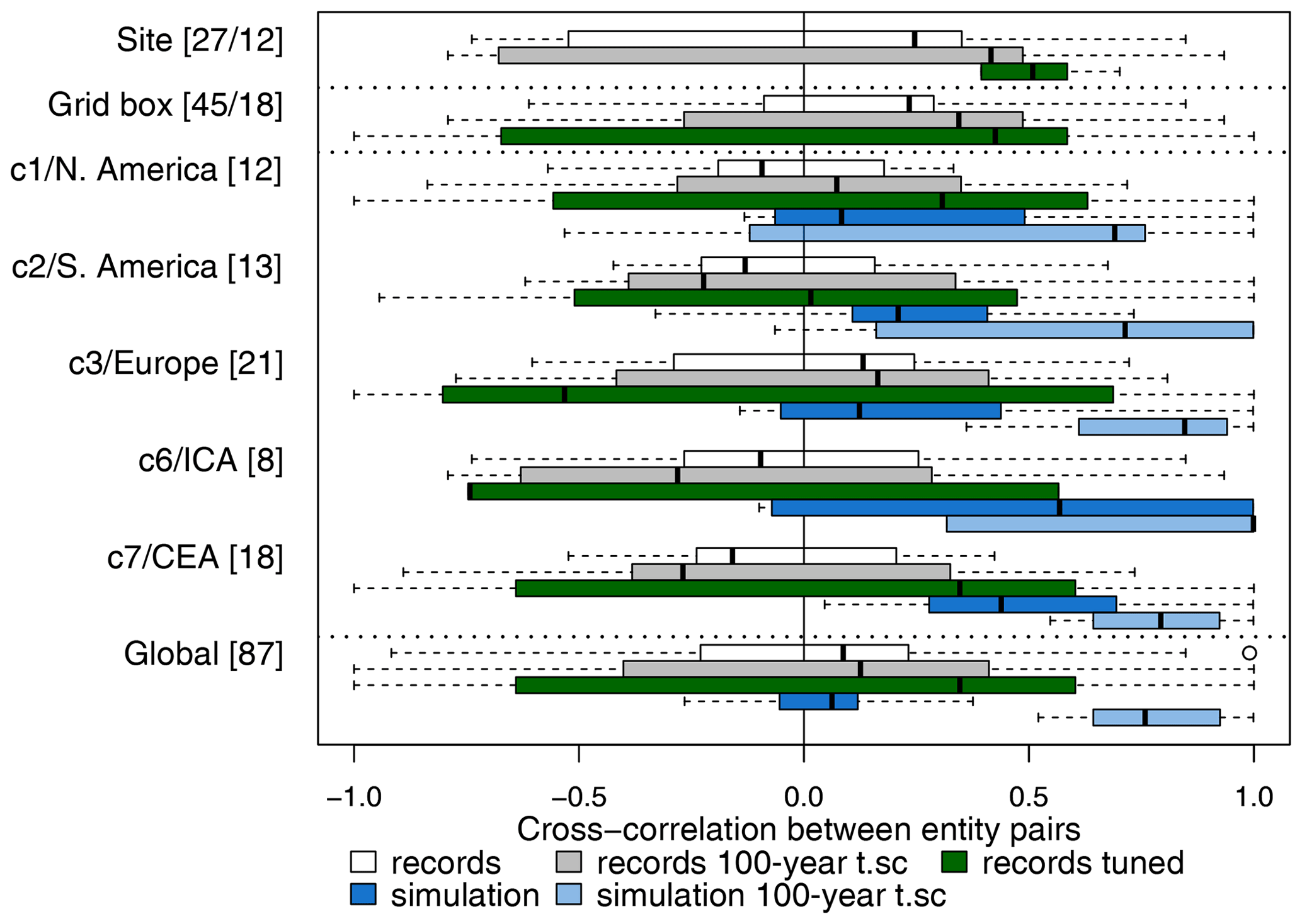
Figure 9Cross-correlation on site, grid boxes, clusters and global scale for speleothem records and the locally interpolated model output for δ18Opw. The 12 (18) sites (grid boxes) contain more than one speleothem entity with a total of 27 (45). At each aggregation level the correlation estimates between all entities is shown for δ18Ospeleo (white bars), and the down-sampled model output δ18Opw of LM1-3 at cave locations (blue bars). Different temporal scales (original resolution and 100-year timescale (t.sc)) are compared as well as the age-model ensemble that gives the highest absolute correlation (dark green bars). Clusters are indicated with the number of speleothem entities in brackets, where c4, c5, c8, and c9 are not included because they contain too few entities. c6/ICA is the India and Central Asia cluster, c7/CEA is the China and Eastern Asia cluster.
We can also investigate relationships using regional networks. For this, we look at correlation on different spatial levels and separate the network analysis from Fig. 8 by sites, grid boxes, and clusters. Cluster c4, c8, and c9 contain less than four entities and are excluded. We check for representativity on different timescales of record resolution (white and dark blue) and a 100-year Gaussian smoothing filter (grey and light blue) and on different spatial scales using boxplots (Fig. 9).
At the site level, we find 27 entities within 12 sites that contain at least 2 entities. The median correlation of these 28 pairs is . On a 100-year timescale, this increases to ). The SNR gives a measure of the relative importance of non-climatic overprints on the proxy signal. We obtain a local SNR estimate of 0.5 (0.4,1.1). On the grid-box level (45 entities in 18 grid boxes), we find a median correlation of (100-year timescale: ). As on spatial resolutions below grid-box level, correlations between simulated δ18Opw are not meaningful, which is why the analysis in Fig. 9 shows only the correlations between record δ18Ospeleo and not those of the simulated δ18Opw on a site and grid-box level.
For regional clusters, the correlation between proxies shows positive and negative median values. In the simulation, the median values are always positive. For clusters containing more than 10 records detailed correlation maps including correlation matrices are depicted for Europe (Fig. S7), China and Eastern Asia (Fig. S8), South America (Fig. S9), and North America (Fig. S10) where very red maps and matrices can be found, indicating mostly positive correlations for the down-sampled simulation when compared to more blue ones in the records, indicating that negative correlations are also present. On the global scale, the median correlation between all records is slightly positive (, 100-year timescale: ), whereas for the simulation this median is positive () and strongly enhanced at centennial timescale to .
By the selection of the age model that maximizes the absolute correlation, we obtain a significant positive correlation at site level and a stronger significantly positive correlation at grid-box level. A detailed table with median correlations and SNR using the original chronologies as well as using the described age-model selection on different spatial levels is shown in ST2. Calculating correlations for different age-model ensembles was only done for the 69 entities, where both age-model ensembles were available (-dated entities) in Comas-Bru et al. (2020b), and our strongest criteria were matched.
5.1 δ18O model–data comparison in mean and variance
In our study, we found the last-millennium mean iHadCM3-simulated δ18O to agree well with the mean state of the measured δ18Odw.eq (Fig. 3). The average unweighted offset of was small compared to the total δ18Opw and the area weighted standard deviation of of the global simulated mean δ18Opw. Measured δ18Odw.eq followed general isotopic signature patterns as described by Dansgaard (1964). The offsets are more positive in the extratropics of the Northern Hemisphere, which is also shown by their temperature dependency (Fig. 4).
Baker et al. (2019) distinguished between temperature zones of climatic controls on δ18O in offset analyses on drip water. They find a stronger influence of seasonality of precipitation in warmer climates, highlighting the importance of a karst-recharge model. Here, we also observed a strong temperature dependency reflected in the offset and δ18Odw.eq over the last millennium, showing the influence of fractionation and other internal cave processes on the δ18O in drip water (Fig. 4) but also additional fractionation processes of weighting through evaporation before the precipitated water enters the epikarst. The higher offsets on the Northern Hemisphere possibly indicate a stronger influence of the continental effect. Still, from the records alone and with no karst-recharge or evaporation information, we were not able to distinguish specific climatic control regions. This requires a more thorough analysis including monitoring data as well as more simulated variables.
We found no evidence that the variance ratio between record variance and simulated variance is related to the offset between simulation and records (Fig. S4 is similar to Fig. 4, with variance ratios instead of Δδ18O). Specifically, there is no correlation between site-level offset and site-level variance ratio (results not shown, , p=0.2). In general, the total variance of the simulated δ18Opw and of the speleothem isotopic signatures over the last millennium are consistent. Differences in variance can, to some extent, be attributed to the sample resolution of the records, whereas down-sampling of simulated δ18Opw decreases the variability on decadal timescales. The resolution to which the simulation is temporally aggregated impacts whether the variance in the simulation appears to be larger or smaller than in the records. The variance over the last millennium in the records is overall 1.8 (1.4,2.6) times as high as the simulated down-sampled variance in Fig. 5.
Furthermore, the simulated δ18O time series at the cave sites show less variability on centennial timescales than the time series of the records. This is true even when comparing the same temporal resolutions (timescale-dependent variance depicted in Fig. S11 for δ18Odw.eq, yearly-resolution δ18O, and down-sampled δ18O). This is in agreement with the findings of Laepple and Huybers (2014b), who compared simulated and reconstructed temperature variability across different timescales and found that the model–data discrepancies increased with timescale, particularly on a regional level.
If we assume that paleoclimate archives record climate variability correctly and that the proxy–climate relationships are not timescale-dependent or transient, discrepancies at the centennial timescale could in part be explained by the models' underestimation of variability, in particular on centennial timescales. However, we find little regional consistency and high heterogeneity in the variance estimates from the speleothem records. These findings point to the influence of karst and internal cave processes on meteoric δ18O or the impact of seasonally filtered data captured by speleothems, e.g., through strong evaporation in warm months, which is in agreement with McDermott et al. (2001). Age uncertainties that are not covered by the age-model ensembles could also be responsible for the low similarity between isotopic signals of neighboring speleothem entities.
5.2 Influence of the karst filter
By delaying the simulated down-sampled signal through a simplified karst filter with a transit time of 3 years, we obtained matching equivalent power spectra for the simulation and the records. Studies observing cave reaction time in karst systems find increases in drip rate after an increase in precipitation, e.g., after days (Riechelmann et al., 2011). More complex tritium measurements show actual transit times of years in the Bunker cave in Germany (Kluge et al., 2010), to decades in the Villars cave in France (Jean-Baptiste et al., 2019), depending on the karst hydrology. The karst filter effectively reduces the temporal resolution of the record beyond the nominal median of 5.6 years (Fig. 6). Such low-pass filtering to model drip water transit times has been used (Wackerbarth et al., 2010; Dee et al., 2015; Lohmann et al., 2013) to produce similar time lags of 2–10 years, indicating that the best-fit mean time lag for our karst filter of 3 years (down-sampled) is a realistic estimate for transit times.
We find low interannual to decadal variability in the δ18Ospeleo signals recorded by speleothems (Fig. 6). In part, this is likely due to the average resolution of the records, which lies close to these timescales. Furthermore, mixing processes in the soil and karst could play an important role, where soil δ18O is found to have much lower variability than precipitation δ18O (Tang and Feng, 2001).
On decadal timescales (shorter than 50 years), the karst filter reduced the resolution-adjusted variance by 34 % (20,43) and on longer timescales (longer than 50 years) by 4.0 % (3.3,4.4) of the non-filtered down-sampled variance. The total filtered and down-sampled variance over the last millennium decreased by 14 % (9,27) of the unfiltered down-sampled variance. Still, this is equivalent to only 29 % (23,38) of the record variance, as the filter only decreases variance on annual to decadal timescales. On centennial timescales the filter has little to no effect, so the record's variance on these timescales is not strongly affected.
5.3 Representativity of δ18O at different spatial levels
A clear picture of the relationship between the climatic drivers for the simulation was distinguishable. However, no systematic pattern and few significant correlations were found for the speleothem records (Fig. 7). Accounting for seasonal sensitivity could enhance the number of simulation-to-record correlations of Fig. S12, which shows the selected strongest seasonal correlation. However, this enhances neither the overall correlation (histogram of correlation distribution using annual down-sampled time series and seasonal down-sampled time series in Fig. S13) nor the SNR (results not shown). Still, the strong influence of seasonality suggests a dependency of δ18Ospeleo on certain seasons rather than the annual mean. Supporting this, Fig. S14 shows a correlation map with the strongest seasonal correlation of δ18Ospeleo to the simulated climate variables temperature, precipitation, and δ18O in precipitation. Further drip water monitoring studies combined with a comparison to model data output and observation data would help to characterize the seasonality of individual caves and would, therefore, lead to deeper understanding of which climatic signal is captured by speleothems and enhance comparability between different caves.
We found low spatial representativity of individual speleothems for sites, grid boxes, and regions when compared to the simulation (Figs. 8 and 9). We obtained stronger correlations between entities by selection of the best-matching age-model ensemble for entities where these ensembles were available. This age-model ensemble “tuning” increased the median of correlations on site and grid-box level by roughly a factor of 2, while also increasing the SNR by a factor of 3 and 2.5, respectively. However, no improvement could be observed on the cluster and global level. A detailed table of correlations and SNRs using the original chronologies as well as using the age-model ensemble selection that gives the highest absolute correlation is shown in Table S2 in the Supplement. Testing other “tuning” options, such as the consideration of only the 50 % of the records at closest proximity within a cluster or the 50 % with the smallest mean offset showed no improvement (boxplot similar to Fig. 9 for the other selection criteria in Fig. S15). We also found no correlation between the total variance and the number of significant links in the network (, p=0.8). Testing for age-model sensitivity and analyzing the resulting “tuning” for the down-sampled simulated δ18O in Fig. 8, however, yielded that the method is useful but better selection criteria are needed.
Examining climatic modes such as ENSO, NAO, and others (as shown in Fig. S18 for LM1), which modulate hydroclimate variability across spatiotemporal scales, may provide additional help in the interpretation of the climatic drivers, e.g., following the recent example of Midhun et al. (2021). They found that changes in modeled climatic mode strengths lead to small changes in δ18Ospeleo. The methods applied, especially regarding teleconnections, could provide deeper insight into climatic controls on speleothem isotopic signals. In particular Midhun et al. (2021) point out the potential to use of speleothem networks in the reconstruction of climatic modes.
A strong between-site variability has been attributed to controls of regional atmospheric circulation according to Lachniet (2009). We also find a strong heterogeneity in the recorded variance of δ18O at the grid-box and cluster levels. In part, this can be due to heterogeneous temporal resolution but could also be influenced by non-climatic environmental overprints on the δ18O signal up to the centennial scale. This could be investigated by comparing the δ18O and the δ13C signal recorded within the cave to vegetation, climate, and landscape evolution archives in the region. However, representativity tests across western Europe noted coherent δ18Ospeleo trends on glacial–interglacial timescales, where trends are less clearly expressed during the Holocene (Lechleitner et al., 2018). Therefore, this study could be extended to longer timescales, when longer transient isotope-enabled simulations become available.
5.4 Limitations
Simulated isotope variability is primarily dictated by the model's climatology and the complexity of its dynamics and hydrological cycle. We use a three-member initial-condition ensemble from a single iGCM in this study. Therefore, all results relate to these iHadCM3 last-millennium ensemble runs and the chosen radiative forcings. While solar forcing has little influence on simulated δ18O, the impact of volcanic forcing is much clearer yet still weak (Fig. S16). In this respect, a more thorough comparison with more simulations is needed in order to estimate the capability of models to simulate variability and to find common biases. However, the establishment of isotope-enabled GCMs requires substantial work for the addition of isotopic tracers and their evaluation, and the computational costs increase. This still inhibits the simulation of large transient ensembles with iGCMs over centennial to millennial and orbital timescales. Nevertheless, the three-member ensemble we provide could also be used to test offline data assimilation methods, as suggested by Dalaiden et al. (2020) or Sjolte et al. (2020). With their precise dating, speleothems are a well-suited archive for this method and age uncertainties can be accounted for similar to this study by the available age-model ensembles in Comas-Bru et al. (2020b). This might also help to better identify the climate factors that govern the speleothem archiving of δ18O and its variability.
An uncertainty factor in our study comes from the temperature dependence of the calcite- and aragonite-to-drip-water conversion. We calculated the adjustment factors using the simulated annual mean temperature at the cave location, sampled to the speleothem's temporal resolution. We take this simulated temperature as a surrogate for the long-term changes of the inside-cave air temperature. Knowing the actual temperature history of the caves better could strongly reduce the uncertainty, as a bias of Δ1 ∘C in the simulated temperature would account for a change in δ18Odw.eq of approximately Δ0.2 ‰. Following Eqs. (1)–(3), a bias of Δ1 ‰ in the δ18Odw.eq however, accounts for a temperature change of 4.5 ∘C for the lowest simulated annual mean cave temperature (3.1 ∘C in Norway), and a change of 5.5 ∘C for the highest simulated annual mean cave temperature (32.5 ∘C in the tropics).
This model–data comparison focuses on the comparison between simulated δ18O and precipitation-weighted δ18Opw to the drip-water-converted δ18Ospeleo. Especially in the more arid regions, evaporation processes play an important role, and δ18Ospeleo might be in better agreement with simulated infiltration-weighted δ18O or a karst recharge model. Further studies explicitly addressing evaporative effects might help in the interpretation of the results, for example in the region of South America.
Furthermore, our study focussed solely on δ18O as one particular proxy for climate and environmental changes and not other geochemical proxies that can be measured on speleothem samples (Kaufmann, 2003; Schwarcz et al., 1976) or a combination of proxies, which have the potential of a more thorough interpretation of a climate signal. A multi-proxy approach, such as in Fohlmeister et al. (2017) or Baker et al. (2017) who also include δ13C along with δ18O, could offer deeper insights. Many proxies for climate processes such as δ13C have not (yet) been implemented in comprehensive GCMs, as it requires a detailed and complex representation of the biology, physics, and ecology and dedicated model development. Therefore, in order to consider the vast majority of models in the evaluation, time series have to be calibrated to climatic and environmental parameters that are explicitly modeled. This would introduce additional uncertainty, which could counteract the added value of considering multiple proxies in the first place.
We have considered a regional to global view on speleothem δ18O signal. Therefore, influences and processes known for individual cave systems could not be considered. For example, Kluge et al. (2013) account for kinetic fractionation changes over time via clumped isotope measurements, and Jean-Baptiste et al. (2019) were able to extract transit times of drip water in Villar cave. Considering these and other local factors might give deeper insight into individual speleothem records, but it is difficult to scale quantitatively and systematically. Nevertheless, including monitoring datasets from different caves globally might give deeper insight into the filter and fractionation processes involved, and PSM studies informed by the monitoring and local expertise throughout the database could help in further comparison studies.
We presented an ensemble of iHadCM3 last-millennium simulations and compared the oxygen isotope ratios, temperature, and precipitation variability to oxygen isotope ratio observations from a large speleothem dataset (a subset of SISAL v.2). Overall, time-mean patterns of oxygen isotope ratio were fairly similar in both. Considering total variance as well as the variability on different timescales, we observed that the effects of resolution adjustment and a convolution karst filter were sufficient to bring simulated and observed δ18O spectra into good agreement. Still, total variability in the speleothem records is much higher than in the simulation. This supports previous studies that found that climate models currently do not capture appropriate variability on centennial timescales.
However, we find that the climatological and environmental interpretation of δ18Ospeleo is not straightforward. We found low signal-to-noise ratios for the isotopic signatures in the speleothem records, which imply a low spatial representativity of individual entities. Furthermore, while regional climatic signals were distinguished in the simulation, the main climatic drivers for δ18Ospeleo at the regional scale were difficult to isolate. It is difficult to establish the size of the spatial footprint of representativity, the seasonality, and the relevant climatological and environmental parameters for reconstructions. Here, expert knowledge on local cave processes, environmental history, and, in particular, the availability of monitoring data are crucial to aid the interpretation of the climate signal. Inner cave and karst processes, which influence the seasonality of the input signal above the cave and inside the cave, may need to be taken into consideration. However, monitoring data for evaluation and potential calibration of reconstructions are currently only available for a few sites (e.g., Tremaine et al., 2011). Furthermore, some parameters, such as transit times, are difficult to measure (Jean-Baptiste et al., 2019).
Proxy system models that account for the internal cave fractionation processes may give a deeper insight into how climate variability is captured in speleothem archives. To gain a deeper understanding of the underlying concepts that influence the capability of speleothems to capture and resolve climate variability and the capability of models to simulate them, further model–data comparison studies are required.
Code to reproduce figures and analyses in this paper are provided at https://github.com/paleovar/iHadCM3LastMill (last access: 19 February 2021, Bühler and Rehfeld, 2020). Model data are freely available on Pangaea at https://doi.org/10.1594/PANGAEA.924795 (Rehfeld et al., 2021) and Zenodo https://doi.org/10.5281/zenodo.4551065 (Rehfeld and Bühler, 2021). The SISAL v.2 database (Comas-Bru et al., 2020b) can be downloaded at https://researchdata.reading.ac.uk/256/ (last access: 29 April 2021, Comas-Bru et al., 2020a). We use R for the data analysis (R Core Team, 2020). The main packages are tidyverse (Wickham et al., 2019), ncdf4 (Pierce, 2019), ggplot2 (Wickham, 2016), and raster (Hijmans, 2019). We use the nest R package (https://github.com/krehfeld/nest (last access: 29 April 2021, Rehfeld et al., 2011; Rehfeld and Kurths, 2014)) and the PaleoSpec package (https://github.com/EarthSystemDiagnostics/PaleoSpec (last access: 29 April 2021 Kunz et al., 2020)).
The supplement related to this article is available online at: https://doi.org/10.5194/cp-17-985-2021-supplement.
KR and JCB conceived this study. KR conducted the model simulations, with the advice of MDH and LS. JCB, MK, and KR prepared the model data, and JCB, CR, and KR prepared the speleothem data. JCB and KR wrote the paper. CR, MK, and MDH contributed to revisions. All authors approved of the final version of the paper.
The authors declare that they have no conflict of interest.
We thank one anonymous referee, Jens Fohlmeister, and the editor for insightful comments and helpful suggestions. We thank the SISAL (Speleothem Isotopes Synthesis and Analysis) working group of the Past Global Changes (PAGES) program. We thank PAGES for their support of their activity. We acknowledge Laia Comas-Bru, Denis Scholz, Nils Weitzel, Jean-Philippe Baudouin, Martin Werner, and Eric Wolff for advice and helpful discussions and Beatrice Ellerhoff, Elisa Ziegler, and Moritz Adam for helpful comments on text and figures. This work was carried out using the ARCHER UK National Supercomputing Service (http://www.archer.ac.uk, last access: 29 April 2021).
This research has been supported by the Deutsche Forschungsgemeinschaft (grant nos. 316076679 and 395588486) and the Bundesministerium für Bildung und Forschung through the PalMod project (grant no. 01LP1926C).
This paper was edited by Dominik Fleitmann and reviewed by Jens Fohlmeister and one anonymous referee.
Atsawawaranunt, K., Comas-Bru, L., Amirnezhad Mozhdehi, S., Deininger, M., Harrison, S. P., Baker, A., Boyd, M., Kaushal, N., Ahmad, S. M., Ait Brahim, Y., Arienzo, M., Bajo, P., Braun, K., Burstyn, Y., Chawchai, S., Duan, W., Hatvani, I. G., Hu, J., Kern, Z., Labuhn, I., Lachniet, M., Lechleitner, F. A., Lorrey, A., Pérez-Mejías, C., Pickering, R., Scroxton, N., and SISAL Working Group Members: The SISAL database: a global resource to document oxygen and carbon isotope records from speleothems, Earth Syst. Sci. Data, 10, 1687–1713, https://doi.org/10.5194/essd-10-1687-2018, 2018. a
Baker, A., Hartmann, A., Duan, W., Hankin, S., Comas-Bru, L., Cuthbert, M. O., Treble, P. C., Banner, J., Genty, D., Baldini, L. M., Bartolomé, M., Moreno, A., Pérez-Mejías, C., and Werner, M.: Global analysis reveals climatic controls on the oxygen isotope composition of cave drip water, Nat. Commun., 10, 2984, https://doi.org/10.1038/s41467-019-11027-w, 2019. a, b, c
Baker, J. L., Lachniet, M. S., Chervyatsova, O., Asmerom, Y., and Polyak, V. J.: Holocene warming in western continental Eurasia driven by glacial retreat and greenhouse forcing, Nat. Geosci., 10, 430–435, https://doi.org/10.1038/ngeo2953, 2017. a
Blaauw, M. and Christeny, J. A.: Flexible paleoclimate age-depth models using an autoregressive gamma process, Bayesian Analysis, 6, 457–474, https://doi.org/10.1214/11-BA618, 2011. a
Braconnot, P., Harrison, S. P., Kageyama, M., Bartlein, P. J., Masson-Delmotte, V., Abe-Ouchi, A., Otto-Bliesner, B., and Zhao, Y.: Evaluation of climate models using palaeoclimatic data, Nat. Clim. Change, 2, 417–424, https://doi.org/10.1038/nclimate1456, 2012. a
Bradley, R. S.: Paleoclimate: reconstructing climates of the Quaternary, Elsevier, Oxford, Amsterdam, Waltham, San Diego, 1999. a
Breitenbach, S. F. M., Rehfeld, K., Goswami, B., Baldini, J. U. L., Ridley, H. E., Kennett, D. J., Prufer, K. M., Aquino, V. V., Asmerom, Y., Polyak, V. J., Cheng, H., Kurths, J., and Marwan, N.: COnstructing Proxy Records from Age models (COPRA), Clim. Past, 8, 1765–1779, https://doi.org/10.5194/cp-8-1765-2012, 2012. a, b
Bühler, J. C. and Rehfeld, K.: iHadCM3LastMill Github Repository, available at: https://github.com/paleovar/iHadCM3LastMill (last access: 19 February 2021), 2020. a
Caley, T., Roche, D. M., and Renssen, H.: Orbital Asian summer monsoon dynamics revealed using an isotope-enabled global climate model, Nat. Commun., 5, 6–11, https://doi.org/10.1038/ncomms6371, 2014. a
Chatfield, C.: The Analysis of Time Series – An Introduction, Chapman & Hall/CRC, Boca Raton, London, New York, Washington D.C., sixth edn., 2003. a
Colose, C. M., LeGrande, A. N., and Vuille, M.: The influence of volcanic eruptions on the climate of tropical South America during the last millennium in an isotope-enabled general circulation model, Clim. Past, 12, 961–979, https://doi.org/10.5194/cp-12-961-2016, 2016. a
Comas-Bru, L., Harrison, S. P., Werner, M., Rehfeld, K., Scroxton, N., Veiga-Pires, C., and SISAL working group members: Evaluating model outputs using integrated global speleothem records of climate change since the last glacial, Clim. Past, 15, 1557–1579, https://doi.org/10.5194/cp-15-1557-2019, 2019. a, b, c
Comas-Bru, L., Atsawawaranunt, K., Harrison, S., and working group Members, S.: SISAL database version 2.0, University of Reading Research Data Archive, https://doi.org/10.17864/1947.256, 2020a. a
Comas-Bru, L., Rehfeld, K., Roesch, C., Amirnezhad-Mozhdehi, S., Harrison, S. P., Atsawawaranunt, K., Ahmad, S. M., Brahim, Y. A., Baker, A., Bosomworth, M., Breitenbach, S. F. M., Burstyn, Y., Columbu, A., Deininger, M., Demény, A., Dixon, B., Fohlmeister, J., Hatvani, I. G., Hu, J., Kaushal, N., Kern, Z., Labuhn, I., Lechleitner, F. A., Lorrey, A., Martrat, B., Novello, V. F., Oster, J., Pérez-Mejías, C., Scholz, D., Scroxton, N., Sinha, N., Ward, B. M., Warken, S., Zhang, H., and SISAL Working Group members: SISALv2: a comprehensive speleothem isotope database with multiple age–depth models, Earth Syst. Sci. Data, 12, 2579–2606, https://doi.org/10.5194/essd-12-2579-2020, 2020b. a, b, c, d, e, f, g, h, i, j, k, l
Coplen, T. B., Kendall, C., and Hopple, J.: Comparison of stable isotope reference samples, Nature, 302, 28–30, 1983. a
Cox, P. M.: Description of the “TRIFFID” dynamic global vegetation model, Hadley Centre. Technical Note 24, Tech. rep., Hadley Centre for Climate Prediction and Research, Bracknell, Berks, UK, 2001. a, b, c
Crowley, T. J. and Unterman, M. B.: Technical details concerning development of a 1200 yr proxy index for global volcanism, Earth Syst. Sci. Data, 5, 187–197, https://doi.org/10.5194/essd-5-187-2013, 2013. a, b
Dalaiden, Q., Goosse, H., Klein, F., Lenaerts, J. T. M., Holloway, M., Sime, L., and Thomas, E. R.: How useful is snow accumulation in reconstructing surface air temperature in Antarctica? A study combining ice core records and climate models, The Cryosphere, 14, 1187–1207, https://doi.org/10.5194/tc-14-1187-2020, 2020. a
Dansgaard, W.: Stable isotopes in precipitation, Tellus, 16, 436–468, https://doi.org/10.3402/tellusa.v16i4.8993, 1964. a, b, c, d, e, f
Dee, S., Emile-Geay, J., Evans, M. N., Allam, A., Steig, E. J., and Thompson, D. M.: PRYSM: An open-source framework for PRoxY System Modeling, with applications to oxygen-isotope systems, J. Adv. Model. Earth Sy., 7, 1220–1247, https://doi.org/10.1002/2015MS000447, 2015. a, b, c, d, e, f
Dolman, A. M., Kunz, T., Groeneveld, J., and Laepple, T.: Estimating the timescale-dependent uncertainty of paleoclimate records – a spectral approach. Part II: Application and interpretation, Clim. Past Discuss. [preprint], https://doi.org/10.5194/cp-2019-153, in review, 2020. a
Dreybrodt, W. and Scholz, D.: Climatic dependence of stable carbon and oxygen isotope signals recorded in speleothems: From soil water to speleothem calcite, Geochim. Cosmochim. Ac., 75, 734–752, https://doi.org/10.1016/j.gca.2010.11.002, 2011. a
Efron, B. and Tibshirani, R.: Bootstrap methods for standard errors, confidence intervals, and other measures of statistical accuracy, Statist. Sci., 1, 54–75, https://doi.org/10.1214/ss/1177013815, 1986. a
Evans, M. N., Tolwinski-ward, S. E., Thompson, D. M., and Anchukaitis, K. J.: Applications of proxy system modeling in high resolution paleoclimatology, Quaternary Sci. Rev., 76, 16–28, https://doi.org/10.1016/j.quascirev.2013.05.024, 2013. a
Eyring, V., Bony, S., Meehl, G. A., Senior, C. A., Stevens, B., Stouffer, R. J., and Taylor, K. E.: Overview of the Coupled Model Intercomparison Project Phase 6 (CMIP6) experimental design and organization, Geosci. Model Dev., 9, 1937–1958, https://doi.org/10.5194/gmd-9-1937-2016, 2016. a
Fairchild, I. J. and Baker, A.: Speleothem science: from process to past environments, John Wiles & Sons, Chichester, West Sussex, UK, 2012. a, b, c, d, e
Fairchild, I. J. and Treble, P. C.: Trace elements in speleothems as recorders of environmental change, Quaternary Sci. Rev., 28, 449–468, https://doi.org/10.1016/j.quascirev.2008.11.007, 2009. a
Fairchild, I. J., Smith, C. L., Baker, A., Fuller, L., Spötl, C., Mattey, D., and McDermott, F.: Modification and preservation of environmental signals in speleothems, Earth-Sci. Rev., 75, 105–153, https://doi.org/10.1016/j.earscirev.2005.08.003, 2006. a
Fisher, D. A., Reeh, N., and Clausen, H.: Stratigraphic Noise in Time Series Derived from Ice Cores, Ann. Glaciol., 7, 76–83, https://doi.org/10.3189/s0260305500005942, 1985. a
Fohlmeister, J., Schröder-Ritzrau, A., Scholz, D., Spötl, C., Riechelmann, D. F. C., Mudelsee, M., Wackerbarth, A., Gerdes, A., Riechelmann, S., Immenhauser, A., Richter, D. K., and Mangini, A.: Bunker Cave stalagmites: an archive for central European Holocene climate variability, Clim. Past, 8, 1751–1764, https://doi.org/10.5194/cp-8-1751-2012, 2012. a, b
Fohlmeister, J., Plessen, B., Dudashvili, A. S., Tjallingii, R., Wolff, C., Gafurov, A., and Cheng, H.: Winter precipitation changes during the Medieval Climate Anomaly and the Little Ice Age in arid Central Asia, Quaternary Sci. Rev., 178, 24–36, https://doi.org/10.1016/j.quascirev.2017.10.026, 2017. a
Franzke, C. L. E., Barbosa, S., Blender, R., Fredriksen, H., Laepple, T., Lambert, F., Nilsen, T., Rypdal, K., Rypdal, M., Scotto, M. G., Vannitsem, S., Watkins, N. W., Yang, L., and Yuan, N.: The Structure of Climate Variability Across Scales, Rev. Geophys., 58, 2, https://doi.org/10.1029/2019rg000657, 2020. a
Gelhar, L. W. and Wilson, J. L.: Ground-Water Quality Modeling a, Groundwater, 12, 399–408, 1974. a
Goosse, H., Renssen, H., Timmermann, A., and Bradley, R. S.: Internal and forced climate variability during the last millennium: A model-data comparison using ensemble simulations, Quaternary Sci. Rev., 24, 1345–1360, https://doi.org/10.1016/j.quascirev.2004.12.009, 2005. a
Gordon, C., Cooper, C., Senior, C. A., Banks, H. T., Gregory, J. M., Johns, T. C., Mitchell, J. F. B., and Wood, R. A.: The simulation of SST, sea ice extents and ocean heat transports in a version of the Hadley Centre coupled model without flux adjustments, Clim. Dynam., 16, 147–168, https://doi.org/10.1007/s003820050010, 2000. a, b
Grossman, E. L. and Ku, T. L.: Oxygen and carbon isotope fractionation in biogenic aragonite: Temperature effects, Chem. Geol., 59, 59–74, https://doi.org/10.1016/0168-9622(86)90057-6, 1986. a
Hänsel, M. C., Drupp, M. A., Johansson, D. J. A., Nesje, F., Azar, C., Freeman, M. C., Groom, B., and Sterner, T.: Climate economics support for the UN climate targets, Nature Clim. Change, 10, 1758–6798, https://doi.org/10.1038/s41558-020-0833-x, 2020. a
Haslett, J. and Parnell, A.: A simple monotone process with application to radiocarbon-dated depth chronologies, J. R. Stat. Soc. C-Appl., 57, 399–418, https://doi.org/10.1111/j.1467-9876.2008.00623.x, 2008. a
Haude, W.: Zur praktischen Bestimmung aktuellen und potentiellen Evaporation und Evapotranspiration, Mitteilungen des Deutschen Wetterdienstes, Band 1, Bad Kissingen, 1954. a, b
Hijmans, R. J.: raster: Geographic Data Analysis and Modeling, available at: https://CRAN.R-project.org/package=raster (last access: 29 April 2021), r package version 3.0-7, 2019. a
Holloway, M. D., Sime, L. C., Singarayer, J. S., Tindall, J. C., and Valdes, P. J.: Reconstructing paleosalinity from δ18O: Coupled model simulations of the Last Glacial Maximum, Last Interglacial and Late Holocene, Quaternary Sci. Rev., 131, 350–364, https://doi.org/10.1016/j.quascirev.2015.07.007, 2016. a, b
Holloway, M. D., Sime, L. C., Singarayer, J. S., Tindall, J. C., and Valdes, P. J.: Simulating the 128-ka Antarctic Climate Response to Northern Hemisphere Ice Sheet Melting Using the Isotope-Enabled HadCM3, Geophys. Res. Lett., 45, 11921–11929, https://doi.org/10.1029/2018GL079647, 2018. a
IAEA/WMO: Global Network of Isotopes in Precipitation. The GNIP Database, available at: https://www.iaea.org/services/networks/gnip (last access: 29 April 2021), 2020. a
IPCC: Climate Change 2013: The Physical Science Basis. Contribution of Working Group I to the Fifth Assessment Report of the Intergovernmental Panel on Climate Change, Cambridge University Press, https://doi.org/10.1017/CBO9781107415324, 2013. a, b
Jean-Baptiste, P., Genty, D., Fourré, E., and Régnier, E.: Tritium dating of dripwater from Villars Cave (SW-France), Appl. Geochem., 107, 152–158, https://doi.org/10.1016/j.apgeochem.2019.06.005, 2019. a, b, c, d, e
Jungclaus, J. H., Lorenz, S. J., Timmreck, C., Reick, C. H., Brovkin, V., Six, K., Segschneider, J., Giorgetta, M. A., Crowley, T. J., Pongratz, J., Krivova, N. A., Vieira, L. E., Solanki, S. K., Klocke, D., Botzet, M., Esch, M., Gayler, V., Haak, H., Raddatz, T. J., Roeckner, E., Schnur, R., Widmann, H., Claussen, M., Stevens, B., and Marotzke, J.: Climate and carbon-cycle variability over the last millennium, Clim. Past, 6, 723–737, https://doi.org/10.5194/cp-6-723-2010, 2010. a
Kageyama, M., Braconnot, P., Harrison, S. P., Haywood, A. M., Jungclaus, J. H., Otto-Bliesner, B. L., Peterschmitt, J.-Y., Abe-Ouchi, A., Albani, S., Bartlein, P. J., Brierley, C., Crucifix, M., Dolan, A., Fernandez-Donado, L., Fischer, H., Hopcroft, P. O., Ivanovic, R. F., Lambert, F., Lunt, D. J., Mahowald, N. M., Peltier, W. R., Phipps, S. J., Roche, D. M., Schmidt, G. A., Tarasov, L., Valdes, P. J., Zhang, Q., and Zhou, T.: The PMIP4 contribution to CMIP6 – Part 1: Overview and over-arching analysis plan, Geosci. Model Dev., 11, 1033–1057, https://doi.org/10.5194/gmd-11-1033-2018, 2018. a
Katz, R. W. and Brown, B. G.: Extreme events in a changing climate: Variability is more important than averages, Clim. Change, 21, 289–302, https://doi.org/10.1007/BF00139728, 1992. a
Kaufmann, G.: Stalagmite growth and palaeo-climate: The numerical perspective, Earth Planet. Sc. Lett., 214, 251–266, https://doi.org/10.1016/S0012-821X(03)00369-8, 2003. a
Kendall, C. and Caldwell, E. A.: Chapter 2 – Fundamentals of Isotope Geochemistry, in: Fundamentals of Isotope Geochemistry, Elsevier, Amsterdam, 51–86, https://doi.org/10.1016/B978-0-444-81546-0.50009-4, 1998. a
Kluge, T., Riechelmann, D. F., Wieser, M., Spötl, C., Sültenfuß, J., Schröder-Ritzrau, A., Niggemann, S., and Aeschbach-Hertig, W.: Dating cave drip water by tritium, J. Hydrol., 394, 396–406, https://doi.org/10.1016/j.jhydrol.2010.09.015, 2010. a
Kluge, T., Affek, H. P., Marx, T., Aeschbach-Hertig, W., Riechelmann, D. F. C., Scholz, D., Riechelmann, S., Immenhauser, A., Richter, D. K., Fohlmeister, J., Wackerbarth, A., Mangini, A., and Spötl, C.: Reconstruction of drip-water δ18O based on calcite oxygen and clumped isotopes of speleothems from Bunker Cave (Germany), Clim. Past, 9, 377–391, https://doi.org/10.5194/cp-9-377-2013, 2013. a
Kunz, T., Dolman, A. M., and Laepple, T.: A spectral approach to estimating the timescale-dependent uncertainty of paleoclimate records – Part 1: Theoretical concept, Clim. Past, 16, 1469–1492, https://doi.org/10.5194/cp-16-1469-2020, 2020. a, b
Lachniet, M. S.: Climatic and environmental controls on speleothem oxygen-isotope values, Quaternary Sci. Rev., 28, 412–432, https://doi.org/10.1016/j.quascirev.2008.10.021, 2009. a
Laepple, T. and Huybers, P.: Ocean surface temperature variability: Large model–data differences at decadal and longer periods, P. Natl. Acad. Sci. USA, 111, 16682–16687, https://doi.org/10.1073/pnas.1412077111, 2014a. a, b, c
Laepple, T. and Huybers, P.: Global and regional variability in marine surface temperatures, Geophys. Res. Lett., 41, 2528–2534, https://doi.org/10.1002/2014GL059345, 2014b. a, b, c, d
Lauritzen, S.-E. and Lundberg, J.: Calibration of the speleothem delta function: an absolute temperature record for the Holocene in northern Norway, Holocene, 9, 659–669, 1999. a, b
Lechleitner, F. A., Amirnezhad-Mozhdehi, S., Columbu, A., Comas-Bru, L., Labuhn, I., Pérez-Mejías, C., and Rehfeld, K.: The Potential of Speleothems from Western Europe as Recorders of Regional Climate: A Critical Assessment of the SISAL Database, Quaternary, 1, 30, https://doi.org/10.3390/quat1030030, 2018. a
Lohmann, G., Wackerbarth, A., Langebroek, P. M., Werner, M., Fohlmeister, J., Scholz, D., and Mangini, A.: Simulated European stalagmite record and its relation to a quasi-decadal climate mode, Clim. Past, 9, 89–98, https://doi.org/10.5194/cp-9-89-2013, 2013. a
Marcott, S. A., Shakun, J. D., Clark, P. U., and Mix, A. C.: A reconstruction of regional and global temperature for the past 11,300 years., Science, 339, 1198–201, https://doi.org/10.1126/science.1228026, 2013. a
McCrea, J. M.: On the isotopic chemistry of carbonates and a paleotemperature scale, J. Chem. Phys., 18, 849–857, https://doi.org/10.1063/1.1747785, 1950. a
McDermott, F., Mattey, D. P., and Hawkesworth, C.: Centennial-scale holocene climate variability revealed by a high-resolution speleothem δ18O record from SW Ireland, Science, 294, 1328–1331, https://doi.org/10.1126/science.1063678, 2001. a, b
Midhun, M., Stevenson, S., and Cole, J. E.: Oxygen Isotopic Signatures of Major Climate Modes and Implications for Detectability in Speleothems, Geophys. Res. Lett., 48, e2020GL089515, https://doi.org/10.1029/2020GL089515, 2021. a, b
Morice, C. P., Kennedy, J. J., Rayner, N. A., and Jones, P. D.: Quantifying uncertainties in global and regional temperature change using an ensemble of observational estimates: The HadCRUT4 data set, J. Geophys. Res.-Atmos., 117, 1–22, https://doi.org/10.1029/2011JD017187, 2012. a, b
Neff, U., Burns, S. J., Mangini, A., Mudelsee, M., Fleitmann, D., and Matter, A.: Strong coherence between solar variability and the monsoon in Oman between 9 and 6 kyr ago, Nature, 411, 290–293, https://doi.org/10.1038/35077048, 2001. a
Neukom, R., Steiger, N., Gómez-Navarro, J. J., Wang, J., and Werner, J. P.: No evidence for globally coherent warm and cold periods over the preindustrial Common Era, Nature, 571, 550–554, https://doi.org/10.1038/s41586-019-1401-2, 2019. a
Owen, R., Day, C. C., and Henderson, G. M.: CaveCalc: a new model for speleothem chemistry & isotopes, Comput. Geosci., 119, 115–122, 2018. a
PAGES2k-Consortium: Consistent multidecadal variability in global temperature reconstructions and simulations over the Common Era, Nat. Geosci., 12, 643–649, https://doi.org/10.1038/s41561-019-0400-0, 2019. a, b
Pardaens, A. K., Banks, H. T., Gregory, J. M., and Rowntree, P. R.: Freshwater transports in HadCM3, Clim. Dynam., 21, 177–195, https://doi.org/10.1007/s00382-003-0324-6, 2003. a
Parker, S. E., Harrison, S. P., Comas-Bru, L., Kaushal, N., LeGrande, A. N., and Werner, M.: A data-model approach to interpreting speleothem oxygen isotope records from monsoon regions on orbital timescales, Clim. Past Discuss. [preprint], https://doi.org/10.5194/cp-2020-78, in review, 2020. a
Partin, J. W., Cobb, K. M., Adkins, J. F., Clark, B., and Fernandez, D. P.: Millennial-scale trends in west Pacific warm pool hydrology since the Last Glacial Maximum, Nature, 449, 452–455, https://doi.org/10.1038/nature06164, 2007. a
Pierce, D.: ncdf4: Interface to Unidata netCDF (Version 4 or Earlier) Format Data Files, available at: https://CRAN.R-project.org/package=ncdf4 (last access: 29 April 2021), r package version 1.17, 2019. a
Pope, V. D., Gallani, M. L., Rowntree, P. R., and Stratton, R. A.: The impact of new physical parametrizations in the Hadley Centre climate model: HadAM3, Clim. Dynam., 16, 123–146, https://doi.org/10.1007/s003820050009, 2000. a
Ramsey, C. B.: Bayesian analysis of radiocarbon dates, Radiocarbon, 51, 337–360, https://doi.org/10.1017/s0033822200033865, 2009. a
R Core Team: R: A Language and Environment for Statistical Computing, R Foundation for Statistical Computing, Vienna, Austria, available at: https://www.R-project.org/ (last access: 29 April 2021), 2020. a
Rehfeld, K. and Bühler, J.: Climate variables and oxygen isotope ratio in precipitation extracted at speleothem sites for three iHadCM3 climate model simulations over the last millennium (810 CE–1850 CE), Zenodo, https://doi.org/10.5281/zenodo.4551065, 2021. a
Rehfeld, K. and Kurths, J.: Similarity estimators for irregular and age-uncertain time series, Clim. Past, 10, 107–122, https://doi.org/10.5194/cp-10-107-2014, 2014. a, b, c, d, e
Rehfeld, K., Marwan, N., Heitzig, J., and Kurths, J.: Comparison of correlation analysis techniques for irregularly sampled time series, Nonlin. Processes Geophys., 18, 389–404, https://doi.org/10.5194/npg-18-389-2011, 2011. a, b, c
Rehfeld, K., Marwan, N., Breitenbach, S. F., and Kurths, J.: Late Holocene Asian summer monsoon dynamics from small but complex networks of paleoclimate data, Clim. Dynam., 41, 3–19, https://doi.org/10.1007/s00382-012-1448-3, 2013. a
Rehfeld, K., Trachsel, M., Telford, R. J., and Laepple, T.: Assessing performance and seasonal bias of pollen-based climate reconstructions in a perfect model world, Clim. Past, 12, 2255–2270, https://doi.org/10.5194/cp-12-2255-2016, 2016. a
Rehfeld, K., Münch, T., Ho, S. L., and Laepple, T.: Golbal paterns of declining temperature variability from the Last Glacial Maximum to the Holocene, Nature, 554, 356–359, https://doi.org/10.1038/nature25454, 2018. a
Rehfeld, K., Bühler, J., Sime, L. C., and Holloway, M.: Climate variables and oxygen isotope ratio in precipitation extracted at speleothem sites for three iHadCM3 climate model simulations over the last millennium (810 CE–1850 CE), PANGAEA, https://doi.org/10.1594/PANGAEA.924795, 2021. a
Riechelmann, D. F. C., Schröder-Ritzrau, A., Scholz, D., Fohlmeister, J., Spötl, C., Richter, D. K., and Mangini, A.: Monitoring Bunker Cave (NW Germany): A prerequisite to interpret geochemical proxy data of speleothems from this site, J. Hydrol., 409, 682–695, https://doi.org/10.1016/j.jhydrol.2011.08.068, 2011. a
Roesch, C. and Rehfeld, K.: Automatising construction and evaluation of age-depth models for hundereds of speleothems, 9th International Workshop on Climate Informatics, 2–4 October 2019, Paris, France, 2019. a, b
Schmidt, G. A., Jungclaus, J. H., Ammann, C. M., Bard, E., Braconnot, P., Crowley, T. J., Delaygue, G., Joos, F., Krivova, N. A., Muscheler, R., Otto-Bliesner, B. L., Pongratz, J., Shindell, D. T., Solanki, S. K., Steinhilber, F., and Vieira, L. E. A.: Climate forcing reconstructions for use in PMIP simulations of the Last Millennium (v1.1), Geosci. Model Dev., 5, 185–191, https://doi.org/10.5194/gmd-5-185-2012, 2012. a, b
Schmidt, G. A., Annan, J. D., Bartlein, P. J., Cook, B. I., Guilyardi, E., Hargreaves, J. C., Harrison, S. P., Kageyama, M., LeGrande, A. N., Konecky, B., Lovejoy, S., Mann, M. E., Masson-Delmotte, V., Risi, C., Thompson, D., Timmermann, A., Tremblay, L.-B., and Yiou, P.: Using palaeo-climate comparisons to constrain future projections in CMIP5, Clim. Past, 10, 221–250, https://doi.org/10.5194/cp-10-221-2014, 2014. a
Scholz, D. and Hoffmann, D. L.: StalAge – An algorithm designed for construction of speleothem age models, Quat. Geochronol., 6, 369–382, https://doi.org/10.1016/j.quageo.2011.02.002, 2011. a
Schurer, A. P., Tett, S. F. B., and Hegerl, G. C.: Small influence of solar variability on climate over the past millennium, Nat. Geosci., 7, 104–108, https://doi.org/10.1038/ngeo2040, 2014. a, b, c
Schwarcz, H. P., Harmon, R. S., Thompson, P., and Ford, D. C.: Stable isotope studies of fluid inclusions in speleothems and their paleoclimatic significance, Geochim. Cosmochim. Ac., 40, 657–665, https://doi.org/10.1016/0016-7037(76)90111-3, 1976. a
Sime, L. C., Tindall, J. C., Wolff, E. W., Connolley, W. M., and Valdes, P. J.: Antarctic isotopic thermometer during a CO2 forced warming event, J. Geophys. Res.-Atmos., 113, 1–16, https://doi.org/10.1029/2008JD010395, 2008. a
Sime, L. C., Wolff, E. W., Oliver, K. I. C., and Tindall, J. C.: Evidence for warmer interglacials in East Antarctic ice cores, Nature, 462, 342–345, https://doi.org/10.1038/nature08564, 2009. a
Sime, L. C., Kohfeld, K. E., Le Quéré, C., Wolff, E. W., de Boer, A. M., Graham, R. M., and Bopp, L.: Southern Hemisphere westerly wind changes during the Last Glacial Maximum: Model-data comparison, Quaternary Sci. Rev., 64, 104–120, https://doi.org/10.1016/j.quascirev.2012.12.008, 2013. a
Sjolte, J., Sturm, C., Adolphi, F., Vinther, B. M., Werner, M., Lohmann, G., and Muscheler, R.: Solar and volcanic forcing of North Atlantic climate inferred from a process-based reconstruction, Clim. Past, 14, 1179–1194, https://doi.org/10.5194/cp-14-1179-2018, 2018. a
Sjolte, J., Adolphi, F., Vinther, B. M., Muscheler, R., Sturm, C., Werner, M., and Lohmann, G.: Seasonal reconstructions coupling ice core data and an isotope-enabled climate model – methodological implications of seasonality, climate modes and selection of proxy data, Clim. Past, 16, 1737–1758, https://doi.org/10.5194/cp-16-1737-2020, 2020. a
Steinhilber, F., Beer, J., and Fröhlich, C.: Total solar irradiance during the Holocene, Geophys. Res. Lett., 36, 1–5, https://doi.org/10.1029/2009GL040142, 2009. a, b
Stevenson, S., Otto-Bliesner, B. L., Brady, E. C., Nusbaumer, J., Tabor, C., Tomas, R., Noone, D. C., and Liu, Z.: Volcanic Eruption Signatures in the Isotope-Enabled Last Millennium Ensemble, Paleoceanogr. Paleocl., 34, 1534–1552, https://doi.org/10.1029/2019PA003625, 2019. a
Sturm, C., Zhang, Q., and Noone, D.: An introduction to stable water isotopes in climate models: benefits of forward proxy modelling for paleoclimatology, Clim. Past, 6, 115–129, https://doi.org/10.5194/cp-6-115-2010, 2010. a
Tang, K. and Feng, X.: The effect of soil hydrology on the oxygen and hydrologen isotopic compositions of plants' source water, Earth Planet. Sc. Lett., 185, 355–367, https://doi.org/10.1016/S0012-821X(00)00385-X, 2001. a
Taylor, K. E., Stouffer, R. J., and Meehl, G. A.: An overview of CMIP5 and the experiment design, B. Am. Meteorol. Soc., 93, 485–498, https://doi.org/10.1175/BAMS-D-11-00094.1, 2012. a, b, c
Thornthwaite, C. W. and Mather, J. R.: Instructions and tables for computing potential evapotranspiration and the water balance, Tech. rep., Centerton, 1957. a
Tindall, J., Flecker, R., Valdes, P., Schmidt, D. N., Markwick, P., and Harris, J.: Modelling the oxygen isotope distribution of ancient seawater using a coupled ocean-atmosphere GCM: Implications for reconstructing early Eocene climate, Earth Planet. Sc. Lett., 292, 265–273, https://doi.org/10.1016/j.epsl.2009.12.049, 2010. a
Tindall, J. C., Valdes, P. J., and Sime, L. C.: Stable water isotopes in HadCM3: Isotopic signature of El Niño-Southern Oscillation and the tropical amount effect, J. Geophys. Res.-Atmos., 114, 1–12, https://doi.org/10.1029/2008JD010825, 2009. a, b, c, d, e, f
Tremaine, D. M., Froelich, P. N., and Wang, Y.: Speleothem calcite farmed in situ: Modern calibration of δ18O and δ13C paleoclimate proxies in a continuously-monitored natural cave system, Geochim. Cosmochim. Ac., 75, 4929–4950, https://doi.org/10.1016/j.gca.2011.06.005, 2011. a, b, c
Tsonis, A. A., Swanson, K. L., and Roebber, P. J.: What do networks have to do with climate?, B Am. Meteorol. Soc., 87, 585–595, https://doi.org/10.1175/BAMS-87-5-585, 2006. a
Tupikina, L., Rehfeld, K., Molkenthin, N., Stolbova, V., Marwan, N., and Kurths, J.: Characterizing the evolution of climate networks, Nonlin. Processes Geophys., 21, 705–711, https://doi.org/10.5194/npg-21-705-2014, 2014. a
Urey, H. C.: Oxygen Isotopes in Nature and in the Laboratory, Science, 108, 489–496, 1948. a
Valdes, P. J., Armstrong, E., Badger, M. P. S., Bradshaw, C. D., Bragg, F., Crucifix, M., Davies-Barnard, T., Day, J. J., Farnsworth, A., Gordon, C., Hopcroft, P. O., Kennedy, A. T., Lord, N. S., Lunt, D. J., Marzocchi, A., Parry, L. M., Pope, V., Roberts, W. H. G., Stone, E. J., Tourte, G. J. L., and Williams, J. H. T.: The BRIDGE HadCM3 family of climate models: HadCM3@Bristol v1.0, Geosci. Model Dev., 10, 3715–3743, https://doi.org/10.5194/gmd-10-3715-2017, 2017. a
Vasseur, D. A., DeLong, J. P., Gilbert, B., Greig, H. S., Harley, C. D., McCann, K. S., Savage, V., Tunney, T. D., and O'Connor, M. I.: Increased temperature variation poses a greater risk to species than climate warming, P. Roy. Soc. B, 281, 20132612, https://doi.org/10.1098/rspb.2013.2612, 2014. a
Vinther, B., Jones, P., Briffa, K., Clausen, H., Andersen, K., Dahl-Jensen, D., and Johnsen, S.: Climatic signals in multiple highly resolved stable isotope records from Greenland, Quaternary Sci. Rev., 29, 522–538, https://doi.org/10.1016/j.quascirev.2009.11.002, 2010. a
Wackerbarth, A., Scholz, D., Fohlmeister, J., and Mangini, A.: Modelling the δ18O value of cave drip water and speleothem calcite, Earth Planet. Sc. Lett., 299, 387–397, https://doi.org/10.1016/j.epsl.2010.09.019, 2010. a, b, c
Wackerbarth, A., Langebroek, P. M., Werner, M., Lohmann, G., Riechelmann, S., Borsato, A., and Mangini, A.: Simulated oxygen isotopes in cave drip water and speleothem calcite in European caves, Clim. Past, 8, 1781–1799, https://doi.org/10.5194/cp-8-1781-2012, 2012. a
Wang, Y., Lean, J. L., and Sheeley, Jr., N. R.: Modeling the Sun's Magnetic Field and Irradiance since 1713, Astrophys. J., 625, 522–538, https://doi.org/10.1086/429689, 2005. a, b
Werner, M., Langebroek, P. M., Carlsen, T., Herold, M., and Lohmann, G.: Stable water isotopes in the ECHAM5 general circulation model: Toward high-resolution isotope modeling on a global scale, J. Geophys. Res.-Atmos., 116, 1–14, https://doi.org/10.1029/2011JD015681, 2011. a
Werner, M., Haese, B., Xu, X., Zhang, X., Butzin, M., and Lohmann, G.: Glacial–interglacial changes in , HDO and deuterium excess – results from the fully coupled ECHAM5/MPI-OM Earth system model, Geosci. Model Dev., 9, 647–670, https://doi.org/10.5194/gmd-9-647-2016, 2016. a
Wickham, H.: ggplot2: Elegant Graphics for Data Analysis, Springer-Verlag New York, available at: https://ggplot2.tidyverse.org (last access: 29 April 2021), 2016. a
Wickham, H., Averick, M., Bryan, J., Chang, W., McGowan, L. D., François, R., Grolemund, G., Hayes, A., Henry, L., Hester, J., Kuhn, M., Pedersen, T. L., Miller, E., Bache, S. M., Müller, K., Ooms, J., Robinson, D., Seidel, D. P., Spinu, V., Takahashi, K., Vaughan, D., Wilke, C., Woo, K., and Yutani, H.: Welcome to the tidyverse, Journal of Open Source Software, 4, 1686, https://doi.org/10.21105/joss.01686, 2019. a
Williams, P. W. and Ford, D. C.: Global distribution of carbonate rocks, Zeitschrift für Geomorphologie Supplementband, 147, 1, 2006. a
Zhang, X., Sun, Z., Guan, H., Zhang, X., Wu, H., and Huang, Y.: GCM simulations of stable isotopes in the water cycle in comparison with GNIP observations over east asia, Acta Meteorol. Sin., 26, 420–437, https://doi.org/10.1007/s13351-012-0403-x, 2012. a