the Creative Commons Attribution 4.0 License.
the Creative Commons Attribution 4.0 License.
 | 21 Jun 2021
Optimizing sampling strategies in high-resolution paleoclimate records
Tobias Agterhuis
Martin Ziegler
The aim of paleoclimate studies resolving climate variability from noisy proxy records can in essence be reduced to a statistical problem. The challenge is to extract meaningful information about climate variability from these records by reducing measurement uncertainty through combining measurements for proxies while retaining the temporal resolution needed to assess the timing and duration of variations in climate parameters. In this study, we explore the limits of this compromise by testing different methods for combining proxy data (smoothing, binning, and sample size optimization) on a particularly challenging paleoclimate problem: resolving seasonal variability in stable isotope records. We test and evaluate the effects of changes in the seasonal temperature and the hydrological cycle as well as changes in the accretion rate of the archive and parameters such as sampling resolution and age model uncertainty in the reliability of seasonality reconstructions based on clumped and oxygen isotope analyses in 33 real and virtual datasets. Our results show that strategic combinations of clumped isotope analyses can significantly improve the accuracy of seasonality reconstructions compared to conventional stable oxygen isotope analyses, especially in settings in which the isotopic composition of the water is poorly constrained. Smoothing data using a moving average often leads to an apparent dampening of the seasonal cycle, significantly reducing the accuracy of reconstructions. A statistical sample size optimization protocol yields more precise results than smoothing. However, the most accurate results are obtained through monthly binning of proxy data, especially in cases in which growth rate or water composition cycles obscure the seasonal temperature cycle. Our analysis of a wide range of natural situations reveals that the effect of temperature seasonality on oxygen isotope records almost invariably exceeds that of changes in water composition. Thus, in most cases, oxygen isotope records allow reliable identification of growth seasonality as a basis for age modeling in the absence of independent chronological markers in the record. These specific findings allow us to formulate general recommendations for sampling and combining data in paleoclimate research and have implications beyond the reconstruction of seasonality. We briefly discuss the implications of our results for solving common problems in paleoclimatology and stratigraphy.
- Article
(7342 KB) - Full-text XML
-
Supplement
(1412 KB) - BibTeX
- EndNote


Improving the resolution of climate reconstructions is a key objective in paleoclimate studies because it allows climate variability to be studied on different timescales and sheds light on the continuum of climate variability (Huybers and Curry, 2006). However, the temporal resolution of climate records is limited by the accretion rate (growth or sedimentation rate) of the archive and the spatial resolution of sampling for climate reconstructions, which is a function of the sample size required for a given climate proxy. This trade-off between sample size and sampling resolution is especially prevalent when using state-of-the-art climate proxies which require large sample sizes, such as the carbonate clumped isotope paleothermometer (Δ47; see applications in Rodríguez-Sanz et al., 2017; Briard et al., 2020; Caldarescu et al., 2021) and stable isotope ratios in specific compounds or of rare isotopes (e.g., phosphate–oxygen isotopes in tooth apatite, triple oxygen isotopes in speleothems, or carbon isotopes of CO2 in ice cores; Jones et al., 1999; Schmitt et al., 2012; Sha et al., 2020). The challenge of sampling resolution persists on a wide range of timescales: from attempts to resolve geologically short-lived (thousand-year scale) climate events from deep-sea cores with low sedimentation rates (e.g., Stap et al., 2010; Rodríguez-Sanz et al., 2017) to efforts to characterize tidal or daily variability in accretionary carbonate archives (e.g., Warter and Müller, 2017; de Winter et al., 2020a). What constitutes “high resolution” is therefore largely dependent on the specifics of the climate archive.
Sample size limitations are especially important in paleoseasonality reconstructions. Reliable archives for seasonality (e.g., corals, mollusks, and speleothem records) are in high demand in the paleoclimate community because the seasonal cycle is one of the most important cycles in Earth's climate, and seasonality reconstructions complement more common long-term (thousands to millions of years) records of past climate variability (e.g., Morgan and van Ommen, 1997; Tudhope, 2001; Steuber et al., 2005; Steffensen et al., 2008; Denton et al., 2005; Huyghe et al., 2015; Vansteenberge et al., 2020). A more detailed understanding of climate dynamics at the human timescale is increasingly relevant for improving climate projections (IPCC, 2013). Unfortunately, the growth and mineralization rates of archives that capture high-resolution variability (only exceeding 10 mm yr−1 in rare exceptions; e.g., Johnson et al., 2019) limit the number and size of samples that can be obtained at high temporal resolutions (e.g., Mosley-Thompson et al., 1993; Passey and Cerling, 2002; Treble et al., 2003; Goodwin et al., 2003). In addition, accurate positioning of samples within the seasonal cycle is challenging. In the absence of fine-scale growth markings (e.g., daily laminae in mollusk shells; Schöne et al., 2005; de Winter et al., 2020a), this dating problem relies on modeling or interpolation of the growth of the archive, which introduces uncertainty in the age of samples (e.g., Goodwin et al., 2009; Judd et al., 2018). These problems are exacerbated by the fact that accurate methods for climate reconstructions may require comparatively large sample sizes or rely on uncertain assumptions. A case in point is the popular carbonate stable oxygen isotope temperature proxy (δ18Oc), which relies on assumptions of the water composition (δ18Ow) that become progressively more uncertain further back in geological history (e.g., Veizer and Prokoph, 2015). In contrast, the clumped isotope proxy (Δ47) does not rely on this assumption but requires larger amounts of sample (e.g., Müller et al., 2017)
A promising technique for circumventing sample size limitations is to analyze larger numbers of small aliquots from the same sample or from similar parts of the climate archive. These smaller aliquots typically have poor precision, but averaging multiple aliquots into one estimate while propagating the measurement uncertainty leads to a more reliable estimate of the climate variable (Dattalo, 2008; Meckler et al., 2014; Müller et al., 2017; Fernandez et al., 2017). This approach yields improved sampling flexibility since aliquots can be combined in various ways after measurement. It also allows outlier detection at the level of individual aliquots, thereby spreading the risk of instrumental failure and providing improved control on changes in measurement conditions that may bias results.
Previous studies have applied several different methods for combining data from paleoclimate records to reduce analytical noise or higher-order variability and extract variability with a specific frequency (e.g., a specific orbital cycle or seasonality; Lisiecki and Raymo, 2005; Cramer et al., 2009). These data reduction approaches can in general be categorized into smoothing techniques, in which a sliding window or range of neighboring data points is used to smooth high-resolution records (see, e.g., Cramer et al., 2009), or binning techniques, in which the record is divided into equal bins in the sampling direction (e.g., time, depth, or length in the growth direction; Lisiecki and Raymo, 2005; Rodríguez-Sanz et al., 2017). In addition, a third approach is proposed here based on optimization of sample size for dynamic binning of data along the climate cycle using a moving window in the domain of the climate variable (as opposed to the sampling domain) combined with a T-test routine (see Sect. 2.1). All three approaches have advantages and caveats.
In this study, we explore the (dis)advantages of these three data reduction approaches by testing their reliability in resolving seasonal variability in sea surface temperature (SST) and water stable oxygen isotope composition (δ18Ow), both highly sought-after variables in paleoclimate research. We compare reconstructions of SST and δ18Ow in real and virtual datasets from accretionary carbonate archives (e.g., shells, corals, and speleothems) using the clumped isotope thermometer (Δ47) combined with stable oxygen isotope ratios of the carbonate (δ18Oc).
2.1 Reconstruction approaches
Throughout the remainder of this work, the three approaches for combining data for reconstructions are defined as follows (see also Fig. 1).

Figure 1Schematic overview of the four approaches for seasonality reconstructions: (a) δ18O-based reconstructions, assuming constant δ18Ow. (b) Reconstructions based on smoothing δ18Oc and Δ47 data using a moving average. (c) Reconstructions based on binning δ18Oc and Δ47 data in monthly time bins. (d) Reconstructions based on optimization of the sample size for combining δ18Oc and Δ47 data (see description in Sect. 2.1). Colored points represent virtual δ18Oc (blue) and Δ47 (red) series in sampling domain. Black curves represent reconstructed monthly SST and δ18Ow averages.
Smoothing refers to the reconstruction of SST and δ18Ow based on moving averages of Δ47 and δ18Oc records (Fig. 1b). For every dataset, the full possible range of moving window sizes (from one sample to the full length of the record) for SST and δ18Ow reconstructions was explored. The window size that resulted in the most significant difference between maximum and minimum Δ47 values (based on a Student's T test) was applied to reconstruct SST and δ18Ow from Δ47 and δ18Oc records. SST and δ18Ow were calculated for all case studies using a combination of empirical temperature relationships by Kim and O'Neil (1997; δ18Oc–δ18Ow–temperature relationship) and Bernasconi et al. (2018; Δ47–temperature relationship). To obtain δ18Ow values, the δ18Oc–δ18Ow–temperature relationship (Kim and O'Neil, 1997) was solved for δ18Ow using the temperature reconstruction obtained from Δ47 measurements. Here and in other approaches, a typical analytical uncertainty in measurements of Δ47 (1 standard deviation of 0.04 ‰) and δ18Oc (1 standard deviation of 0.05 ‰) was used to include uncertainty due to measurement precision. These analytical uncertainties were chosen based on typical uncertainties reported for these measurements in the literature (e.g., Schöne et al., 2005; Huyghe et al., 2015; Vansteenberge et al., 2016) and long-term precision uncertainties obtained by measuring in-house standards using the MAT253+ with Kiel IV setup in the clumped isotope laboratory at Utrecht University (e.g., Kocken et al., 2019). The measurement uncertainty was propagated through all calculations using a Monte Carlo simulation (N=1000) in which Δ47 and δ18Oc records were randomly sampled from a normal distribution with the virtual Δ47 and δ18Oc values as means and analytical uncertainties as standard deviations. Resulting SST and δ18Ow values were grouped into monthly time bins using the age model of the archive.
Binning refers to reconstructions of SST and δ18Ow based on binning of Δ47 and δ18Oc records into monthly time bins (Fig. 1c). The Δ47 and δ18Oc data from each case study were grouped into monthly time bins and converted to SST and δ18Ow using the Kim and O'Neil (1997) and Bernasconi et al. (2018) formulae. Here too, Monte Carlo simulation (N=1000) was applied to propagate measurement uncertainties onto monthly SST and δ18Ow reconstructions. Note that the prerequisite for this method is that the data are aligned using a (floating) age model accurate enough to allow samples to be placed in the right bin. The age of virtual samples in this study is known, so this prerequisite poses no problems in this case. However, in the fossil record this alignment might be less certain in the absence of accurate chronologies within the archive (e.g., through daily growth increments in mollusk shells; Schöne, 2008; Huyghe et al., 2019; see Sect. 4.1.3).
Optimization refers to reconstructions of SST and δ18Ow based on sample size optimization in Δ47 records (Fig. 1d). In this approach aliquots of each dataset are ordered from warm (low δ18Oc) to cold (high δ18Oc data) samples, regardless of their position relative to the seasonal cycle. From this ordered dataset, increasingly large samples of multiple aliquots (from two aliquots to half the length of the record) are taken from both the warm (“summer”) and the cold (“winter”) side of the distribution. Summer and winter samples were kept equal (symmetrical grouping) to reduce the number of possible sample size combinations and allow for more efficient computation. However, asymmetrical grouping with differing sample sizes on the summer and winter ends of the δ18Oc spectrum is possible (see Sect. 4.1.3 and 4.2.2). Sample sizes with a significant difference in the Δ47 value between summer and winter groups (p≤0.05 based on a Student's T test) were selected as optimal sample sizes. The moving window T test in the proxy domain ensures that an optimal compromise is reached between high precision and resolving differences between seasonal extremes. For each successful sample size, SST and δ18Ow values were calculated from Δ47 and δ18Oc data according to the Kim and O'Neil (1997) and Bernasconi et al. (2018) formulae. The relationship between SST and δ18Ow obtained from these reconstructions was used to convert all Δ47 and δ18Oc data to SST and δ18Ow, which are then grouped into monthly SST and δ18Ow reconstructions along the archive's age model. Measurement uncertainties were propagated through the entire approach by Monte Carlo simulation (N=1000).
For comparison, we also include reconstructions based solely on δ18Oc measurements with an (often inaccurate) assumption of a constant δ18Ow (equal to the modern ocean value of 0 ‰ VSMOW), which form the most common method for carbonate-based temperature reconstructions in paleoclimate research (see, e.g., Schöne et al., 2005; Westerhold et al., 2020; Fig. 1a; hereafter: δ18O). For these reconstructions, δ18Oc records were grouped into monthly time bins with analytical uncertainties propagated using the Monte Carlo approach (N=1000) and were directly converted to SST using the Kim and O'Neil (1997) temperature relationship.
For each reconstruction, SST and δ18Ow results were aggregated into monthly averages, medians, standard deviations, and standard errors. Step-by-step documentation of calculations made for the three Δ47-based reconstruction approaches and the δ18Oc reconstructions is given in Supplement Data S7 and in the complementary R package (de Winter, 2021a).
2.2 Benchmarks for accuracy and precision
Accuracy and precision of reconstructions were evaluated against official USGS definitions of climate parameters (O'Donnell and Ignizio, 2012).
-
Mean annual SST (MAT) is defined as the average of all 12 monthly temperature reconstructions.
-
Seasonal range in SST is defined as the temperature difference between the warmest and coldest month.
-
Mean annual δ18Ow is defined as the average of all 12 monthly δ18Ow reconstructions.
-
Seasonal range in δ18Ow is defined as the δ18Ow difference between the most enriched (highest δ18Ow) and most depleted (lowest δ18Ow) monthly reconstruction.
Accuracy was defined as the absolute offset of the reconstructed climate parameter from the “true” value. Precision was defined as the (relative) standard deviation of the reconstruction, as calculated from the variability within monthly time bins resulting from Monte Carlo error propagation (see Sect. 2.1). An overview of monthly SST and δ18Ow reconstructions using the four approaches in all cases is given in Supplement Data S4. Raw data and figures of reconstructions for all cases using all sampling resolutions are compiled in Supplement Data S8.
2.3 SST and δ18Ow datasets
The three reconstruction approaches were tested and compared based on three types of data. Firstly, a set of datasets based on fully artificial environmental SST and δ18Ow data (cases 1–29; see Fig. 2) was converted to virtual Δ47 and δ18Oc records. Secondly, data based on actual measurements of natural variability in SST and sea surface salinity (SSS; cases 30–33) were converted to virtual Δ47 and δ18Oc records. Thirdly, measured proxy data from a real specimen of a Pacific oyster (Crassostrea gigas, syn. Magallana gigas) were compared to measured environmental (SST and δ18Ow) data reported in Ullmann et al. (2010).
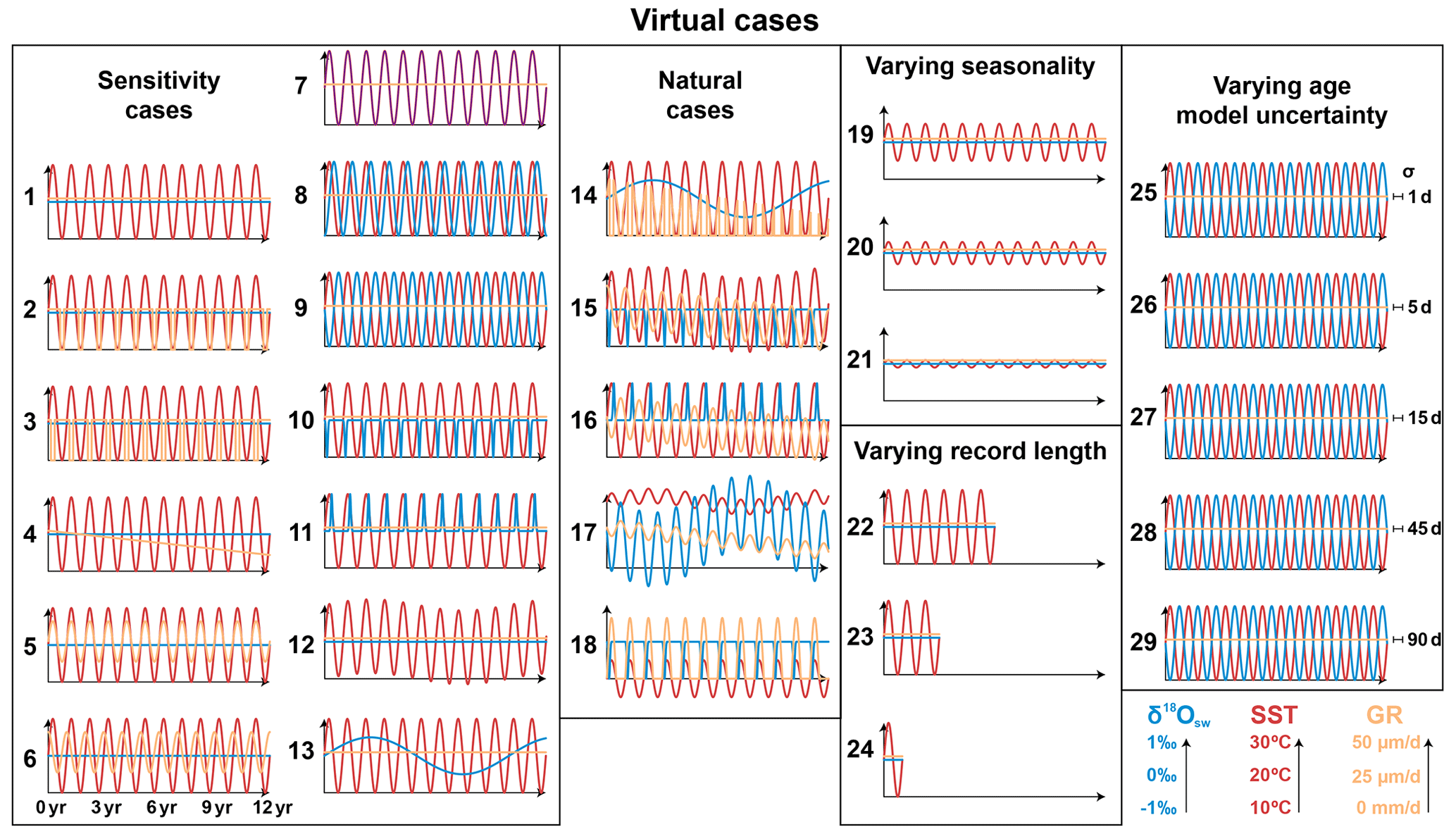
Figure 2Overview of time series of all virtual test cases. Colored curves represent time series of SST (red), δ18Ow (blue), and growth rate (orange, abbreviated as GR). Horizontal axes in all plots are 12 years long (see legend below case 6). Vertical axis of all plots has the same scale (SST: 10 to 30 ∘C; δ18Ow: −1 to +1 ‰; growth rate: 0–50 µm d−1; see legend in bottom right corner). Horizontal error bars and labels on the right side of cases 25–29 represent standard errors introduced to the age model (bars not to scale). The δ18Oc and Δ47 records resulting from these virtual datasets are provided in S6 (see also Fig. 3 for natural examples).
2.3.1 Cases 1–29: virtual environmental data, virtual proxy data
Virtual SST and δ18Ow time series were artificially constructed to test the effect of various SST and δ18Ow scenarios on the effectivity of the reconstruction methods. The default test case (case 1) contained an ideal 12-year sinusoidal SST curve with a period of 1 year (seasonality), a mean value of 20 ∘C, a seasonal amplitude of 10 ∘C, a constant δ18Ow value of 0 ‰, and a constant growth rate of 10 mm yr−1. Other cases contain various deviations from this ideal case (see also Fig. 2, Tables 1 and S1):
-
linear and/or seasonal changes in growth rate, including growth stops (cases 2–6, 14–18);
-
seasonal and/or multi-annual changes in δ18Ow (cases 7–11, 13–18);
-
multi-annual trends in SST superimposed on the seasonality (cases 12, 15, and 17);
-
variations in the seasonal SST amplitude (cases 19–21);
-
change in the total length of the time series (cases 22–24);
-
variation in uncertainty on the age of each virtual data point (cases 25–29).
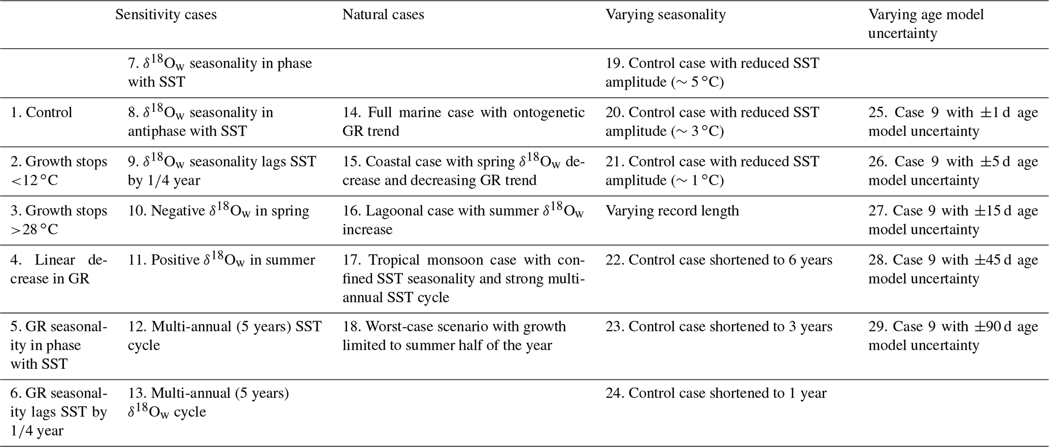
Table 1Overview of virtual cases 1–29 used to test the reconstruction methods. Case descriptions are abbreviated. Details on the SST, growth rate, and δ18Ow included in each case are described in Table S1. SST, growth rate, and δ18Ow records of all cases are shown in Fig. 2. GR: growth rate.
Comparison of the virtual time series (cases 1–29; Fig. 2) with the natural variability (cases 30–33; Fig. 3) shows that the virtual cases are not realistic approximations of natural variability in SST and δ18Ow. Natural SST and δ18Ow variability is not limited to the seasonal or multi-annual scale but contains a fair amount of higher-order (daily to weekly scale) variability. To simulate this natural variability, we extracted the seasonal component of SST and δ18Ow variability from our highest-resolution record of measured natural SST and SSS data (case 30: data from Texel, the Netherlands; see Sect. 2.3.2 and Fig. 3). The standard deviation of the residual variability of these data after subtraction of the seasonal cycle was used to add random high-frequency noise to the SST and δ18Ow variability in virtual cases. Note that while sub-annual environmental variability can be approximated by Gaussian noise (Wilkinson and Ivany, 2002), this representation is an oversimplification of reality. In the case of our Texel data, the SST and SSS residuals are not normally distributed (Kolmogorov–Smirnov test: D=0.010; and D=0.039; for SST and SSS residuals, respectively; see S2-4). SST and δ18Ow data from cases 1–29 were converted to the sampling domain and subsampled at a range of sampling resolutions following the same procedure applied to cases 30–33 (see Sect. 2.3.2).
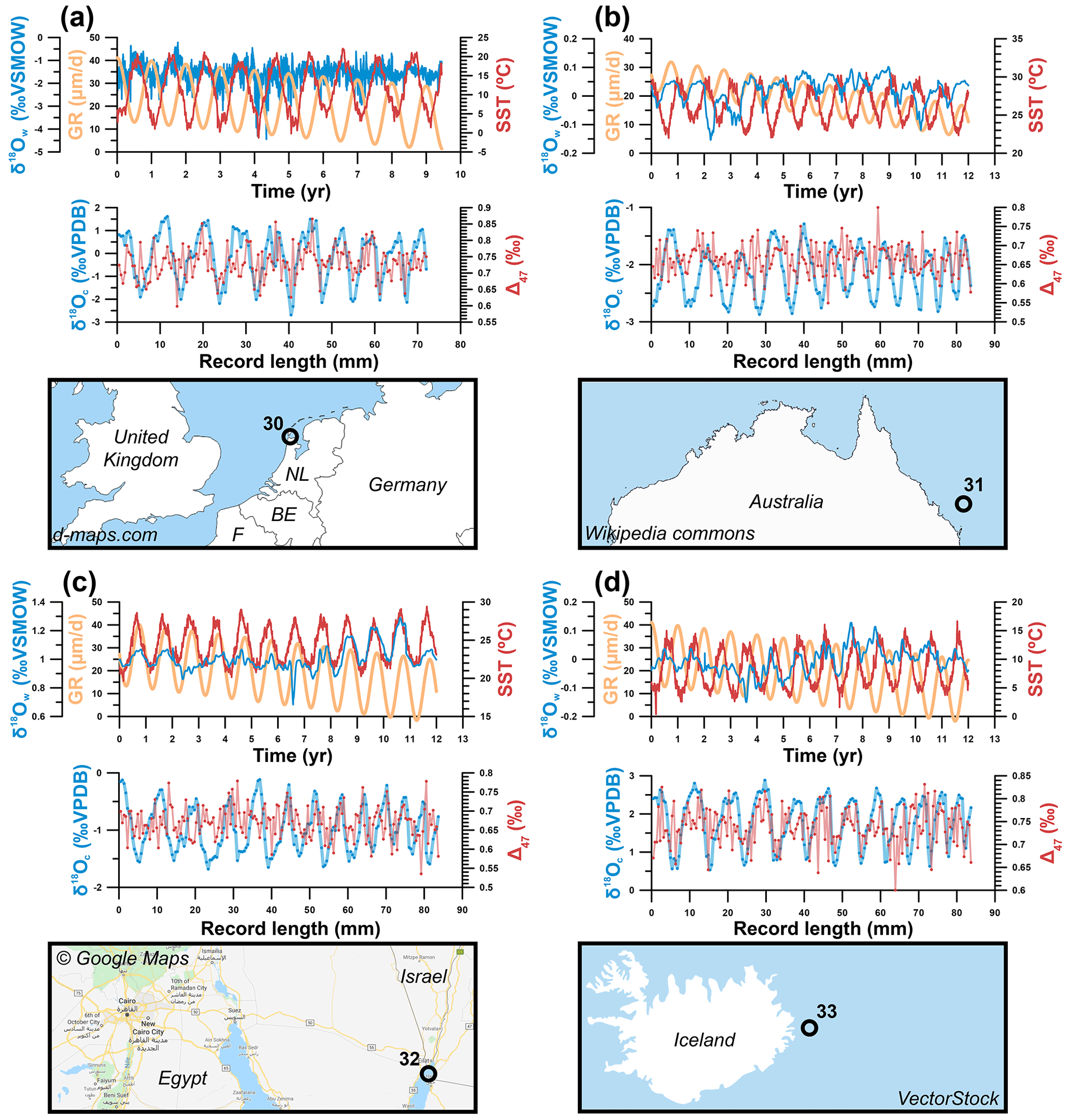
Figure 3Overview of the four cases of virtual data based on natural SST and SSS measurements explored in this study. (a) Case 30: tidal flats on the Wadden Sea, Texel, the Netherlands. (b) Case 31: Great Barrier Reef, Australia. (c) Case 32: Gulf of Aqaba between Egypt and Saudi Arabia. (d) Case 33: Atlantic Ocean east of Iceland. For all cases, graphs on top show environmental data, with SST plotted in red, δ18Ow in blue, and growth rate (abbreviated as GR) in orange (as in Fig. 2). The graph below shows virtual δ18Oc (blue) and Δ47 (red) records created from these data series using a sampling interval of 0.45 mm and including analytical noise (see Sect. 2.1 and 2.3.2). Note that the scale of vertical axes varies between plots.
2.3.2 Cases 30–33: measured environmental data, virtual proxy data
Four test cases were based on time series of real measured SST and SSS data from four different locations, which were selected to capture a variety of environments with different SST and SSS variability (see Fig. 3):
-
tidal flats of the Wadden Sea near Texel, the Netherlands (case 30);
-
Great Barrier Reef in Australia (case 31);
-
Gulf of Aqaba between Egypt and Saudi Arabia (case 32);
-
northern Atlantic Ocean east of Iceland (case 33).
Daily measurements of SST and SSS for cases 31–33 were obtained from worldwide open-access datasets of the National Oceanic and Atmospheric Administration (NOAA Physical Sciences Laboratory, 2021) and European Space Agency (Boutin et al., 2019), respectively. Hourly SST and SSS measured in situ in the Wadden Sea (case 30) were obtained from the Dutch Institute for Sea Research (NIOZ; Texel, the Netherlands). Since direct, in situ measurements of δ18Ow variability at a high temporal resolution were not available, δ18Ow was estimated from more widely available SSS data using a mass balance (Eqs. 1 and 2; following, e.g., Ullmann et al., 2010).
Here, we assume salinity (SSSsample) results from a mixture of a fraction (f) of isotopically light and low-salinity (δ18O ‰; SSSfreshwater=0) fresh water and a fraction (1−f) of ocean water (δ18O ‰; SSSocean=35), with negative amounts of freshwater contribution (f<0) representing net evaporation (SSSsample > SSSocean). The value for δ18Ow,freshwater was based on the δ18Ow of rain in the Netherlands (−8 ‰; Mook, 1970; Bowen, 2020). Applying this mass balance to the SSS record of the Wadden Sea tidal flats (case 30) results in δ18Ow values and an SSS–δ18Ow relationship in agreement with measurements in this region (Harwood et al., 2008). SST and δ18Ow time series for all cases are given in Supplement Data S4, and natural cases are plotted in Fig. 3.
For all virtual proxy datasets (cases 1–33), records of SST and δ18Ow were converted to the sampling domain (along the length of the record) by defining a virtual growth rate in the sampling direction. Adding this growth rate as a variable allowed us to test the sensitivity of approaches to changes in the extension rate of the archive, including hiatuses (growth rate 0). This is important because fluctuations in linear extension rate and periods in which no mineralization occurs (hiatuses or growth cessations) are common in all climate archives (e.g., Treble et al., 2003; Ivany, 2012). After conversion to the sampling domain, virtual aliquots were subsampled at equal distance from the SST and δ18Ow series of all cases using six sampling intervals: 0.1, 0.2, 0.45, 0.75, 1.55, and 3.25 mm. The four largest sampling intervals were chosen such that the standard growth rate (10 mm yr−1) was not an integer multiple of the sampling interval (e.g., 0.45 mm instead of 0.5 mm and 3.25 mm instead of 3 mm). This decision prevents sampling of the same parts of the seasonal cycle (e.g., same months) every year, which biases both the mean value and the precision of monthly SST and δ18Ow reconstructions. This bias towards certain parts of the seasonal cycle is much stronger at low sample sizes (large sampling intervals) and is illustrated in the Supplement Fig. S2.
2.3.3 Modern oyster: measured environmental data, measured proxy data
Environmental SST and δ18Ow data from the List Basin in Denmark (54∘59.25 N, 8∘23.51 E), where the modern oyster specimen lived, were obtained from local in situ measurements of SST and SSS described in Ullmann et al. (2010). Since direct, in situ measurements of δ18Ow variability at a high temporal resolution were not available, δ18Ow was estimated from more widely available SSS data using the mass balance described in Sect. 2.3.2. The value for δ18Ow,freshwater was based on the discharge-weighted average δ18Ow of water in the nearby Elbe and Weser rivers (see Ullmann et al., 2010). All δ18Ow values throughout the text are with reference to the VSMOW scale. Contrary to the virtual datasets (cases 1–33; see Sect. 2.3.1 and 2.3.2), the Ullmann et al. (2010) data were already available in the sampling domain; hence, no subsampling was required.
2.4 Conversion to δ18Oc and Δ47 data
After subsampling, SST and δ18Ow series (cases 1–33) were converted to δ18Oc and Δ47 using a carbonate model based on empirical relationships between Δ47–δ18Oc and SST–δ18Ow (Eqs. 3 and 4; Kim and O'Neil, 1997; Kele et al., 2015; Bernasconi et al., 2018) as well as the conversion of δ18O values from the VSMOW to the VPDB scale (Eq. 5; Brand et al., 2014).
For the modern oyster data (Ullmann et al., 2010; see Sect. 2.3.3), only the Δ47 data needed to be created because δ18Oc was directly measured. As a result, each case study yielded records of Δ47 and δ18Oc in the sampling domain and corresponding true SST and δ18Ow records in the time domain, allowing assessment of the reliability of the reconstruction approaches in different scenarios (Fig. 4). The result of applying these steps is illustrated with case 31 (Great Barrier Reef data, Fig. 5). All calculations for creating Δ47 and δ18Oc series in the sampling domain were carried out using the open-source computational software R (R core team, 2013), and scripts for these calculations are given in Supplement Data S7 and compiled in the documented R package “seasonalclumped” (de Winter, 2021a). All Δ47 and δ18Oc datasets are provided in Supplement Data S6.
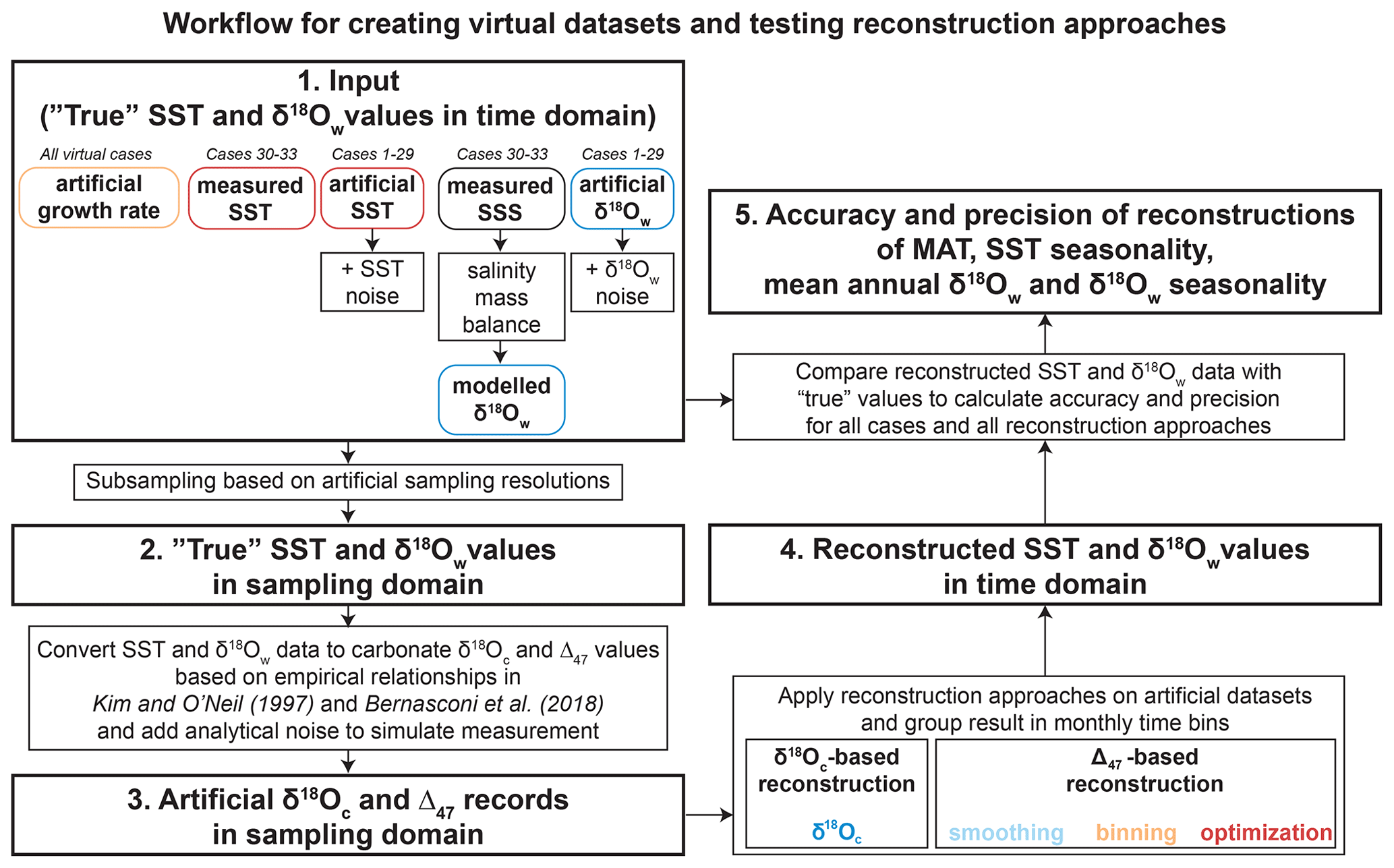
Figure 4Flow diagram showing the steps taken to create virtual data (Δ47 and δ18Oc; cases 1–33) and compare results of SST and δ18Ow reconstructions with the actual SST and δ18Ow data the record was based on (counterclockwise direction). Steps 1–3 outline the procedure for creating virtual Δ47 and δ18Oc datasets (see Sect. 2.3 and 2.4), step 4 shows the application of the different reconstruction methods to these virtual data (see Fig. 2 for details), and step 5 illustrates how the reconstructions are compared with the original (“true”) SST and δ18Ow data to calculate the accuracy and precision of the reconstruction approaches. Note that step 1 is different for cases 1–29 (based on fully artificial SST and δ18Ow records; Sect. 2.3.1) than for cases 30–33 (SST and δ18Ow records based on real SST and SSS data; see Sect. 2.3.2).

Figure 5An example of the steps highlighted in Fig. 4 using case 31 (Great Barrier Reef data) to illustrate the data processing steps. Virtual data plots include normally distributed measurement uncertainty in Δ47 and δ18Oc.
3.1 Real example
Measured (δ18Oc) and simulated (Δ47) data from the Pacific oyster from the Danish List Basin yielded estimates of SST and δ18Ow seasonality using all reconstruction approaches (Fig. 6). While a model of shell δ18Oc based on SST and SSS data closely approximates the measured δ18Oc record (Fig. 6c), basing SST reconstructions solely on δ18Oc data without any a priori knowledge of δ18Ow variability (assuming constant δ18Ow equal to the global marine value) leads to high inaccuracy in mean annual SST (Fig. 6d). Note that, in the absence of significant δ18Ow seasonality (as in this case study), seasonal temperature range reconstructions from δ18Oc measurements can be very accurate. However, assuming constant δ18Ow year-round may introduce considerable bias (see Figs. 7 and 8). The in-phase relationship between SST and SSS (Fig. 6b) slightly dampens the seasonal δ18Oc cycle, causing underestimation of temperature seasonality, while a negative mean annual δ18Ow value in the List Basin biases SST reconstructions towards higher temperatures. In terms of SST reconstructions, the smoothing, binning, and optimization approaches based on Δ47 and δ18Oc data yield more accurate reconstructions, albeit with reduced seasonality and a bias towards the summer season. The latter is a result of severely reduced growth rates in the winter season, which was therefore undersampled (see Fig. 6a and c). Approaches including Δ47 data also yield far more accurate δ18Ow estimates than the δ18O approach. However, the accuracy of δ18Ow seasonality and mean annual δ18Ow estimates is low in these approaches too, largely because of the limited sampling resolution, especially in winter. The optimization approach suffers from the strong in-phase relationship between SST and SSS, which obscures the difference between the δ18Ow effect and the temperature effect on shell carbonate. Yet, disentangling SST from δ18Ow seasonality is central to the success of the approach (see Sect. 4.2.3). Figure 6d does not show the precision of SST and δ18Ow estimates, which is much lower for the smoothing approach than for the binning and optimization approaches due to the limited data in the winter seasons (see Supplement Data S6). These results show that several properties of carbonate archives, such as growth rate variability, phase relationships between SST and δ18Ow seasonality, and sampling resolution, can impact the reliability of paleoseasonality reconstructions. The virtual and real data cases in this study were tailored to test the effects of these archive properties more thoroughly.

Figure 6(a) Plot of δ18Oc and (virtual) Δ47 data from a modern Pacific oyster (Crassostrea gigas; see Ullmann et al., 2010). (b) SST and δ18Ow data from the List Basin (Denmark) in which the oyster grew. (c) The fit between δ18Oc data and modeled δ18Oc calculated from SST and δ18Ow on which the shell age model was based. (d) A summary of the results of different approaches for reconstructing SST and δ18Ow from the δ18Oc and Δ47 data. The vertical colored bars show the reconstructed seasonal variability using all methods, with ticks indicating warmest month, coldest month, and annual mean. The grey horizontal bars show the actual seasonal variability in the environment. Precision standard deviations for monthly reconstructions are not shown but are given in Supplement Data S4.
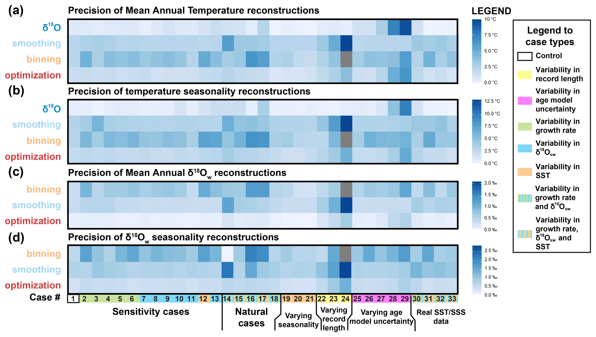
Figure 7Overview of the precision (propagated standard deviation of variability within reconstructions; see Sect. 2.2) of reconstructions of mean annual temperature (a), seasonal temperature range (b), mean annual δ18Ow (c), and seasonal range in δ18Ow (d), with higher values (darker colors) indicating lower precision (more variability between reconstructions) based on average sampling resolution (sampling interval of 0.45 mm). The different cases on the horizontal axis are color coded by their difference from the control case (case 1; see legend on the right-hand side). Grey boxes indicate cases for which reconstructions were not successful. All data on precision (standard deviation values) are provided in Supplement Data S4.
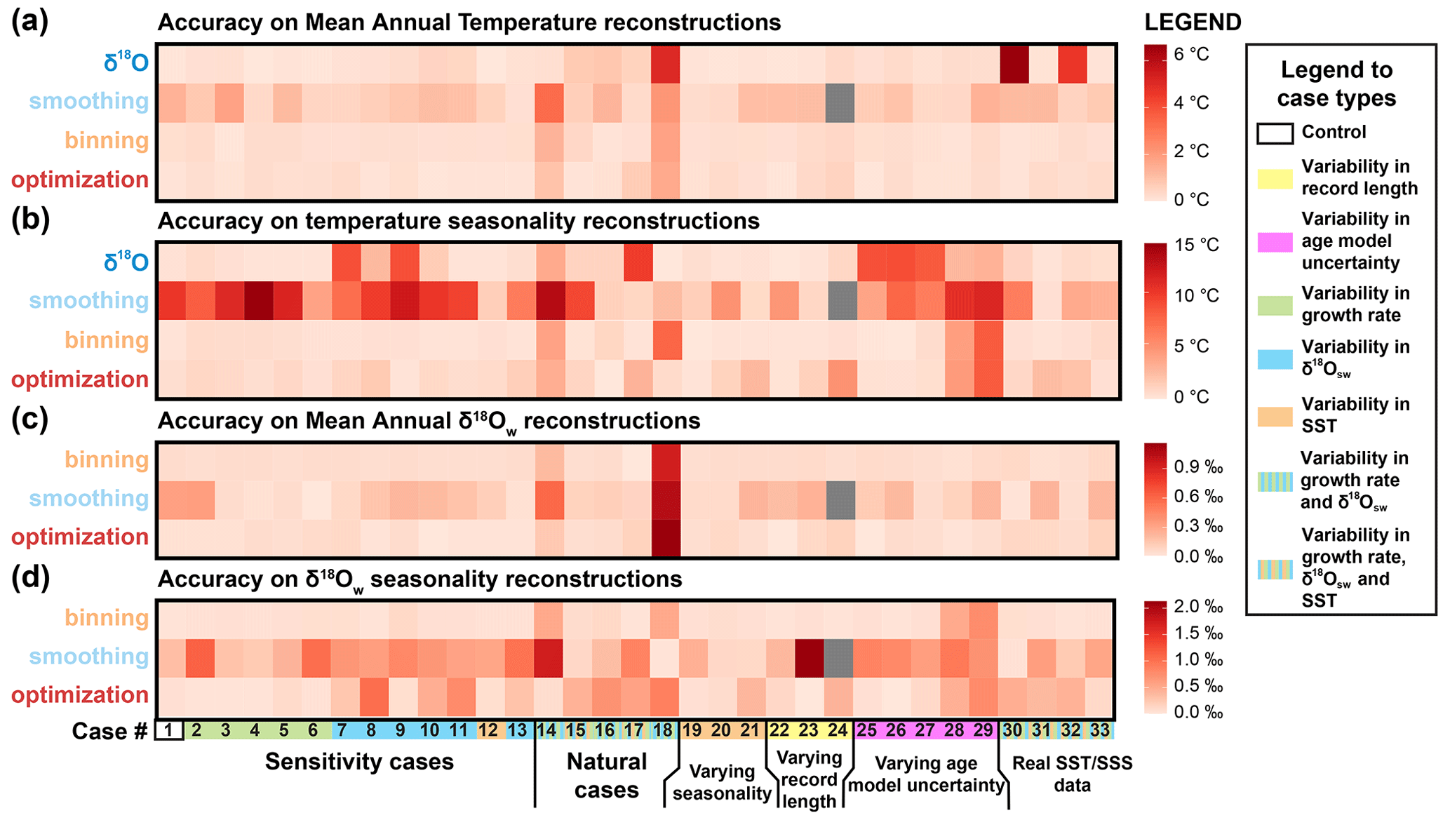
Figure 8Overview of the accuracy (absolute offset from “true” values) of reconstructions of mean annual temperature (a), seasonal temperature range (b), mean annual δ18Ow (c), and seasonal range in δ18Ow (d), with higher values (darker colors) indicating lower accuracy (higher offsets) based on average sampling resolution (sampling interval of 0.45 mm). The different cases on the horizontal axis are color coded by their difference from the control case (case 1; see legend on the right-hand side). Grey boxes indicate cases for which reconstructions were not successful. All data on accuracy (difference between reconstructed and true values) are provided in Supplement Data S4.
3.2 Case-specific results
A case-by-case breakdown of the precision (Fig. 7) and accuracy (Fig. 8) of reconstructions using the four approaches shows that the reliability of reconstructions varies significantly between approaches and is highly case-specific. In general, precision is highest in δ18O reconstructions, followed by optimization and binning, with smoothing generally yielding the worst precision. Average standard deviations of the underperforming methods (binning and smoothing) are up to 2–3 times larger than those of δ18O (e.g., 3.9 and 3.5 ∘C vs. 1.3 ∘C for δ18O MAT reconstructions; see also the Supplement). It is worth noting that precision of δ18O-based estimates is mainly driven by measurement precision (which is better for δ18Oc than for Δ47 measurements; see Sect. 4.1.1). Δ47-based reconstructions lose precision due to the higher error in Δ47 measurements and the method used for combining measurements for seasonality reconstructions. On a case-by-case basis, the hierarchy of approaches can vary, especially if strong variability in growth rate is introduced, such as in case 14, in which the size of hiatuses in the record increases progressively, and in case 18, in which half of the year is missing due to growth hiatuses (see Table 1, Supplement Data S1 and S4). Of the Δ47-based methods (smoothing, binning, and optimization), optimization is rarely outcompeted in terms of precision in both SST and δ18Ow reconstructions.
The comparison based on precision alone is misleading, as the most precise approach (δ18O) runs the risk of being highly inaccurate (offsets exceeding 4 ∘C in some MAT reconstructions; see Fig. 8a), especially in cases based on natural SST and SSS measurements (cases 30–33). The smoothing approach also often yields highly inaccurate results, especially in cases with substantial variability in δ18Ow (e.g., cases 9–11; Fig. 8). Optimization and binning outcompete the other methods in most circumstances in terms of accuracy. Binning outperforms optimization in reconstructions of δ18Ow seasonality, making it the overall most accurate approach. Interestingly, optimization is less accurate, specifically in cases with sharp changes in growth rate in summer (e.g., cases 11, 14, 16, and 17), while binning performs better in these cases. Reconstructions of mean annual SST and δ18Ow in case 18 are especially inaccurate regardless of which method is applied. This extreme case with growth only during half of the year combined with seasonal fluctuations in both SST and δ18Ow presents a worst-case scenario for seasonality reconstructions, leading to strong biases in mean annual temperature reconstructions. In situations like case 18, the optimization approach is most accurate in MAT and SST seasonality reconstructions, but δ18Ow is more accurately reconstructed using the binning approach. Finally, it is worth noting that in natural situations (Fig. 3), variability in SST almost invariably has a larger influence on δ18Oc and Δ47 records than δ18Ow such that fluctuations in δ18Oc records closely follow the SST seasonality, even in cases with relatively large δ18Ow variability (e.g., case 30). Chronologies based on these δ18Oc fluctuations are therefore generally accurate.
3.3 Effect of sampling resolution
As expected, increasing the temporal sampling resolution (i.e., number of samples per year) almost invariably increases the precision and accuracy (Fig. 9) of reconstructions using all methods. An exception to this rule is the precision of δ18O reconstructions, which decreases with increasing sampling resolution (see Fig. 9c–d). Precision standard deviations of all Δ47-based approaches eventually converge with the initially much higher precision of δ18O reconstructions when sampling resolution increases. However, the sampling resolution required for Δ47-based reconstructions to rival or outcompete the δ18O reconstructions differs, with optimization requiring lower sampling resolutions than the other methods (e.g., 20–40 samples per year compared to 40–80 samples per year for smoothing and binning; Fig. 9a–d). Accuracy also improves with sampling resolution (Fig. 9e–h). When grouping all cases together, it becomes clear that δ18O reconstructions can only approach the accuracy of Δ47-based approaches for reconstructions of MAT. Seasonality in both SST and δ18Ow is most accurately reconstructed using binning, and the smoothing approach once again performs worst.
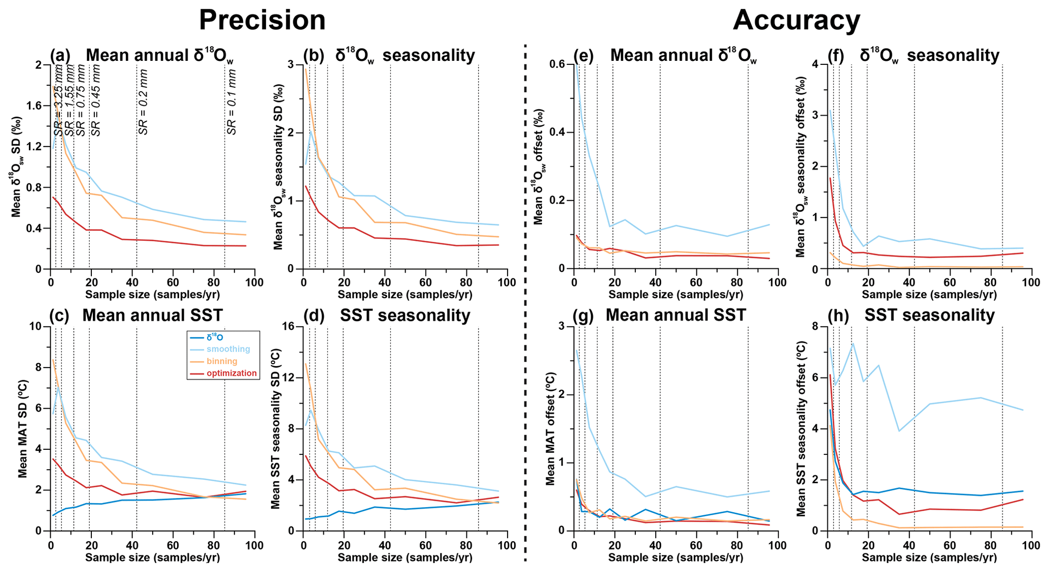
Figure 9Effect of sampling resolution (in samples per year; see S5) on the precision (1 standard deviation) of results of reconstructions of mean annual δ18Ow (a), seasonal range in δ18Ow (b), mean annual SST (c), and seasonal range in SST (d). Effect on the accuracy (absolute offset from actual value) of results of reconstructions of mean annual δ18Ow (e) and seasonal range in δ18Ow (f), mean annual SST (g), and seasonal range in SST (h). Color coding follows the scheme in Figs. 1 and 4.
3.4 Resolving SST seasonality
Comparison of cases 19, 20, and 21 (SST seasonality of 9.7, 5.7, and 2.1 ∘C, respectively) with control case 1 (SST seasonality of 19.3 ∘C) shows how changes in the seasonal SST range affect the precision of measurements (Fig. 10; see also Table 1 and Supplement Data S1). The data reconfirm that δ18O reconstructions are the most precise, which is a deceptive statistic given the risk of highly inaccurate results with this approach (see Fig. 8). Taking into consideration only analytical uncertainty, all approaches except for smoothing can confidently resolve at least the highest SST seasonality within a significance level of 2 standard deviations (∼95 %) using a moderate sampling resolution (mean of all resolutions shown in Fig. 10). Increasing sampling resolution improves the precision of Δ47-based reconstructions (see Fig. 9d), so high sampling resolutions (0.1 or 0.2 mm) allow smaller seasonal differences to be resolved. When random sub-annual variability is added to the SST and δ18Ow records (see Sect. 2.3.1), the minimum seasonal SST extent that can be resolved decreases for all approaches (Fig. 10b and c). Nevertheless, δ18O and optimization reconstructions remain able to resolve a relatively small SST seasonality of 2–4 ∘C.
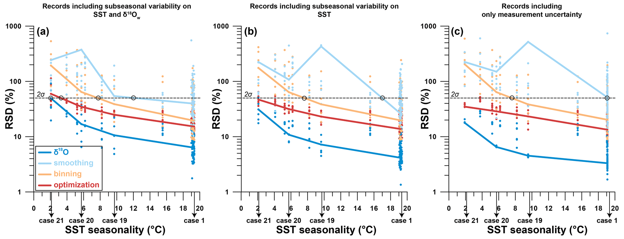
Figure 10Effect of SST seasonality range (difference between warmest and coldest month) in the record on the relative precision of SST seasonality reconstructions (RSD, defined as 1 standard deviation divided by the mean value). (a) Precision results if random variability (“weather patterns”) in both SST and δ18Ow as well as measurement uncertainty is added to the records (see Sects. 2.3.1 and S1). (b) Precision of records with random variability in SST and measurement uncertainty only. (c) Precision if only measurement uncertainty is considered. Color coding follows the scheme in Figs. 1 and 4. Shaded dots represent results at various sampling resolutions, while bold lines are averages for all reconstruction approaches. Black circles highlight the places where curves cross the threshold of 2 standard deviations, which indicates the minimum SST seasonality that can be resolved within 2 standard deviations (∼95 % confidence level) using the reconstruction approach.
3.5 Effect of record length
The effect of variation in the length of the record was investigated by comparing cases 22, 23, and 24 (record lengths of 6 years, 3 years, and 1 year, respectively) with the control case (record length of 12 years; see Fig. 11 and Table 1). The precision of MAT and SST seasonality reconstructions slightly increases in larger datasets (longer records) for optimization and binning, but not for smoothing and δ18O reconstructions. Differences between reconstruction approaches remain relatively constant regardless of the length of the record, with the precision hierarchy generally remaining intact (δ18O > optimization > binning > smoothing). However, in very short records (1–2 years) smoothing generally gains an advantage over other Δ47-based methods due to its lack of sensitivity to changes in the record length, and binning reconstructions are not precise enough to resolve SST seasonality within 2 standard deviations (∼95 % confidence level). Variation in precision is largely driven by the very low precision of reconstructions in records with low sampling resolutions (sampling intervals of 1.55 mm or 3.25 mm; see also Fig. 9a–d). As a result, most of the reduction in precision in shorter records can be mitigated by denser sampling.
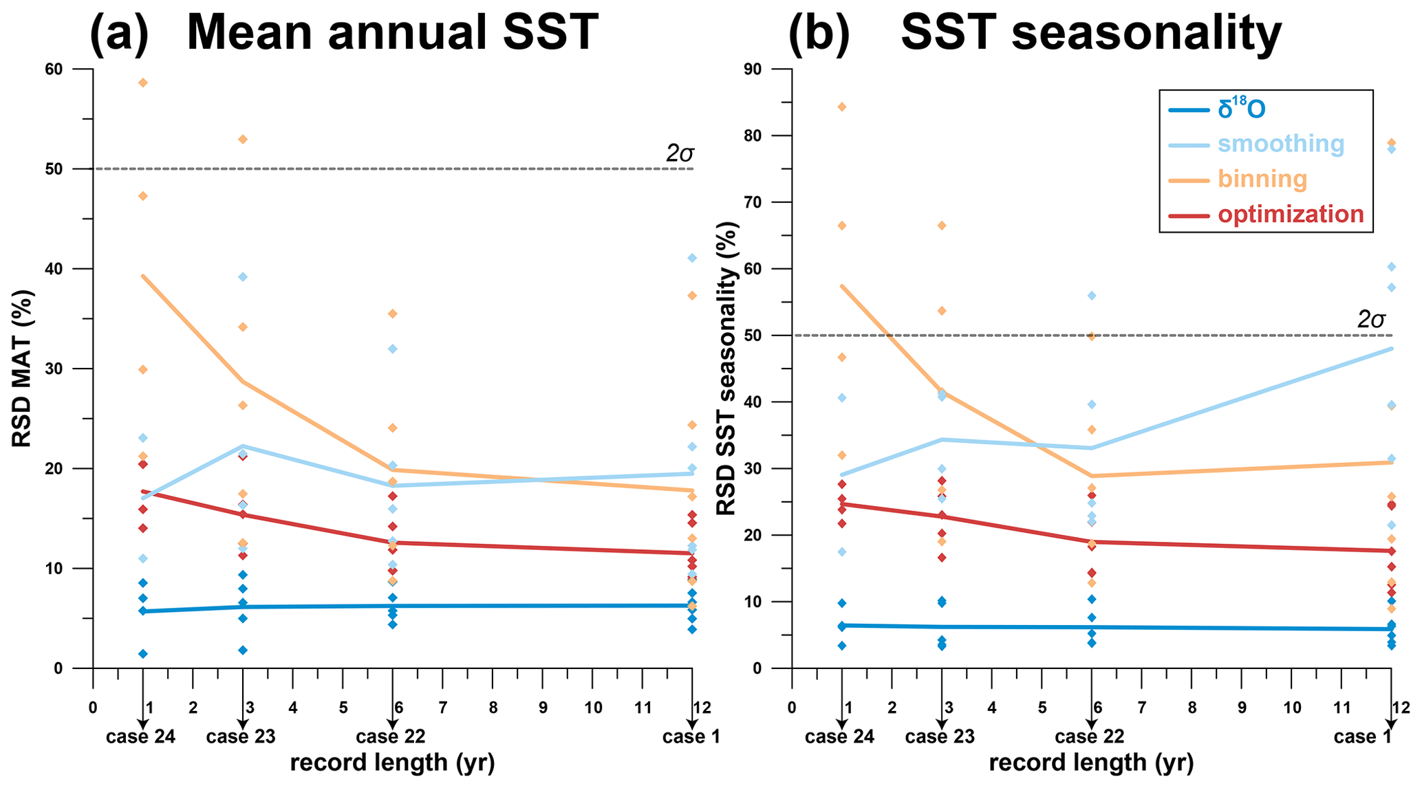
Figure 11Effect of record length (in years) on the relative precision (1 standard deviation as a fraction of the mean value) of results of reconstructions of mean annual SST (a) and SST seasonality (b). Colored dots represent results for the six different sampling resolutions. Solid lines connect averages for cases 1, 22, 23, and 24 for each reconstruction approach.
3.6 Effect of age model uncertainty
Uncertainty in the age model has a significant effect on both the precision and the accuracy (Fig. 12) of reconstructions using all approaches. The δ18O reconstructions are most strongly affected by uncertainties in the age model and suffer from a large decrease in precision with increasing age model uncertainty (Fig. 12c–d). The high precision of the δ18O approach in comparison with the Δ47 approaches quickly disappears when age model uncertainty increases beyond 20–30 d. The accuracy of δ18Oc-based SST seasonality reconstructions initially improves with age model uncertainty (Fig. 12h). However, this observation is likely caused by the fact that age model uncertainty was compared based on conditions in case 9, which features a phase offset between SST and δ18Ow seasonality, causing the δ18O method to be highly inaccurate even without age model uncertainty. The precision of smoothing and optimization approaches also decreases with increasing age model uncertainty (Fig. 12a–d), and the optimization approach loses its precision advantage over the binning and smoothing approaches when age model uncertainty increases beyond 30 d. The monthly binning approach is most resilient against increasing age model uncertainty. Seasonality reconstructions through both the binning and optimization approach quickly lose accuracy when age model uncertainty increases, but the accuracy of the smoothing approach remains the worst of all Δ47-based approaches regardless of age model uncertainty, except in the case of δ18Ow seasonality at exceptionally high (>60 d) age uncertainty (Fig. 12e–h).
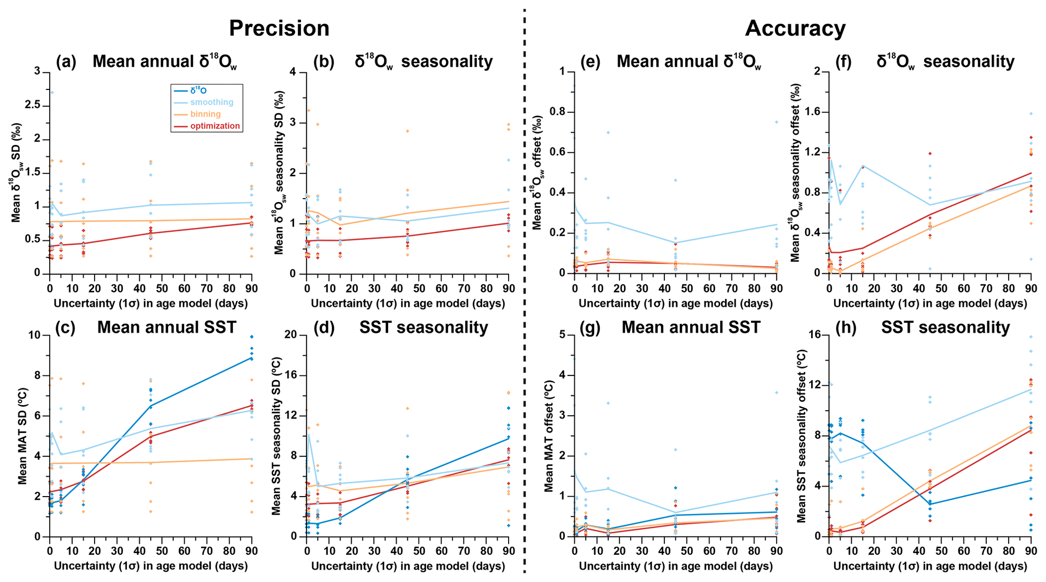
Figure 12Effect of uncertainty in the age model on the precision (standard deviation on estimate) of results of reconstructions of mean annual δ18Ow (a), seasonal range in δ18Ow (b), mean annual SST (c), and seasonal range in SST (d). Effect of uncertainty in the age model on the accuracy (offset from true value) of results of reconstructions of mean annual δ18Ow (e), seasonal range in δ18Ow (f), mean annual SST (g), and seasonal range in SST (h). Color coding follows the scheme in Figs. 1 and 4.
4.1 Performance of reconstruction approaches
4.1.1 δ18Oc vs Δ47-based reconstructions
Figure 13 summarizes the general reliability of the four approaches. δ18O reconstructions are generally less accurate than Δ47-based reconstructions (especially binning and optimization; see also Supplement Data S9). This is a consequence of the assumption that δ18Ow remains constant year-round and that one knows its true value. Both these assumptions are problematic in the absence of independent evidence of the value of δ18Ow, especially in deep time settings (see, e.g., Veizer and Prokoph, 2015; Henkes et al., 2018). The risk of this assumption is made clear when comparing cases in which δ18Ow is indeed constant year-round at the assumed value (0 ‰; e.g., cases 1–6 and 19–24) with cases in which shifts in δ18Ow occur, especially when these shifts are out of phase with respect to the SST seasonality (e.g., cases 9–11, 18, and 25–33; Fig. 8c–d). Cases mimicking or based on natural SST and SSS variability (cases 14–18 and 30–33) as well as the modern oyster data (Fig. 6) yield stronger inaccuracies in MAT and seasonality reconstructions, showing that even in many modern natural circumstances the assumption of constant δ18Ow is problematic.
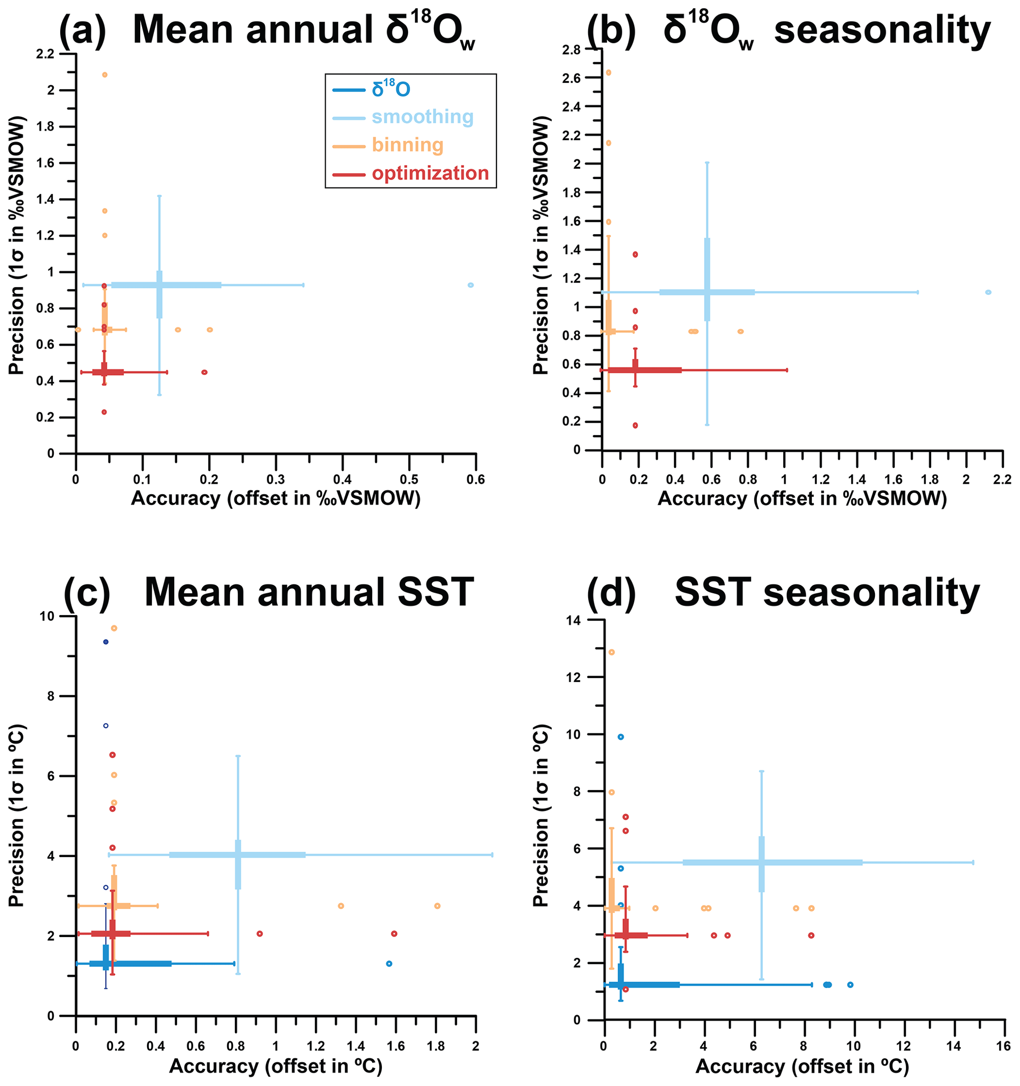
Figure 13Overview of averages and ranges of accuracy (absolute offset from real value) and precision (1 standard deviation from the mean) for mean annual δ18Ow (a), seasonal range in δ18Ow (b), mean annual SST (c), and seasonal range in SST (d) within all cases using the four different reconstruction approaches. Color coding follows the scheme in Figs. 1 and 4. Box–whisker plots for precision and accuracy cross at their median values, and outliers (colored symbols) are identified based on 2× the interquartile difference (thick lines).
It is important to consider that the value of mean annual δ18Ow remained very close to the assumed value of 0 ‰ (within 0.15 ‰) in all cases except for natural data cases 30 (−1.55 ‰), 32 (1.01 ‰; see Supplement Data S5), and the real oyster data (−1.42 ‰; Fig. 5). The SST values of these cases reconstructed using δ18Oc data show large offsets from their actual values (+6.7 ∘C, −4.7 ∘C, and +10.3 ∘C for case 30, case 32, and the real oyster data, respectively; see Figs. 6 and 8 and Supplement Data S5). These offsets are equivalent to the temperature offset one might expect from inaccurately estimating δ18Ow ( ∘C/‰; Kim and O'Neil, 1997) and are only rivaled by the offset in MAT reconstructions of case 18 (+5.0 ∘C), which has growth hiatuses obscuring the coldest half of the seasonal cycle. The fact that such differences in δ18Ow exist even in modern environments should not come as a surprise, given the available data on worldwide variability of δ18Ow (at least −3 ‰ to +2 ‰; e.g., LeGrande and Schmidt, 2006) and SSS (30 to 40; ESA, 2020) in modern ocean basins. However, it should warrant caution in using δ18Oc data for SST reconstructions even in modern settings. Implications for deep time reconstructions are even greater, given the uncertainty and variability in global average (let alone local) δ18Ow values (Jaffrés et al., 2007; Veizer and Prokoph, 2015). The complications of using δ18Oc as a proxy for marine temperatures in deep time are discussed in detail in O'Brien et al. (2017) and Tagliavento et al. (2019). Complications arising from variability in δ18Ow are more serious in climate records from euryhaline carbonate producers (e.g., oysters) than from stenohaline organisms (e.g., corals), as they are mainly driven by salinity fluctuations. For example, seasonal salinity variability in the North Sea at offshore sites away from freshwater sources can be as low as 0.25 (Harwood et al., 2008) compared to 3–4 in the coastal Texel site simulated in case 30. Given this variability, studies using the δ18Oc proxy for SST reconstructions are recommended to either reconstruct δ18Ow through additional measurements (e.g., including clumped isotope analysis) or constrain δ18Ow variability through isotope-enabled modeling (e.g., Williams et al., 2009)
The analytical uncertainty of individual δ18Oc aliquots (typically 1 SD of 0.05 ‰; e.g., de Winter et al., 2018) represents only ∼1.1 % of the variability in δ18Oc over the seasonal cycle (∼4.3 ‰ for the default 20 ∘C seasonality in case 1, following Kim and O'Neil, 1997). This is much smaller than the analytical uncertainty of Δ47 (typically 1 SD of 0.02–0.04 ‰; e.g., Fernandez et al., 2017; de Winter et al., 2021), which equates to 25 %–50 % of the seasonal variability in Δ47 (∼0.08 ‰ for 20 ∘C seasonality, following Bernasconi et al., 2018; see Supplement Data S7). This roughly 20-fold difference in relative precision causes δ18Oc-based SST reconstructions to be much more precise (see Figs. 7, 9–12) than those based on Δ47 and forces the necessity of grouping Δ47 data in reconstructions. However, as discussed above, the high precision of δ18O reconstructions is a misleading statistic if they are highly inaccurate.
Our results show that paleoseasonality reconstructions based on δ18Oc can only be relied upon if there is strong independent evidence of the value of δ18Ow and if significant sub-annual variability in δ18Ow (>0.3 ‰, equivalent to 2–3 ∘C SST variability; see Figs. 9–10; Kim and O'Neil, 1997) can be excluded with confidence. Examples of such cases include fully marine environments unaffected by influxes of (isotopically light) fresh water or evaporation (increasing δ18Ow; Rohling, 2013). Carbonate records from environments with more stable δ18Ow conditions include, for example, the A. islandica bivalves from considerable depth (30–50 m) in the open-marine northern Atlantic (e.g., Schöne et al., 2005, on which case 33 is based). However, even here variability in δ18Osw due to, for example, the shifting influence of different bottom-water masses cannot be fully excluded. Previous reconstruction studies show that δ18Ow in smaller basins is heavily influenced by the processes affecting δ18Ow on smaller scales, such as local evaporation and freshwater influx from nearby rivers (e.g., Surge et al., 2001; Petersen et al., 2016). Consequently, accurate quantitative reconstructions of seasonal range in shallow marine environments with extreme seasonality may not be feasible using the δ18O approach because these environments are invariably characterized by significant fluctuations in δ18Ow and growth rate.
While variability in δ18Ow compromises accurate δ18O-based seasonality reconstructions, the compilation in Fig. 3 shows that its influence on the δ18O records is too small to affect the shape of the record to such a degree that seasonality is fully obscured. While natural situations with δ18Ow fluctuations large enough to totally counterbalance the effect of temperature seasonality on δ18O records are imaginable, these cases are likely rare. This means that chronologies based on δ18O seasonality, which are a useful tool to anchor seasonal variability in the absence of independent growth markers (e.g., Judd et al., 2018; de Winter, 2021b), are reliable in most natural cases.
4.1.2 Seasonality reconstructions using moving averages (smoothing)
Of the three methods for combining Δ47 data, the smoothing approach clearly performs worst for all four reconstructed parameters (MAT, SST seasonality, mean annual δ18Ow and δ18Ow seasonality) in terms of both accuracy and precision (Fig. 13). While applying a moving average may be a good strategy for lowering the uncertainty of Δ47-based temperature reconstructions in a long time series (e.g., Rodríguez-Sanz et al., 2017), the method underperforms in cases in which the baseline and amplitude of a periodic component (e.g., MAT and SST seasonality) are extracted from a record. This is likely due to the smoothing effect of the moving average, which reduces the seasonal cycle and causes highly inaccurate seasonality reconstructions (offsets amounting to >6 ∘C; Fig. 13). This bias is especially detrimental in cases in which the seasonal cycle is obscured by seasonal growth halts (e.g., case 18), multi-annual trends in growth (e.g., cases 4, 14, and 17), and multi-annual trends in SST (e.g., cases 15 and 17; see Figs. 7 and 8). The poor performance of the smoothing approach can be slightly mitigated by increasing sampling resolution (Fig. 9), but even at high sampling resolutions (every 0.1 or 0.2 mm) the method still fails to reliably resolve seasonal SST ranges below 5 ∘C, even in idealized cases (cases 19–21; Fig. 10). Increasing the number of samples by analyzing longer records does not improve the result because smoothing of the seasonal cycle by a moving average window introduces the same dampening bias if the temporal sampling resolution (number of samples per year) remains equal (Fig. 11).
More critically, employing the smoothing method may give the illusion that seasonality is more reduced and severely bias reconstructions. This bias highlights the importance of using the official meteorological definition of seasonality as the difference between the averages of the warmest and coldest month in paleoseasonality work (O'Donnell and Ignizio, 2012). This definition is much more robust than the “annual range” often cited based on maxima and minima in δ18Oc records. This annual range strongly depends on sampling resolution, which is typically <12 samples per year (Goodwin et al., 2003), equivalent to the third lowest sampling interval (0.75 mm) simulated in this study. Therefore, we strongly recommend that future studies adhere to the monthly definition of seasonality to foster comparison between studies. While interannual variability is lost by combining data from multiple years into monthly averages, this approach increases the precision, accuracy, and comparability of paleoseasonality results. Interannual variability can still be discussed from raw data plotted in the time or sampling domain.
4.1.3 Monthly binning, sample size optimization, and age model uncertainty
Overall, the most reliable paleoseasonality reconstructions can be obtained from either binning or optimization (Fig. 13). In general, optimization is slightly more precise, while binning yields more accurate estimates of the seasonal range in SST and δ18Ow (Fig. 13b and d). The more flexible combination of aliquots in the optimization routine yields improved precision (especially for mean annual averages) in cases in which parts of the record are undersampled or affected by hiatuses and simultaneous fluctuations in both SST and δ18Ow (e.g., cases 3–6, 14–18, 30–33). The downside of this flexibility is that in the case of larger sample sizes, the seasonal variability may be dampened, like in the smoothing approach (see Sect. 4.1.2). This apparent dampening effect may be reduced by allowing the sample size of summer and winter samples to vary independently in the optimization routine at the cost of higher computational intensity due to the larger number of sample size combinations (see Sects. 2.1 and 4.2.2). The rigid grouping of data into monthly bins in binning prevents this dampening and therefore yields slightly more accurate estimates of seasonal ranges in SST and δ18Ow. A caveat of binning is that it requires a very reliable age model of the record, at least on a monthly scale. If the age model has a large uncertainty, there is a risk that samples are grouped in the wrong month, which compromises the accuracy of binning reconstructions, especially for reconstructions of seasonal range (Fig. 12h). This problem is exacerbated by potential phase shifts between seasonality in paleoclimate variables (SST and δ18Ow) and calendar dates, which may occur in the presence of a reliable age model.
Previous authors attempted to circumvent the dating problem by analyzing high-resolution δ18Oc transects and subsequently sampling the seasonal extremes for clumped isotope analyses (Keating-Bitonti et al., 2011; Briard et al., 2020). While this approach does not require sub-annual age models, it has several disadvantages compared with binning and optimization approaches: firstly, it requires separate sampling for δ18Oc and Δ47, which may not be possible in high-resolution carbonate archives due to sample size limitations. Analyzing small aliquots for combined δ18Oc and Δ47 analyses consumes less material. Secondly, individual summer and winter temperature reconstructions require large (>1.5 mg; e.g., Fernandez et al., 2017) Δ47 samples from seasonal extremes, which causes more time averaging than the approaches combining small aliquots. Finally, the position of seasonal extremes estimated from the δ18Oc record may not reflect the true seasonal extent if seasonal SST and δ18Ow cycles are not in phase (as in case 9), causing seasonal Δ47-based SST reconstructions to underestimate the temperature seasonality. In such cases, δ18Oc and Δ47 analyses of small aliquots allow the seasonality in SST and δ18Ow to be disentangled, yielding more accurate seasonality reconstructions.
Techniques for establishing independent age models for climate archives range from counting of growth layers or increments (Schöne, 2008; Huyghe et al., 2019), to modeling and extracting of rhythmic variability in climate proxies through statistical approaches (e.g., De Ridder et al., 2007; Goodwin et al., 2009; Judd et al., 2018; de Winter, 2021b), and interpolation of uncertainty on absolute dates (e.g., Scholz and Hoffman, 2011; Meyers, 2019; Sinnesael et al., 2019). While propagating uncertainty in the data on which age models are based onto the age model is relatively straightforward, errors in underlying a priori assumptions, such as linear growth rate between dated intervals, (quasi-)sinusoidal forcing of climate cycles, and the uncertainty in human-generated data like layer counting, are very difficult to quantify (e.g., Comboul et al., 2014) and may not be normally distributed. Results of cases 25–29 show that uncertainties in the age domain can significantly compromise reconstructions (Fig. 12). Within the scope of this study, only the effect of symmetrical, normally distributed uncertainties in an artificial case with phase-decoupled SST and δ18Ow seasonality (case 9) was tested. The effects of other types of uncertainties on the reconstructions remain unknown, highlighting an unknown uncertainty in paleoseasonality and other high-resolution paleoclimate studies that may introduce bias or lead to overly optimistic uncertainties in reconstructions. Future research could quantify this unknown uncertainty by propagating estimates of various types of uncertainty on depth values of samples and on the conversion from sampling to time domain in age models.
4.2 Conditions influencing success of reconstructions
The reliability (accuracy and precision) of SST and δ18Ow reconstructions depends on case-specific conditions. The range of cases tested in this study allowed us to evaluate the effect of variability in SST, growth rate, δ18Ow, sampling resolution, and record length relative to the control case (case 1; see Supplement Data S1). A summary of the effects of these changes is given in Table 2.
Table 2Qualitative summary of the effects of changes in variables relative to the ideal case on reconstructions using the four approaches. The “cases” column lists cases in which the changes in the respective variable relative to the control case (case 1) were represented (see Tables 1 and S1). 0: negligible effect, +: weak increase in uncertainty, : moderate increase in uncertainty, : strong increase in uncertainty. Precision and accuracy of all tests are given in S9.

4.2.1 SST variability
Variability in water temperature most directly affects the proxies under study. By default (case 1), SST varies sinusoidally around a MAT of 20 ∘C with an amplitude of 10 ∘C (see Sect. 2.3.1, Fig. 2, and Supplement Data S1). In cases in which multi-annual variability in SST is simulated (e.g., cases 15 and 17), the accuracy of SST reconstructions using δ18O and optimization is reduced, while the binning approach is less strongly affected. Examples of such multi-annual cyclicity include the El Niño–Southern Oscillation (ENSO; Philander, 1983) and North Atlantic Oscillation (NOA; Hurrell, 1995). The effect is especially large in case 17, which simulates a tropical environment with reduced SST seasonality and a strong multi-annual cyclicity. This type of environment is analogous to the environment of tropical shallow-water corals, which are often used as archives for ENSO variability (e.g., Charles et al., 1997; Fairbanks et al., 1997), and is similar to tropical cases from the Australian Great Barrier Reef (case 31) and the Red Sea (case 32; see Fig. 3). We therefore recommend using the binning approach on carbonate records in which multi-annual cyclicity is prevalent and if a reliable age model can be established for these records (as in, e.g., Sato, 1999; Scourse et al., 2006; Miyaji et al., 2010).
4.2.2 Growth rate variability and hiatuses
Figures 7 and 8 show that variations in the growth rate of records, including the occurrence of hiatuses, have a strong effect on reconstructions, especially using the smoothing approach. In general, hiatuses and slower growth reduce the precision of monthly SST and δ18Ow reconstructions by reducing mean temporal sampling resolution (samples per year; see Fig. 9) and because parts of the record are undersampled. The effect on accuracy depends strongly on the timing of changes in growth rate or the occurrence of hiatuses. Cases 2–6 simulate specific growth rate effects and can be used to test these differences. The smoothing method is especially sensitive to changes in growth rate that take place in specific seasons, such as hiatuses in winter (case 2) or summer (case 3) and growth peaks in summer (case 5) or spring (case 6). The other reconstruction approaches are less affected by this bias because they generally do not mix samples from different seasons. The δ18O method is especially well suited to deal with changes in growth rate because it does not require combining different aliquots for accurate SST reconstructions. The binning and optimization approaches are slightly less reliable in cases in which the growth rate decreases linearly or seasonally along the entire record (cases 4–6; Fig. 2). Because these two methods consider all samples in the records at once, they are more sensitive to changes in temporal sampling resolution along the record. It is worth noting that optimization is especially sensitive to sharp changes in growth rate in summer (e.g., cases 11, 14, 16, and 17) because those conditions force the optimization routine to use larger sample sizes or include samples outside the warmest month for summer temperature estimates. A potential solution to this problem could be to allow sample sizes of summer and winter groups to vary independently in the optimization routine (see Sect. 2.1). This would allow sample size in the undersampled season (in this case, summer) to become larger than that at the other end of the δ18Oc spectrum, reducing uncertainty in the more densely sampled season and therefore improving the entire seasonality reconstruction.
A worst-case scenario is represented by case 18, in which the cold half of the year is not recorded. Such cases result in strong biases in reconstructions of mean annual and seasonal ranges in SST and δ18Ow, regardless of which method is used. In such extreme cases the record simply contains insufficient information to reconstruct variability in growth rate, SST, and δ18Ow, and it seems that no statistical method would enable this missing information to be recovered. The solution for these reconstructions would be to establish reliable age models, independent of δ18O or Δ47 data, which show that a large part of the seasonal cycle is missing. All methods used in this study rely on a conversion of SST and δ18Ow reconstructions to the time domain to define monthly time bins. This conversion breaks down in fossil examples when the seasonal cycle cannot be extracted from the archive, which happens when half of the seasonal cycle or more is obscured by growth hiatuses, as exemplified in case 18.
While hiatuses encompassing half of the seasonal cycle are uncommon, changes in growth rate are common in accretionary carbonate archives because conditions for (biotic or abiotic) carbonate mineralization often vary over time. This variability is either driven by biological constraints, such as senescence (e.g., Schöne, 2008; Hendriks et al., 2012), the reproductive cycle (Gaspar et al., 1999), and stress (Surge et al., 2001; Compton et al., 2007), or by variations in the environment that promote or inhibit carbonate production, such as seasonal variations in temperature (Crossland, 1984; Bahr et al., 2017) or precipitation (Dayem et al., 2010; Van Rampelbergh et al., 2014). In general, such conditions occur more frequently in mid- to high-latitude environments than in low latitudes and in more coastal environments rather than in open-marine settings because these environments contain stronger variations in the factors that influence growth rates (e.g., temperature, precipitation, and freshwater influx; Surge et al., 2001; Ullmann et al., 2010). This difference was simulated in the cases representing natural variability (cases 14–18 and 30–33). Accuracy in the coastal high-latitude settings (cases 16, 18, and 29) is indeed more strongly affected by changes in growth rate. Because in such highly variable environments growth rate variability often co-occurs with variability in δ18Ow, using δ18Oc-based reconstructions is not advised unless δ18Ow variability can be constrained or neglected (which is rare in these environments).
Additional complications include the lack of a constraint on growth rate variability because of uncertainties in the record's age model (see Sect. 4.1.3) and the effect of growth rate variability on the sampling resolution. The effect of growth rate on time averaging within samples was not specifically tested in this study but introduces uncertainty in practice when archives with a variable growth rate are sampled at a constant sampling resolution in the depth domain. In this case, parts of the archive with a lower growth rate yield more time-averaged samples, potentially dampening one extreme of the seasonal cycle (e.g., Goodwin et al., 2003). In highly dynamic environments it is challenging to isolate all variables that introduce bias, and irregular variability in growth rate and δ18Ow will invariably introduce uncertainty in SST reconstructions, even when applying the best Δ47-based approaches (e.g., binning and optimization). In such examples, the results of natural variability cases (14–18 and 30–33) and of the real oyster data (Fig. 6) serve as benchmarks for the degree of uncertainty that may remain unexplained in these records.
4.2.3 Variability in δ18Ow
As discussed in Sect. 4.1.1, these variations in δ18Ow have a large effect on the accuracy of δ18Oc-based reconstructions, and their occurrence constitutes the main advantage of applying the Δ47 thermometer (Eiler, 2011). However, results of cases 7–11 in Fig. 8 and Table 2 show that δ18Ow variations can also bias Δ47-based reconstructions, especially those of seasonal ranges and those using the smoothing approach. Smoothing reconstructions are biased by these δ18Ow shifts in much the same way as they are affected by shifts in growth rate (see Sect. 4.2.2). The optimization approach is sensitive to seasonal changes in δ18Ow in antiphase with SST seasonality and increases in δ18Ow in summer (e.g., due to excess evaporation as in case 11), especially when used for reconstructions of δ18Ow seasonality. This effect arises because the optimization approach orders data based on δ18Oc and Δ47 seasonality to isolate the δ18Ow–SST relationship. Both antiphase δ18Ow seasonality and summer evaporation dampen the seasonal δ18Oc cycle and therefore influence the reconstruction of the δ18Ow–SST relationship. A good example of this is seen in the real oyster data (Fig. 6), in which δ18Ow and SST vary in phase and δ18Ow dampens the SST seasonality. The binning approach is more robust against δ18Ow variability that dampens the seasonal cycle, and it is therefore a better choice for absolute SST reconstructions in environments where summer evaporation or other δ18Ow variability in phase with SST seasonality is expected to occur if the age model is reliable enough to allow monthly binning of raw data (see Sect. 4.1.3). Indeed, reconstructions from the lagoonal environment (case 16) and Red Sea case (case 32, which is characterized by strong summer evaporation; e.g., Titschack et al., 2010) show that binning is the most reliable choice in these environments.
4.2.4 Variability in sampling resolution and record length
Other factors influencing the effectiveness of reconstructions are the sampling resolution and the length of the record. Many of the cases discussed in this study represent idealized cases with comparatively high sampling resolutions over comparatively long (12 years) paleoseasonality records, which yield large sample sizes. By comparison, the typical age of mollusks, which are often used as paleoseasonality archives, is 2–5 years (Ivany, 2012). Records with the highest sampling resolutions (0.1 and 0.2 mm) contain up to 1200 samples. Generating such records is not impossible, but it is highly unlikely to be applied in paleoclimate studies given the limitation of resources (e.g., instrument time) and the desire to analyze multiple records from different specimens, species, localities, or ages to gain a better understanding of the variability in paleoseasonality (e.g., Goodwin et al., 2003; Schöne et al., 2006; Petersen et al., 2016). In some cases large datasets are meticulously collected from single carbonate records (e.g., Schöne et al., 2005; Vansteenberge et al., 2016; de Winter et al., 2020a; Shao et al., 2020). However, in such studies, the aim is often to investigate variability at a higher (e.g., daily; de Winter et al., 2020a) resolution or longer timescales (e.g., decadal to millennial; Schöne et al., 2005; Vansteenberge et al., 2016; Shao et al., 2020) in addition to the seasonal cycle rather than to improve the reliability of reconstructing one type of variability (e.g., seasonality) alone.
Figure 9 shows that increasing temporal sampling resolution (samples per year) improves both the accuracy and precision of all Δ47-based reconstructions. This occurs because Δ47 samples have large analytical uncertainty (see Sect. 4.1.2), and grouping data therefore improves reconstructions. The decrease in precision of δ18Oc-based reconstructions (Fig. 9c–d) is explained by the fact that the analytical uncertainty of δ18Oc measurements is much smaller than the variability introduced by natural sub-annual variability in SST and δ18Ow unrelated to the seasonal cycle (see Supplement Data S4). Therefore, higher sampling resolutions allow δ18Oc records to better capture this sub-seasonal variability, which introduces more noise to the seasonal cycle (reducing precision) but causes monthly mean SST and δ18Ow to be more accurately reconstructed. Towards higher sampling resolutions, the gap in precision between δ18Oc- and Δ47-based reconstructions closes, eventually (in an ideal case) diminishing the advantage of high analytical precision in δ18Oc measurements (Fig. 9c–d).
An optimum sample resolution can be defined for each method, above which improving sampling resolution does not significantly improve the reliability of the reconstruction (as in de Winter et al., 2017). Figure 9 shows that this optimum varies depending on which variable (MAT, SST seasonality, mean annual δ18Ow, or δ18Ow seasonality) is reconstructed. Therefore, Fig. 9 will allow future researchers to determine the sampling resolution that is tailored to their purpose. In general, the improvement after a sample size of 20–30 samples per year is negligible for the binning and optimization methods if the total number of samples (depending on both sampling resolution and record length) is sufficient for monthly temperature reconstructions. Our data show that 200–250 paired δ18Oc and Δ47 measurements are in general sufficient for a standard deviation of 2–3 ∘C in monthly SST reconstructions using the binning or optimization approach, preferably when spread over multiple growth years to eliminate the effect of short-term weather events or years with exceptional seasonality (Fig. 10; Supplement Data S5).
Record length only has a minimal influence on the optimization method, but for very short records (≤2 years) binning becomes very imprecise, especially at low sampling resolutions (Fig. 11). The reason is that the sample size within monthly time bins becomes too small in these cases, while the more flexible sample size window of the optimization routine circumvents this problem. The choice between these two approaches should therefore be based on a trade-off between the length of the record (in time) and the number of samples that can be retrieved from it. As a result, shorter-lived, fast-growing climate archives, such as large or fast-growing (e.g., juvenile) mollusk shells, are best sampled using a high-temporal-resolution (>30 samples per year) sampling strategy with the optimization approach. Longer-lived archives with a lower mineralization rate, such as annually laminated speleothems, corals, and gerontic mollusks, are best sampled using long time series at monthly resolution using the binning approach.
A simplified decision tree that could guide sampling strategies for future paleoseasonality studies is shown in Fig. 14. Note that choices and trade-offs for these reconstructions may differ depending on the archive and environment in which it formed (see discussion above).
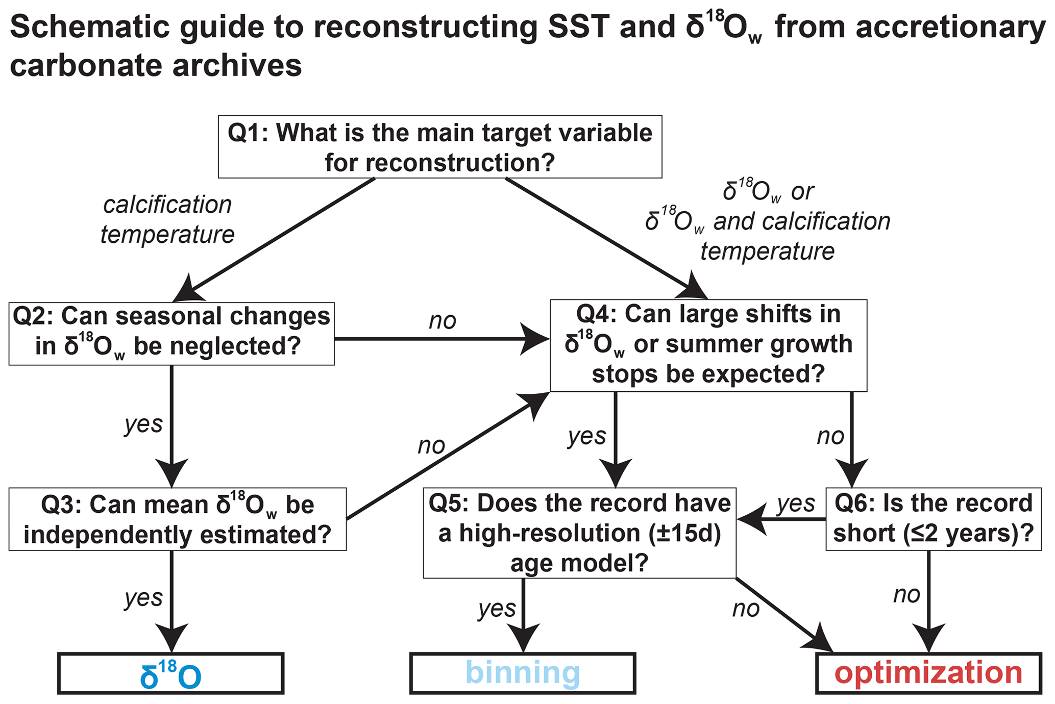
Figure 14Schematic guide to choosing the right approach for reconstructing annual mean or seasonality in SST and δ18Ow from accretionary carbonate archives. Recommendations are based on the results of testing all four approaches on the entire range of cases. Researchers can follow the six steps (questions Q1–6) to decide on the right approach for reconstructing the target variable. Guidelines are based on maximizing both accuracy and precision (see details in Supplement Data S9). Note that the smoothing approach is never the best choice. The choice between the two remaining Δ47-based approaches (binning and optimization) relies heavily on the situation and may be driven by a preference for more accurate or more precise results.
4.3 Implications for clumped isotope sample size
The optimization technique for grouping Δ47 aliquots for accurate SST and δ18Ow reconstructions allows us to assess the limitations of the clumped isotope thermometer for temperature reconstructions from high-resolution carbonate archives. The optimal sample size given by the approach is different for different cases and depends on the temporal sampling resolution and the characteristics of the record (see Supplement Data S4). As expected, in cases more like the ideal case (case 1), optimal sample sizes are low (∼14–24), while sample sizes increase in more complicated cases based on simulated natural environments (cases 14–18) or cases based on actual SST and SSS data (cases 30–33). More confined SST seasonality (cases 19–21) also requires larger samples to reconstruct (up to 100 samples in some cases). This is not surprising because variability within samples will increase in records in which the seasonality is smaller or more obscured by other environmental variability. The optimal sample size between cases and sampling resolutions is not normally distributed but tails towards high sample sizes with some extreme outliers (Shapiro–Wilk test p≪0.05; Supplement Data S10). The median sample size of all our simulations is 17 aliquots. This number lies between the minimum number of 14 ∼100 µg replicates of standards calculated by Fernandez et al. (2017) and the minimum of 20–40 ∼100 µg aliquots required for optimal paleoseasonality reconstruction from fossil bivalves by de Winter et al. (2021). This is to be expected since many of the cases explored in this study represent ideal cases compared with the natural situation. However, in these virtual cases a measure of random sub-annual variability in SST and δ18Ow was added (see Fig. 4 and Supplement Data S2), simulating a more realistic environment and resulting in poorer precision than replicates of a carbonate standard (as in Fernandez et al., 2017). Our simulations show that the optimum number of samples to be combined in seasonality studies depends on both the analytical uncertainty of Δ47 measurements (as represented by the estimate in Fernandez et al., 2017) and the variability between aliquots pooled within a sample that is attributed to actual variability within the record (as represented by our simulations and the estimate in de Winter et al., 2021). The optimal sample size is therefore a good measure for the limitations of temperature variability that can be resolved in a record and can help researchers decide which strategy to apply for combining measurements to obtain the most reliable paleoseasonality estimates or to decide whether extra sampling is required, even if the chosen approach is not to use the optimization routine itself. Note that the optimum sample size is kept equal for summer and winter samples in this study and that the optimization approach can likely achieve better performance by considering unequal sample sizes in opposite seasons (see Sect. 4.1.3 and 4.2.2). While this added flexibility comes at a higher computational cost due to the increased number of possible sample size combinations to be considered, future studies should investigate whether this updated optimization approach could yield more reliable seasonality reconstructions.
4.4 Implications for other sample size problems
While the discussion above focuses on optimizing approaches for combining samples for clumped isotope analyses in paleoseasonality reconstructions, the problem of combining samples to reduce uncertainty and isolate variation in datasets is very common (e.g., Zhang et al., 2004; Merz and Thieken, 2005; Tsukakoshi, 2011). Therefore, the approaches outlined and tested in this study have applications beyond paleoseasonality reconstructions. Examples of other problems that could benefit from applying similar approaches for reducing the uncertainty of estimates of target variables while minimizing the number of analyses required to meet analytical requirements include (1) reconstructing paleoenvironmental variability in the terrestrial realm from tooth bioapatite (e.g., Passey and Cerling, 2002; Kohn, 2004; Van Dam and Reichart, 2009; de Winter et al., 2016), (2) quantitative time series analysis of orbital cycles in stratigraphic records (e.g., Lourens et al., 2010; de Vleeschouwer et al., 2017; Noorbergen et al., 2018; Westerhold et al., 2020), (3) strontium isotope dating (e.g., McArthur et al., 2012; de Winter et al., 2020b), (4) reconstructing sub-seasonal variability from ultrahigh-resolution records (e.g., from fast-growing mollusks and gastropods; Sano et al., 2012; Warter and Müller, 2017; de Winter et al., 2020a; Yan et al., 2020), and (5) reconstructing sea surface and deep-sea temperatures across short-lived (10–100 kyr) episodes of climate change or climate shifts from deep marine archives characterized by low sedimentation rates (e.g., Lear et al., 2008; Jenkyns, 2010; Stap et al., 2010; Lauretano et al., 2018). A more detailed discussion of the implications for other sample size problems is provided in the Supplement.
The performance of three Δ47-based approaches to reconstruct seasonality from accretionary carbonate archives was evaluated in comparison with conventional δ18Oc-based reconstructions in a wide range of case studies. From the results, we conclude that while δ18Oc-based reconstructions (δ18O) yield superior precision for SST reconstructions, this method runs a high risk of yielding inaccurate results due to innate assumptions about the value of δ18Ow, which must be estimated and assumed constant year-round. Unless δ18Ow can be independently constrained or variability in δ18Ow can be neglected, Δ47-based reconstructions should be the method of choice for absolute mean annual temperature and SST seasonality reconstructions. Various techniques for combining Δ47 data were evaluated. Our findings suggest that smoothing Δ47 data using a moving average almost always results in a dampening of the seasonal cycle, which severely hampers recovery of seasonality. Applying the smoothing approach results in inaccuracies in reconstructions of MAT as well, especially in cases in which part of the seasonal cycle is obscured by variability in growth rate or multi-annual trends. More reliable seasonality reconstructions are achieved with two approaches for combining Δ47 data using time binning (binning) or applying a flexible sample size optimization (optimization) approach. Of these two approaches, optimization achieves better precision and can resolve smaller seasonal temperature differences with confidence. However, binning is often more accurate and outperforms optimization as the most reliable approach. This is especially true in cases with growth stops or δ18Ow changes in phase with temperature seasonality (e.g., strong seasonal evaporation or freshwater influx) and in longer multi-annual time series with a reliable age model. Optimization is the better choice for shorter (<3 years) records, especially if the sampling resolution can be increased, such as in short, fast-growing climate archives.
Despite the focus on the problem of resolving seasonality in carbonate archives, the findings in this study have applications for other problems in Earth science for which sample size and sampling resolution put limits on the ability to resolve specific trends, events, and cycles from time series. While the abovementioned recommendations of the optimization and binning methods are likely valid for most studies aiming to quantify the mean and amplitude of a specific cycle or event (equivalent to MAT and SST seasonality), (dynamic) moving averages (smoothing) are expected to yield the best results in studies quantifying aperiodic trends from longer data series.
All scripts used to make the calculations described in this study are compiled in the documented R package “seasonalclumped”, which is freely available on the open-source online R database CRAN (de Winter, 2021a; https://cran.r-project.org/web/packages/seasonalclumped). Annotated R scripts used to make calculations for this study are available in the digital supplement uploaded to the open-source online repository Zenodo (http://www.doi.org/10.5281/zenodo.3899926; de Winter et al., 2020d).
Supplement data, figures, and tables, as well as all scripts used to do the calculations and create the virtual datasets used in this study, are deposited in the open-source online repository Zenodo (http://www.doi.org/10.5281/zenodo.3899926; de Winter et al., 2020d). Virtual datasets generated within the context of this study are also made available as data files within the R package that contains the scripts used for this study (“seasonalclumped”; de Winter, 2021a; see https://cran.r-project.org/web/packages/seasonalclumped).
The supplement related to this article is available online at: https://doi.org/10.5194/cp-17-1315-2021-supplement.
NJdW designed the study, wrote the scripts for all calculations, and created a first draft of the paper text and figures. MZ, TA, and NJdW worked together from the first draft towards the final paper. All authors contributed to the representation of the data and methods in figures and to the discussion of the implications of the data.
The authors have no potential conflicts of interest to declare with regards to this study.
The authors would like to thank editor Alberto Reyes for his helpful suggestions for improving the paper and for moderating the review process. Thanks to Andrew Johnson and two anonymous reviewers for their comments, which helped improve the paper. All members of the Clumped Isotope research group at Utrecht University, most notably Ilja Kocken and Inigo Müller, are acknowledged for their comments and recommendations on a presentation of the initial results of this study.
This research has been supported by the European Commission, Horizon 2020 (UNBIAS (grant no. 843011)).
This paper was edited by Alberto Reyes and reviewed by Andrew Johnson and two anonymous referees.
Bahr, K. D., Jokiel, P. L., and Rodgers, K. S.: Seasonal and annual calcification rates of the Hawaiian reef coral, Montipora capitata, under present and future climate change scenarios, ICES J. Mar. Sci., 74, 1083–1091, https://doi.org/10.1093/icesjms/fsw078, 2017.
Bernasconi, S. M., Müller, I. A., Bergmann, K. D., Breitenbach, S. F., Fernandez, A., Hodell, D. A., Jaggi, M., Meckler, A. N., Millan, I., and Ziegler, M.: Reducing uncertainties in carbonate clumped isotope analysis through consistent carbonate-based standardization, Geochemistry, Geophysics, Geosystems, 19, 2895–2914, 2018.
Boutin, J., Vergely, J.-L., Koehler, J., Rouffi, F., and Reul, N.: ESA Sea Surface Salinity Climate Change Initiative (Sea_Surface_Salinity_cci): Weekly Sea Surface Salinity product v1.8, Centre for Environmental Data Analysis, available at: https://catalogue.ceda.ac.uk/uuid/e5666094722c4ca787e323a9585b0a92 (last access: 10 June 2021), 2019.
Brand, W. A., Coplen, T. B., Vogl, J., Rosner, M., and Prohaska, T.: Assessment of international reference materials for isotope-ratio analysis (IUPAC Technical Report), Pure Appl. Chem., 86, 425–467, https://doi.org/10.1515/pac-2013-1023, 2014.
Briard, J., Pucéat, E., Vennin, E., Daëron, M., Chavagnac, V., Jaillet, R., Merle, D., and de Rafélis, M.: Seawater paleotemperature and paleosalinity evolution in neritic environments of the Mediterranean margin: Insights from isotope analysis of bivalve shells, Palaeogeogr. Palaeocl., 543, 109582, https://doi.org/10.1016/j.palaeo.2019.109582, 2020.
Bowen, G. J.: WaterIsotopes.org, available at: http://wateriso.utah.edu/waterisotopes/index.html, last access: 28 July 2020.
Caldarescu, D. E., Sadatzki, H., Andersson, C., Schäfer, P., Fortunato, H., and Meckler, A. N.: Clumped isotope thermometry in bivalve shells: A tool for reconstructing seasonal upwelling, Geochim. Cosmochim. Ac., 294, 174–191, https://doi.org/10.1016/j.gca.2020.11.019, 2021.
Charles, C. D., Hunter, D. E., and Fairbanks, R. G.: Interaction between the ENSO and the Asian monsoon in a coral record of tropical climate, Science, 277, 925–928, 1997.
Comboul, M., Emile-Geay, J., Evans, M. N., Mirnateghi, N., Cobb, K. M., and Thompson, D. M.: A probabilistic model of chronological errors in layer-counted climate proxies: applications to annually banded coral archives, Clim. Past, 10, 825–841, https://doi.org/10.5194/cp-10-825-2014, 2014.
Compton, T. J., Rijkenberg, M. J. A., Drent, J., and Piersma, T.: Thermal tolerance ranges and climate variability: A comparison between bivalves from differing climates, J. Exp. Mar. Biol. Ecol., 352, 200–211, https://doi.org/10.1016/j.jembe.2007.07.010, 2007.
Cramer, B. S., Toggweiler, J. R., Wright, J. D., Katz, M. E., and Miller, K. G.: Ocean overturning since the Late Cretaceous: Inferences from a new benthic foraminiferal isotope compilation, Paleoceanography, 24, PA4216, https://doi.org/10.1029/2008PA001683, 2009.
Crossland, C.: Seasonal variations in the rates of calcification and productivity in the coral Acropora formosa on a high-latitude reef, Mar. Ecol. Prog. Ser., 15, 135–140, https://doi.org/10.3354/meps015135, 1984.
Dattalo, P.: Determining Sample Size: Balancing Power, Precision, and Practicality, Oxford University Press, New York, USA, https://doi.org/10.1093/acprof:oso/9780195315493.001.0001, 2008.
Dayem, K. E., Molnar, P., Battisti, D. S., and Roe, G. H.: Lessons learned from oxygen isotopes in modern precipitation applied to interpretation of speleothem records of paleoclimate from eastern Asia, Earth Planet. Sc. Lett., 295, 219–230, 2010.
Denton, G. H., Alley, R. B., Comer, G. C., and Broecker, W. S.: The role of seasonality in abrupt climate change, Quaternary Sci. Rev., 24, 1159–1182, https://doi.org/10.1016/j.quascirev.2004.12.002, 2005.
De Ridder, F., de Brauwere, A., Pintelon, R., Schoukens, J., Dehairs, F., Baeyens, W., and Wilkinson, B. H.: Comment on: Paleoclimatic inference from stable isotope profiles of accretionary biogenic hardparts – a quantitative approach to the evaluation of incomplete data, by Wilkinson, B. H., Ivany, L. C., 2002, Palaeogeogr. Palaeocl. Palaeoecol. 185, 95–114, Palaeogeogr. Palaeocl., 248, 473–476, https://doi.org/10.1016/j.palaeo.2006.08.004, 2007.
De Vleeschouwer, D., Vahlenkamp, M., Crucifix, M., and Pälike, H.: Alternating Southern and Northern Hemisphere climate response to astronomical forcing during the past 35 my, Geology, 45, 375–378, 2017.
de Winter, N. J.: seasonalclumped: Toolbox for Clumped Isotope Seasonality Reconstructions, available at: https://cran.r-project.org/web/packages/seasonalclumped, last access: 4 February 2021a.
de Winter, N. J.: ShellChron 0.2.8: A new tool for constructing chronologies in accretionary carbonate archives from stable oxygen isotope profiles, Geosci. Model Dev. Discuss. [preprint], https://doi.org/10.5194/gmd-2020-401, in review, 2021b.
de Winter, N. J., Snoeck, C., and Claeys, P.: Seasonal Cyclicity in Trace Elements and Stable Isotopes of Modern Horse Enamel, PloS One, 11, e0166678, https://doi.org/10.1371/journal.pone.0166678, 2016.
de Winter, N., Sinnesael, M., Makarona, C., Vansteenberge, S., and Claeys, P.: Trace element analyses of carbonates using portable and micro-X-ray fluorescence: Performance and optimization of measurement parameters and strategies, J. Anal. Atom. Spectrom., 32, 1211–1223, https://doi.org/10.1039/C6JA00361C, 2017.
de Winter, N. J., Vellekoop, J., Vorsselmans, R., Golreihan, A., Soete, J., Petersen, S. V., Meyer, K. W., Casadio, S., Speijer, R. P., and Claeys, P.: An assessment of latest Cretaceous Pycnodonte vesicularis (Lamarck, 1806) shells as records for palaeoseasonality: a multi-proxy investigation, Clim. Past, 14, 725–749, https://doi.org/10.5194/cp-14-725-2018, 2018.
de Winter, N. J., Goderis, S., Malderen, S. J. M. V., Sinnesael, M., Vansteenberge, S., Snoeck, C., Belza, J., Vanhaecke, F., and Claeys, P.: Subdaily-Scale Chemical Variability in a Torreites Sanchezi Rudist Shell: Implications for Rudist Paleobiology and the Cretaceous Day-Night Cycle, Paleoceanography and Paleoclimatology, 35, e2019PA003723, https://doi.org/10.1029/2019PA003723, 2020a.
de Winter, N. J., Ullmann, C. V., Sørensen, A. M., Thibault, N., Goderis, S., Van Malderen, S. J. M., Snoeck, C., Goolaerts, S., Vanhaecke, F., and Claeys, P.: Shell chemistry of the boreal Campanian bivalve Rastellum diluvianum (Linnaeus, 1767) reveals temperature seasonality, growth rates and life cycle of an extinct Cretaceous oyster, Biogeosciences, 17, 2897–2922, https://doi.org/10.5194/bg-17-2897-2020, 2020b.
de Winter, N. J., Vellekoop, J., Clark, A. J., Stassen, P., Speijer, R. P., and Claeys, P.: The giant marine gastropod Campanile giganteum (Lamarck, 1804) as a high-resolution archive of seasonality in the Eocene greenhouse world, Geochemistry, Geophysics, Geosystems, 21, e2019GC008794, https://doi.org/10.1029/2019GC008794, 2020c.
de Winter, N. J., Agterhuis, T., and Ziegler, M.: Supplementary data to: “Optimizing sampling strategies in high-resolution paleoclimate records: A statistical evaluation” (Version 2.1), Zenodo, https://doi.org/10.5281/zenodo.3899926, 2020d.
de Winter, N. J., Müller, I. A., Kocken, I. J., Thibault, N., Ullmann, C. V., Farnsworth, A., Lunt, D. J., Claeys, P., and Ziegler, M.: Absolute seasonal temperature estimates from clumped isotopes in bivalve shells suggest warm and variable greenhouse climate, Commun. Earth Environ., 2, 121, https://doi.org/10.1038/s43247-021-00193-9, 2021.
Eiler, J. M.: Paleoclimate reconstruction using carbonate clumped isotope thermometry, Quaternary Sci. Rev., 30, 3575–3588, 2011.
Fairbanks, R. G., Evans, M. N., Rubenstone, J. L., Mortlock, R. A., Broad, K., Moore, M. D., and Charles, C. D.: Evaluating climate indices and their geochemical proxies measured in corals, Coral Reefs, 16, S93–S100, https://doi.org/10.1007/s003380050245, 1997.
Fernandez, A., Müller, I. A., Rodríguez-Sanz, L., van Dijk, J., Looser, N., and Bernasconi, S. M.: A reassessment of the precision of carbonate clumped isotope measurements: implications for calibrations and paleoclimate reconstructions, Geochemistry, Geophysics, Geosystems, 18, 4375–4386, 2017.
Gaspar, M. B., Ferreira, R., and Monteiro, C. C.: Growth and reproductive cycle of Donax trunculus L., (Mollusca: Bivalvia) off Faro, southern Portugal, Fish. Res., 41, 309–316, https://doi.org/10.1016/S0165-7836(99)00017-X, 1999.
Goodwin, D. H., Schöne, B. R., and Dettman, D. L.: Resolution and fidelity of oxygen isotopes as paleotemperature proxies in bivalve mollusk shells: models and observations, Palaios, 18, 110–125, 2003.
Goodwin, D. H., Paul, P., and Wissink, C. L.: MoGroFunGen: A numerical model for reconstructing intra-annual growth rates of bivalve molluscs, Palaeogeogr. Palaeocl., 276, 47–55, https://doi.org/10.1016/j.palaeo.2009.02.026, 2009.
Harwood, A. J. P., Dennis, P. F., Marca, A. D., Pilling, G. M., and Millner, R. S.: The oxygen isotope composition of water masses within the North Sea, Estuarine, Coastal and Shelf Science, 78, 353–359, https://doi.org/10.1016/j.ecss.2007.12.010, 2008.
Hendriks, I. E., Basso, L., Deudero, S., Cabanellas-Reboredo, M., and Álvarez, E.: Relative growth rates of the noble pen shell Pinna nobilis throughout ontogeny around the Balearic Islands (Western Mediterranean, Spain), J. Shellfish Res., 31, 749–756, 2012.
Henkes, G. A., Passey, B. H., Grossman, E. L., Shenton, B. J., Yancey, T. E., and Pérez-Huerta, A.: Temperature evolution and the oxygen isotope composition of Phanerozoic oceans from carbonate clumped isotope thermometry, Earth Planet. Sci. Lett., 490, 40–50, https://doi.org/10.1016/j.epsl.2018.02.001, 2018.
Hurrell, J. W.: Decadal trends in the North Atlantic Oscillation: regional temperatures and precipitation, Science, 269, 676–679, 1995.
Huybers, P. and Curry, W.: Links between annual, Milankovitch and continuum temperature variability, Nature, 441, 329–332, https://doi.org/10.1038/nature04745, 2006.
Huyghe, D., Lartaud, F., Emmanuel, L., Merle, D., and Renard, M.: Palaeogene climate evolution in the Paris Basin from oxygen stable isotope (δ18O) compositions of marine molluscs, J. Geol. Soc. London, 172, 576–587, 2015.
Huyghe, D., de Rafélis, M., Ropert, M., Mouchi, V., Emmanuel, L., Renard, M., and Lartaud, F.: New insights into oyster high-resolution hinge growth patterns, Mar. Biol., 166, 48, https://doi.org/10.1007/s00227-019-3496-2, 2019.
IPCC: IPCC, 2013: Climate Change 2013: The Physical Science Basis. Contribution of Working Group I to the Fifth Assessment Report of the Intergovernmental Panel on Climate Change, Cambridge Univ. Press, Cambridge, UK, and New York, https://doi.org/10.1017/CBO9781107415324, 1535 pp., 2013.
Ivany, L. C.: Reconstructing paleoseasonality from accretionary skeletal carbonates – challenges and opportunities, The Paleontological Society Papers, 18, 133–166, 2012.
Jaffrés, J. B. D., Shields, G. A., and Wallmann, K.: The oxygen isotope evolution of seawater: A critical review of a long-standing controversy and an improved geological water cycle model for the past 3.4 billion years, Earth-Sci. Rev., 83, 83–122, https://doi.org/10.1016/j.earscirev.2007.04.002, 2007.
Jenkyns, H. C.: Geochemistry of oceanic anoxic events, Geochemistry, Geophysics, Geosystems, 11, Q03004, https://doi.org/10.1029/2009GC002788, 2010.
Johnson, A. L. A., Valentine, A. M., Leng, M. J., Schöne, B. R., and Sloane, H. J.: Life history, environment and extinction of the scallop Carolinapecten eboreus (Conrad) In the Plio-Pleistocene of the U.S. eastern seaboard, PALAIOS, 34, 49–70, https://doi.org/10.2110/palo.2018.056, 2019.
Jones, A. M., Iacumin, P., and Young, E. D.: High-resolution δ18O analysis of tooth enamel phosphate by isotope ratio monitoring gas chromatography mass spectrometry and ultraviolet laser fluorination, Chem. Geol., 153, 241–248, https://doi.org/10.1016/S0009-2541(98)00162-4, 1999.
Judd, E. J., Wilkinson, B. H., and Ivany, L. C.: The life and time of clams: Derivation of intra-annual growth rates from high-resolution oxygen isotope profiles, Palaeogeogr. Palaeocl., 490, 70–83, 2018.
Keating-Bitonti, C. R., Ivany, L. C., Affek, H. P., Douglas, P., and Samson, S. D.: Warm, not super-hot, temperatures in the early Eocene subtropics, Geology, 39, 771–774, https://doi.org/10.1130/G32054.1, 2011.
Kele, S., Breitenbach, S. F., Capezzuoli, E., Meckler, A. N., Ziegler, M., Millan, I. M., Kluge, T., Deák, J., Hanselmann, K., and John, C. M.: Temperature dependence of oxygen-and clumped isotope fractionation in carbonates: a study of travertines and tufas in the 6–95 C temperature range, Geochim. Cosmochim. Ac., 168, 172–192, 2015.
Kim, S.-T. and O'Neil, J. R.: Equilibrium and nonequilibrium oxygen isotope effects in synthetic carbonates, Geochim. Cosmochim. Ac., 61, 3461–3475, https://doi.org/10.1016/S0016-7037(97)00169-5, 1997.
Kocken, I. J., Müller, I. A., and Ziegler, M.: Optimizing the Use of Carbonate Standards to Minimize Uncertainties in Clumped Isotope Data, Geochemistry, Geophysics, Geosystems, 20, 5565–5577, https://doi.org/10.1029/2019GC008545, 2019.
Kohn, M. J.: Comment: tooth enamel mineralization in ungulates: implications for recovering a primary isotopic time-series, by BH Passey and TE Cerling (2002), Geochim. Cosmochim. Ac., 68, 403–405, 2004.
Lauretano, V., Zachos, J. C., and Lourens, L. J.: Orbitally Paced Carbon and Deep-Sea Temperature Changes at the Peak of the Early Eocene Climatic Optimum, Paleoceanography and Paleoclimatology, 33, 1050–1065, https://doi.org/10.1029/2018PA003422, 2018.
Lear, C. H., Bailey, T. R., Pearson, P. N., Coxall, H. K., and Rosenthal, Y.: Cooling and ice growth across the Eocene-Oligocene transition, Geology, 36, 251–254, 2008.
LeGrande, A. N. and Schmidt, G. A.: Global gridded data set of the oxygen isotopic composition in seawater, Geophys. Res. Lett., 33, L12604, https://doi.org/10.1029/2006GL026011, 2006.
Lisiecki, L. E. and Raymo, M. E.: A Pliocene-Pleistocene stack of 57 globally distributed benthic δ18O records, Paleoceanography, 20, PA1003, https://doi.org/10.1029/2004PA001071, 2005.
Lourens, L. J., Becker, J., Bintanja, R., Hilgen, F. J., Tuenter, E., Van de Wal, R. S., and Ziegler, M.: Linear and non-linear response of late Neogene glacial cycles to obliquity forcing and implications for the Milankovitch theory, Quaternary Sci. Rev., 29, 352–365, 2010.
McArthur, J. M., Howarth, R. J., and Shields, G. A.: Strontium isotope stratigraphy, The Geologic Time Scale, 1, 127–144, 2012.
Meckler, A. N., Ziegler, M., Millán, M. I., Breitenbach, S. F., and Bernasconi, S. M.: Long-term performance of the Kiel carbonate device with a new correction scheme for clumped isotope measurements, Rapid Commun. Mass Sp., 28, 1705–1715, 2014.
Merz, B. and Thieken, A. H.: Separating natural and epistemic uncertainty in flood frequency analysis, J. Hydrol., 309, 114–132, 2005.
Meyers, S. R.: Cyclostratigraphy and the problem of astrochronologic testing, Earth-Sci. Rev., 190, 190–223, https://doi.org/10.1016/j.earscirev.2018.11.015, 2019.
Miyaji, T., Tanabe, K., Matsushima, Y., Sato, S., Yokoyama, Y., and Matsuzaki, H.: Response of daily and annual shell growth patterns of the intertidal bivalve Phacosoma japonicum to Holocene coastal climate change in Japan, Palaeogeogr. Palaeocl., 286, 107–120, https://doi.org/10.1016/j.palaeo.2009.11.032, 2010.
Mook, W. G.: Stable carbon and oxygen isotopes of natural waters in the Netherlands, Isotope Hydrology, 1970, 163–190, 1970.
Morgan, V. and van Ommen, T. D.: Seasonality in late-Holocene climate from ice-core records, Holocene, 7, 351–354, https://doi.org/10.1177/095968369700700312, 1997.
Mosley-Thompson, E., Thompson, L. G., Dai, J., Davis, M., and Lin, P. N.: Climate of the last 500 years: High resolution ice core records, Quaternary Sci. Rev., 12, 419–430, https://doi.org/10.1016/S0277-3791(05)80006-X, 1993.
Müller, I. A., Fernandez, A., Radke, J., van Dijk, J., Bowen, D., Schwieters, J., and Bernasconi, S. M.: Carbonate clumped isotope analyses with the long-integration dual-inlet (LIDI) workflow: scratching at the lower sample weight boundaries: LIDI as key for more precise analyses on much less carbonate material, Rapid Commun. Mass Sp., 31, 1057–1066, https://doi.org/10.1002/rcm.7878, 2017.
NOAA Physical Sciences Laboratory: Homepage, available at: https://psl.noaa.gov/, last access: 10 June 2021.
Noorbergen, L. J., Abels, H. A., Hilgen, F. J., Robson, B. E., Jong, E. de, Dekkers, M. J., Krijgsman, W., Smit, J., Collinson, M. E., and Kuiper, K. F.: Conceptual models for short-eccentricity-scale climate control on peat formation in a lower Palaeocene fluvial system, north-eastern Montana (USA), Sedimentology, 65, 775–808, https://doi.org/10.1111/sed.12405, 2018.
O'Brien, C. L., Robinson, S. A., Pancost, R. D., Sinninghe Damsté, J. S., Schouten, S., Lunt, D. J., Alsenz, H., Bornemann, A., Bottini, C., Brassell, S. C., Farnsworth, A., Forster, A., Huber, B. T., Inglis, G. N., Jenkyns, H. C., Linnert, C., Littler, K., Markwick, P., McAnena, A., Mutterlose, J., Naafs, B. D. A., Püttmann, W., Sluijs, A., van Helmond, N. A. G. M., Vellekoop, J., Wagner, T., and Wrobel, N. E.: Cretaceous sea-surface temperature evolution: Constraints from TEX 86 and planktonic foraminiferal oxygen isotopes, Earth-Sci. Rev., 172, 224–247, https://doi.org/10.1016/j.earscirev.2017.07.012, 2017.
O’Donnell, M. S. and Ignizio, D. A.: Bioclimatic predictors for supporting ecological applications in the conterminous United States, U.S. Geological Survey Data Series, 691, 10 pp., 2012.
Passey, B. H. and Cerling, T. E.: Tooth enamel mineralization in ungulates: implications for recovering a primary isotopic time-series, Geochim. Cosmochim. Ac., 66, 3225–3234, 2002.
Petersen, S. V., Tabor, C. R., Lohmann, K. C., Poulsen, C. J., Meyer, K. W., Carpenter, S. J., Erickson, J. M., Matsunaga, K. K., Smith, S. Y., and Sheldon, N. D.: Temperature and salinity of the Late Cretaceous western interior seaway, Geology, 44, 903–906, 2016.
Philander, S. G. H.: El Nino southern oscillation phenomena, Nature, 302, 295–301, 1983.
R Core Team: R: A language and environment for statistical computing. R Foundation for Statistical Computing, Vienna, Austria, available at: http://www.R-project.org/ (last access: 10 June 2021), 2013.
Rodríguez-Sanz, L., Bernasconi, S. M., Marino, G., Heslop, D., Müller, I. A., Fernandez, A., Grant, K. M., and Rohling, E. J.: Penultimate deglacial warming across the Mediterranean Sea revealed by clumped isotopes in foraminifera, Scientific Reports, 7, 16572, https://doi.org/10.1038/s41598-017-16528-6, 2017.
Rohling, E. J.: Oxygen Isotope Composition of Seawater, in: The Encyclopedia of Quaternary Science, edited by: Elias, S. A., vol. 2, Amsterdam: Elsevier, 915–922 pp., 2013.
Sano, Y., Kobayashi, S., Shirai, K., Takahata, N., Matsumoto, K., Watanabe, T., Sowa, K., and Iwai, K.: Past daily light cycle recorded in the strontium/calcium ratios of giant clam shells, Nat. Commun., 3, 761, https://doi.org/10.1038/ncomms1763, 2012.
Sato, S.: Temporal change of life-history traits in fossil bivalves: an example of Phacosoma japonicum from the Pleistocene of Japan, Palaeogeogr. Palaeocl., 154, 313–323, https://doi.org/10.1016/S0031-0182(99)00106-6, 1999.
Schmitt, J., Schneider, R., Elsig, J., Leuenberger, D., Lourantou, A., Chappellaz, J., Kohler, P., Joos, F., Stocker, T. F., Leuenberger, M., and Fischer, H.: Carbon Isotope Constraints on the Deglacial CO2 Rise from Ice Cores, Science, 336, 711–714, https://doi.org/10.1126/science.1217161, 2012.
Scholz, D. and Hoffmann, D. L.: StalAge – An algorithm designed for construction of speleothem age models, Quat. Geochronol., 6, 369–382, 2011.
Schöne, B. R.: The curse of physiology – challenges and opportunities in the interpretation of geochemical data from mollusk shells, Geo-Mar. Lett., 28, 269–285, 2008.
Schöne, B. R., Fiebig, J., Pfeiffer, M., Gleß, R., Hickson, J., Johnson, A. L., Dreyer, W., and Oschmann, W.: Climate records from a bivalved Methuselah (Arctica islandica, Mollusca; Iceland), Palaeogeogr. Palaeocl., 228, 130–148, 2005.
Schöne, B. R., Rodland, D. L., Fiebig, J., Oschmann, W., Goodwin, D., Flessa, K. W., and Dettman, D.: Reliability of multitaxon, multiproxy reconstructions of environmental conditions from accretionary biogenic skeletons, J. Geol., 114, 267–285, 2006.
Scourse, J., Richardson, C., Forsythe, G., Harris, I., Heinemeier, J., Fraser, N., Briffa, K., and Jones, P.: First cross-matched floating chronology from the marine fossil record: data from growth lines of the long-lived bivalve mollusc Arctica islandica, Holocene, 16, 967–974, https://doi.org/10.1177/0959683606hl987rp, 2006.
Sha, L., Mahata, S., Duan, P., Luz, B., Zhang, P., Baker, J., Zong, B., Ning, Y., Brahim, Y. A., Zhang, H., Edwards, R. L., and Cheng, H.: A novel application of triple oxygen isotope ratios of speleothems, Geochim. Cosmochim. Ac., 270, 360–378, https://doi.org/10.1016/j.gca.2019.12.003, 2020.
Shao, D., Mei, Y., Yang, Z., Wang, Y., Yang, W., Gao, Y., Yang, L., and Sun, L.: Holocene ENSO variability in the South China Sea recorded by high-resolution oxygen isotope records from the shells of Tridacna spp., Scientific Reports, 10, 3921, https://doi.org/10.1038/s41598-020-61013-2, 2020.
Sinnesael, M., De Vleeschouwer, D., Zeeden, C., Batenburg, S. J., Da Silva, A.-C., de Winter, N. J., Dinarès-Turell, J., Drury, A. J., Gambacorta, G., and Hilgen, F. J.: The Cyclostratigraphy Intercomparison Project (CIP): consistency, merits and pitfalls, Earth-Sci. Rev., 199, 102965, https://doi.org/10.1016/j.earscirev.2019.102965, 2019.
Stap, L., Lourens, L. J., Thomas, E., Sluijs, A., Bohaty, S., and Zachos, J. C.: High-resolution deep-sea carbon and oxygen isotope records of Eocene Thermal Maximum 2 and H2, Geology, 38, 607–610, 2010.
Steffensen, J. P., Andersen, K. K., Bigler, M., Clausen, H. B., Dahl-Jensen, D., Fischer, H., Goto-Azuma, K., Hansson, M., Johnsen, S. J., and Jouzel, J.: High-resolution Greenland ice core data show abrupt climate change happens in few years, Science, 321, 680–684, 2008.
Steuber, T., Rauch, M., Masse, J.-P., Graaf, J., and Malkoč, M.: Low-latitude seasonality of Cretaceous temperatures in warm and cold episodes, Nature, 437, 1341–1344, https://doi.org/10.1038/nature04096, 2005.
Surge, D., Lohmann, K. C., and Dettman, D. L.: Controls on isotopic chemistry of the American oyster, Crassostrea virginica: implications for growth patterns, Palaeogeogr. Palaeocl., 172, 283–296, 2001.
Tagliavento, M., John, C. M., and Stemmerik, L.: Tropical temperature in the Maastrichtian Danish Basin: Data from coccolith Δ47 and δ18O, 47, 1074–1078, 2019.
Titschack, J., Zuschin, M., Spötl, C., and Baal, C.: The giant oyster Hyotissa hyotis from the northern Red Sea as a decadal-scale archive for seasonal environmental fluctuations in coral reef habitats, Coral Reefs, 29, 1061–1075, 2010.
Treble, P., Shelley, J. M. G., and Chappell, J.: Comparison of high resolution sub-annual records of trace elements in a modern (1911–1992) speleothem with instrumental climate data from southwest Australia, Earth Planet. Sc. Lett., 216, 141–153, https://doi.org/10.1016/S0012-821X(03)00504-1, 2003.
Tsukakoshi, Y.: Sampling variability and uncertainty in total diet studies, Analyst, 136, 533–539, https://doi.org/10.1039/C0AN00397B, 2011.
Tudhope, A. W.: Variability in the El Nino-Southern Oscillation Through a Glacial-Interglacial Cycle, Science, 291, 1511–1517, https://doi.org/10.1126/science.1057969, 2001.
Ullmann, C. V., Wiechert, U., and Korte, C.: Oxygen isotope fluctuations in a modern North Sea oyster (Crassostrea gigas) compared with annual variations in seawater temperature: Implications for palaeoclimate studies, Chem. Geol., 277, 160–166, 2010.
van Dam, J. A. and Reichart, G. J.: Oxygen and carbon isotope signatures in late Neogene horse teeth from Spain and application as temperature and seasonality proxies, Palaeogeogr. Palaeocl., 274, 64–81, https://doi.org/10.1016/j.palaeo.2008.12.022, 2009.
Van Rampelbergh, M., Verheyden, S., Allan, M., Quinif, Y., Keppens, E., and Claeys, P.: Monitoring of a fast-growing speleothem site from the Han-sur-Lesse cave, Belgium, indicates equilibrium deposition of the seasonal δ18O and δ13C signals in the calcite, Clim. Past, 10, 1871–1885, https://doi.org/10.5194/cp-10-1871-2014, 2014.
Vansteenberge, S., Verheyden, S., Cheng, H., Edwards, R. L., Keppens, E., and Claeys, P.: Paleoclimate in continental northwestern Europe during the Eemian and early Weichselian (125–97 ka): insights from a Belgian speleothem, Clim. Past, 12, 1445–1458, https://doi.org/10.5194/cp-12-1445-2016, 2016.
Vansteenberge, S., de Winter, N. J., Sinnesael, M., Verheyden, S., Goderis, S., Van Malderen, S. J. M., Vanhaecke, F., and Claeys, P.: Reconstructing seasonality through stable-isotope and trace-element analyses of the Proserpine stalagmite, Han-sur-Lesse cave, Belgium: indications for climate-driven changes during the last 400 years, Clim. Past, 16, 141–160, https://doi.org/10.5194/cp-16-141-2020, 2020.
Veizer, J. and Prokoph, A.: Temperatures and oxygen isotopic composition of Phanerozoic oceans, Earth-Sci. Rev., 146, 92–104, https://doi.org/10.1016/j.earscirev.2015.03.008, 2015.
Vleeschouwer, D. D., Vahlenkamp, M., Crucifix, M., and Pälike, H.: Alternating Southern and Northern Hemisphere climate response to astronomical forcing during the past 35 m.y., Geology, 45, 375–378, https://doi.org/10.1130/G38663.1, 2017.
Warter, V. and Müller, W.: Daily growth and tidal rhythms in Miocene and modern giant clams revealed via ultra-high resolution LA-ICPMS analysis – A novel methodological approach towards improved sclerochemistry, Palaeogeogr. Palaeocl., 465, 362–375, 2017.
Westerhold, T., Marwan, N., Drury, A. J., Liebrand, D., Agnini, C., Anagnostou, E., Barnet, J. S., Bohaty, S. M., De Vleeschouwer, D., and Florindo, F.: An astronomically dated record of Earth's climate and its predictability over the last 66 million years, Science, 369, 1383–1387, 2020.
Wilkinson, B. H. and Ivany, L. C.: Paleoclimatic inference from stable isotope profiles of accretionary biogenic hardparts – a quantitative approach to the evaluation of incomplete data, Palaeogeogr. Palaeocl., 185, 95–114, https://doi.org/10.1016/S0031-0182(02)00279-1, 2002.
Williams, M., Haywood, A. M., Harper, E. M., Johnson, A. L. A., Knowles, T., Leng, M. J., Lunt, D. J., Okamura, B., Taylor, P. D., and Zalasiewicz, J.: Pliocene climate and seasonality in North Atlantic shelf seas, Philos. T. Roy. Soc. A, 367, 85–108, https://doi.org/10.1098/rsta.2008.0224, 2009.
Yan, H., Liu, C., An, Z., Yang, W., Yang, Y., Huang, P., Qiu, S., Zhou, P., Zhao, N., and Fei, H.: Extreme weather events recorded by daily to hourly resolution biogeochemical proxies of marine giant clam shells, P. Natl. Acad. Sci. USA, 117, 7038–7043, https://doi.org/10.1073/pnas.1916784117, 2020.
Zhang, L., Tang, W. H., Zhang, L., and Zheng, J.: Reducing Uncertainty of Prediction from Empirical Correlations, J. Geotech. Geoenviron., 130, 526–534, https://doi.org/10.1061/(ASCE)1090-0241(2004)130:5(526), 2004.