the Creative Commons Attribution 4.0 License.
the Creative Commons Attribution 4.0 License.
 | 22 Apr 2020
Teleconnections and relationship between the El Niño–Southern Oscillation (ENSO) and the Southern Annular Mode (SAM) in reconstructions and models over the past millennium
Christoph Dätwyler
Martin Grosjean
Nathan J. Steiger
Raphael Neukom
The climate of the Southern Hemisphere (SH) is strongly influenced by variations in the El Niño–Southern Oscillation (ENSO) and the Southern Annular Mode (SAM). Because of the limited length of instrumental records in most parts of the SH, very little is known about the relationship between these two key modes of variability over time. Using proxy-based reconstructions and last-millennium climate model simulations, we find that ENSO and SAM indices are mostly negatively correlated over the past millennium. Pseudo-proxy experiments indicate that currently available proxy records are able to reliably capture ENSO–SAM relationships back to at least 1600 CE. Palaeoclimate reconstructions show mostly negative correlations back to about 1400 CE. An ensemble of last-millennium climate model simulations confirms this negative correlation, showing a stable correlation of approximately −0.3. Despite this generally negative relationship we do find intermittent periods of positive ENSO–SAM correlations in individual model simulations and in the palaeoclimate reconstructions. We do not find evidence that these relationship fluctuations are caused by exogenous forcing nor by a consistent climate pattern. However, we do find evidence that strong negative correlations are associated with strong positive (negative) anomalies in the Interdecadal Pacific Oscillation and the Amundsen Sea Low during periods when SAM and ENSO indices are of opposite (equal) sign.
- Article
(5647 KB) - Full-text XML
-
Supplement
(1533 KB) - BibTeX
- EndNote


The El Niño–Southern Oscillation (ENSO) and the Southern Annular Mode (SAM) are the Earth's and Southern Hemisphere's (SH) leading modes of interannual climate variability (Marshall, 2003; McPhaden et al., 2006), respectively. Although ENSO is a mode of tropical variability, it affects regional temperature and hydroclimate far into the mid-latitudes (Kiladis and Diaz, 1989; Cole and Cook, 1998; Moron and Ward, 1998; McCabe and Dettinger, 1999; Gouirand and Moron, 2003; Mariotti et al., 2005; Brönnimann et al., 2007), and some studies have even identified its influence in the Antarctic domain (Vance et al., 2012; Roberts et al., 2015; Jones et al., 2016; Mayewski et al., 2017). SAM is the dominant mode of SH high-latitude atmospheric variability, but its fluctuations affect climate also northwards into the subtropics, mainly by changing precipitation patterns (Silvestri and Vera, 2003; Gillett et al., 2006; Hendon et al., 2007; Risbey et al., 2009). Despite the prominent role of these two modes in driving regional SH climate, little is known about the interplay between them (Ribera and Mann, 2003; Silvestri and Vera, 2003; Carvalho et al., 2005; Fogt and Bromwich, 2006; L'Heureux and Thompson, 2006; Cai et al., 2010; Gong et al., 2010; Pohl et al., 2010; Fogt et al., 2011; Clem and Fogt, 2013; Lim et al., 2013; Yu et al., 2015; Kim et al., 2017). This interplay and its stability over time are, however, key factors for understanding tropical–extratropical teleconnections in the SH. Understanding SH climate dynamics and identifying the key drivers of interannual to multi-decadal variability requires long-term quantifications of these dominant modes of variability.
The evolution of the tropical to extratropical teleconnections between ENSO and SAM prior to the mid-20th century is unclear. The main cause for this knowledge gap is the low spatio-temporal coverage of instrumental observations across vast parts of the SH. Reliable and consistent instrumental quantifications of the SAM only extend back to the start of the satellite era in 1979 (Ho et al., 2012). Station-based indices extend back to 1957. In the instrumental indices during the most recent decades we see a significant negative correlation between the commonly used indices representing these two modes of climate variability (L'Heureux and Thompson, 2006; Wang and Cai, 2013; Kim et al., 2017). A negative correlation arises when a change in ENSO towards more El Niño-like (La Niña-like) conditions coincides with a shift in the SAM towards a more negative (positive) phase, which is associated with a shift in the storm tracks towards the Equator (South Pole) resulting in weaker (stronger) circumpolar westerly winds (e.g. Jones et al., 2009). A relationship between ENSO and SAM has been found in various studies and with a focus on different geographic regions (Ribera and Mann, 2003; Silvestri and Vera, 2003; Carvalho et al., 2005; Fogt and Bromwich, 2006; L'Heureux and Thompson, 2006; Cai et al., 2010; Gong et al., 2010; Pohl et al., 2010; Fogt et al., 2011; Clem and Fogt, 2013; Lim et al., 2013; Yu et al., 2015; Kim et al., 2017). However, they mainly rely on reanalysis data and hence only consider (parts of) the instrumental period and satellite era. Many of these studies also find a negative relationship between ENSO and SAM as seen in the instrumental indices over the last 50 years (Carvalho et al., 2005; L'Heureux and Thompson, 2006; Cai et al., 2010; Gong et al., 2010; Pohl et al., 2010; Fogt et al., 2011; Ding et al., 2012; Wang and Cai, 2013; Kim et al., 2017). But different ENSO–SAM teleconnections and changes thereof at various time periods have also been detected (Fogt and Bromwich, 2006; Clem and Fogt, 2013; Yu et al., 2015).
While there is some literature about the stability of the individual ENSO and SAM indices over the past centuries (e.g. Wilson et al., 2010; Villalba et al., 2012; Dätwyler et al., 2018, 2019) and their driving factors (e.g. Dong et al., 2018), hardly any studies exist that use palaeoclimate evidence to investigate the relationship between these modes of climate variability back in time. A study based on palaeoclimate records by Gomez et al. (2011) found a waxing and waning relationship between ENSO and SAM on century- to millennium-long timescales. Abram et al. (2014) found a significant negative correlation between their SAM reconstruction and the sea surface temperature (SST) reconstruction in the Niño3.4 region of Emile-Geay et al. (2013) since 1150 CE. However, to our knowledge, there are no studies based on annually resolved palaeoclimate data that assess the relationship between ENSO and SAM over the last millennium on sub-centennial timescales. Hence, little is still known about the tropical to extratropical teleconnections established by ENSO and SAM over this time period. Also, it is not known if the interplay between these indices exhibits long-term fluctuations and if these are driven by external forcing or internal variability, for instance via multi-decadal modes of variability such as the Interdecadal Pacific Oscillation (IPO; Folland et al., 1999; Power et al., 1999; Henley, 2017).
The literature generally speaks for a driving influence of ENSO on SAM (e.g. Ribera and Mann, 2003; Carvalho et al., 2005; Fogt and Bromwich, 2006; L'Heureux and Thompson, 2006; Cai et al., 2010; Gong et al., 2010; Yu et al., 2015; Kim et al., 2017). Carvalho et al. (2005) propose that low-frequency variability in central Pacific SSTs modulating tropical convection patterns leads to variations in the SAM. Yu et al. (2015) describe an influence of ENSO on SAM through both “an eddy-mean flow interaction mechanism and a stratospheric pathway mechanism”. Fogt et al. (2011) and Kim et al. (2017) find that influence of ENSO on SAM is linked to eddy momentum flux and associated wave propagation. Since both modes of climate variability play an important role for SH climate, a better long-term understanding of the ENSO–SAM teleconnections will lead to more precise predictions of present and future climate patterns across the SH. However, an interpretation of underlying dynamical processes will be subject to future research and is beyond the scope of this study.
Climate models can help to identify driving factors of climatic variability and teleconnection changes. Also, they have been used to test stationarity assumptions in reconstructions (e.g. Clark and Fogt, 2019). In a model environment, climate indices can be analysed over much longer periods than is possible with reanalysis data or using only instrumental measurements. Palaeoclimate reconstructions can then serve as a benchmark against which such analyses can be tested. Climate models rely on physically self-consistent processes and generate data that spatially cover the entire Earth's surface. These two characteristics provide the basis for pseudo-proxy experiments (PPEs; Mann and Rutherford, 2002; Smerdon, 2012). Pseudo-proxies are the virtual equivalents of real-world proxy records in climate models. The reliability and robustness of reconstructions that are obtained using real proxy records can be evaluated by comparing them to reconstructions based on pseudo-proxies. In addition, pseudo-proxy-based reconstructions have the advantage that they can be compared to the simulated climate, the “model truth”, over the entire reconstruction period, not only the short overlap period with instrumental data as in the real-world situation.
With this study we aim to put the observed relationship between ENSO and SAM over the most recent decades into a long-term context. We investigate how well proxy-based ENSO and SAM reconstructions can reproduce the ENSO–SAM correlation pattern. These goals are achieved by combining the knowledge on the two climate modes over the instrumental period with palaeoclimate evidence from various proxy archives and complementing this information with knowledge of climate model runs over the past millennium. In a first step, we analyse the ENSO–SAM relationship with millennium-long reconstructions that are based on real-world proxy records. In a second step, this relationship is tested with model-based indices, which in addition helps disentangle possible effects of volcanic or solar forcing from internally driven variability. Thirdly, we carry out PPEs, which serve to test whether reconstruction methods, decreasing data availability and quality back in time (i.e. proxy-inherent noise), influence or bias the reconstructed relationship between the two climate modes. Whereas an assessment and interpretation of underlying dynamical processes in the climate system are beyond the scope of this study, we provide first basic insights into spatial patterns of climate. Spatial patterns during periods of particularly strong negative or reversed positive ENSO–SAM relationships are analysed in the model world to identify potential driving factors of SH teleconnection changes.
2.1 Data
Our model analyses are based on the Community Earth System Model-Last Millennium Ensemble (CESM-LME; Otto-Bliesner et al., 2016) from which we use the sea surface temperature (SST) and sea level pressure (SLP) variables. The ensemble consists of 13 fully forced runs covering the years 850–2005 CE and one pre-industrial control run of the same length. For our analyses we only use the data from 1000 to 2005. The volcanic forcing in the CESM model is adopted from Gao et al. (2008) and the solar forcing uses Vieira et al. (2011). The values of the forcings are nominally adjusted forcings (W m−2) at the top of the atmosphere (TOA). The baseline for the total solar irradiance (TSI) is the Physikalisch-Meteorologisches Observatorium Davos (PMOD) composite over 1976–2006 (details see Schmidt et al., 2011).
As an instrumental index for ENSO, we use the Niño3.4 index based on the Extended Reconstruction Sea Surface Temperature Version 4 (ERSSTv4) instrumental dataset (Huang et al., 2015). It is defined as the area average SST anomaly from 5∘ N to 5∘ S and 170 to 120∘ W (Barnston et al., 1997).
For SAM, the Marshall (Marshall, 2003) and Fogt (Fogt et al., 2009; accessible through http://polarmet.osu.edu/ACD/sam/sam_recon.html, last access: 15 April 2020) indices are used. To calculate the model SAM index we use the definition of Gong and Wang (1999), who define it as the normalised zonal mean SLP difference between 40 and 65∘ S.
2.2 Methods
We consider data quality to be sufficiently good post-1900 and hence use 31-year running correlations between the instrumental indices back to 1915 (middle year, i.e. corresponding to the first 31-year period ranging from 1900 to 1930). Additionally, the post-1900 period covers the calibration intervals that were used for the ENSO and SAM reconstructions (1930–1990 and 1905–2005).
2.2.1 Reconstructions
This study uses the newest available ENSO and SAM reconstructions. For the SAM this is the austral summer season SAM reconstruction of Dätwyler et al. (2018). It uses the proxy records from Villalba et al. (2012), Abram et al. (2014), Neukom et al. (2014), PAGES 2k Consortium (2017) and Stenni et al. (2017) and is based on the nested ensemble-based composite-plus-scaling (CPS) method (Neukom et al., 2014).
In the case of ENSO, the palaeoclimate reconstruction is taken from Dätwyler et al. (2019) but adapted to the austral summer season December to February (DJF; Fig. S1 in the Supplement). That is, the sub-annually resolved proxy records (corals) were averaged over the 3-month interval DJF. The proxy data combine the PAGES 2k global temperature database (PAGES 2k Consortium, 2017), the SH proxy records from Neukom et al. (2014), the Antarctic ice core isotopes from Stenni et al. (2017) and also ENSO-related hydroclimate records from the Northern Hemisphere (Emile-Geay et al., 2013; Henke et al., 2017). In brief, the reconstruction method is based on principal component analysis (PCA): ENSO is quantified as the first principal component (PC) of the available proxy records in each overlapping 80-year period over the last millennium (Dätwyler et al., 2019). The key advantage of this approach is that it does not require formal calibration with instrumental data and is, therefore, not prone to the assumption that the relationships within the proxy–instrumental data matrix are stable over time. The running approach allows us to capture changes in the strength of each proxy record's contribution to the first PC over time. Such changes may happen when the relationship between the proxy and target variable changes. For details we refer to the original paper (Dätwyler et al., 2019).
Although both reconstructions share some input proxy data, they are mostly independent (for details see Sect. S2.1 in the Supplement).
To quantify the relationship between SAM and ENSO we use 31-year running correlations (for alternative window widths, see Sect. S3, Fig. S2). The significance of the running correlations between ENSO and SAM are calculated in two different ways. With the first approach, a 95 % confidence range is obtained from the uncertainties in the reconstructions. The 95 % confidence range is calculated from the running correlations of the 1000 ensemble members of the SAM and ENSO reconstructions. For the SAM reconstruction the data can be downloaded from https://www.ncdc.noaa.gov/paleo-search/study/23130 (last access: 15 April 2020). For ENSO, an ensemble for 1000 reconstructions was generated by adding noise to the reconstruction based on the residuals from the calibration with the instrumental target (Wang et al., 2014; Neukom et al., 2019; PAGES 2k Consortium, 2019). The noise is generated to have the same AR1 coefficient as the reconstruction and variance equal to the square of 2 times the augmented standard deviation of the residuals between the reconstruction and target ENSO index over the reference period 1930–1990 (SDres.aug; formula as in Dätwyler et al., 2019). With the second approach, the significant individual 31-year window correlations (p<0.05) are determined, taking lag 1 auto-correlations into account.
2.2.2 Superposed epoch analysis
Superposed epoch analysis (SEA; Haurwitz and Brier, 1981; Bradley et al., 1987; Sear et al., 1987; McGraw et al., 2016) is used to analyse whether a response to large volcanic eruptions can be detected in a time series. For comparisons with the palaeoclimate reconstructions we use the eVolv2k volcanic forcing based on Toohey and Sigl (2017) with a threshold for the aerosol optical depth (AOD) of >0.15, which selects the 13 largest eruptions in the last millennium (1109, 1171, 1230, 1257, 1286, 1345, 1458, 1600, 1641, 1695, 1784, 1809 and 1815). Model data are compared to the volcanic forcing dataset used to drive the simulations (Gao et al., 2008). We consider the 13 strongest volcanic events in the last millennium with a forcing stronger than 2.5 W m−2 (1177, 1214, 1259, 1276, 1285, 1342, 1453, 1601, 1642, 1763, 1810, 1816 and 1836). For methodological details on the SEA see Dätwyler et al. (2019).
2.2.3 Pseudo-proxy experiments
For both ENSO and SAM we calculate reconstructions based on virtual proxy records in the model world to evaluate the “real-world” reconstructions described above in Sect. 2.2.1. For all real-word proxy records that contributed to the respective reconstructions, their model-world equivalents are generated at the same geographic locations. The same reconstruction methods as were used for the real-world proxy-based reconstructions are then applied using the model ENSO and SAM indices as reconstruction targets.
We use two categories of pseudo-proxies, that is, perfect pseudo-proxies that correspond directly to the model climate variable (temperature or precipitation) that each proxy record reflects (details see Sect. S2.2) and pseudo-proxies on which noise with a certain amount and structure is imposed. Depending on the record's archive type, two different types of pseudo-proxy records are generated. Following the methodology in Steiger and Smerdon (2017), proxy-system-model (PSM) pseudo-proxies are used in the case of tree-ring width using the VS-Lite model (Tolwinski-Ward et al., 2011) based on monthly temperature and precipitation as input variables. δ18O coral records are based on a PSM with annual SST and sea surface salinity within the CESM1 simulations as input (Thompson et al., 2011). PSMs are designed to take into account specific physical and biological properties of their proxy archive. The resulting pseudo-proxies have a signal-to-noise ratio (SNR) of roughly 0.5 (Neukom et al., 2018). For other archives (e.g. ice cores, lake and marine sediments, speleothems, and historical documents) we generate statistical noise-based pseudo-proxies as described in Neukom et al. (2018). We use a signal-to-noise ratio of 0.5 by standard deviation, which is usually considered realistic for annually resolved proxy data (Wang et al., 2014) but rather conservative given the reduced correlation of local to large-scale climate in the CESM model (Neukom et al., 2018).
2.2.4 Spatial temperature and SLP patterns in models
Model temperature and SLP fields are analysed in order to identify possible spatial patterns in the climate system during periods of positive and particularly strong negative ENSO–SAM relationships. First, all years within the pre-industrial (1000–1850) period where the ENSO–SAM correlations are positive or strongly negative are selected in the 13 members of the CESM full-forced ensemble and in the pre-industrial control simulation. As a threshold for positive ENSO–SAM correlations, we use a value of 0.26, which is 3 standard deviations above the mean correlation across all datasets (−0.30). Within all 11 914 model years, this value is exceeded during 53 years (centre years of the 31-year running correlations). For negative ENSO–SAM correlations, we use a threshold of −0.67, which is 2 standard deviations below the average correlation. This threshold is exceeded during 281 years in total. Results for a symmetric choice of thresholds, i.e. 2 standard deviations above and below the average correlation, are shown in the Supplement (Figs. S6 and S7). The years during which the threshold is exceeded are divided into two subsets, depending on the state of ENSO and SAM. The first subset consists of years where SAM and ENSO are in opposite phases, i.e. either positive SAM and negative ENSO or vice versa. The second subset includes the years during which the states of SAM and ENSO are equal, that is, both either simultaneously positive or negative. We then calculate the average model temperature and SLP at each grid cell over the globe for each of these four cases individually (two cases per subset). As we are interested in anomalies relative to standard conditions, a reference pattern of positive or negative ENSO or SAM phase is subtracted for each situation. For temperature (SLP), depending on the state of ENSO (SAM), the corresponding subtracted reference pattern consists of the average model temperature (SLP) at each grid cell over all of the 11 914 model years during which ENSO (SAM) was in its positive or negative state. To avoid cancellation of circulation features in the two subsets described above, the pattern resulting from negative ENSO with positive SAM conditions is multiplied by −1 in the first subset. In the second subset, the pattern resulting from positive (negative) ENSO with positive (negative) SAM conditions is multiplied by −1 for temperature (SLP). The patterns that were multiplied by −1 were then averaged with the patterns resulting from positive ENSO with negative SAM condition and negative (positive) ENSO with negative (positive) SAM conditions. Significance is tested similarly to the SEA, by generating 1000 averages of randomly chosen years. For each of the above described four cases, the years are chosen randomly out of all model years with matching ENSO (SAM) state for temperature (SLP) and with the number of years corresponding to the number of years in the respective case. We then proceed analogously to the calculation of the climate patterns above. If these climate patterns are outside the 95 % range of the random averages, they are considered significantly higher or lower than expected by chance.
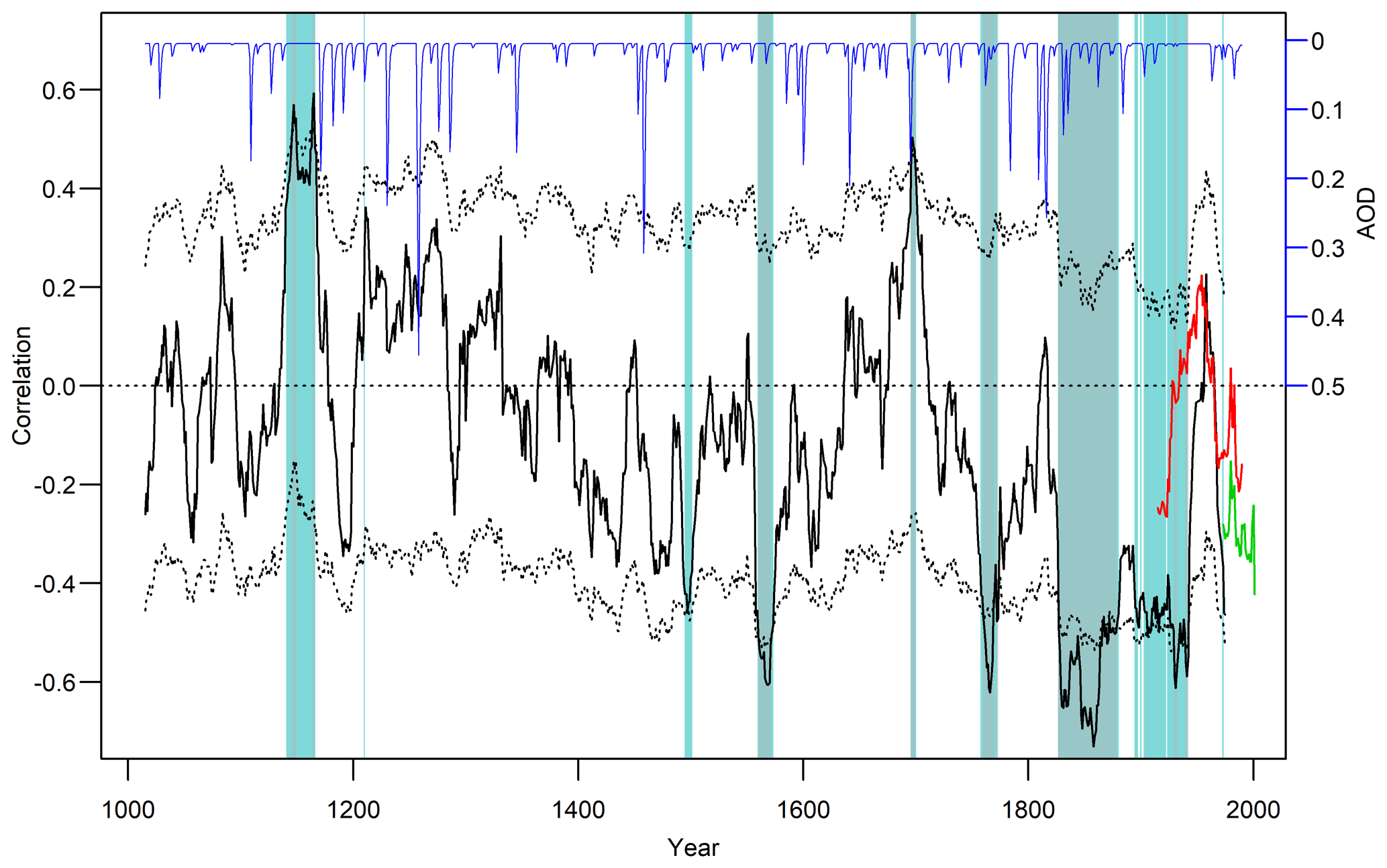
Figure 1Thirty-one-year running correlations between real-world DJF ENSO and SAM reconstructions (black) together with 31-year running correlations of the instrumental indices (red: ENSO (Niño3.4) and Fogt SAM index; green: ENSO and Marshall SAM index). For the reconstructions, the significance of the running correlations is calculated in two different ways (see Sect. 2.2.1), and values exceeding the 95 % confidence threshold are shaded with grey and cyan colour. The cyan shading corresponds to significant individual 31-year window correlations (p<0.05), taking lag 1 auto-correlation into account. The grey shading represents values that exceed the 95 % confidence range (black dotted lines) obtained from the uncertainty in the reconstructions. The volcanic forcing (Toohey and Sigl, 2017) is shown in blue. Years on the x axis reflect the middle year of the 31-year running correlations.
3.1 ENSO–SAM relationship in real-world data
The correlations between the instrumental ENSO and SAM indices are largely negative (Fig. 1), confirming results from the literature (Carvalho et al., 2005; L'Heureux and Thompson, 2006; Cai et al., 2010; Gong et al., 2010; Pohl et al., 2010; Fogt et al., 2011; Ding et al., 2012; Wang and Cai, 2013; Kim et al., 2017). Particularly during the period of high data quality back to the 1970s, the indices are significantly negatively correlated with a value of −0.38 (1980–2019). In the longer and less certain instrumental dataset (Fogt SAM index), a change in the SAM–ENSO relationship is visible around 1955.
We are confident to say that the observed negative correlations do not arise from an artefact of a specific index or choice thereof. In fact, a comparison of the correlations based on the different indices (see Sect. S4, Fig. S3) suggests that the apparent decline of the correlations between ca. 1950 and 1980 seen in our data (Fig. 1) may be an artefact of the SAM Fogt index reconstruction. Results based on the SAM Marshall index suggest that correlations were negative during the entire 20th century.
Running correlations between the real-world proxy-based austral summer ENSO and SAM reconstructions show an extension of this mostly negative relationship back to the middle of the 14th century, with the exception of a short period around 1700, where the sign of the relationship is reversed, i.e. positive (Fig. 1). Between 1150 and 1350 we see a period of mostly positive correlations, whereas during the earliest 150 years (1000–1150) generally negative correlations prevail. Over the whole millennium a trend towards more negative correlations, peaking in the 19th and 20th century, can be observed. The SEA assessing the impact of volcanic eruptions on the ENSO–SAM correlations does not yield a significant result (Fig. S4). In addition, we do not see any significant correlation between the ENSO–SAM relationship and solar forcing (not shown), indicating that fluctuations in this relationship are largely internally driven.
3.2 ENSO–SAM relationship in the CESM model
To test whether the fluctuations in the reconstructed ENSO–SAM correlations back in time and the lack of response to external forcing are realistic features or an artefact of decreasing proxy data availability and quality, we now compare the results with correlations from model simulations.
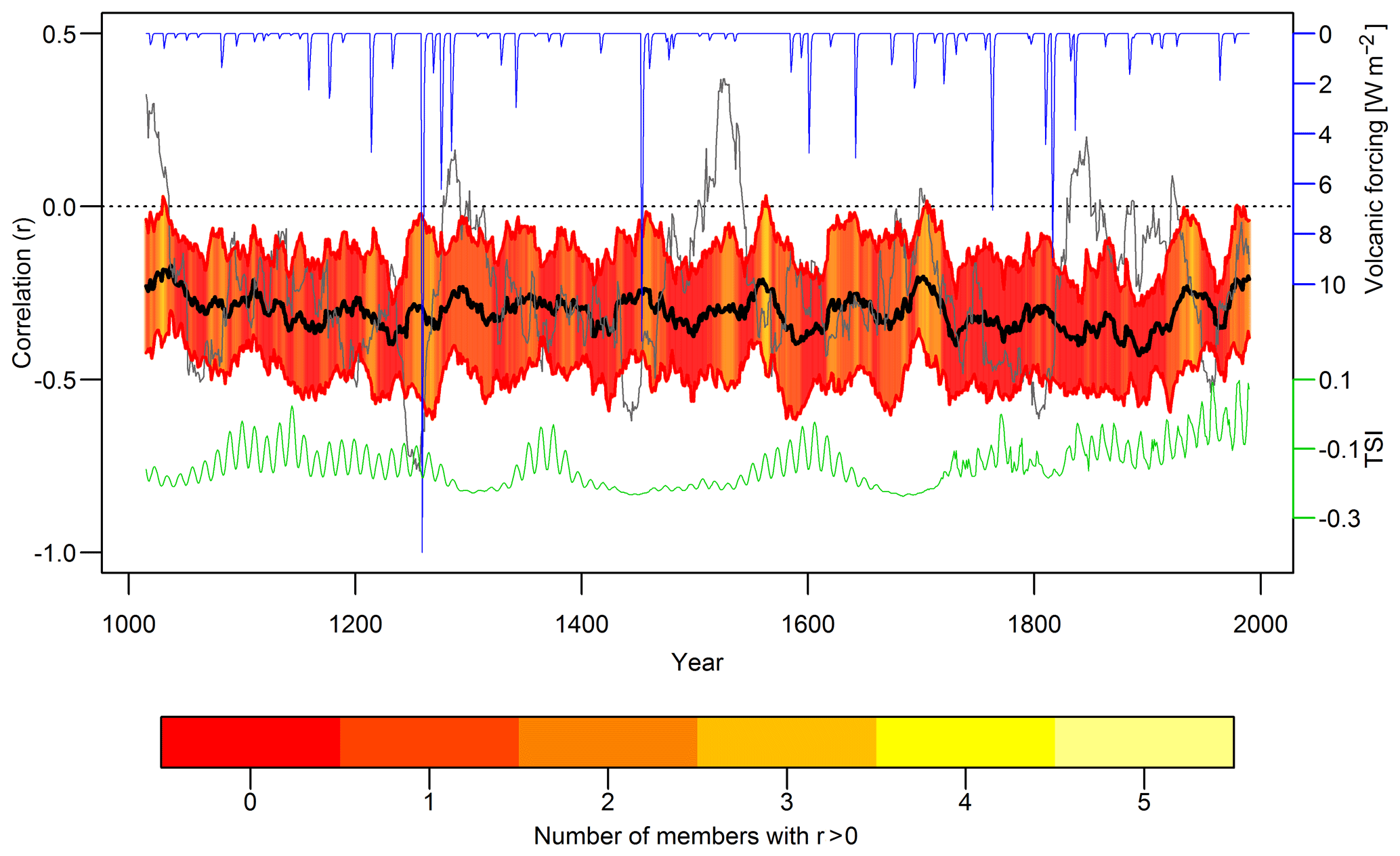
Figure 2Mean of the 31-year running correlations between model ENSO and SAM indices (models 1–13, thick black line) and ±1 standard deviation (red lines). The grey line shows the running correlations between ENSO and SAM for the control run. The volcanic forcing is shown in blue and the solar forcing in green. The red to yellow shading indicates, for each year, the number of running correlations among the individual 13 models that show a positive (reversed) sign.
The mean of the running correlations across the 13 forced simulations confirms the negative correlations in the 20th century seen in the observational datasets, indicating consistent performance of the model in simulating the ENSO–SAM relationship over this period. The ensemble mean correlations remain negative for the entire millennium with only relatively little variation (Fig. 2). In addition to this consistent average negative response, the individual 13 running correlations for each simulation also show periods with strong fluctuations in the negative correlation and intermittent changes to positive correlations (Fig. S5). However, in most of the 13 model runs, these changes are of lower magnitude compared to the palaeoproxy reconstructions. Similar to the real-world proxy-based reconstructions, the SEA of the 31-year running correlations in the individual simulations does not yield a consistent response of the ENSO–SAM relationship to volcanic eruptions (Sect. S5). There is no significant relationship between the mean running correlations of the model ENSO and SAM indices and the solar forcing (not shown). Since neither solar nor volcanic forcing appear to be driving the fluctuations in the ENSO–SAM correlations, they are likely to be caused by internal variability. This is confirmed by the pre-industrial control run, which also shows the average negative correlations, with superimposed fluctuations at multi-decadal timescales (Figs. 2 and S5).
3.3 Pseudo-proxy-based ENSO and SAM reconstructions
The general pattern of a negative correlation between ENSO and SAM and no significant influence of external forcing on this relationship is consistent among real-world proxy-based reconstructions and models, but the reconstructions show a weakening of the correlations back in time, which is not evident in the model data. To test whether the reconstructed pattern may be an artefact, we now compare our results to the pseudo-proxy experiments.
By taking the mean of all 13 running correlations between the perfect pseudo-proxy-based ENSO and SAM reconstructions we can observe that the running correlations stay negative over the whole millennium with a slight trend (originating from the reduced number of pseudo-proxy records contributing to the reconstructions back in time) towards more negative correlations towards the present (Fig. 3a). That is, we find a similar mean relationship as can be observed with the model index reconstructions, with the only difference being a slight weakening in the earliest period. This similar mean relationship also indicates that the locations and number of proxy records are suitable to capture the ENSO and SAM signals.
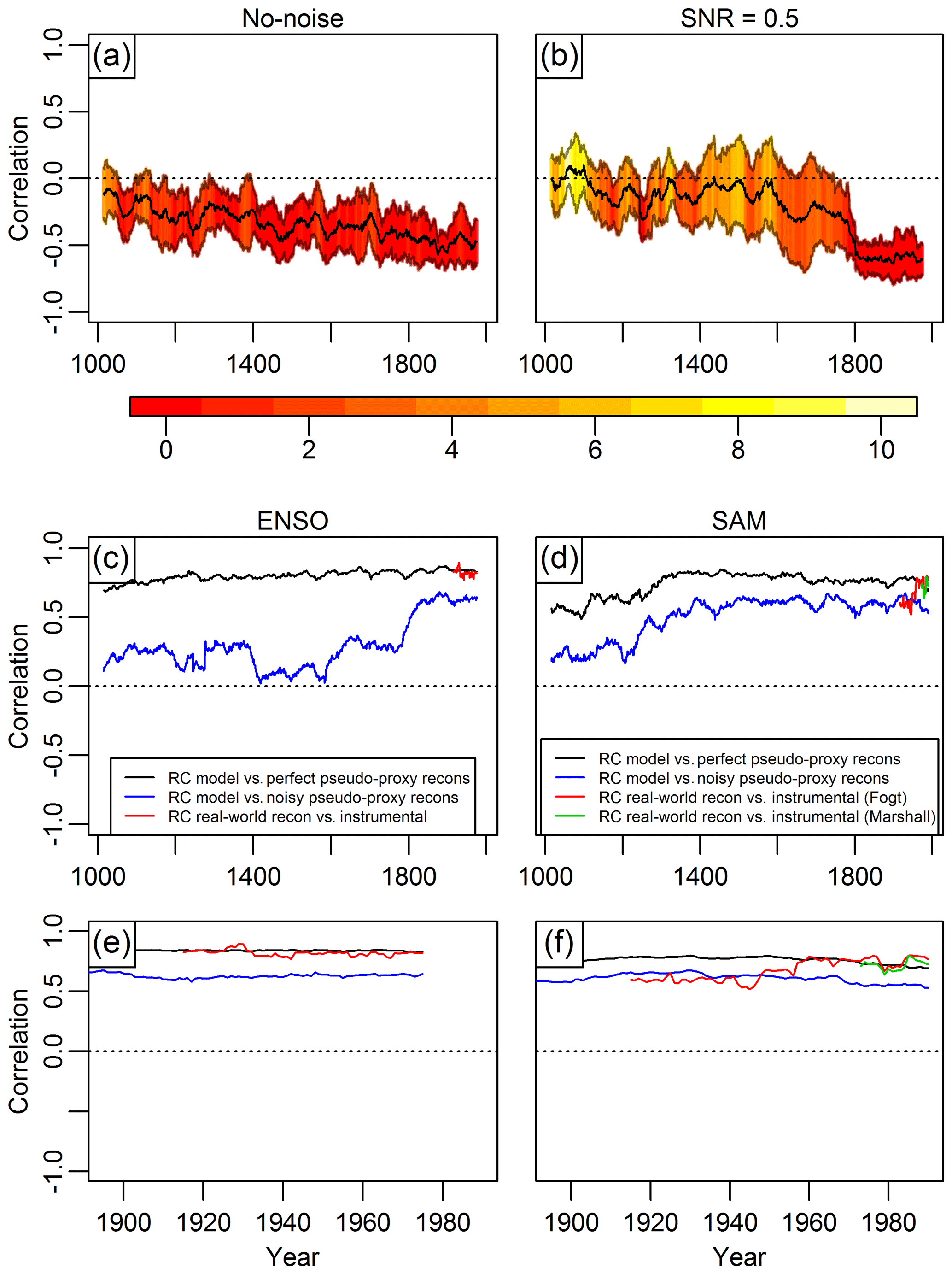
Figure 3Panel (a) shows the mean of the 31-year running correlations over all 13 models between the perfect pseudo-proxy-based ENSO and SAM reconstructions. Panel (b) shows the same as panel (a) but using the noisy pseudo-proxy-based ENSO and SAM reconstructions. The grey lines correspond to ±1 standard deviation. Panel (c) displays in black (blue) the mean 31-year running correlations over the 13 models between the model ENSO index and the perfect (noisy) pseudo-proxy-based ENSO reconstructions. The red line shows the 31-year running correlations between the real-world proxy-records-based ENSO reconstruction and the instrumental ENSO index. Panel (d) is the analogue of panel (c) but for the SAM. The red (green) line displays the 31-year running correlations between the real-world proxy-records-based SAM reconstruction and the instrumental Fogt (Marshall) SAM index. Panels (e) and (f) are enlargements of panels (c) and (d) over the 20th century. The red to yellow shading in panels (a) and (b) indicates, for each year, the number of running correlations among the individual 13 models that show a positive (reversed) sign.
To quantify the influence of noise in the proxy records, we perform additional PPEs using noisy pseudo-proxies with realistic correlations to local climate. The resulting relationship shows strong negative correlations (around −0.6) only in the 19th and 20th century (Fig. 3b). The noise in the pseudo-proxies results in weaker negative correlations pre-1600, when the number of proxy records contributing to the reconstructions decreases notably. A significant decrease in ENSO reconstruction skill prior to 1600 due to proxy availability and quality has also been seen in Dätwyler et al. (2019). The signal seen in the instrumental data over the last decades (stable negative ENSO–SAM correlations) is thus lost only partly in the perfect PPE, and the loss takes place gradually over the entire millennium. In contrast, the noisy PPE suggests that the signal decreases rapidly prior to 1800 and disappears in the pre-1600 period. This result suggests that the decreasing strength in the ENSO–SAM relationship seen in the early phase of the real-world proxy-based reconstructions may be an artefact of noise inherent in the proxy data.
The ENSO–SAM correlation in the noisy pseudo-proxy reconstructions (Fig. 3b) is slightly stronger than in the no-noise case (Fig. 3a) over 1800–2000, which is counter-intuitive. However, the difference between the two noise-levels is not significant (uncertainties overlap). The relatively strong correlations in the noisy reconstructions may also be explained by the type of noise used: as described in the Methods section (Sect. 2.2.3) and Sect. S2.2, the perfect pseudo-proxies were all only allocated to a single climate variable (either temperature or precipitation). In the case of noisy pseudo-proxies, PSMs were used for tree-ring widths and δ18O coral records. These PSMs include both temperature and precipitation or SST and salinity. We therefore hypothesise that this has led to an additional signal in the noisy pseudo-proxies, especially for the coral pseudo-proxies that, like the real-world proxies, drop out significantly prior to 1800.
The running correlations in Fig. 3c and d show the skill of the real-world and pseudo-proxy ENSO and SAM reconstructions, respectively. Note that the correlations between the reconstructions and the target can only be quantified over the instrumental period for the real-world proxy and observational data, but over the entire millennium for the PPE. In the case of perfect pseudo-proxies for both ENSO and SAM, the mean running correlations between the model index and the pseudo-proxy reconstruction remain highly positive (∼0.7–0.9) over the whole analysed period with lowest values for the SAM (∼0.5–0.6) in the 11th and 12th centuries. In the case of noisy pseudo-proxies for the ENSO, the strength of the correlations decreases significantly prior to 1800 when they remain positive but on a lower level. In the case of SAM, the noisy pseudo-proxies do not result in an equally strong decrease in the strength of the running correlations. Correlations are about 0.2 lower for the noisy PPE throughout most of the reconstruction period; only around 1300 do they start to move to levels around 0.25 between 1000 and 1200. This indicates that the SAM proxy network is more stable and representative even with fewer predictors, at least in the CESM1 model world. The performance of the real-world post-1900 reconstructions (red and green lines in Fig. 3c and d) is closer to the perfect pseudo-proxy reconstructions than to the noisy PPE. This implies that SNR =0.5 is likely to be too conservative and the case of perfect pseudo-proxies may be more representative of the real-world. This is consistent with Neukom et al. (2018), who, based on the same climate model, also showed that perfect pseudo-proxies can yield results closer to those obtained using real-world proxy records than if noisy proxies with too high a level of noise are used. A possible reason for this observation is the fact that local climate is less correlated to large-scale indices in CESM1, compared to instrumental data (Neukom et al., 2018).
Since the relationship between ENSO and SAM using perfect pseudo-proxy records resembles the relationship seen in the model truth more than when using noisy pseudo-proxies, we argue that proxy-based reconstructions can reproduce the ENSO–SAM correlation pattern in a realistic way, if there are enough proxy records contributing to the reconstructions. Even with a conservative choice in the amount of noise added to the pseudo-proxy records, a pronounced negative correlation between ENSO and SAM is observable, which further speaks for a negative relationship between ENSO and SAM. The rapid decrease in the strength of the signal in the noisy PPE prior to 1800 due to proxy noise may be over-pessimistic and the gentler decrease in the perfect PPE a more realistic representation of the real-world situation. As such, the low ENSO–SAM correlations seen in the real-world proxy-based reconstructions (Fig. 1) in the earliest few centuries of the reconstruction period are likely to be the results of the lower number and quality of proxy records.
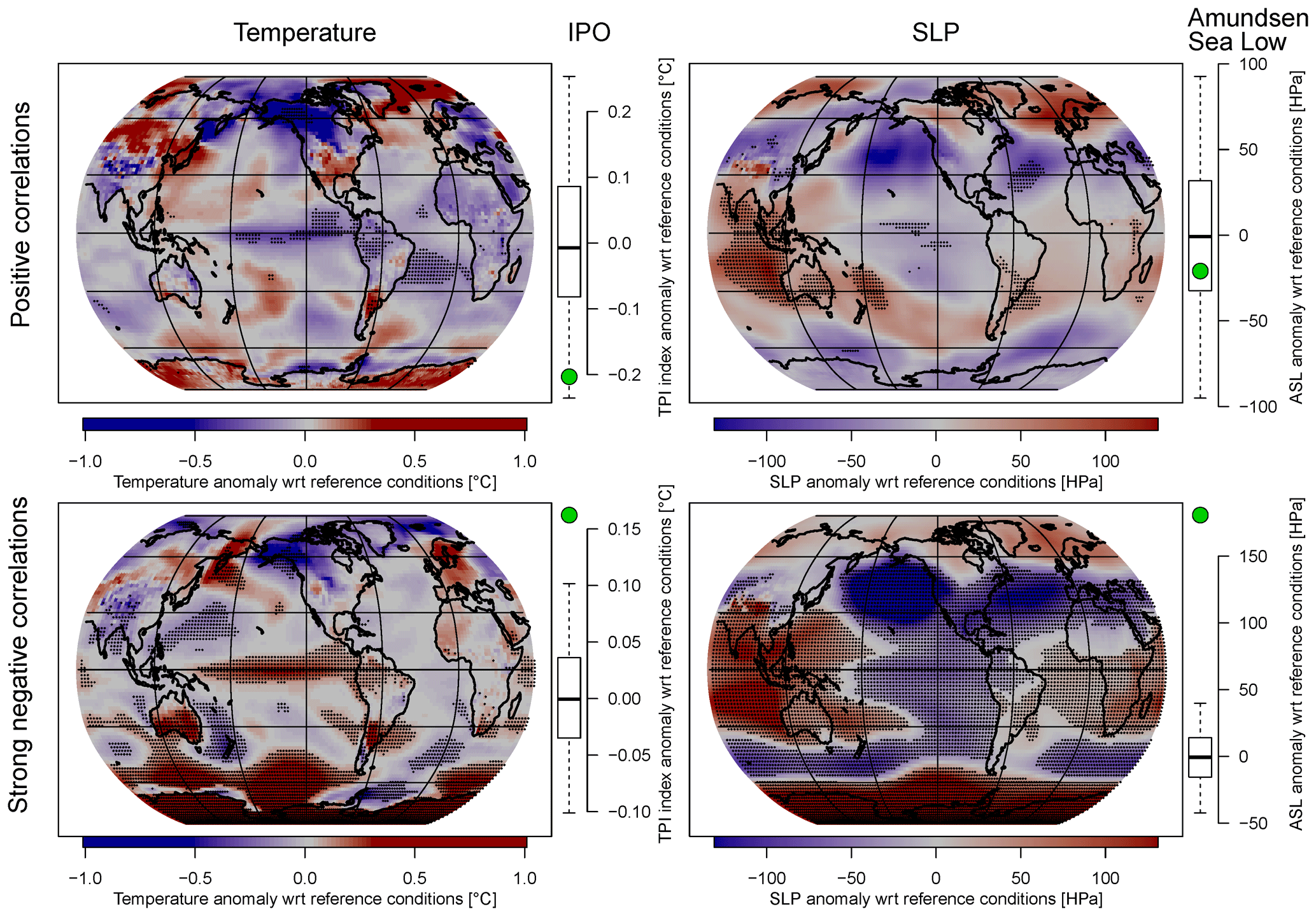
Figure 4Simulated climate anomalies during years of positive (top row) and particularly strong negative (bottom row) ENSO–SAM correlations, for which ENSO was in its positive and SAM in its negative phase or vice versa (see Methods section for details). Left maps: surface temperature anomalies. Left box-and-whisker plots: IPO anomalies. Right maps: SLP anomalies. Right box-and-whisker plots: ASL anomalies. Black stippling in the maps represents significant values. Bold lines in the boxplots represent the median of randomly sampled anomalies, boxes the interquartile range and whiskers the 95 % range. Green circles represent the average anomalies during years of positive or strong negative ENSO–SAM correlations. Note that values where ENSO is in its negative phase and SAM in its positive phase were multiplied by −1. This means that the patterns shown in the figure reflect ENSO+/SAM− conditions.

Figure 5Simulated climate anomalies during years of positive (top row) and particularly strong negative (bottom row) ENSO–SAM correlations for which ENSO and SAM were both in their positive or both in their negative phase (see Methods section for details). Left maps: surface temperature anomalies. Left box-and-whisker plots: IPO anomalies. Right maps: SLP anomalies. Right box-and-whisker plots: ASL anomalies. Black stippling in the maps represents significant values. Bold lines in the boxplots represent the median of random-sampled anomalies, boxes the interquartile range and whiskers the 95 % range. Green circles represent the average anomalies during years of positive or strong negative ENSO–SAM correlations. Note that for temperature (SLP), values where ENSO and SAM are in their negative (positive) phase were multiplied by −1. This means that in case of temperature (SLP) the patterns shown in the figure reflect ENSO+/SAM+ (ENSO−/SAM−) conditions.
In contrast, the temporal fluctuations of the correlations in the real-world reconstructions in the second half of the millennium may be real and not influenced by proxy data availability and quality. Since there was also no change in the number of proxy records contributing to the ENSO reconstruction between 1600 and 1800 and only very few dropping out in the SAM reconstruction between 1600 and 1850, a loss of key proxy records is unlikely to be responsible for, e.g., the positive swing in the ENSO–SAM relationship around 1700 or the strong negative correlations around 1765. Hence, the strong deviations towards positive correlations as seen around 1700 and the particularly strong negative correlations around 1570, 1765 and in the mid-19th century are possibly generated by internally driven teleconnection changes.
3.4 Spatial temperature and SLP patterns in the model world during periods of positive and strong negative ENSO–SAM correlations
Given that we find no significant influence of external forcing on fluctuations in the ENSO–SAM teleconnections (Sect. 3.1 and 3.2), changes in this relationship are likely internally driven. Within the last few centuries we have found periods in the real-world proxy-based reconstructions during which the sign of the ENSO–SAM correlation changes to positive. Other periods were identified where the relationship is particularly strongly negative. Are there any distinct spatial patterns in the climate system that lead to such positive or strong negative correlations? To identify such patterns, we analyse similar anomalies in the model data by averaging years where the correlations are above or below the standard deviation threshold, as described in the Methods section. The resulting temperature and SLP patterns during years of positive (top) and strong negative (bottom) ENSO–SAM correlations are shown in Figs. 4 and 5; significant anomalies are indicated with black stippling. Figure 4 includes the years during which the ENSO and SAM indices are of opposite sign, whereas Fig. 5 comprises those of equal sign.
Temperature patterns during positive ENSO–SAM correlations and when both indices are of opposite sign resemble the spatial patterns of a negative IPO (Henley, 2017; Fig. 4 top left). The average Tripole Index (TPI) is indeed negative during these years but not significantly lower than compared to random years during which ENSO was in its positive phase (Fig. 4, top left box-and-whisker plot). The corresponding temperature patterns during negative ENSO–SAM correlations exhibit a strong positive IPO fingerprint that is also reflected in the significant positive TPI (Fig. 4, bottom left). Furthermore, warmer than normal temperatures prevail towards the coast of Africa and cooler than normal temperatures are experienced in the eastern Indian Ocean. These conditions are associated with the positive phase of the Indian Ocean Dipole (IOD; Saji et al., 1999; Webster et al., 1999). When both indices are of equal sign and during positive ENSO–SAM correlations, there is no pronounced IPO pattern and the TPI is about zero (Fig. 5, top left) and slightly negative for strong negative ENSO–SAM correlations (Fig. 5, bottom left box-and-whisker plot).
For SLP the spatial anomaly patterns are shown on the right-hand side in Figs. 4 and 5, including also the anomalies of the Amundsen Sea Low (ASL) index (calculated as in Hosking et al. (2013), that is, averaged SLP over 60–70∘ S and 170∘ E–70∘ W). In the case where both ENSO and SAM are of opposite sign and during strong negative correlations, a clearly significant positive ASL anomaly goes along with a pressure pattern that is associated with negative SAM phases (Fig. 4, bottom right). The opposite holds true during strong negative ENSO–SAM correlations but when both indices are of equal sign. The SH SLP patterns resemble variations in pressure seen during positive SAM phases (Fig. 5, bottom right map), i.e. lower than usual pressure over Antarctica and higher than usual pressure across the mid-latitudes. Furthermore, a clearly significant negative ASL anomaly can be observed. During positive correlations pronounced low-pressure anomalies in the Amundsen Sea can be seen that are reflected in the negative (though not significant) ASL index (Fig. 5, top right).
Fogt and Bromwich (2006) found that when SAM and ENSO are negatively correlated, ENSO's teleconnections to the high latitudes and South Pacific are strengthened, and, conversely, they are weakened during times when SAM and ENSO are positively correlated. This result could imply that the strong anomalies we find during periods where ENSO and SAM are in opposite phases (Fig. 4, bottom row) are due to an amplified influence of ENSO up to the SH's high latitudes. In fact, these anomalies are larger and more widely significant compared to the patterns during positive ENSO–SAM correlations (Fig. 4, top row). Similarly, this can be seen in the SLP patterns in Fig. 5, where the SH high latitudes exhibit much larger anomalies and the ASL becomes significant during strong negative ENSO–SAM correlations (bottom row).
In contrast to SLP in both Figs. 4 and 5 and temperature in Fig. 4, such larger and more widely significant anomalies cannot be observed for temperature during periods when SAM and ENSO indices are of equal sign (Fig. 5, left maps). Rather the temperature patterns during positive ENSO–SAM correlations (Fig. 5, top left map) show significant cold temperature anomalies over the Amundsen and Ross seas and warm anomalies in the Bellingshausen and Weddell Sea regions, which are both less pronounced and not significant during strong negative ENSO–SAM correlations (Fig. 5, bottom left map).
Our analysis suggests that there is no single consistent temperature or SLP pattern that explains the internally driven reversal of ENSO–SAM correlations in the CESM simulations (top rows in Figs. 4 and 5).
Further in-depth analyses that are beyond the scope of this study are required to give sound interpretations of the underlying mechanism that drive the observed phenomena. Upcoming high-quality climate field reconstructions of temperature, SLP and associated climate indices will greatly help to gain a deeper understanding of the spatio-temporal relationships and the ocean–atmospheric dynamics that are involved in the interplay between ENSO and SAM.
We present, for the first time, a multi-century analysis of SH tropical–extratropical teleconnections in palaeoproxy observations and model data. The CESM1 climate model simulations confirm what we see in the instrumental indices and in proxy-based ENSO and SAM reconstructions: a generally negative correlation between the ENSO and SAM with a multi-century average around −0.3. This relationship is perturbed only by internal variability as we do not find any significant response to solar and volcanic external forcing. The relationship between ENSO and SAM as seen in the model indices agrees well with the relationship established by perfect pseudo-proxy record reconstructions, indicating that reconstruction methods and geographic distribution of the proxy records are well suited to capture the essential ENSO and SAM signal. If a significant amount of noise is added to the pseudo-proxy records, the negative correlations weaken pre-1800 and even further pre-1600, when the number of available proxy records drops below a critical threshold (∼30 proxy records), indicating reduced reliability of the reconstructed ENSO–SAM correlations during this period.
Reconstructions and model simulations show that there are repeated periods where the tropical–extratropical correlations change sign or are particularly strongly negative. We find no consistent spatial climate patterns during periods of reversed positive ENSO–SAM correlations. In contrast, possibly stronger tropical to high-latitude teleconnections are seen during periods of strong negative ENSO–SAM correlations. These periods are associated with strong positive (negative) IPO and ASL anomalies when ENSO and SAM are of opposite (equal) phase.
Our results may serve as a basis for future research studying the long-term behaviour and stability of teleconnections in the SH. This will put into a larger context observed and predicted SH climate changes, such as a potential expansion of the Hadley Cell (e.g. Hu et al., 2013) or changes in Antarctic sea-ice extent (e.g. Turner et al., 2009; Parkinson and Cavalieri, 2012).
The data relevant to this study are available at the NOAA paleoclimatology database under https://www.ncdc.noaa.gov/paleo/study/29050.
The supplement related to this article is available online at: https://doi.org/10.5194/cp-16-743-2020-supplement.
RN and CD designed the study. Data analysis was led by CD with contributions from RN. The writing was led by CD with exception of Sect. 3.4 and the abstract. Section 3.4 was jointly written by CD and RN, and the abstract was written by CD, NJS and RN. All figures were made by CD, except for Fig. 4, which was made by RN and CD. Pseudo-proxy data were provided by NJS and RN. All authors jointly discussed and contributed to the writing.
The authors declare that they have no conflict of interest.
This work partly resulted from contributions to the Past Global Changes (PAGES) 2k initiative. Members of the PAGES 2k Consortium are thanked for providing public access to proxy data and metadata. We thank two anonymous reviewers for their constructive comments that greatly helped to improve the original paper.
This research has been supported by the Swiss National Science Foundation (SNF) Ambizione (grant no. PZ00P2_154802) and the United States National Science Foundation (grant no. NSF-AGS 1805490).
This paper was edited by Elizabeth Thomas and reviewed by two anonymous referees.
Abram, N. J., Mulvaney, R., Vimeux, F., Phipps, S. J., Turner, J., and England, M. H.: Evolution of the Southern Annular Mode during the past millennium, Nat. Clim. Change, 4, 564–569, https://doi.org/10.1038/nclimate2235, 2014.
Barnston, A. G., Chelliah, M., and Goldenberg, S. B.: Documentation of a highly ENSO-related sst region in the equatorial pacific: Research note, Atmos.-Ocean, 35, 367–383, https://doi.org/10.1080/07055900.1997.9649597, 1997.
Bradley, R. S., Diaz, H. F., Kiladis, G. N., and Eischeid, J. K.: ENSO signal in continental temperature and precipitation records, Nature, 327, 497–501, https://doi.org/10.1038/327497a0, 1987.
Brönnimann, S., Xoplaki, E., Casty, C., Pauling, A., and Luterbacher, J.: ENSO influence on Europe during the last centuries, Clim. Dynam., 28, 181–197, https://doi.org/10.1007/s00382-006-0175-z, 2007.
Cai, W., Sullivan, A., and Cowan, T.: Interactions of ENSO, the IOD, and the SAM in CMIP3 Models, J. Climate, 24, 1688–1704, https://doi.org/10.1175/2010JCLI3744.1, 2010.
Carvalho, L. M. V., Jones, C., and Ambrizzi, T.: Opposite Phases of the Antarctic Oscillation and Relationships with Intraseasonal to Interannual Activity in the Tropics during the Austral Summer, J. Climate, 18, 702–718, https://doi.org/10.1175/JCLI-3284.1, 2005.
Clark, L. and Fogt, R.: Southern Hemisphere Pressure Relationships during the 20th Century – Implications for Climate Reconstructions and Model Evaluation, Geosciences, 9, 413, 2019.
Clem, K. R. and Fogt, R. L.: Varying roles of ENSO and SAM on the Antarctic Peninsula climate in austral spring, J. Geophys. Res.-Atmos., 118, 11481–11492, https://doi.org/10.1002/jgrd.50860, 2013.
Cole, J. E. and Cook, E. R.: The changing relationship between ENSO variability and moisture balance in the continental United States, Geophys. Res. Lett., 25, 4529–4532, https://doi.org/10.1029/1998GL900145, 1998.
Dätwyler, C., Neukom, R., Abram, N. J., Gallant, A. J. E., Grosjean, M., Jacques-Coper, M., Karoly, D. J., and Villalba, R.: Teleconnection stationarity, variability and trends of the Southern Annular Mode (SAM) during the last millennium, Clim. Dynam., 51, 2321–2339, https://doi.org/10.1007/s00382-017-4015-0, 2018.
Dätwyler, C., Abram, N. J., Grosjean, M., Wahl, E. R., and Neukom, R.: El Niño – Southern Oscillation variability, teleconnection changes and responses to large volcanic eruptions since AD 1000, Int. J. Climatol., 39, 2711–2724, https://doi.org/10.1002/joc.5983, 2019.
Ding, Q., Steig, E. J., Battisti, D. S., and Wallace, J. M.: Influence of the Tropics on the Southern Annular Mode, J. Climate, 25, 6330–6348, https://doi.org/10.1175/JCLI-D-11-00523.1, 2012.
Dong, B., Dai, A., Vuille, M., and Timm, O. E.: Asymmetric Modulation of ENSO Teleconnections by the Interdecadal Pacific Oscillation, J. Climate, 31, 7337–7361, https://doi.org/10.1175/JCLI-D-17-0663.1, 2018.
Emile-Geay, J., Cobb, K. M., Mann, M. E., and Wittenberg, A. T.: Estimating Central Equatorial Pacific SST Variability over the Past Millennium. Part II: Reconstructions and Implications, J. Climate, 26, 2329–2352, https://doi.org/10.1175/JCLI-D-11-00511.1, 2013.
Fogt, R. L. and Bromwich, D. H.: Decadal Variability of the ENSO Teleconnection to the High-Latitude South Pacific Governed by Coupling with the Southern Annular Mode, J. Climate, 19, 979–997, https://doi.org/10.1175/JCLI3671.1, 2006.
Fogt, R. L., Bromwich, D. H., and Hines, K. M.: Understanding the SAM influence on the South Pacific ENSO teleconnection, Clim. Dynam., 36, 1555–1576, https://doi.org/10.1007/s00382-010-0905-0, 2011.
Fogt, R. L., Perlwitz, J., Monaghan, A. J., Bromwich, D. H., Jones, J. M., and Marshall, G. J.: Historical SAM Variability. Part II: Twentieth-Century Variability and Trends from Reconstructions, Observations, and the IPCC AR4 Models, J. Climate, 22, 5346–5365, https://doi.org/10.1175/2009JCLI2786.1, 2009.
Folland, C. K., Parker, D. E., Colman, A. W., and Washington, R.: Large Scale Modes of Ocean Surface Temperature Since the Late Nineteenth Century, in: Beyond El Niño: Decadal and Interdecadal Climate Variability, edited by: Navarra, A., Springer Berlin Heidelberg, Berlin, Heidelberg, 73–102, 1999.
Gao, C., Robock, A., and Ammann, C.: Volcanic forcing of climate over the past 1500 years: An improved ice core-based index for climate models, J. Geophys. Res., 113, D23, https://doi.org/10.1029/2008JD010239, 2008.
Gillett, N. P., Kell, T. D., and Jones, P. D.: Regional climate impacts of the Southern Annular Mode, Geophys. Res. Lett., 33, 23, https://doi.org/10.1029/2006GL027721, 2006.
Gomez, B., Carter, L., Orpin, A. R., Cobb, K. M., Page, M. J., Trustrum, N. A., and Palmer, A. S.: ENSO/SAM interactions during the middle and late Holocene, The Holocene, 22, 23–30, https://doi.org/10.1177/0959683611405241, 2011.
Gong, D. and Wang, S.: Definition of Antarctic Oscillation index, Geophys. Res. Lett., 26, 459–462, https://doi.org/10.1029/1999GL900003, 1999.
Gong, T., Feldstein, S. B., and Luo, D.: The Impact of ENSO on Wave Breaking and Southern Annular Mode Events, J. Atmos. Sci., 67, 2854–2870, https://doi.org/10.1175/2010JAS3311.1, 2010.
Gouirand, I. and Moron, V.: Variability of the impact of El Niño – southern oscillation on sea-level pressure anomalies over the North Atlantic in January to March (1874–1996), Int. J. Climatol., 23, 1549–1566, https://doi.org/10.1002/joc.963, 2003.
Haurwitz, M. W. and Brier, G. W.: A Critique of the Superposed Epoch Analysis Method: Its Application to Solar–Weather Relations, Mon. Weather Rev., 109, 2074–2079, https://doi.org/10.1175/1520-0493(1981)109<2074:ACOTSE>2.0.CO;2, 1981.
Hendon, H. H., Thompson, D. W. J., and Wheeler, M. C.: Australian Rainfall and Surface Temperature Variations Associated with the Southern Hemisphere Annular Mode, J. Climate, 20, 2452–2467, https://doi.org/10.1175/JCLI4134.1, 2007.
Henke, L. M. K., Lambert, F. H., and Charman, D. J.: Was the Little Ice Age more or less El Niño-like than the Medieval Climate Anomaly? Evidence from hydrological and temperature proxy data, Clim. Past, 13, 267–301, https://doi.org/10.5194/cp-13-267-2017, 2017.
Henley, B. J.: Pacific decadal climate variability: Indices, patterns and tropical-extratropical interactions, Global Planet. Change, 155, 42–55, https://doi.org/10.1016/j.gloplacha.2017.06.004, 2017.
Ho, M., Kiem, A. S., and Verdon-Kidd, D. C.: The Southern Annular Mode: a comparison of indices, Hydrol. Earth Syst. Sci., 16, 967–982, https://doi.org/10.5194/hess-16-967-2012, 2012.
Hosking, J. S., Orr, A., Marshall, G. J., Turner, J., and Phillips, T.: The Influence of the Amundsen–Bellingshausen Seas Low on the Climate of West Antarctica and Its Representation in Coupled Climate Model Simulations, J. Climate, 26, 6633–6648, https://doi.org/10.1175/JCLI-D-12-00813.1, 2013.
Hu, Y., Tao, L., and Liu, J.: Poleward expansion of the hadley circulation in CMIP5 simulations, Adv. Atmos. Sci., 30, 790–795, https://doi.org/10.1007/s00376-012-2187-4, 2013.
Huang, B., Banzon, V. F., Freeman, E., Lawrimore, J., Liu, W., Peterson, T. C., Smith, T. M., Thorne, P. W., Woodruff, S. D., and Zhang, H.-M.: Extended Reconstructed Sea Surface Temperature (ERSST), Version 4, NOAA National Centers for Environmental Information, https://doi.org/10.7289/V5KD1VVF, 2015.
Jones, J. M., Fogt, R. L., Widmann, M., Marshall, G. J., Jones, P. D., and Visbeck, M.: Historical SAM Variability. Part I: Century-Length Seasonal Reconstructions, J. Climate, 22, 5319–5345, https://doi.org/10.1175/2009JCLI2785.1, 2009.
Jones, J. M., Gille, S. T., Goosse, H., Abram, N. J., Canziani, P. O., Charman, D. J., Clem, K. R., Crosta, X., Lavergne, C. de, Eisenman, I., England, M. H., Fogt, R. L., Frankcombe, L. M., Marshall, G. J., Masson-Delmotte, V., Morrison, A. K., Orsi, A. J., Raphael, M. N., Renwick, J. A., Schneider, D. P., Simpkins, G. R., Steig, E. J., Stenni, B., Swingedouw, D., and Vance, T. R.: Assessing recent trends in high-latitude Southern Hemisphere surface climate, Nat. Clim. Change, 6, 917–926, https://doi.org/10.1038/nclimate3103, 2016.
Kiladis, G. N. and Diaz, H. F.: Global Climatic Anomalies Associated with Extremes in the Southern Oscillation, J. Climate, 2, 1069–1090, https://doi.org/10.1175/1520-0442(1989)002<1069:GCAAWE>2.0.CO;2, 1989.
Kim, B.-M., Choi, H., Kim, S.-J., and Choi, W.: Amplitude-dependent relationship between the Southern Annular Mode and the El Niño Southern Oscillation in austral summer, Asia-Pacific J. Atmos. Sci., 53, 85–100, https://doi.org/10.1007/s13143-017-0007-6, 2017.
L'Heureux, M. L. and Thompson, D. W. J.: Observed Relationships between the El Niño – Southern Oscillation and the Extratropical Zonal-Mean Circulation, J. Climate, 19, 276–287, https://doi.org/10.1175/JCLI3617.1, 2006.
Lim, E.-P., Hendon, H. H., and Rashid, H.: Seasonal Predictability of the Southern Annular Mode due to Its Association with ENSO, J. Climate, 26, 8037–8054, https://doi.org/10.1175/JCLI-D-13-00006.1, 2013.
Mann, M. E. and Rutherford, S.: Climate reconstruction using “Pseudoproxies”, Geophys. Res. Lett., 29, 139-1–139-4, https://doi.org/10.1029/2001GL014554, 2002.
Mariotti, A., Ballabrera-Poy, J., and Zeng, N.: Tropical influence on Euro-Asian autumn rainfall variability, Clim. Dynam., 24, 511–521, https://doi.org/10.1007/s00382-004-0498-6, 2005.
Marshall, G. J.: Trends in the Southern Annular Mode from Observations and Reanalyses, J. Climate, 16, 4134–4143, https://doi.org/10.1175/1520-0442(2003)016<4134:TITSAM>2.0.CO;2, 2003.
Mayewski, P. A., Carleton, A. M., Birkel, S. D., Dixon, D., Kurbatov, A. V., Korotkikh, E., McConnell, J., Curran, M., Cole-Dai, J., Jiang, S., Plummer, C., Vance, T., Maasch, K. A., Sneed, S. B., and Handley, M.: Ice core and climate reanalysis analogs to predict Antarctic and Southern Hemisphere climate changes, Quaternary Sci. Rev., 155, 50–66, https://doi.org/10.1016/j.quascirev.2016.11.017, 2017.
McCabe, G. J. and Dettinger, M. D.: Decadal variations in the strength of ENSO teleconnections with precipitation in the western United States, Int. J. Climatol., 19, 1399–1410, https://doi.org/10.1002/(SICI)1097-0088(19991115)19:13<1399::AID-JOC457>3.0.CO;2-A, 1999.
McGraw, M. C., Barnes, E. A., and Deser, C.: Reconciling the observed and modeled Southern Hemisphere circulation response to volcanic eruptions, Geophys. Res. Lett., 43, 7259–7266, https://doi.org/10.1002/2016GL069835, 2016.
McPhaden, M. J., Zebiak, S. E., and Glantz, M. H.: ENSO as an Integrating Concept in Earth Science, Science, 314, 1740–1745, https://doi.org/10.1126/science.1132588, 2006.
Moron, V. and Ward, M. N.: ENSO teleconnections with climate variability in the European and African sectors, Weather, 53, 287–295, https://doi.org/10.1002/j.1477-8696.1998.tb06403.x, 1998.
Neukom, R., Gergis, J., Karoly, D. J., Wanner, H., Curran, M., Elbert, J., González-Rouco, F., Linsley, B. K., Moy, A. D., Mundo, I., Raible, C. C., Steig, E. J., van Ommen, T., Vance, T., Villalba, R., Zinke, J., and Frank, D.: Inter-hemispheric temperature variability over the past millennium, Nat. Clim. Change, 4, 362–367, https://doi.org/10.1038/nclimate2174, 2014.
Neukom, R., Schurer, A. P., Steiger, N. J., and Hegerl, G. C.: Possible causes of data model discrepancy in the temperature history of the last Millennium, Sci. Rep.-UK, 8, 7572, https://doi.org/10.1038/s41598-018-25862-2, 2018.
Neukom, R., Steiger, N., Gómez-Navarro, J. J., Wang, J., and Werner, J. P.: No evidence for globally coherent warm and cold periods over the preindustrial Common Era, Nature, 571, 550–554, https://doi.org/10.1038/s41586-019-1401-2, 2019.
Otto-Bliesner, B. L., Brady, E. C., Fasullo, J., Jahn, A., Landrum, L., Stevenson, S., Rosenbloom, N., Mai, A., and Strand, G.: Climate Variability and Change since 850 CE: An Ensemble Approach with the Community Earth System Model, B. Am. Meteorol. Soc., 97, 735–754, https://doi.org/10.1175/BAMS-D-14-00233.1, 2016.
PAGES 2k Consortium: A global multiproxy database for temperature reconstructions of the Common Era, Scientific data, 4, 170088, https://doi.org/10.1038/sdata.2017.88, 2017.
PAGES 2k Consortium: Consistent multidecadal variability in global temperature reconstructions and simulations over the Common Era, Nat. Geosci., 12, 643–649, https://doi.org/10.1038/s41561-019-0400-0, 2019.
Parkinson, C. L. and Cavalieri, D. J.: Antarctic sea ice variability and trends, 1979–2010, The Cryosphere, 6, 871–880, https://doi.org/10.5194/tc-6-871-2012, 2012.
Pohl, B., Fauchereau, N., Reason, C. J. C., and Rouault, M.: Relationships between the Antarctic Oscillation, the Madden–Julian Oscillation, and ENSO, and Consequences for Rainfall Analysis, J. Climate, 23, 238–254, https://doi.org/10.1175/2009JCLI2443.1, 2010.
Power, S., Casey, T., Folland, C., Colman, A., and Mehta, V.: Inter-decadal modulation of the impact of ENSO on Australia, Clim. Dynam., 15, 319–324, https://doi.org/10.1007/s003820050284, 1999.
Ribera, P. and Mann, M. E.: ENSO related variability in the Southern Hemisphere, 1948–2000, Geophys. Res. Lett., 30, 6-1–6-4, https://doi.org/10.1029/2002GL015818, 2003.
Risbey, J. S., Pook, M. J., McIntosh, P. C., Wheeler, M. C., and Hendon, H. H.: On the Remote Drivers of Rainfall Variability in Australia, Mon. Weather Rev., 137, 3233–3253, https://doi.org/10.1175/2009MWR2861.1, 2009.
Roberts, J., Plummer, C., Vance, T., van Ommen, T., Moy, A., Poynter, S., Treverrow, A., Curran, M., and George, S.: A 2000-year annual record of snow accumulation rates for Law Dome, East Antarctica, Clim. Past, 11, 697–707, https://doi.org/10.5194/cp-11-697-2015, 2015.
Saji, N. H., Goswami, B. N., Vinayachandran, P. N., and Yamagata, T.: A dipole mode in the tropical Indian Ocean, Nature, 401, 360–363, https://doi.org/10.1038/43854, 1999.
Schmidt, G. A., Jungclaus, J. H., Ammann, C. M., Bard, E., Braconnot, P., Crowley, T. J., Delaygue, G., Joos, F., Krivova, N. A., Muscheler, R., Otto-Bliesner, B. L., Pongratz, J., Shindell, D. T., Solanki, S. K., Steinhilber, F., and Vieira, L. E. A.: Climate forcing reconstructions for use in PMIP simulations of the last millennium (v1.0), Geosci. Model Dev., 4, 33–45, https://doi.org/10.5194/gmd-4-33-2011, 2011.
Sear, C. B., Kelly, P. M., Jones, P. D., and Goodess, C. M.: Global surface-temperature responses to major volcanic eruptions, Nature, 330, 365–367, https://doi.org/10.1038/330365a0, 1987.
Silvestri, G. E. and Vera, C. S.: Antarctic Oscillation signal on precipitation anomalies over southeastern South America, Geophys. Res. Lett., 30, 21, https://doi.org/10.1029/2003GL018277, 2003.
Smerdon, J. E.: Climate models as a test bed for climate reconstruction methods: Pseudoproxy experiments, WIREs Clim. Change, 3, 63–77, https://doi.org/10.1002/wcc.149, 2012.
Steiger, N. J. and Smerdon, J. E.: A pseudoproxy assessment of data assimilation for reconstructing the atmosphere–ocean dynamics of hydroclimate extremes, Clim. Past, 13, 1435–1449, https://doi.org/10.5194/cp-13-1435-2017, 2017.
Stenni, B., Curran, M. A. J., Abram, N. J., Orsi, A., Goursaud, S., Masson-Delmotte, V., Neukom, R., Goosse, H., Divine, D., van Ommen, T., Steig, E. J., Dixon, D. A., Thomas, E. R., Bertler, N. A. N., Isaksson, E., Ekaykin, A., Werner, M., and Frezzotti, M.: Antarctic climate variability on regional and continental scales over the last 2000 years, Clim. Past, 13, 1609–1634, https://doi.org/10.5194/cp-13-1609-2017, 2017.
Thompson, D. M., Ault, T. R., Evans, M. N., Cole, J. E., and Emile-Geay, J.: Comparison of observed and simulated tropical climate trends using a forward model of coral δ18O, Geophys. Res. Lett., 38, 14, https://doi.org/10.1029/2011GL048224, 2011.
Tolwinski-Ward, S. E., Evans, M. N., Hughes, M. K., and Anchukaitis, K. J.: An efficient forward model of the climate controls on interannual variation in tree-ring width, Clim. Dynam., 36, 2419–2439, https://doi.org/10.1007/s00382-010-0945-5, 2011.
Toohey, M. and Sigl, M.: Volcanic stratospheric sulfur injections and aerosol optical depth from 500 BCE to 1900 CE, Earth Syst. Sci. Data, 9, 809–831, https://doi.org/10.5194/essd-9-809-2017, 2017.
Turner, J., Comiso, J. C., Marshall, G. J., Lachlan-Cope, T. A., Bracegirdle, T., Maksym, T., Meredith, M. P., Wang, Z., and Orr, A.: Non-annular atmospheric circulation change induced by stratospheric ozone depletion and its role in the recent increase of Antarctic sea ice extent, Geophys. Res. Lett., 36, 8, https://doi.org/10.1029/2009GL037524, 2009.
Vance, T. R., van Ommen, T. D., Curran, M. A. J., Plummer, C. T., and Moy, A. D.: A Millennial Proxy Record of ENSO and Eastern Australian Rainfall from the Law Dome Ice Core, East Antarctica, J. Climate, 26, 710–725, https://doi.org/10.1175/JCLI-D-12-00003.1, 2012.
Vieira, L. E. A., Solanki, S. K., Krivova, N. A., and Usoskin, I.: Evolution of the solar irradiance during the Holocene, A&A, 531, A6, https://doi.org/10.1051/0004-6361/201015843, 2011.
Villalba, R., Lara, A., Masiokas, M. H., Urrutia, R., Luckman, B. H., Marshall, G. J., Mundo, I. A., Christie, D. A., Cook, E. R., Neukom, R., Allen, K., Fenwick, P., Boninsegna, J. A., Srur, A. M., Morales, M. S., Araneo, D., Palmer, J. G., Cuq, E., Aravena, J. C., Holz, A., and LeQuesne, C.: Unusual Southern Hemisphere tree growth patterns induced by changes in the Southern Annular Mode, Nat. Geosci., 5, 793–798, https://doi.org/10.1038/ngeo1613, 2012.
Wang, G. and Cai, W.: Climate-change impact on the 20th-century relationship between the Southern Annular Mode and global mean temperature, Sci. Rep.-UK, 3, 2039, https://doi.org/10.1038/srep02039, 2013.
Wang, J., Emile-Geay, J., Guillot, D., Smerdon, J. E., and Rajaratnam, B.: Evaluating climate field reconstruction techniques using improved emulations of real-world conditions, Clim. Past, 10, 1–19, https://doi.org/10.5194/cp-10-1-2014, 2014.
Webster, P. J., Moore, A. M., Loschnigg, J. P., and Leben, R. R.: Coupled ocean–atmosphere dynamics in the Indian Ocean during 1997–98, Nature, 401, 356–360, https://doi.org/10.1038/43848, 1999.
Wilson, R., Cook, E., D'Arrigo, R., Riedwyl, N., Evans, M. N., Tudhope, A., and Allan, R.: Reconstructing ENSO: The influence of method, proxy data, climate forcing and teleconnections, J. Quaternary Sci., 25, 62–78, https://doi.org/10.1002/jqs.1297, 2010.
Yu, J.-Y., Paek, H., Saltzman, E. S., and Lee, T.: The Early 1990s Change in ENSO–PSA–SAM Relationships and Its Impact on Southern Hemisphere Climate, J. Climate, 28, 9393–9408, https://doi.org/10.1175/JCLI-D-15-0335.1, 2015.