A new multivariable benchmark for Last Glacial Maximum climate simulations

We present a new global reconstruction of seasonal climates at the Last Glacial Maximum (LGM, 21 000 years BP) made using 3-D variational data assimilation with pollen-based site reconstructions of six climate variables and the ensemble average of the PMIP3—CMIP5 simulations as a prior (initial estimate of LGM climate). We assume that the correlation matrix of the uncertainties in the prior is both spatially and temporally Gaussian, in order to produce a climate reconstruction that is smoothed both from month to month and from grid cell to grid cell. The pollen-based reconstructions include mean annual temperature (MAT), mean temperature of the coldest month (MTCO), mean temperature of the warmest month (MTWA), growing season warmth as measured by growing degree days above a baseline of 5 ^∘C (GDD₅), mean annual precipitation (MAP), and a moisture index (MI), which is the ratio of MAP to mean annual potential evapotranspiration. Different variables are reconstructed at different sites, but our approach both preserves seasonal relationships and allows a more complete set of seasonal climate variables to be derived at each location. We further account for the ecophysiological effects of low atmospheric carbon dioxide concentration on vegetation in making reconstructions of MAP and MI. This adjustment results in the reconstruction of wetter climates than might otherwise be inferred from the vegetation composition. Finally, by comparing the uncertainty contribution to the final reconstruction, we provide confidence intervals on these reconstructions and delimit geographical regions for which the palaeodata provide no information to constrain the climate reconstructions. The new reconstructions will provide a benchmark created using clear and defined mathematical procedures that can be used for evaluation of the PMIP4–CMIP6 entry-card LGM simulations and are available at https://doi.org/10.17864/1947.244 (Cleator et al., 2020b).

1 Introduction

Models that perform equally well for present-day climate nevertheless produce very different responses to anthropogenic forcing scenarios through the 21st century. Although internal variability contributes to these differences, the largest source of uncertainty in model projections in the first 3 to 4 decades of the 21st century stems from differences in the response of individual models to the same forcing (Kirtman et al., 2013). Thus, the evaluation of models based on modern observations is not a good guide to their future performance, largely because the observations used to assess model performance for present-day climate encompass too limited a range of climate variability to provide a robust test of a model's ability to simulate climate changes. Although past climate states do not provide analogues for the future, past climate changes provide a unique opportunity for out-of-sample evaluation of climate model performance (Harrison et al., 2015).

At the Last Glacial Maximum (LGM, conventionally defined for modelling purposes as 21 000 years ago), insolation was quite similar to the present, but global ice volume was at a maximum, eustatic sea level was close to a minimum, long-lived greenhouse gas concentrations were lower, and atmospheric aerosol loadings were higher than today; land surface characteristics (including vegetation distribution) were also substantially different from today. These changes gave rise to a climate radically different from that of today; indeed the magnitude of the change in radiative forcing between LGM and pre-industrial climate is comparable to high-emissions projections of climate change between now and the end of the 21st century (Braconnot et al., 2012). The LGM has been a focus for model evaluation in the Paleoclimate Modelling Intercomparison Project (PMIP) since its inception (Joussaume and Taylor, 1995; Braconnot et al., 2007, 2012). The LGM is one of the two “entry card” palaeoclimate simulations included in the current phase of the Coupled Model Intercomparison Project (CMIP6) (Kageyama et al., 2018). The evaluation of previous generations of palaeoclimate simulations has shown that the large-scale thermodynamic responses seen in 21st century and LGM climates, including enhanced land–sea temperature contrast, latitudinal amplification, and scaling of precipitation with temperature, are likely to be realistic (Izumi et al., 2013, 2014; Li et al., 2013; Lunt et al., 2013; Hill et al., 2014; and Harrison et al., 2014, 2015). However, evaluation against palaeodata shows that even when the sign of large-scale climate changes is correctly predicted, the patterns of change at a regional scale are often inaccurate and the magnitudes of change often underestimated (Brewer et al., 2007; Mauri et al., 2014; Perez Sanz et al., 2014; and Bartlein et al., 2017). The current focus on understanding what causes mismatches between reconstructed and simulated climates is a primary motivation for developing benchmark data sets that represent regional climate changes comprehensively enough to allow a critical evaluation of model deficiencies.

Many sources of information can be used to reconstruct past climates. Pollen-based reconstructions are the most widespread, and pollen-based data were the basis for the current standard LGM benchmark data set from Bartlein et al. (2011). In common with other data sources, the pollen-based reconstructions were generated for individual sites. Geological preservation issues mean that the number of sites available inevitably decreases through time (Bradley, 2014). Since pollen is only preserved for a long time in anoxic sediments, the geographic distribution of potential sites is biased towards climates that are relatively wet today. Furthermore, the actual sampling of potential sites is highly non-uniform, so there are large geographic gaps in data coverage (Harrison et al., 2016). The lack of continuous climate fields is not ideal for model evaluation, and so attempts have been made to generalize the site-based data through gridding, interpolation, or some form of multiple regression (see e.g. Bartlein et al., 2011; Annan and Hargreaves, 2013). However, there has so far been no attempt to produce a physically consistent, multivariable reconstruction which provides the associated uncertainties explicitly.

A further characteristic of the LGM that creates problems for quantitative reconstructions based on pollen data is the much lower atmospheric carbon dioxide concentration, [CO₂], compared to the pre-industrial Holocene. [CO₂] has a direct effect on plant physiological processes. Low [CO₂] as experienced by plants at the LGM is expected to have led to reduced water-use efficiency – the ratio of carbon assimilation to the water lost through transpiration (Bramley et al., 2013). Most reconstructions of moisture variables from pollen data, including most of the reconstructions used by Bartlein et al. (2011), do not take [CO₂] effects into account. Yet several modelling studies have shown that the impact of low [CO₂] around the LGM on plant growth and distribution was large (e.g. Jolly and Haxeltine, 1997; Cowling and Sykes, 1999; Harrison and Prentice, 2003; Bragg et al., 2013; Martin Calvo et al., 2014; and Martin Calvo and Prentice, 2015). A few reconstructions of LGM climate based on the inversion of process-based biogeography models have also shown large effects of low [CO₂] on reconstructed LGM palaeoclimates (e.g. Guiot et al., 2000; Wu et al., 2007). The reconstructions of moisture variables in the Bartlein et al. (2011) data set are thus probably not reliable and likely to be biased low.

Prentice et al. (2017) demonstrated an approach to correct reconstructions of moisture variables for the effect of [CO₂], but this correction has not been applied globally. A key side effect of applying this [CO₂] correction is the reconciliation of semi-quantitative hydrological evidence for wet conditions at the LGM with the apparent dryness suggested by the vegetation assemblages (Prentice et al., 2017). Similar considerations apply to the interpretation of future climate changes in terms of vegetational effects. Projections of future aridity (based on declining indices of moisture availability) linked to warming are unrealistic, in a global perspective, because of the counteracting effect of increased water-use efficiency due to rising [CO₂] – which is generally taken into account by process-based ecosystem models, but not by statistical models, using projected changes in vapour pressure deficit or some measure of plant-available water (Keenan et al., 2011; Roderick et al., 2015; and Greve et al., 2017).

In this paper, we use variational data assimilation based on both pollen-based climate reconstructions and climate model outputs to arrive at a best-estimate analytical reconstruction of LGM climate, explicitly taking account of the impact of [CO₂]. Variational techniques provide a way of combining observations and model outputs to produce climate reconstructions that are not exclusively constrained to one source of information or the other (Nichols, 2010). We use the uncertainty contributions to the analytical reconstruction to provide confidence intervals for these reconstructions and also to delimit geographical regions for which the palaeodata provide no constraint on the reconstructions. The resulting data set is expected to provide a well-founded multivariable LGM climate data set for palaeoclimate model benchmarking in CMIP6.

2 Methods

2.1 Pollen-based climate reconstructions

Bartlein et al. (2011) provided a global synthesis of pollen-based quantitative climate reconstructions for the LGM. The Bartlein et al. (2011) data set includes reconstructions of climate anomalies (differences between LGM and recent climates) for six variables (and their uncertainties), specifically mean annual temperature (MAT), mean temperature of the coldest month (MTCO), mean temperature of the warmest month (MTWA), growing degree days above a baseline of above 5 ^∘C (GDD5), mean annual precipitation (MAP), and an index of plant-available moisture (the ratio of actual to equilibrium evapotranspiration, α). There are a small number of LGM sites (94) in the Bartlein et al. (2011) data set where model inversion was used to make the reconstructions of α, and MAP; no [CO₂] correction is applied to these reconstructions. There are no data from Australia in the Bartlein et al. (2011) data set, and we therefore use quantitative reconstructions of MAT and another moisture index (MI), the ratio of MAP to potential evapotranspiration, from Prentice et al. (2017). Prentice et al. (2017) provide values of MI both before and after correction for [CO₂]; we use the uncorrected values in order to apply the correction for [CO₂] within our assimilation framework. For consistency between the two data sets, we re-expressed reconstructions of α in terms of MI via the Fu–Zhang formulation of the Budyko relationship between actual evapotranspiration, potential evapotranspiration, and precipitation (Zhang et al., 2004; Gallego-Sala et al., 2016).

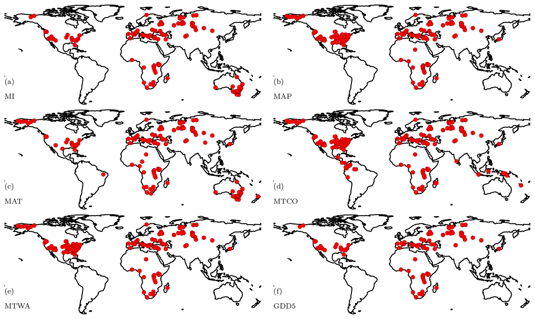
Figure 1 The distribution of the site-based reconstructions of climatic variables at the Last Glacial Maximum. The individual plots show sites providing reconstructions of (a) moisture index (MI), (b) mean annual precipitation (MAP), (c) mean annual temperature (MAT), (d) mean temperature of the coldest month (MTCO), (e) mean temperature of the warmest month (MTWA), and (f)  growing degree days above a baseline of 5 ^∘C (GDD5). The original reconstructions are from Bartlein et al. (2011) and Prentice et al. (2017).

The spatial coverage of the final data set is uneven (Fig. 1). There are many more data points in Europe and North America than elsewhere. South America has the fewest (14 sites). The number of variables available at each site varies; although most sites (279) have reconstructions of at least three variables, some sites have reconstructions of only one variable (60). Nevertheless, in regions where there is adequate coverage, the reconstructed anomaly patterns are coherent, plausible, and consistent among variables.

For this application, we derived absolute LGM climate reconstructions by adding the reconstructed climate anomalies at each site to the modern climate values from the Climate Research Unit (CRU) historical climatology data set (CRU CL v2.0 data set, New et al., 2002), which provides climatological averages of monthly temperature, precipitation, and cloud cover fraction for the period 1961–1990 CE. Most of the climate variables (MTCO, MTWA, MAT, and MAP) can be calculated directly from the CRU CL v2.0 data set. GDD5 was calculated from pseudo-daily data derived from a linear interpolation of the monthly temperatures. MI was calculated from the CRU climate variables using the radiation calculations in the SPLASH model (Davis et al., 2017). For numerical efficiency, we non-dimensionalized all of the absolute climate reconstructions (and their standard errors) before applying the variational techniques (for details, see Cleator et al., 2020a).

Table 1 Details of the models from the third phase of the Palaeoclimate Modelling Intercomparison Project (PMIP3) that were used for the Last Glacial Maximum (LGM) simulations used to create the prior. Coupled ocean–atmosphere models are indicated as OA; the OAC models have a fully interactive carbon cycle. The resolution in the atmospheric, oceanic, and sea ice components of the models is given in terms of numbers of grid cells in latitude and longitude.

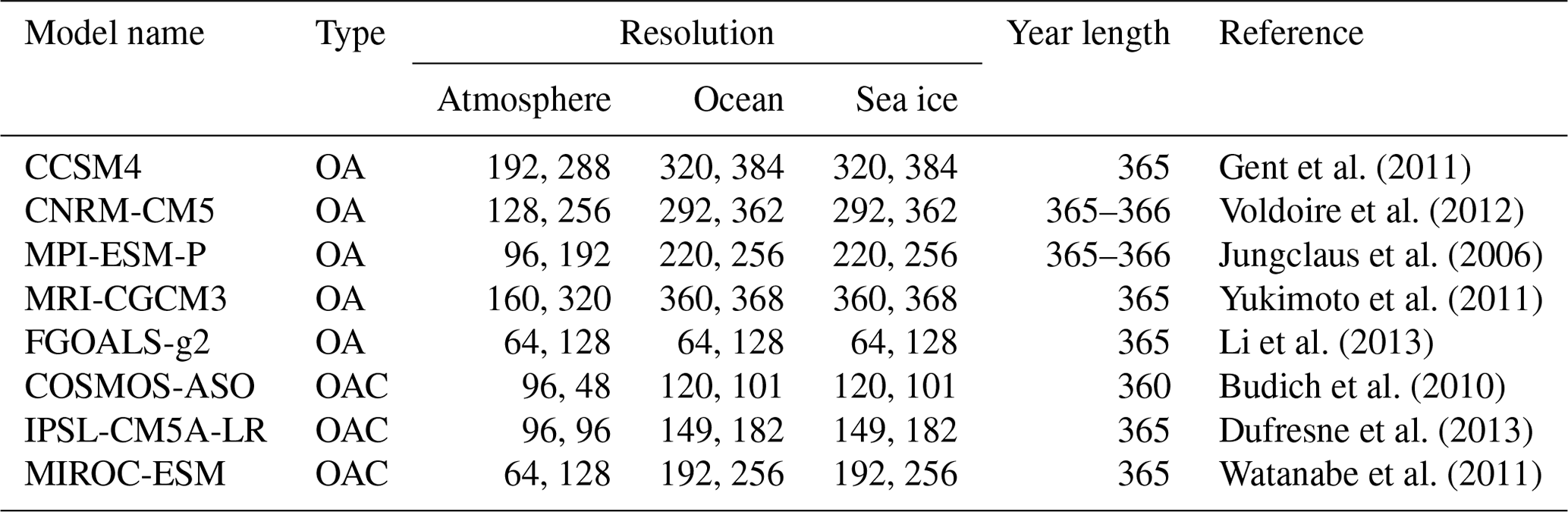
2.2 Climate model simulations

Eight LGM climate simulations (Table 1) from the third phase of the Palaeoclimate Modelling Intercomparison Project (PMIP3; Braconnot et al., 2012) were used to create a prior. The PMIP LGM simulations were forced by known changes in incoming solar radiation, changes in land–sea geography and the extent and location of ice sheets, and a reduction in [CO₂] to 185  ppm (see Braconnot et al., 2012, for details of the modelling protocol). We used the last 100 years of each LGM simulation. We interpolated monthly precipitation, monthly temperature, and monthly fraction of sunshine hours from each LGM simulation and its pre-industrial (PI) control to a common $\mathrm{2}{}^{\circ }\times \mathrm{2}{}^{\circ }$ grid. Simulated climate anomalies (LGM minus PI) for each grid cell were then added to modern climate values calculated from the CRU CL v2.0 data set (New et al., 2002), as described for the pollen-based reconstructions, to derive absolute climate values. We calculated the multi-model mean and variance (Fig. 2) across the models for each of the climate variables to produce the gridded map used as the prior.

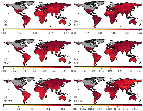
Figure 2 Uncertainties associated with the climate prior. The climate is derived from a multi-model mean of the ensemble of models from the Palaeoclimate Modelling Intercomparison Project (PMIP) and is shown in Fig. S1 in the Supplement. The uncertainties shown here are the standard deviation of the multi-model ensemble values. The individual plots show the variance for the simulated (a) moisture index (MI), (b) mean annual precipitation (MAP), (c) mean annual temperature (MAT), (d) mean temperature of the coldest month (MTCO), (e) mean temperature of the warmest month (MTWA), and (f) growing degree days above a baseline of 5 ^∘C (GDD5).

2.3 Water-use efficiency calculations

We applied the general approach developed by Prentice et al. (2017) to correct pollen-based statistical reconstructions to account for [CO₂] effects. The approach as implemented here is based on equations (Appendix A) that link moisture index (MI) to transpiration and the ratio of internal leaf to ambient [CO₂]. The correction is based on the principle that the rate of water loss per unit carbon gain is inversely related to effective moisture availability as sensed by plants. The method involves solving a nonlinear equation that relates rate of water loss per unit carbon gain to MI, temperature, and CO₂ concentration. The equation is derived from a theory that predicts the response of the ratio of internal leaf to ambient [CO₂] to vapour pressure deficit and temperature (Prentice et al., 2014; Wang et al., 2014).

2.4 Application of variational techniques

Variational data assimilation techniques provide a way of combining observations and model outputs to produce climate reconstructions that are not exclusively constrained to one source of information or the other (Nichols, 2010). We use the 3-D variational method, described in Cleator et al. (2020a), to find the maximum a posteriori estimate (or analytical reconstruction) of the palaeoclimate given the site-based reconstructions and the model-based prior. The method constructs a cost function, which describes how well a particular climate matches both the site-based reconstructions and the prior, by assuming the reconstructions and prior have a Gaussian distribution. To avoid sharp changes in time and/or space in the analytical reconstructions, the method assumes that the prior temporal and spatial covariance correlations are derived from a modified Bessel function, in order to create a climate anomaly field that is smooth both from month to month and from grid cell to grid cell. The degree of correlation is controlled through two length scales: a spatial length scale that determines how correlated the covariance in the prior is between different geographical areas and a temporal length scale that determines how correlated it is through the seasonal cycle. The site-based reconstructions are assumed to have negligible correlations at these scales of space and time. The maximum a posteriori estimate is found by using the limited memory Broyden–Fletcher–Goldfarb–Shanno method (Liu and Nocedal, 1989) to determine the climate that minimizes the cost function. A 1st-order estimate of the analysis uncertainty covariance is also computed.

An observation operator based on calculations of the direct impact of [CO₂] on water-use efficiency (Sect. 2.3) is used in making the analytical reconstructions. The prior is constructed as the average of eight LGM climate simulations (Sect. 2.2). We use an ensemble of different model responses to the same forcing to provide a series of physically consistent possible states, which can be viewed as perturbed responses and provide the variance around the climatology provided by the ensemble average. The prior uncertainty correlations are based on a temporal length scale (Lt) of 1 month and a spatial length scale (Ls) of 400 km. Cleator et al. (2020a) have shown that a temporal length scale of 1 month provides an adequately smooth solution for the seasonal cycle, both using single sites and over multiple grid cells, as shown by the sensitivity of the resolution matrix (Menke, 2012; Delahaies et al., 2017) to changes in the temporal length scale. Consideration of the spatial spread of variance in the analytical reconstruction shows that a spatial length scale of 400 km also provides a reasonable reflection of the large-scale coherence of regional climate change.

Figure 3 Uncertainties in the analytical reconstructions. These uncertainties represent a combination of the uncertainty in the site-based reconstructions and the grid-based variance in the prior and the global variance from the prior.

We generated composite variances on the analytical reconstructions (Fig. 3) by combining the covariances from the site-based reconstructions and the prior. There are regions where all of the models systematically differ from the site-based reconstructions (Harrison et al., 2015), but, nevertheless, the inter-model variability is low, which would lead to a very small contribution to the composite uncertainties from the prior. We therefore calculated the uncertainty of the prior from an equal combination of the global uncertainty, the average variance between each grid cell, and local uncertainty (the variance between the different models). The reliability of the analytical reconstructions was assessed by comparing these composite covariances with the uncertainties in the prior. We masked out cells where the inclusion of site-based reconstructions does not produce an improvement of > 5 % from the prior. Since this assessment is based on a change in the variance, rather than absolute values, this masking removes regions where there are no pollen-based reconstructions or the pollen-based reconstructions have very large uncertainties.

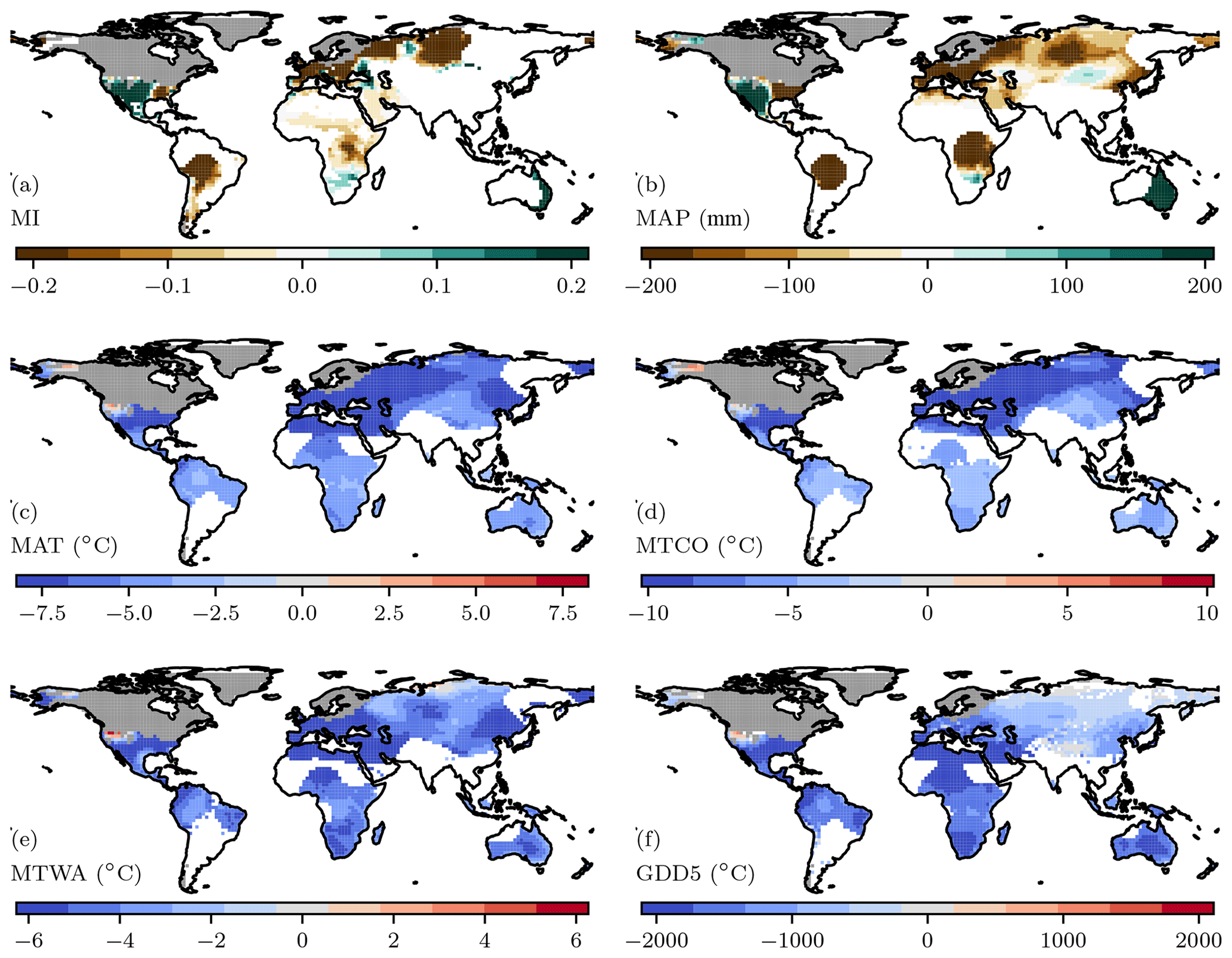
Figure 4 Analytically reconstructed climate, where areas for which the site-based data provide no constraint on the prior have been masked out. The individual plots show reconstructed (a) moisture index (MI), (b) mean annual precipitation (MAP), (c) mean annual temperature (MAT), (d) mean temperature of the coldest month (MTCO), (e) mean temperature of the warmest month (MTWA), and (f)  growing degree days above a baseline of 5 ^∘C (GDD5). The anomalies are expressed relative to the long-term average (1960–1990) values from the Climate Research Unit (CRU) historical climatology data set (CRU CL v2.0 data set, New et al., 2002).

3 Results

The analytical reconstructions (Fig. 4) show an average year-round cooling of −7.9 ^∘C in the northern extratropics. The cooling is larger in winter (−10.2 ^∘C) than in summer (−4.7 ^∘C). A limited number of grid cells in central Eurasia show higher MAT. Temperature changes are more muted in the tropics, with an average change in MAT of −4.7 ^∘C. The cooling is somewhat lower in summer than winter (−3.7 ^∘C compared to −4.1 ^∘C). Reconstructed temperature changes were slightly smaller in the southern extratropics, with average changes in MAT of −3.0 ^∘C, largely driven by cooling in winter.

Changes in moisture-related variables (MAP, MI) across the Northern Hemisphere are geographically more heterogeneous than temperature changes. Reconstructed MAP is greater than present in western North America (204 mm) but less than present in eastern North America (−276 mm). Most of Europe is reconstructed as drier than present (−386 mm), the same for eastern Eurasia (−118 mm) and the Far East (−88 mm). The patterns in MI are not identical to those in MAP, because of the influence of temperature on MI, but regional changes are generally similar to those shown by MAP. Most of the tropics are shown as drier than present while the Southern Hemisphere extratropics are wetter than present, in terms of both MAP and MI.

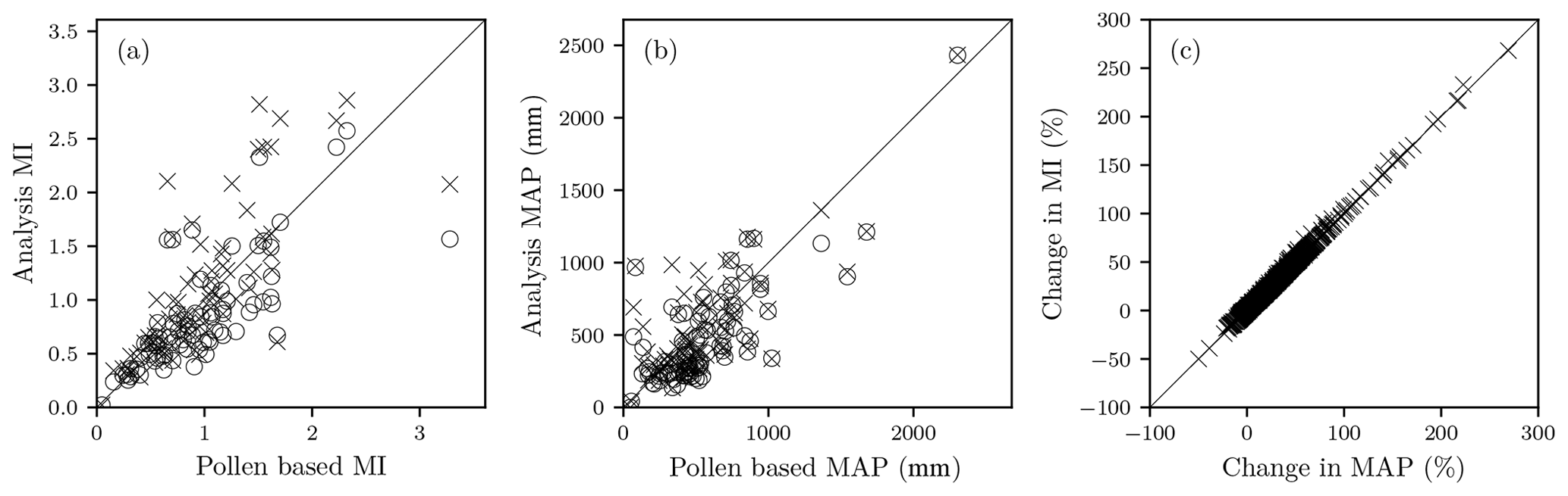
Figure 5 Impact of [CO₂] on reconstructions of moisture-related variables. The individual plots show (a) the change in moisture index (MI) and (b) the change in mean annual precipitation (MAP) compared to the original pollen-based reconstructions for the LGM before (circles) and after (crosses) the physiological impacts of [CO₂] on water-use efficiency are taken into account. The third plot (c) shows the relative difference between MI and MAP as a result of [CO₂], shown as the percentage difference between the no-[CO₂] and [CO₂] calculations.

The reconstructed temperature patterns are not fundamentally different from those shown by Bartlein et al. (2011), but the analytical data set provides information for a much larger area (755 % increase), thanks to the imposition of consistency among different climate variables, and of smooth variations both in space and through the seasonal cycle, by the method. There are systematic differences, however, between the analytical reconstructions and the pollen-based reconstructions in terms of moisture-related variables (MAP, MI) because the analytical reconstructions take account of the direct influence of [CO₂] on plant growth. The physiological impact of [CO₂] leads to analytical reconstructions indicating wetter-than-present conditions in many regions (Fig. 5a, b); for example in southern Africa, several of the original pollen-based reconstructions show no change in MAP or MI compared to present, but the analytical reconstruction shows wetter conditions than present. In some regions, incorporating the impact of [CO₂] reverses the sign of the reconstructed changes. Part of northern Eurasia is reconstructed as being wetter than present, despite pollen-based reconstructions indicating conditions drier than present (in terms of both MAP and MI), as shown by Fig. S3. The relative changes in MAP and MI are similar across all sites (Fig. 5c), implying that the analytically reconstructed changes are driven by changes in precipitation rather than temperature.

4 Discussion

Variational data assimilation techniques provide a way of combining observations and model outputs, taking account of the uncertainties in both, to produce a best-estimate analytical reconstruction of LGM climate. These reconstructions extend the information available from site-based reconstructions both spatially and through the seasonal cycle. Our new analytical data set characterizes the seasonal cycle across a much larger region of the globe than the data set that is currently being used for benchmarking of palaeoclimate model simulations. We therefore suggest that this data set (Cleator et al., 2020b) should be used for evaluating the CMIP6–PMIP4 LGM simulations.

Some areas are still poorly covered by quantitative pollen-based reconstructions of LGM climate, most notably South America. More pollen-based climate reconstructions would provide one solution to this problem – and there are many pollen records that could be used for this purpose (Flantua et al., 2015; Herbert and Harrison, 2016; and Harrison et al., 2016). There are also quantitative reconstructions of climate available from individual sites (e.g. Lebamba et al., 2012; Wang et al., 2014; Loomis et al., 2017; and Camuera et al., 2019) that should be incorporated into future data syntheses. It would also be possible to incorporate other sources of quantitative information, such as chironomid-based reconstructions (e.g. Chang et al., 2015), within the variational data assimilation framework.

One of the benefits of the analytical framework applied here is that it allows the influence of changes in [CO₂] on the moisture reconstructions to be taken into account. Low [CO₂] must have reduced plant water-use efficiency, because at low [CO₂] plants need to keep stomata open for longer in order to capture sufficient CO₂. Statistical reconstruction methods that use modern relationships between pollen assemblages and climate under modern conditions (i.e. modern analogues, transfer functions, and response surfaces; see Bartlein et al., 2011) cannot account for such effects. Climate reconstruction methods based on the inversion of process-based ecosystem models can do so (see e.g. Guiot et al., 2000; Wu et al., 2007, 2009; and Izumi and Bartlein, 2016) but are critically dependent on the reliability of the vegetation model used. Most of the palaeoclimate reconstructions have been made by inverting some version of the BIOME model (Kaplan et al., 2003), which makes use of bioclimatic thresholds to separate different plant functional types (PFTs). As a result, reconstructions made by inversion show “jumps” linked to shifts between vegetation types dominated by different PFTs, whereas, as has been shown recently (Wang et al., 2017), differences in water-use efficiency of different PFTs can be almost entirely accounted for by a single equation, as proposed here. Sensitivity analyses show that the numerical value of the corrected moisture variables (MI, MAP) is dependent on the reconstructed values of these variables but is insensitive to uncertainties in the temperature and moisture inputs (Prentice et al., 2017). The strength of the correction is primarily sensitive to [CO₂], but the LGM [CO₂] value is well constrained from ice-core records. The response of plants to changes in [CO₂] is nonlinear (Harrison and Bartlein, 2012), and the effect of the change between recent and pre-industrial or mid-Holocene conditions is less than that between pre-industrial and glacial conditions. Nevertheless, it would be worth taking the [CO₂] effect on water-use efficiency into account in making reconstructions of interglacial time periods as well.

The influence of individual pollen-based reconstructions on the analytical reconstruction of seasonal variability, or the geographic area influenced by an individual site, is crucially dependent on the choice of length scales. We have adopted conservative length scales of 1 month and 400 km, based on sensitivity experiments made for southern Europe (Cleator et al., 2020a). These length scales produce numerically stable results for the LGM, and the paucity of data for many regions at the LGM means that using fixed, conservative length scales is likely to be the only practical approach. However, in so far as the spatial length scale is related to atmospheric circulation patterns, there is no reason to suppose that the optimal spatial length scale will be the same from region to region. The density and clustering of pollen-based reconstructions could also have a substantial effect on the optimal spatial length scale. A fixed 1-month temporal length scale is appropriate for climates that have a reasonably smooth and well-defined seasonal cycle, in either temperature or precipitation. However, in climates where the seasonal cycle is less well defined, for example in the wet tropics, or in situations where there is considerable variability on sub-monthly timescales, other choices might be more appropriate. For time periods such as the mid-Holocene, which have an order of magnitude more site-based data, it could be useful to explore the possibilities of variable length scales.

We have used a 5 % reduction in the analytical uncertainty compared to prior uncertainty to identify regions where the incorporation of site-based data has a negligible effect on the prior as a way of masking out regions for which the observations have effectively no impact on the analytical reconstructions. The choice of a 5 % cut-off is arbitrary, but little would be gained by imposing a more stringent cut-off at the LGM given that many regions are represented by few observations. A more stringent cut-off could be applied for other time intervals with more data. We avoid the use of a criterion based on the analytical reconstruction showing any improvement on the prior because this could be affected by numerical noise in the computation. Alternative criteria for the choice of cut-off could be based on whether the analytical reconstruction had a reduced uncertainty compared to the pollen-based reconstructions or could be derived by a consideration of the condition number used to select appropriate length scales.

There have been a few previous attempts to use data assimilation techniques to generate spatially continuous palaeoclimate reconstructions. Annan and Hargreaves (2013) used a similar multi-model ensemble as the prior and the pollen-based reconstructions from Bartlein et al. (2011) to reconstruct MAT at the LGM. However, they made no attempt to reconstruct other seasonal variables, either independently or through exploiting features of the simulations (as we have done here) to generate seasonal reconstructions. Particle filter approaches (e.g. Goosse et al., 2006; Dubinkina et al., 2011) produce dynamic estimates of palaeoclimate, but particle filters cannot produce estimates of climate outside the realm of the model simulations. Our 3-D variational data assimilation approach has the great merit of being able to produce seasonally coherent reconstructions generalized over space, while at the same time being capable of producing reconstructions that are outside those captured by the climate model, because they are not constrained by a specific source (Nichols, 2010). This property is of particular importance if the resulting data set is to be used for climate model evaluation, as we propose.

Appendix A

We define e as the water lost by transpiration (E) per unit carbon gained by photosynthesis (A). This term, the inverse of the water-use efficiency, is given by

$$\begin{array}{}\text{(A1)}& e=E/A=\mathrm{1.6}D/\left(\right(\mathrm{1}-\mathit{\chi }\left)c_{\mathrm{a}}\right),\end{array}$$

where D is the leaf-to-air vapour pressure deficit (Pa), c_a is the ambient CO₂ partial pressure (Pa), and χ is the ratio of internal leaf CO₂ partial pressure (c_i) to c_a. An optimality-based model (Prentice et al., 2014), which accurately reproduces global patterns of χ and its environmental dependencies inferred from leaf δ¹³C measurements (Wang et al., 2017), predicts that

$$\begin{array}{}\text{(A2a)}& \mathit{\chi }=({\mathrm{\Gamma }}^{*}/c_{\mathrm{a}})+(\mathrm{1}-{\mathrm{\Gamma }}^{*}/c_{\mathrm{a}})\mathit{\xi }/(\mathit{\xi }+\surd D),\end{array}$$

and

$$\begin{array}{}\text{(A2b)}& \mathit{\xi }=\surd \left(\mathit{\beta }\right(K+{\mathrm{\Gamma }}^{*})/\mathrm{1.6}{\mathit{\eta }}^{*}),\end{array}$$

where Γ^* is the photorespiratory compensation point of C₃ photosynthesis (Pa), β is a constant (estimated as 240 by Wang et al., 2017), K is the effective Michaelis–Menten coefficient of Rubisco (Pa), and η^* is the ratio of the viscosity of water (Pa s) at ambient temperature to its value at 25 ^∘C. Here K depends on the Michaelis–Menten coefficients of Rubisco for carboxylation (K_C) and oxygenation (K_O), and on the partial pressure of oxygen O (Farquhar et al., 1980); it is calculated by the following:

$$\begin{array}{}\text{(A3)}& K=K_{\mathrm{C}}(\mathrm{1}+\mathrm{O}/K_{\mathrm{O}}).\end{array}$$

Standard values and temperature dependencies of K_C, K_O, Γ^*, and η^* are assigned as in Wang et al. (2017).

The moisture index MI is expressed as

$$\begin{array}{}\text{(A4)}& \mathrm{MI}=P/E_q,E_q={\sum }_n(R_n/\mathit{\lambda })s/(s+\mathit{\gamma }),\end{array}$$

where P is annual precipitation, R_n is net radiation for month n, λ is the latent heat of vaporization of water, s is the derivative of the saturated vapour pressure of water with respect to temperature (obtained from a standard empirical formula also used by Wang et al., 2017), and γ is the psychrometer constant. We assume that values of MI reconstructed from fossil pollen assemblages, using contemporary pollen and climate data either in a statistical calibration method or in a modern-analogue search, need to be corrected in such a way as to preserve the contemporary relationship between MI and e, while taking into account the change in e that is caused by varying c_a and temperature away from contemporary values. The sequence of calculations is as follows. (1) Estimate e and its derivative with respect to temperature ($\partial e/\partial T$) for the contemporary c_a and climate, using Eqs. (A1)–(A3) above. (2) Use e and $\partial e/\partial$ T to calculate $\partial D/\partial T$ given the palaeo-c_a (measured in ice-core data) and temperature (reconstructed from pollen data), via a series of analytical equations that relate $\partial e/\partial T$ to $\partial D/\partial T$ and hence to s. (3) Use the new $\partial D/\partial$ T and relative humidity (from the PMIP3 average) to derive a new value of s. (4) Recalculate MI using a palaeo-estimate of R_n (modelled as in Davis et al., 2017) and the new value of s.