OPTiMAL: a new machine learning approach for GDGT-based palaeothermometry

In the modern oceans, the relative abundances of glycerol dialkyl glycerol tetraether (GDGT) compounds produced by marine archaeal communities show a significant dependence on the local sea surface temperature at the site of deposition. When preserved in ancient marine sediments, the measured abundances of these fossil lipid biomarkers thus have the potential to provide a geological record of long-term variability in planetary surface temperatures. Several empirical calibrations have been made between observed GDGT relative abundances in late Holocene core-top sediments and modern upper ocean temperatures. These calibrations form the basis of the widely used TEX₈₆ palaeothermometer. There are, however, two outstanding problems with this approach: first the appropriate assignment of uncertainty to estimates of ancient sea surface temperatures based on the relationship of the ancient GDGT assemblage to the modern calibration dataset, and second, the problem of making temperature estimates beyond the range of the modern empirical calibrations (> 30 ^∘C). Here we apply modern machine learning tools, including Gaussian process emulators and forward modelling, to develop a new mathematical approach we call OPTiMAL (Optimised Palaeothermometry from Tetraethers via MAchine Learning) to improve temperature estimation and the representation of uncertainty based on the relationship between ancient GDGT assemblage data and the structure of the modern calibration dataset. We reduce the root mean square uncertainty on temperature predictions (validated using the modern dataset) from ∼ ±6 ^∘C using TEX₈₆-based estimators to ±3.6 ^∘C using Gaussian process estimators for temperatures below 30 ^∘C. We also provide a new quantitative measure of the distance between an ancient GDGT assemblage and the nearest neighbour within the modern calibration dataset, as a test for significant non-analogue behaviour.

1 Introduction

Glycerol dibyphytanyl glycerol tetraethers (GDGTs) are membrane lipids consisting of isoprenoid carbon skeletons ether-bound to glycerol (Schouten et al., 2013). In marine systems they are primarily produced by ammonia oxidising marine Thaumarchaeota (Schouten et al., 2013). In modern marine core-top sediments, the relative abundance of GDGT compounds with more ring structures increases with the mean annual sea surface temperature (SST) of the overlying waters (Schouten et al., 2002). This trend is most likely driven by the need for increased cell membrane stability and rigidity at higher temperatures (Sinninghe Damsté et al., 2002). On this basis, the TEX₈₆ (tetraether index of tetraethers containing 86 carbon atoms) ratio was derived to provide an index to represent the extent of cyclisation (Eq. 1; where GDGT-x represents the fractional abundance of GDGTs determined by liquid chromatography mass spectrometry (LC-MS) peak area, and cren^′ is the peak area of the isomer of crenarchaeol, cren) (Schouten et al., 2002; Kim et al., 2010) and was shown to be positively correlated with mean annual SSTs:

$$\begin{array}{}\text{(1)}& \begin{array}{rl}{\text{TEX}}_{\mathrm{86}}& =\left(\text{GDGT-2}+\text{GDGT-3}+{\text{cren}}^{\prime }\right)/\\ & \left(\text{GDGT-1}+\text{GDGT-2}+\text{GDGT-3}+{\text{cren}}^{\prime }\right).\end{array}\end{array}$$

Early applications of TEX₈₆ to reconstruct ancient SSTs were promising, especially in providing temperature estimates in environments where standard carbonate-based proxies are hampered by poor preservation (Schouten et al., 2003; Herfort et al., 2006; Schouten et al., 2007; Huguet et al., 2006; Sluijs et al., 2006; Brinkhuis et al., 2006; Pearson et al., 2007; Slujis et al., 2009). The TEX₈₆ approach also extended beyond the range of the widely used alkenone-based $U_{\mathrm{37}}^{k^{\prime }}$ thermometer, in both temperature space, where $U_{\mathrm{37}}^{k^{\prime }}$ saturates at ∼ 28 ^∘C (Brassell, 2014), and back into the early Cenozoic (Bijl et al., 2009; Hollis et al., 2009; Bijl et al., 2013; Inglis et al., 2015) and Mesozoic (Schouten et al., 2002; Jenkyns et al., 2012; O'Brien et al., 2017) where haptophyte-derived alkenones are typically absent from marine sediments (Brassell, 2014). Initially, TEX₈₆ was converted to SSTs using the core-top calibration (Schouten et al., 2002) (Eq. 2):

$$\begin{array}{}\text{(2)}& {\text{TEX}}_{\mathrm{86}}=\mathrm{0.015}\times \text{SST}+\mathrm{0.28}.\end{array}$$

However, as the number and range of applications of TEX₈₆ palaeothermometry grew, concerns arose about proxy behaviour at both the high (Liu et al., 2009) and low (Kim et al., 2008) temperature ends of the modern calibration. In response to these observations, a new expanded modern core-top dataset (Kim et al., 2010) was used to generate two new indices – TEX${}_{\mathrm{86}}^{\text{L}}$ (Eq. 3), an exponential function that does not include the crenarchaeol regio-isomer and was recommended for use across the entire temperature range of the new core-top data (−3 to 30 ^∘C, particularly when SSTs are lower than 15 ^∘C), and ${\text{TEX}}_{\mathrm{86}}^{\text{H}}$ (Eq. 4), also exponential, and recommended for use when SSTs exceeded 15 ^∘C (Kim et al., 2010). ${\text{TEX}}_{\mathrm{86}}^{\text{L}}$ also excludes GDGT abundance data from the high-temperature regimes of the Red Sea, which are somewhat anomalous and likely related to salinity effects on community composition in this region (Trommer et al., 2009; Kim et al., 2010).

$$\begin{array}{}\text{(3)}& {\displaystyle }{\text{TEX}}_{\mathrm{86}}^{\text{L}}=\log \left({\displaystyle \frac{\left[\text{GDGT-2}\right]}{\left[\text{GDGT-1}\right]+\left[\text{GDGT-2}\right]+\left[\text{GDGT-3}\right]}}\right)\text{(4)}& {\displaystyle }\begin{array}{rl}& {\text{TEX}}_{\mathrm{86}}^{\text{H}}=\\ & \log \left({\displaystyle \frac{\left[\text{GDGT-2}\right]+\left[\text{GDGT-3}\right]+\left[{\text{cren}}^{\prime }\right]}{\left[\text{GDGT-1}\right]+\left[\text{GDGT-2}\right]+\left[\text{GDGT-3}\right]+\left[{\text{cren}}^{\prime }\right]}}\right)\end{array}\end{array}$$

Both ${\text{TEX}}_{\mathrm{86}}^{\text{H}}$ and ${\text{TEX}}_{\mathrm{86}}^{\text{L}}$ were widely used and tested across a range of temperatures and palaeoenvironments, including comparisons against other palaeotemperature proxy systems (Hollis et al., 2012; Lunt et al., 2012; Bijl et al., 2013; Dunkley Jones et al., 2013; Zhang et al., 2014; Seki et al., 2014; Douglas et al., 2014; Linnert et al., 2014; Hertzberg et al., 2016). In certain environments ${\text{TEX}}_{\mathrm{86}}^{\text{L}}$ was subject to significant variability in derived temperatures that were not apparent in ${\text{TEX}}_{\mathrm{86}}^{\text{H}}$ (Taylor et al., 2013). This was mostly due to changing GDGT-2-to-GDGT-3 ratios, which strongly influence ${\text{TEX}}_{\mathrm{86}}^{\text{L}}$, and may be related to local non-thermal environmental conditions at the site of GDGT production, and deep-water lipid production (Taylor et al., 2013). As a result, ${\text{TEX}}_{\mathrm{86}}^{\text{L}}$ is no longer regarded as an appropriate tool for palaeotemperature reconstructions, except in limited polar conditions (Kim et al., 2010; Tierney, 2012).

Ongoing work to strengthen GDGT-based palaeothermometry is focused on three key issues. The first is a concern about undetected non-analogue palaeo-GDGT assemblages, for which the modern calibration dataset is inadequate to provide a robust temperature estimation. Although various screening protocols, with independent indices and thresholds, have been proposed to test for an excessive influence of terrestrial lipids (branched and isoprenoid tetraether, BIT index; Hopmans et al., 2004), within sediment methanogenesis (methane index, MI; Zhang et al., 2011) and non-thermal effects such as nutrient levels and archaeal community structure to impact the weighted average of cyclopentane moieties (ring index, RI; Zhang et al., 2016), these do not provide a fundamental measure of the proximity between GDGT abundance distributions in the modern calibration data set and ancient GDGT abundance distributions recorded in sediment samples. The fundamental question remains – are measured ancient assemblages of GDGT compounds anything like the modern assemblages, from which palaeotemperatures are being estimated? Understanding this question cannot easily be addressed with the use of indices – TEX₈₆ itself, or BIT and MI – that collapse the dimensionality of GDGT abundance relationships onto a single axis of variation.

Second, from the earliest applications of the TEX₈₆ proxy to deep-time warm climate states (Schouten et al., 2003) it was recognised that reconstructed temperatures beyond the range of the modern calibration (> 30 ^∘C) were highly sensitive to model choice within the modern calibration range. Thus, Schouten et al. (2003) restricted their calibration data for deep-time temperature estimates to core-top data in the modern era with mean annual SSTs over 20 ^∘C. However, this problem of model choice, and its impact on temperature estimation beyond the modern calibration range, persists (Hollis et al., 2019), with current arguments focused on whether there is an exponential (e.g. Cramwinckel et al., 2018) or linear (Tierney and Tingley, 2015) dependency of TEX₈₆ on SSTs, and the effect of these models on temperature estimates over 30 ^∘C.

Culture and mesocosm studies are sometimes cited in support of extrapolations beyond the modern calibration range when reconstructing ancient SSTs (Kim et al., 2010, Hollis et al., 2019). While there is a basic underlying trend for more rings within GDGT structures at higher temperatures (Zhang et al., 2016; Qin et al., 2015), the lack of a uniform response to archaeal GDGT production in response to increasing growth temperatures (e.g. Elling et al., 2015; Qin et al., 2015) suggests that this does not easily translate into a simple linear model at the community scale (i.e. the core-top calibration dataset). In natural systems, it is likely that aggregated GDGT abundance variations in response to growth temperatures result from changing compositions of archaeal populations as well as the physiological response of individual strains to growth temperature (Elling et al., 2015; Polik et al., 2018). For deep-time applications it is even more difficult, where there is no independent constraint on the archaeal strains dominating production or their evolution through time (Elling et al., 2015). What is notable, however, is that the RI – calculated using all commonly measured GDGTs (Zhang et al., 2016) – has a more robust relationship with culture temperature between archaeal strains than TEX₈₆, indicating a potential loss of information within the TEX₈₆ index (Elling et al., 2015).

Finally, under some conditions, the original TEX₈₆ proxy had a relatively poor representation of the true uncertainty associated with palaeotemperature estimates, as it included no assessment of non-analogue behaviour relative to the modern core-top data. Instead, uncertainty was typically based on the residuals on the modern calibration, with no reference to the relationship between GDGT distributions of an ancient sample and the modern calibration data. An improved Bayesian uncertainty model “BAYSPAR” is now in widespread use for SST estimation, which models TEX₈₆ to SST regression parameters, and associated uncertainty, as spatially varying functions (Tierney and Tingley, 2015). The Bayesian approach, as with all approaches based on the TEX₈₆ index, however, still does not include an uncertainty that reflects how well modelled ancient GDGT assemblages are by the modern calibration – i.e. the degree to which they are non-analogue – as it still functions on one-dimensional TEX₈₆ index values.

All empirical calibrations of GDGT-based proxies assume that mean annual SST is the master variable on GDGT assemblages both today and in the past. Mean annual SST, however, is strongly correlated with many other environmental variables (e.g. seasonality, pH, mixed layer depth and productivity). In the modern calibration dataset, mean annual SST shows the strongest correlation with TEX₈₆ index (Schouten et al., 2002), but this does not preclude an important (but undetectable) influence of these other environmental variables. The use of empirical GDGT calibrations to infer ancient sea surface temperatures thus implicitly assumes that the relationships between mean annual SST and all other GDGT-influencing variables are invariant through time. This assumption is inescapable until, and unless, a more complete biological mechanistic model of GDGT production emerges.

Here, we return to the primary modern core-top GDGT assemblage data (Tierney and Tingley, 2015), and systematically explore the relationships between the modern GDGT distributions and surface ocean temperatures using powerful mathematical tools. These tools can investigate correlations without prior assumptions on the best form of relationship or a priori selection of GDGT compounds to be used. This analysis is then extended through the exploration of the relationships between the modern core-top GDGT distributions and two compilations of ancient GDGT datasets, one from the Eocene (Inglis et al., 2015) and one from the Cretaceous (O'Brien et al., 2017). We explore simple metrics to answer the fundamental question – are modern core-top GDGT distributions good analogues for ancient distributions? We propose the first robust methodology to answer this question, and so screen for significantly non-analogue palaeo-assemblages. From this, we go on to derive a new machine learning approach “OPTiMAL” (Optimised Palaeothermometry from Tetraethers via MAchine Learning) for reconstructing SSTs from GDGT datasets, which outperforms previous GDGT palaeothermometers and includes robust error estimates that, for the first time, accounts for model uncertainty.

2 Models for GDGT-based temperature reconstruction

Our new analyses use the modern core-top data compilation, and satellite-derived estimates of SSTs, of Tierney and Tingley (2015) as well as compilations of Eocene (Inglis et al., 2015) and Cretaceous (O'Brien et al., 2017) GDGT assemblages. Within these fossil assemblages, only data points with full characterisation of individual GDGT relative abundances were used. We also note that, in the first instance, all available fossil assemblage data were included, although later comparisons between BAYSPAR and our new temperature predictor excludes fossil data that was regarded as unreliable based on standard pre-screening indices, as noted within the original compilations (Inglis et al., 2015; O'Brien et al., 2017). All data used in this study are tabulated in the Supplement.

In order to enable meaningful comparison between new and existing temperature predictors, we use the following consistent procedure for evaluating all predictors throughout this paper. We divide the modern core-top dataset of 854 data points into 85 validation data points (chosen randomly) and 769 calibration points (as we require fractional abundances for all 6 commonly measured GDGTs, we excluded those data points for which these values were not reported). We calibrate the predictor on the calibration points and then judge its performance on the validation points using the root mean square error:

$$\begin{array}{}\text{(5)}& \mathit{\delta }T=\sqrt{{\displaystyle \frac{\mathrm{1}}{N_{\mathrm{v}}-\mathrm{1}}}{\sum }_{k=\mathrm{1}}^{N_{\mathrm{v}}}{\left(\widehat{T}\left(x_k\right)-T\left(x_k\right)\right)}^{\mathrm{2}}},\end{array}$$

where the sum is taken over each of N_v=85 validation points, T is the known measured temperature (which we refer to as the true temperature) and $\widehat{T}$ is the predicted temperature. For conciseness, we refer to δT as the predictor standard error. It is useful to compare the accuracy of the predictor to the standard deviation of all temperatures in the dataset σT, which corresponds to using the mean temperature as the predictor in Eq. (1); for the modern dataset, σT=10.0 ^∘C. The coefficient of determination, R², provides a measure of the fraction of the fluctuation in the temperature explained by the predictor. To facilitate performance comparisons between different methods of predicting temperature, we use the same subset of validation points for all analyses. To avoid sensitivity to the choice of validation points, we repeat the calibration–validation procedure for 10 random choices from the validation dataset.

2.1 Nearest neighbours

We begin with an agnostic approach to using some combination of the proportions of each of the six observables – GDGT-0, GDGT-1, GDGT-2, GDGT-3, crenarchaeol and cren^′, which we will jointly refer to as GDGTs – to predict sea surface temperatures. Whatever functional form the predictor might take, it can only provide accurate temperature predictions if nearby points in the six-dimensional observable space – i.e. the distribution of all of the six commonly reported GDGTs – can be translated to nearby points in temperature space. Conversely, if nearby points in the observable space correspond to vastly different temperatures, then no predictor, regardless of which combination of GDGTs are used, will be able to provide a useful temperature estimate. In other words, the structuring of GDGT distributions within multi-dimensional space must have some correspondence to the temperatures of formation (or rather the mean annual SSTs used for standard calibrations).

We therefore consider the prediction offered by the temperature at the nearest point in the GDGT parameter space. Of course, nearness depends on the choice of the distance metric. For example, it may be that sea surface temperatures are very sensitive to a particular GDGT, so even a small change in that GDGT corresponds to a significant distance, and rather insensitive to another, meaning that even with a large difference in the nominal value of that GDGT the distance is insignificant. In the first instance, we use a very simple Euclidian distance estimate D_x,y where the distance along each GDGT is normalised by the total spread in that GDGT across the entire dataset. This normalisation ensures that a dimensionless distance estimate can be produced even when observables have very different dynamical ranges, or even different units. Thus, the normalised distance D between parameter data points x and y is

$$\begin{array}{}\text{(6)}& D_{x,y}^{\mathrm{2}}\equiv {\sum }_{i=\mathrm{0}}^{\mathrm{5}}{\displaystyle \frac{{\left({\mathrm{GDGT}}_i\left(x\right)-{\mathrm{GDGT}}_i\left(y\right)\right)}^{\mathrm{2}}}{\mathrm{var}\left({\mathrm{GDGT}}_i\right)}}.\end{array}$$

We show the distribution of nearest distances of points in the modern dataset, excluding the sample itself, in Fig. 1.

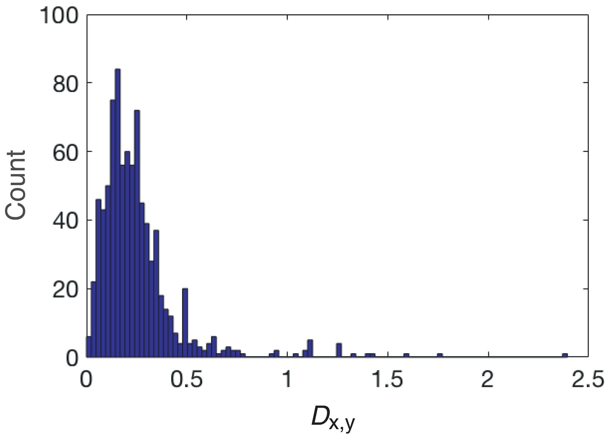
Figure 1 A histogram of the normalised distance to the nearest neighbour in GDGT space (D_x,yt) for all samples in the modern calibration dataset of Tierney and Tingley (2015).

The nearest-sample temperature predictor is ${\widehat{T}}_{\mathrm{nearest}}\left(x\right)=T\left(y\right)$, where y is the nearest point to x over the calibration dataset, i.e. one that minimises D_x,y. Figure 2 shows the scatter in the predicted temperature when using the temperature of the nearest data point to make the prediction. Overall, the failure of the nearest-neighbour predictor to provide accurate temperature estimates even when the normalised distance to the nearest point is small, $D_{x,y}\le \mathrm{0.5}$, casts doubt on the possibility of designing an accurate predictor for temperature based on GDGT observations. This is most likely due to additional environmental controls on GDGT abundance distributions in natural systems, in particular the water depth (Zhang and Liu, 2018), nutrient availability (Hurley et al., 2016; Polik et al., 2018; Park et al., 2018), seasonality, growth rate (Elling et al., 2014; Hurley et al., 2016) and ecosystem composition (Polik et al., 2018), that obscure a predominant relationship to mean annual SSTs.

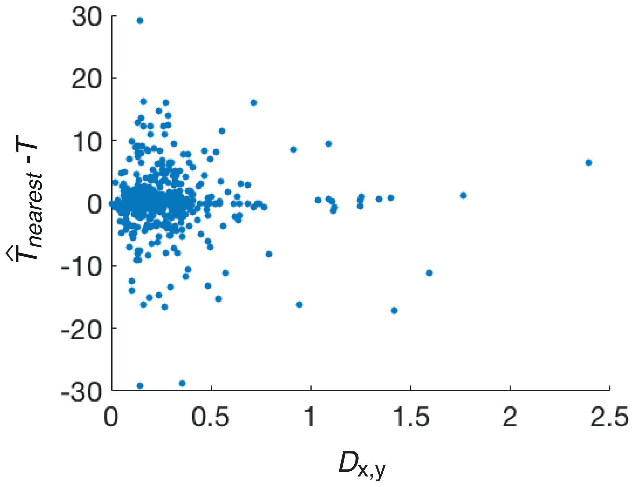
Figure 2 The error of the nearest-neighbour temperature (D_x,y) predictor, for modern core-top data, as a function of the distance to the nearest calibration sample.

On the other hand, the standard error for the nearest-neighbour temperature predictor is δT_nearest=4.5 ^∘C. This is less than half of the standard deviation σT in the temperature values across the modern dataset. Thus, the temperatures corresponding to nearby points in GDGT observable space also cluster in temperature space. Consequently, there is hope that we can make some useful, if imperfect, temperature predictions. The value of δT_nearest will also serve as a useful benchmark in this design: while we may hope to do better by, say, suitably averaging over multiple nearby calibration points rather than adopting the temperature at one nearest point as a predictor, any method that performs worse than the nearest-neighbour predictor is clearly suboptimal.

2.2 TEX₈₆ and Bayesian applications

The TEX₈₆ index reduces the six-dimensional observable GDGT space to a single number. While this has the advantage of convenience for manipulation and the derivation of simple analytic formulae for predictors, as illustrated below, this approach has one critical disadvantage: it wastes significant information embedded in the hard-earned GDGT distribution data. Figure 3 illustrates both the advantage and disadvantage of TEX₈₆. On the one hand, there is a clear correlation between TEX₈₆ and temperature (Fig. 3a), with a correlation coefficient of 0.81 corresponding to an overwhelming statistical significance of 10⁻¹⁹⁸. On the other hand, very similar TEX₈₆ values can correspond to very different temperatures. We can apply the nearest-neighbour temperature prediction approach to the TEX₈₆ value alone rather than the full GDGT parameter space; this predictor yields a large standard error of $\mathit{\delta }{T}_{{\text{nearest TEX}}_{\mathrm{86}}}=\mathrm{8.0}$ ^∘C (bottom panel of Fig. 3). While smaller than σT, this is significantly larger than δT_nearest (Fig. 2), consistent with the loss of information in TEX₈₆. We therefore do not expect other predictors based on TEX₈₆ to perform as well as those based on the full available dataset.

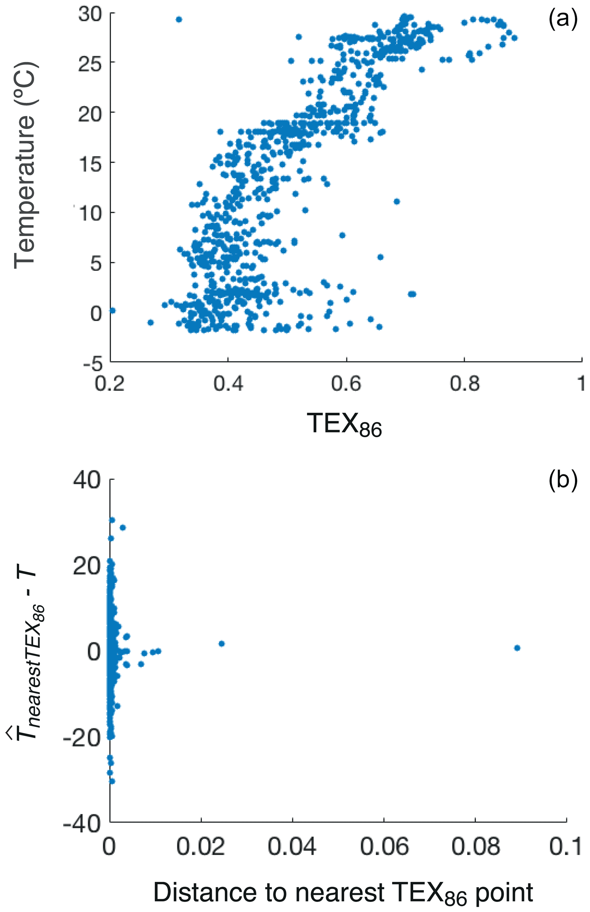
Figure 3 (a) The temperature of the modern dataset as a function of the TEX₈₆ value, showing a clear linear correlation between the two, but also significant scatter. (b) The error of the predictor based on the nearest TEX₈₆ calibration point.

Indeed, this is what we find when we consider predictors of the form ${\widehat{T}}_{\mathrm{1}/\text{TEX}}=a+b/{\text{TEX}}_{\mathrm{86}}$ and ${\widehat{T}}_{\mathrm{TEXH}}=c+d{\log }_{{\text{TEX}}_{\mathrm{86}}}$ (Liu et al., 2009; Kim et al., 2010), i.e. the established relationships between GDGT distributions and SST. We fit the free parameters a, b, c and d by minimising the sum of squares of the residuals over the calibration datasets (least squares regression). We find that $\mathit{\delta }{T}_{\mathrm{1}/\text{TEX}}=\mathrm{6.1}$ ^∘C (note that this is slightly better than using the fixed values of a and b from Kim et al. (2010), which yield $\mathit{\delta }{T}_{\mathrm{1}/\text{TEX}}=\mathrm{6.2}$ ^∘C). We note that the corresponding R² value associated with these TEX₈₆-based predictors is 0.64, which is lower than the R² values in Kim et al. (2010). We attribute this to the fact that we are using a larger dataset based on Tierney and Tingley (2015), including data from the Red Sea (Kim et al., 2010).

Tierney and Tingley (2014) proposed a more sophisticated approach to obtaining the transfer function from TEX₈₆ to temperature, continuing to use simple linear regression, but with the addition of Gaussian processes to model spatial variability in the temperature–TEX₈₆ relationship and working with a forward model which is subsequently inverted to produce temperature predictions. This forward model “BAYSPAR” is capable of generating an infinite number of calibration curves relating TEX₈₆ to sea surface temperatures (Tierney and Tingley, 2014). In order to derive a calibration for a specific dataset, the user edits a range of parameters which vary depending on whether the dataset in question is from the relatively recent past or deep time (Tierney and Tingley, 2014). For deep time applications, the authors propose a modern analogue-type approach, in which they search the modern data for $\mathrm{20}{}^{\circ }\times \mathrm{20}{}^{\circ }$ grid boxes containing “nearby” TEX₈₆ measurements and subsequently apply linear regression models calibrated on the analogous samples for making predictions.

However, along with the simpler TEX₈₆-based models described above, this approach still suffers from the reduction of a six-dimensional dataset to a single number. Therefore, it is not surprising that even the simplest nearest-neighbour predictor (such as the one described above) that makes use of the full six-dimensional dataset outperforms single-dimensional forward modelling approaches. Additionally, uncertainty estimates do not account for the fact that TEX₈₆ is, fundamentally, an empirical proxy, and so its validity outside the range of the modern calibration is not guaranteed. This is a fundamental issue for attempts to reconstruct surface temperatures during greenhouse climate states, when tropical and sub-tropical SSTs were likely hotter than those observed in the modern oceans.

2.3 Machine learning approaches – random forests

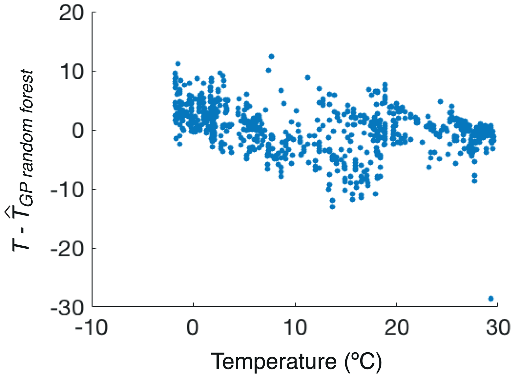
There are a number of options to improve on nearest-neighbour predictions using machine learning techniques such as artificial neural networks and random forests. These flexible, non-parametric models would ideally be based on the underlying processes driving the GDGT response to temperature, but since these processes remain unconstrained at present, we choose to deploy models which can reasonably reflect predictive uncertainty and will be sufficiently adaptable in future (as new information regarding controls on GDGTs emerge). These machine learning approaches are all based on the idea of training a predictor by fitting a set of coefficients in a sufficiently complex multi-layer model in order to minimise residuals on the calibration dataset. As an example of the power of this approach, we train a random forest of decision trees with 100 learning cycles using a least-squares boosting to fit the regression ensemble. Figure 4 shows the prediction accuracy for this random forest implementation. This machine learning predictor yields δT=4.1 ^∘C, outperforming the naive nearest-neighbour predictor by effectively applying a suitable weighted average over multiple near neighbours. This corresponds to a very respectable R²=0.83, meaning that 83 % of the variation in the observed temperature is successfully explained by our GDGT-based model.

Figure 4 The error of a random forest predictor as a function of the true temperature.

2.4 Gaussian process regression

One downside of the random forest predictor is the difficulty of accurately estimating the uncertainty of the prediction (Mentch and Hooker, 2016), although this is possible with, for example, a bootstrapping approach (Coulston et al., 2016). Fortunately, Gaussian process (GP) regression provides a robust alternative. For full details on GP regression refer to Williams and Rasmussen (2006) and Rasmussen and Nickisch (2010). Loosely, the objective here is to search among a large space of smoothly varying functions of GDGT compositions for those functions which adequately describe temperature variability. This, essentially, is a way of combining information from all calibration data points, not just the nearest neighbours, assigning different weights to different calibration points depending on their utility in predicting the temperature at the input of interest. The trained Gaussian process learns the best choice of weights to fit the data. Typically, the GP will give greater weight to closer points, but, as we discuss below, it will learn the appropriate distance metric on the multi-dimensional GDGT input space.

The weighting coefficients learned by the GP emulator represent a covariance matrix on the GDGT parameter space. We can use this as a distance metric to provide meaningfully normalised distances between points, removing the arbitrariness from the nearest neighbour distance (D_x,y) definition used earlier, and this is the basis of the D_nearest metric described below. If the temperature is insensitive to a particular GDGT input coordinate (i.e. the value of that input has a minimal effect on the temperature) then points within GDGT space that have large differences in absolute input values in that coordinate are still near. We find that cren has very limited predictive power, and so points with large cren differences are close in terms of the normalised distance. Conversely, if the temperature is sensitive to small changes in a particular GDGT variant, then points with relatively nearby absolute input values in that coordinate are still distant. We find that most GDGT parameters other than cren are comparably useful in predicting temperature, with GDGT-0 and GDGT-3 marginally the most informative. We considered whether interdependency of percentage GDGT data could influence our calculations. Our analysis suggests that there are only five free parameters. Machine learning tools should be able to pick up this correlation and effectively ignore one of the parameters (or one parameter combination). For example, we do find that the GP emulator has a very broad kernel in at least one dimension, signalling this. In principle, we could have considered only five of six parameters. The smaller scale of some of the parameters is automatically accounted for by the trained kernel size in GP regression, or by normalising to the appropriate dynamical range in our initial investigation. In short, the accuracy of Gaussian process regression is not adversely affected by correlations between inputs (Rasmussen and Williams, 2006). Significantly correlated inputs that do not bring in new predictive power are appropriately down-weighted.

We use a Gaussian process model with a squared exponential kernel with automatic relevance determination (ARD) to allow for a separate length scale for each GDGT predictor. We fit the GP parameters with an optimiser based on quasi-Newtonian approximation to the Hessian. Prediction accuracy is shown in Fig. 5, and we find that δT=3.72 ^∘C, which is a substantial improvement over the existing indices, at least on the modern data. As mentioned, the GP framework provides a natural quantification of predictive uncertainty, which includes uncertainty about the learned function. This is in contrast to, for example, the TEX₈₆ proxy, whereby the uncertainty associated with the selection of the particular functional form used for predictions is ignored. While Tierney and Tingley (2014) also use Gaussian processes to model uncertainty, they model spatial variability in the TEX₈₆–temperature relationship with a Gaussian process prior. While this is a valuable approach to understand regional effects in the TEX₈₆–temperature relationship, it does not deal with the “non-analogue” situations we are concerned with in this paper.

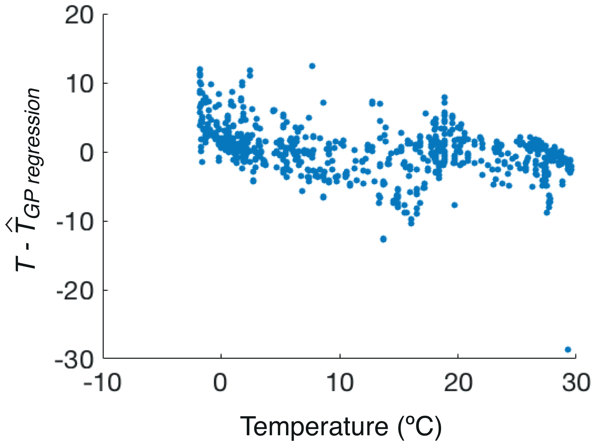
Figure 5 The error of the GPR (Gaussian process regression) predictor as a function of the true temperature.

2.5 Data structure

The random forest (Sect. 2.3) and GPR approaches (Sect. 2.4) are agnostic about any underlying bio-physical model that might impart the observed temperature dependence on GDGT relative abundances produced by archaea. They are essentially optimised interpolation tools for mapping correlations between temperature and GDGT abundances within the range of the modern calibration dataset; they can make no sensible inference about the behaviour of this relationship outside of the range of this training data. To move from interpolation within, to extrapolation beyond, the modern calibration requires an understanding of, and model for, the temperature dependence of GDGT production. To explore these relationships and the extent to which the ancient and modern data reside in a coherent relationship within GDGT space, we employed two forms of dimensionality reduction to enable visualisation of the data in two or three dimensions. The fundamental point is that if temperature is the dominant control, all of the data should lie approximately on a one-dimensional curve in GDGT space, and the arclength along this curve should correspond to temperature; we will revisit this point below.

We first employed a version of principal component analysis (PCA) tailored to compositional data (Aitcheson, 1982, 1983; Aitcheston and Greenacre, 2002; Filzmoser et al., 2009a, b, 2012). Taking into account the compositional nature of the data is important because the sum-to-one constraint induces correlations between variables which are not accounted for by classical PCA. Furthermore, apparently nonlinear structure in Euclidean space often corresponds to linearity in the simplex (i.e. the restricted space in which all elements sum to one) (Egozcue et al., 2003). Figure 6 shows the modern, Eocene and Cretaceous data projected onto the first two principal components. Aside from the obvious outlying cluster of Cretaceous data, characterised by GDGT-3 fractions above 0.6, the bulk of the data occupy a two-dimensional point cloud with a small amount of curvature. The large majority of the Cretaceous data has more positive PC1 values relative to the modern data.

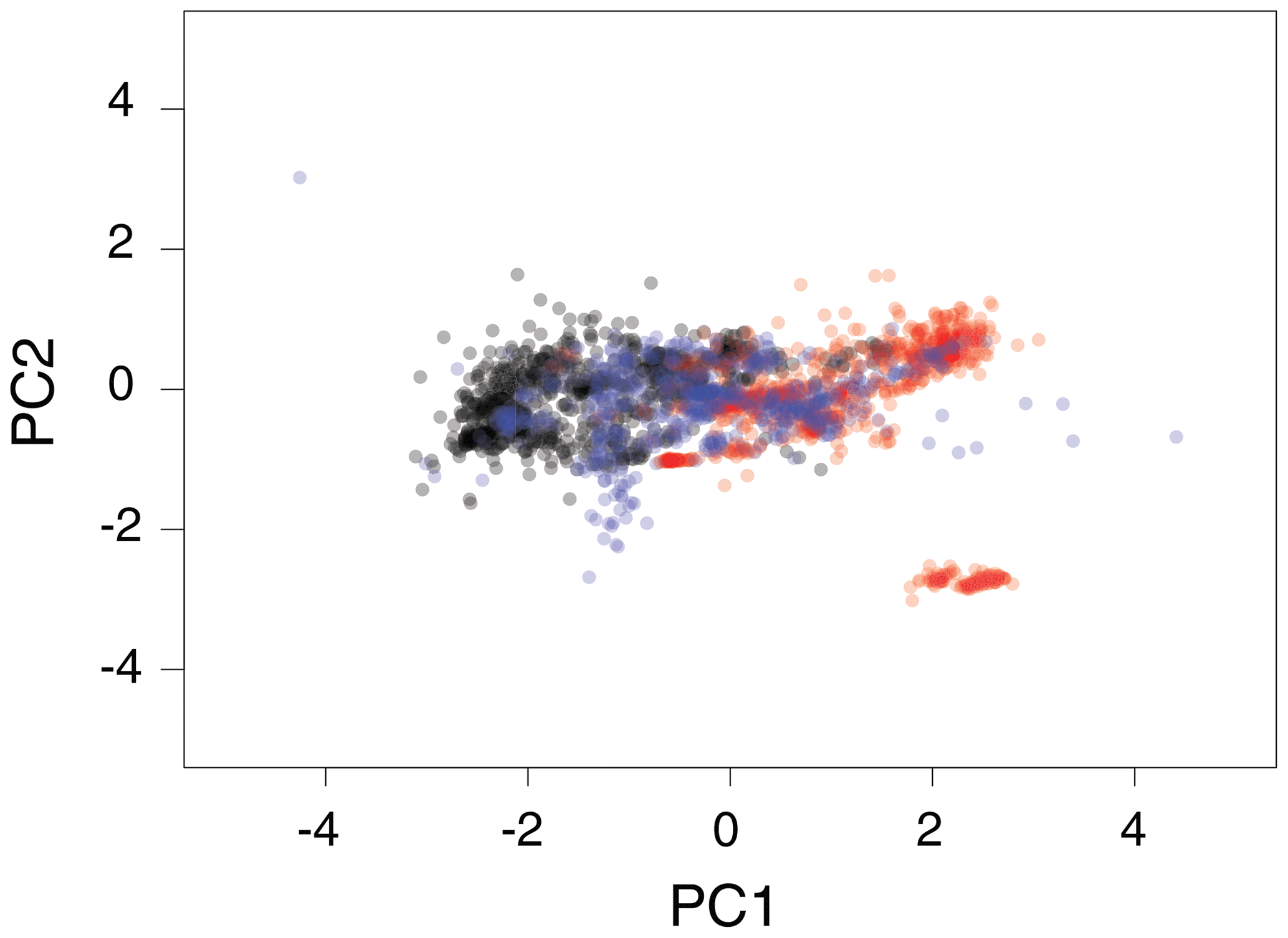
Figure 6 Modern and ancient data projected onto the first two compositional principal components. Black: modern; blue: Eocene (Inglis et al., 2015); red: Cretaceous (O'Brien et al., 2017).

We also explored the data using diffusion maps (Coifman et al., 2005; Haghverdi et al., 2015), a nonlinear dimensionality reduction tool designed to extract the dominant modes of variability in the data. Such diffusion maps have been successfully used to infer latent variables that can explain patterns of gene expression. In the case of biological organisms, this latent variable is commonly developmental age (called pseudo-time) (Haghverdi et al., 2016). In our case, the assumption would be that this latent variable corresponds to temperature. Inspection of the eigenvalues of the diffusion map transition matrix suggests that four diffusion components are adequate to represent the data; we plot the second, third and fourth of these components in Fig. 7 for the modern and ancient data. The separate clusters marked “A” are the outlying Cretaceous points with high GDGT-3 values. The bulk of the modern data lies on the branch marked “B”, while the bulk of the Cretaceous data lies on the branch marked “C”. Notably, the majority of the modern points lying on branch C are from the Red Sea, which suggests that the Red Sea data are essential for understanding ancient climates (particularly Cretaceous climates).

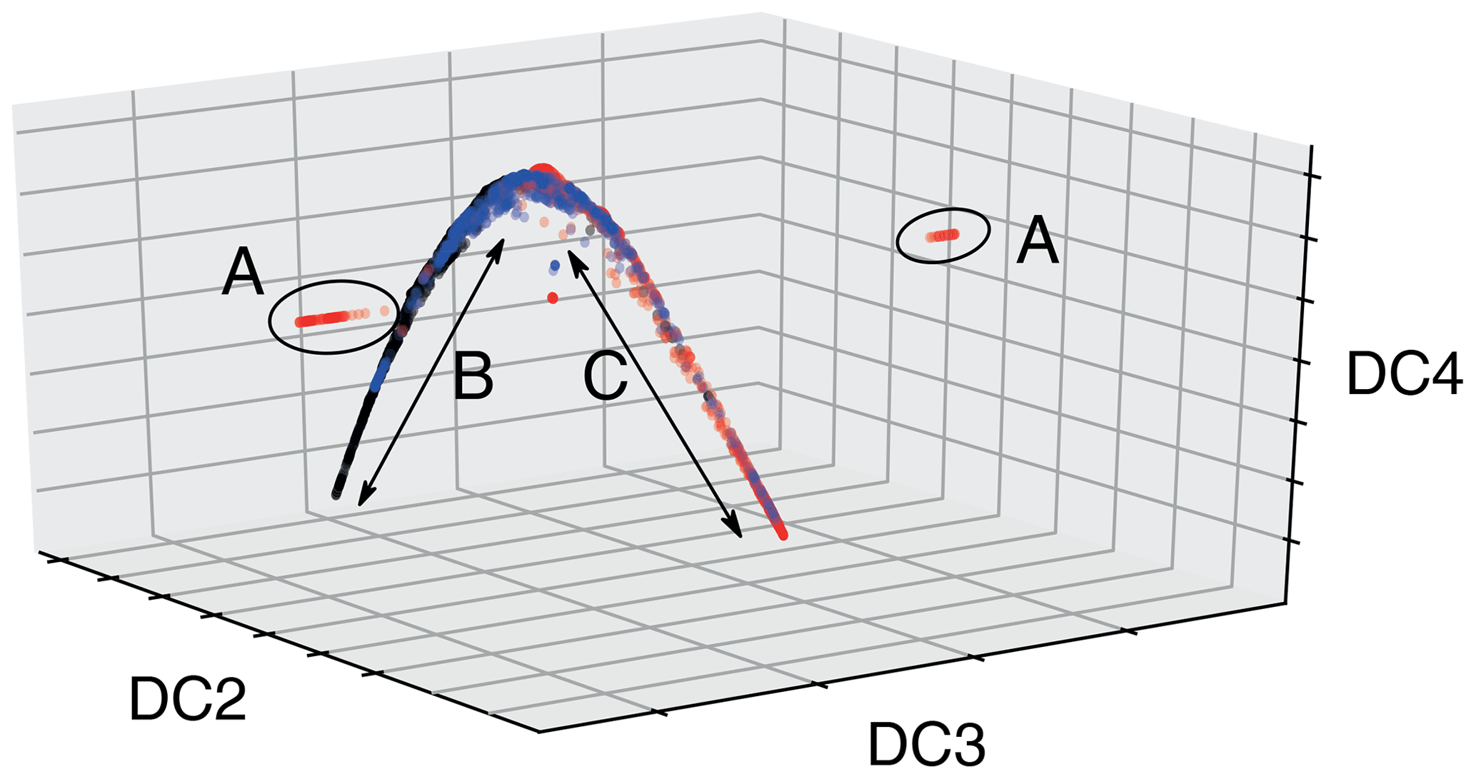
Figure 7 Diffusion map projection of the modern and ancient data. Black: modern; blue: Eocene (Inglis et al., 2015); red: Cretaceous (O'Brien et al., 2017). Separate clusters marked “A” are the outlying Cretaceous points with high GDGT-3 values. Branch “B” is dominated by modern data points; branch “C” by Cretaceous data.

The relationship between the first diffusion component and TEX₈₆ for all data is shown in Fig. 8. There is a clear correlation, despite the presence of some outlying Cretaceous points, some of which are not shown because they lie so far outside the majority data range within this projection. This suggests that TEX₈₆ is, in one sense, a natural one-dimensional representation of the data. We also plot the first diffusion component for the modern data as a function of temperature (Fig. 9). We see a similar pattern emerging to that displayed by TEX₈₆ – there is little sensitivity to temperature below 15 ^∘C, and between ∼ 20 and 25 ^∘C. An interesting avenue for future research might be to explore the temperature–GDGT system from a dynamical systems perspective, i.e. use simple mechanistic mathematical models to explore the temperature dependence of steady-state GDGT distributions. It may be that such models suggest that only a few steady states exist, and that temperature is a bifurcation parameter, i.e. it controls the switch between the steady states. Note also the downward slope in the residual pattern in Fig. 4 between 0 and 15–17 ^∘C, and again at higher temperatures. This pattern is consistent with predictions that are biased towards the centre of each “cluster”, i.e. a system which is not very sensitive to temperature but can distinguish between high and low temperatures reasonably well. This observation also links to recent culture studies (Elling et al., 2015) and Pliocene–Pleistocene sapropel data (Polik et al., 2018), which support the existence of discrete populations with unique GDGT–temperature relationships and that temporal changes in population over time can drive changes in TEX₈₆.

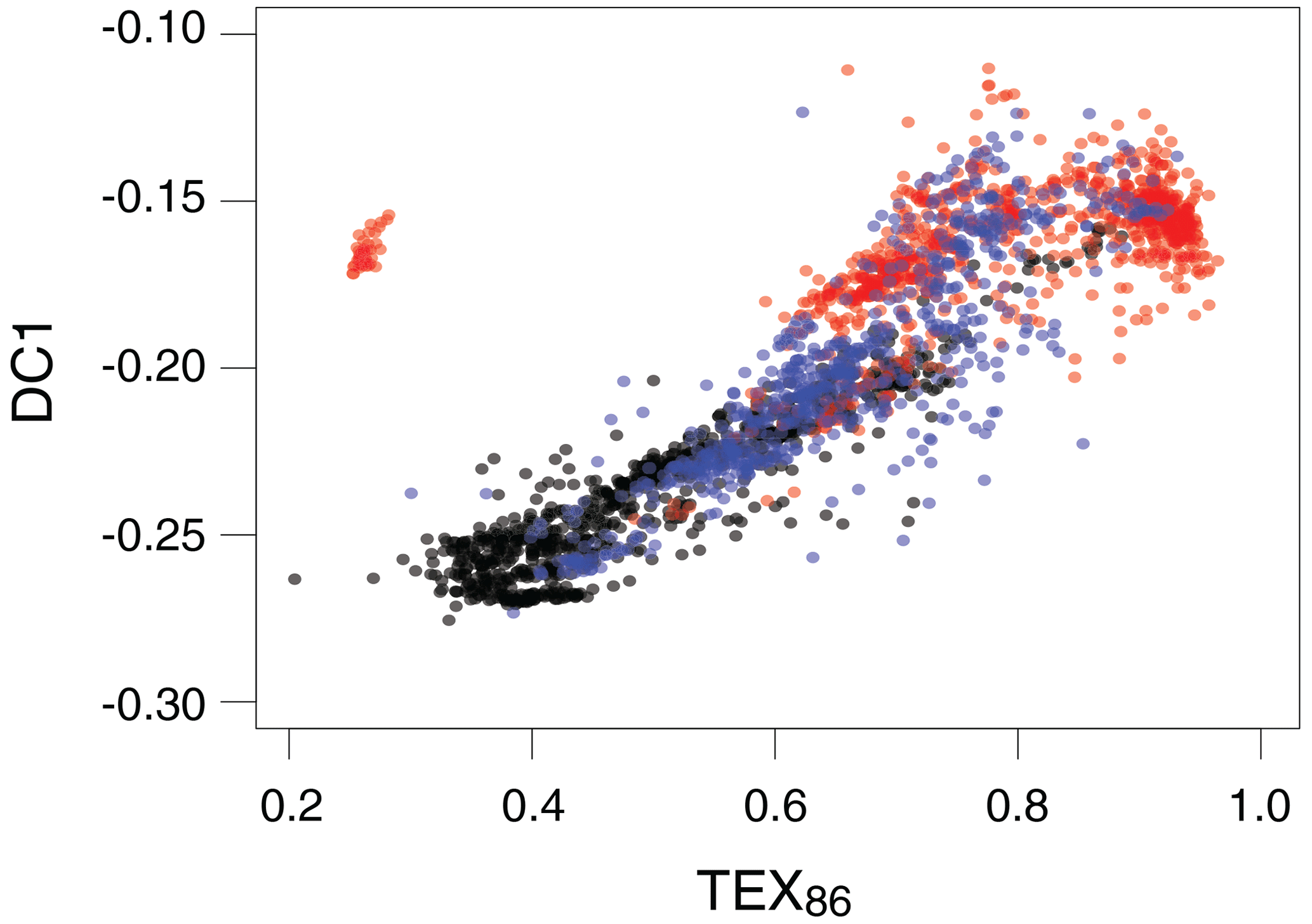
Figure 8 The first diffusion component as a function of TEX₈₆. Some outlying points have been excluded from the plot for the purposes of visualisation. Black: modern; blue: Eocene (Inglis et al., 2015); red: Cretaceous (O'Brien et al., 2017).

Figure 9 The first diffusion component as a function of temperature (modern data only).

2.6 Forward modelling

Based on the analysis of the combined modern and ancient data structure outlined above, there appears to be some consistency to underlying trends in the overall variance of GDGT relative abundances. These trends provide some hope that models of this variance, and its relationship to sea surface temperature, within the modern dataset could be developed to predict ancient SSTs. TEX₈₆ and BAYSPAR are such models, but they are limited by, first, the reduction of six-dimensional GDGT space to a one-dimensional index, and second, by an ad hoc model choice – linear, exponential – that does not account for uncertainty in model fit to the modern calibration data, and the resultant uncertainty in the estimation of ancient SSTs relating to model choice. To overcome these issues, we develop a forward (Fwd) model based on a multi-output Gaussian process (Alvarez et al., 2012), which models GDGT compositions as functions of temperature, accounting for correlations between GDGT measurements. This model is then inverted to obtain temperatures which are compatible with a measured GDGT composition. In simple terms, we posit that a measured GDGT composition is generated by some unknown function of temperature and corrupted by noise, which may be due to measurement error or some unmodelled particularity of the environment in which the sample was generated. We proceed by defining a large (in this case infinite) set of functions of temperature to explore and compare them to the available data, throwing away those functions which do not adequately fit the data. This means, of course, that the behaviour of the functions we accept is allowed to vary more widely outside the range of the modern data than within it. With no mechanistic underpinning, choosing only one function (such as the inverse of TEX₈₆) based on how well it fits the modern data grossly underestimates our uncertainty about temperature where no modern analogue is available.

The forward modelling approach is similar to that of Haslett et al. (2006), who argue that it is preferable to model measured compositions as functions of climate, before probabilistically inverting the model to infer plausible climates given a composition. The cost of modelling the data in this more natural way is the loss of degrees of freedom – we are now attempting to fit a one-dimensional line through a multidimensional point cloud rather than fit a multidimensional surface to the GDGT data, which means that the predictive power of the model suffers, at least on the modern data. The existing BAYSPAR calibration also specifies the model in the forward direction; however, while BAYSPAR does model spatial variability, it assumes a monotonic relationship between TEX and SST, only accounting for uncertainties on the parameters within the model rather than any systematic uncertainty in the model itself. As with all GP models, the choice of kernel has a substantial impact on predictions (and their associated uncertainty) outside the range of the modern data, where predictions revert to the prior implied by the kernel. Given that we have no mechanistic model for the data-generating process, we recommend the use of kernels which do not impose strong prior assumptions on the form of the GDGT–temperature relationship (e.g. kernels with a linear component) and thus reasonably represent model uncertainty outside the range of the modern data. We choose a zero-mean Matérn 3∕2 kernel for the applications below. Note, however, that since we are working in isometric log-ratio transformed coordinates, this corresponds to a prior assumption of uniform compositions at all temperatures, i.e. all components are equally abundant.

The residuals for the forward model are shown in Fig. 10. The clear pattern in the residuals does not necessarily indicate model misspecification, since no explicit noise model is specified for temperatures. Predictive distributions are to be interpreted in the Bayesian sense, in that they represent a “degree of belief” in temperatures given the model and the modern data. The residual pattern is similar to that of the random forest (Fig. 4) with two clear downward slopes, suggesting again that the data are clustered into temperatures above and below 16–17 ^∘C, and that predictions tend towards temperatures at the centres of these clusters.

Figure 10 Temperature residuals for the forward model.

An advantage of the forward modelling approach is that the inversion can incorporate substantive prior information about temperatures for individual data points. In particular, other proxy systems can be used to elicit prior distributions over temperatures to constrain GDGT-based predictions, particularly when attempting to reconstruct ancient climates with no modern analogue in GDGT space. We emphasise that outside the range of the modern data, the utility of the models is almost solely due to the prior information included in the reconstruction. At present, the only priors being used in the forward model prescribe a reasonable upper limit and lower limit on temperatures (see Supplement). The only way to improve these reconstructions will be for future iterations to incorporate prior information from other proxies. It is worth noting that the predictive uncertainty, while reasonably well-described by the standard deviation in cases where ancient data lie quite close to the modern data in GDGT space, can be highly multimodal (Fig. 11). This is the case when estimates are significantly outside of the modern calibration dataset, such as low-latitude data in the Cretaceous, or where there is considerable scatter in the modern calibration data, for example in the low temperature range (< 5 ^∘C).

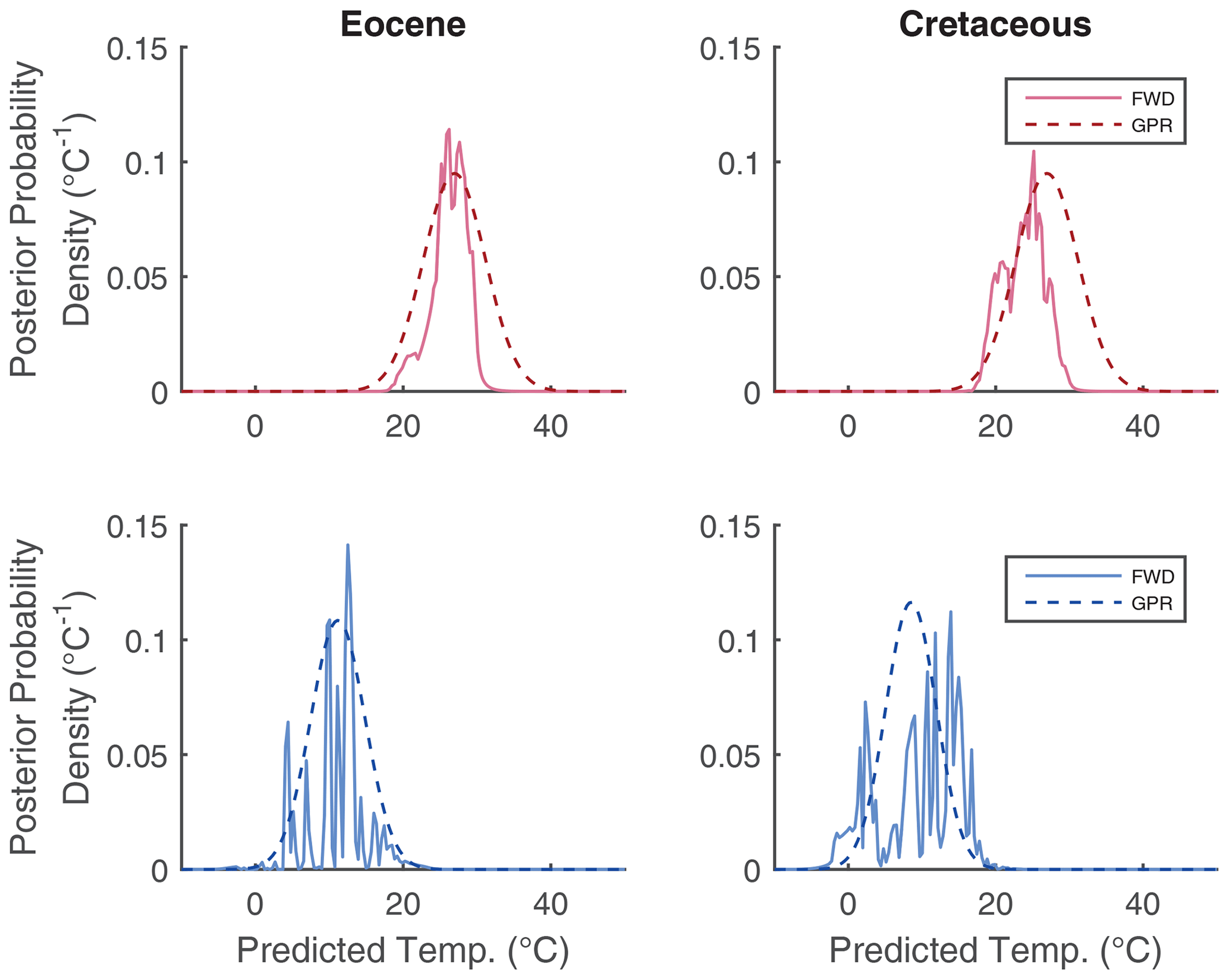
Figure 11 The posterior distributions over temperature from the forward model for selected examples of high and low temperature examples, from both the Eocene and Cretaceous. The Gaussian error envelope from the GPR model is shown for comparison.

3 Non-analogue behaviour and extrapolation

In principle, the predictors described above can be applied directly to ancient data, such as data from the Eocene or Cretaceous (Inglis et al., 2015; O'Brien et al., 2017). In practice, one should be careful with using models outside their domain of applicability. The machine learning tools described above, which are ultimately based on the analysis of nearby calibration data in GDGT space, are fundamentally designed for interpolation. To the extent that ancient data occupy a very different region in GDGT space, extrapolation is required, which the models do not adequately account for. The divergence between modern calibration data and ancient data is evident from Fig. 12, which shows histograms of minimum normalised distances between “high-quality” Eocene and Cretaceous data points (those that passed the screening tests applied by O'Brien et al., 2017 and Inglis et al., 2015) and the nearest point in the full modern dataset. We strongly recommend the use of the weighted distance metric (D_nearest) as a screening method to determine whether the modern core-top GDGT assemblage data is an appropriate basis for ancient SST estimation on a case-by-case basis. Note that this distance measure is weighted by the scale length of the relevant parameter as estimated by the Gaussian process emulator in order to quantify the relative position of ancient GDGT assemblages to the modern core-top data. By using the GP-estimated covariance as the distance metric, we account for the sensitivity of different GDGT components to temperature. Our inference is that samples with D_nearest > 0.5 are unlikely to be well constrained by any current calibration model. In these instances, in both our GPR and Fwd models, the constraints provided by the modern calibration dataset are such that estimates of temperature have large uncertainty bands that are dictated by model priors, i.e. are unconstrained by the calibration data (e.g. Figs. 13 and 14). This uncertainty is not apparent from estimates generated by BAYSPAR or ${\text{TEX}}_{\mathrm{86}}^{\text{H}}$ models, although the underlying lack of constraints are the same. While 93 % of validation data points in the modern data have D_nearest < 0.5, this is the case for only 33 % of Eocene samples and 3 % of Cretaceous samples.

Figure 12 A histogram of normalised distances to the nearest sample in the modern dataset for Eocene and Cretaceous data, excluding samples that had been screened out in previous compilations using BIT, MI and RI following the approach of Inglis et al. (2015) and O'Brien et al. (2017).

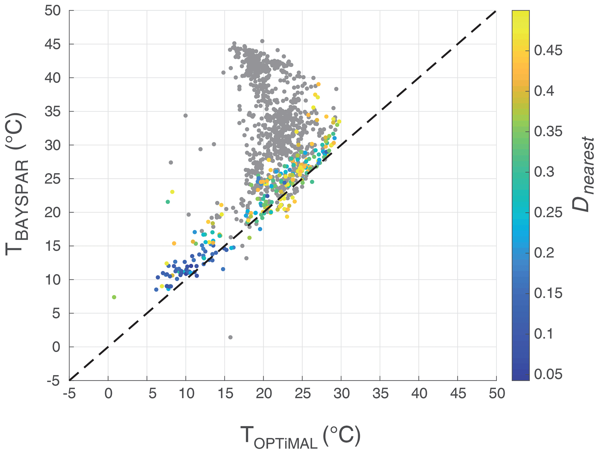
Figure 13 Comparison of temperature estimates for the BAYSPAR and the OPTiMAL GPR model. Greyed-out data fails the D_nearest test (> 0.5), and the colour scaling reflects D_nearest values for those data points that pass. Note that outside of the constraints of the modern calibration (training) dataset (D_nearest test > 0.5) the GPR model temperature estimates revert to the mean value of the calibration dataset, with an uncertainty that reverts to the standard deviation of the training data.

Figure 14 Inter-comparison of temperature estimates and standard errors (y axis) for compiled Eocene and Cretaceous data calculated using OPTiMAL (a) and BAYSPAR (b). Greyed-out data fails the D_nearest test (> 0.5), and the colour scaling reflects D_nearest values for those data points that pass. The black dashed line shows the D_nearest threshold (> 0.5).

Where ancient GDGT distributions lie far from the modern calibration dataset (D_nearest > 0.5), we argue that there is no suitable set of modern analogue GDGT distributions from which to infer growth temperatures for this ancient GDGT distribution. Both the GPR and Fwd models revert to imposed priors once the distance from the modern calibration dataset increases. We also note that there are two broad, non-mutually exclusive categories of samples that lie far from the modern calibration dataset (D_nearest > 0.5): the first are samples that seem to lie “beyond” the temperature–GDGT calibration relationship, likely with (unconstrained) GDGT formation temperatures higher than the modern core-top calibrations; the second are samples with anomalous GDGT distributions lying on the margins of, or far away from, the main GDGT clustering in six-dimensional space (see outliers in Fig. 8).

Given the (current) limit on natural mean annual surface ocean temperatures of ∼ 30 ^∘C, extending the GDGT–temperature calibration might be possible through (1) integration of full GDGT abundance distributions produced in high-temperature culture, mesocosm or artificially warmed sea surface conditions into the models followed by (2) validation through robust inter-comparisons of any new GDGT palaeothermometer for high-temperature conditions with other temperature proxies from past warm climate states. As discussed in the introduction, the first approach is limited by the ability of culture or mesocosm experiments to accurately represent the true diversity and growth environments and dynamics of natural microbial populations. Such studies clearly indicate a more complex, community-scale control on changing GDGT relative abundances to growth temperatures (e.g. Elling et al., 2015). Community-scale temperature dependency can be modelled relatively well with analyses of natural production preserved in core-top sediments, especially with more sophisticated model fitting, including the GPR and Fwd model presented here. Above ∼ 30 ^∘C, however, the behaviour of even single strains of mesophilic archaea are not well-constrained by culture experiments, and the natural community-level responses above this temperature are, so far, unknown. While there is evidence for the temperature sensitivity of GDGT production by thermophilic and acidophilic archaea in older papers (de Rosa et al., 1980; Gliozzi et al., 1983), recent works, characterised by more precise phylogenetic and culturing techniques, show a more complex relationship between GDGT production and temperature. Elling et al. (2017) highlight that there is no correlation between TEX₈₆ and growth temperature in a range of phylogenetically different thaumarchaeal cultures – including thermophilic species. Bale et al. (2019) recently cultured Candidatus Nitrosotenuis uzonensis from the moderately thermophilic order Nitrosopumilales (that contains many mesophilic marine strains). They found no correlation between TEX₈₆ calibrations (either the Kim et al., 2010, core-top or Wuchter et al., 2004, and Schouten et al., 2008, mesocosm calibrations) with membrane lipid composition at different growth temperatures (37, 46 and 50 ^∘C) and found that phylogeny generally seems to have a stronger influence on GDGT distribution than temperature. In view of these existing data, extrapolation of modern core-top calibration datasets into the unknown above 30 ^∘C is uncertain, although the coherent patterns apparent across GDGT space, between modern, Eocene and Cretaceous data (Fig. 7), do provide some grounds for hope that the extension of GDGT palaeothermometry beyond 30 ^∘C might be possible in future.

4 OPTiMAL and D_nearest: a more robust method for GDGT-based palaeothermometry

A more robust framework for GDGT-based palaeothermometry could be achieved with a flexible predictive model that uses the full range of six GDGT relative abundances and has transparent and robust estimates of the prediction uncertainty. In this context, the Gaussian process regression model (GPR; Sect. 2.4) outperforms the forward model (Fwd; Sect. 2.6) within the modern calibration dataset and we recommend standard use of the GPR model, henceforth called OPTiMAL, over the Fwd model. Model code for the calculation of D_nearest values and OPTiMAL SST estimates (MATLAB script) and the Fwd model SST estimates (R script) are archived in the Zenodo repository, https://doi.org/10.5281/zenodo.4293851 (Greene and Mandel, 2020).

Following Tierney and Tingley (2014) we use a reduced calibration dataset, with the exclusion of Arctic data with observed SSTs of less than 3 ^∘C (“NoNorth/TT13” of Tierney and Tingley, 2014) but with the inclusion of additional core-top data from Seki et al. (2014). Full details of this calibration dataset are provided in the Supplement; to distinguish from the original OPTiMAL calibration data, which included the Arctic data < 3 ^∘C, we refer to the original data as “Op1” and the new calibration dataset as “Op3”. An “Op2” is also available, which is the same as Op1 except that it excludes the Seki et al. (2014) data. In sensitivity tests to a range of applications across Quaternary and deep-time datasets, calibration Op1 and Op2 performed in almost identical fashion. The performances of Op1 and Op3 were very similar in most applications, except in applications to the palaeo-Arctic (see below), where the inclusion of modern Arctic calibration data (Op1) provided closer calibration constraints to the palaeo-data. Although the inclusion of modern Arctic data may well be beneficial for the study of high-latitude palaeoclimate archives, we are initially cautious as in this instance the deep-time palaeo-data have previously been rejected because of a potential bias by non-marine inputs indicated by high BIT indices (Sluijs et al., 2020). In this case there could be some consistency between the modern and ancient GDGT production by marine archaea in the Arctic which may help in the understanding of GDGT-based palaeothermometry in this unusual environment (Sluijs et al., 2020), but we recommend further investigation of the modern Arctic core-top biomarker assemblages before their regular inclusion into the calibration dataset. The D_nearest methodology may prove useful in quantifying analogue and non-analogue behaviour through time in such conditions. For the purposes of this study, however, we take the conservative approach, and one that maintains a more consistent calibration basis with BAYSPAR, by using OPTiMAL calibration Op3 in the remainder of this discussion, and recommend its use in future applications of OPTiMAL.

To investigate the behaviour of the new OPTiMAL model, we compare temperature predictions including uncertainties for the Eocene and Cretaceous datasets, made by OPTiMAL and the BAYSPAR methodology of Tierney and Tingley (2014) (Figs. 13 and 14), using the default priors specified in the model code for the BAYSPAR estimation. The OPTiMAL model systematically estimates slightly cooler temperatures than BAYSPAR, with the biggest offsets below ∼ 15 ^∘C (Fig. 13). Fossil GDGT assemblages that fail the D_nearest test are shown in grey, which clearly illustrate the regression to the mean in the OPTiMAL model, whereas BAYSPAR continues to make SST predictions up to and exceeding 40 ^∘C for these “non-analogue” samples due to the fact that BAYSPAR assumes that higher TEX₈₆ values equate to higher temperatures as part of the functional form of the model, whereas the GPR model is agnostic on this. A comparison of error estimation between OPTiMAL and BAYSPAR is shown in Fig. 14. For most of the predictive range below the D_nearest cut-off of 0.5, OPTiMAL has smaller predicted uncertainties than BAYSPAR, especially in the lower temperature range. As D_nearest increases, i.e. as the fossil GDGT assemblage moves further from the constraints of the modern calibration dataset, the error on OPTiMAL increases, until it reaches the standard deviation of the modern calibration dataset (i.e. is completely unconstrained). In other words, OPTiMAL generates maximum-likelihood SSTs with robust confidence intervals, which appropriately reflect the relative position of an ancient sample used for SST estimation and the structure of the modern calibration dataset. Where there are strong constraints from near analogues in the modern data, uncertainties will be small; where there are weak constraints, uncertainty increases. In contrast, while uncertainty bounds do increase when BAYSPAR is used to extrapolate beyond the modern calibration, they are not as large as OPTiMAL because BAYSPAR assumes a linear increase in SST at higher TEX values.

We also provide an initial assessment of the inter-relationship between standard screening indices and D_nearest, for the Eocene and Cretaceous compilations, where the data are available to calculate these measures (Fig. 15). For ease of comparison between Eocene and Cretaceous datasets and visualisation of the majority of the data, extreme outliers (D_nearest > 4.0) are not shown. The metrics include the BIT index (Hopmans et al., 2004; Weijers et al., 2011), the methane index (MI; Zhang et al., 2011), the deviation between TEX₈₆ and the ring index (ΔRI; Zhang et al., 2016) and the %GDGT-0 (Blaga et al., 2009; Sinninghe Damsté et al., 2012). The standard screening levels for each of these metrics, as used in previous palaeo-compilations (O'Brien et al., 2017), are shown in the blue shaded areas in Fig. 15 (BIT > 0.5; MI > 0.5; ΔRI > 0.3; %GDGT-0 > 67%) – data points within these areas fail the standard screening. Also shown in Fig. 15 is the region where data pass our D_nearest screening requirement (grey shaded vertical region). In nearly all cases GDGT assemblages that fail these traditional screening tests also have D_nearest values that exceed 0.5 – i.e. “abnormal” GDGT assemblages are well-screened by D_nearest. The main exception to this is the BIT index in the Eocene dataset, where 15 samples have high BIT values (> 0.5) but have GDGT assemblages that are close to modern analogues in the calibration dataset (D_nearest < 0.5). Of these samples, 9 are from the Arctic Ocean between the Paleocene–Eocene thermal maximum (PETM) and Eocene thermal maximum 2 (ETM2), an interval noted for its relatively high BIT index values (Sluijs et al., 2020); 3 are from the Eocene–Oligocene transition of ODP Site 1218 (eastern Equatorial Pacific) (Liu et al., 2009); 2 are from the middle Eocene of Seymour Island (Douglas et al., 2014); and 1 is from the late Eocene of DSDP Site 511, which has been already noted as an individual sample with anomalously high BIT in this dataset (Liu et al., 2009; Inglis et al., 2015). Although high BIT at ODP Site 1218 has been inferred to represent “relatively high terrestrial input” (Inglis et al., 2015) this seems unusual for a fully pelagic site situated on oceanic crust > 3000 km away from the nearest continental landmass. Interpreting high BIT values as exclusively caused by terrestrial organic components appears problematic in this instance, especially as D_nearest < 0.5 give some assurance that these GDGT assemblages from ODP Site 1218 are well-modelled by the modern calibration dataset. GDGT assemblages from Seymour Island associated with high BIT values (> 0.4) appear to have an impact on the TEX${}_{\mathrm{86}}^{\text{H}}$ SST proxy (Inglis et al., 2015), but the 2 samples that fail BIT (> 0.5) but pass D_nearest (< 0.5) give OPTiMAL SSTs consistent (5–6 ^∘C) with the SSTs from samples that pass all other screening and D_nearest (∼ 4–7 ^∘C). In summary, the relationship between D_nearest and BIT suggests that BIT is not always closely coupled to GDGT assemblages that are strongly divergent from the modern calibration dataset.

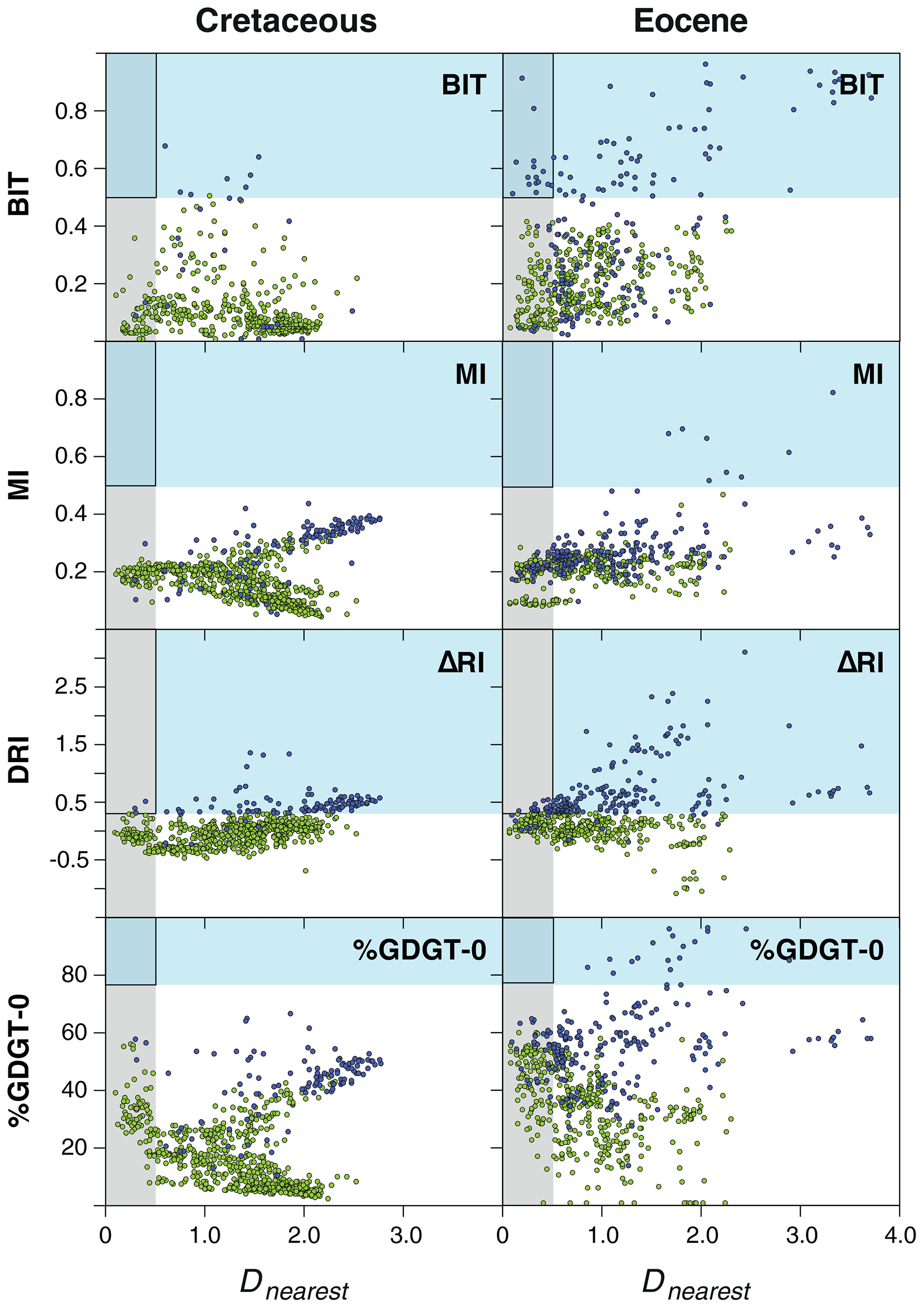
Figure 15 Comparison of D_nearest against standard screening indices: BIT and MI indices, ΔRI and %GDGT-O for the Eocene (Inglis et al., 2015) and Cretaceous (O'Brien et al., 2017) datasets. Blue shaded regions show the standard failure thresholds for these indices (see text); grey shaded region highlights data that are below the D_nearest threshold of 0.5. Data points that fail any one of the standard screening indices are shown in blue, and data points that pass all standard screening indices are shown in green. The outlined black box is the region of data that fails traditional screening indices but passes D_nearest (< 0.5).

With respect to the other screening indices there are clear indications that increased distance from the modern calibration (increased D_nearest) is associated with a trend towards the “thresholds of failure” in the screening indices. This pattern is most clear with the ΔRI in both the Cretaceous and the Eocene data, as increasing numbers of samples fail ΔRI as D_nearest increases. This supports ΔRI as a robust methodology for identifying samples that strongly diverge from the expected temperature dependence of GDGT assemblages as modelled by TEX₈₆ in the modern calibration dataset. There are, however, samples that pass D_nearest < 0.5 but fail ΔRI in both the Eocene and Cretaceous datasets – these must have “near neighbours” in the modern calibration data but yet have a temperature sensitivity that is less well-modelled by TEX₈₆ (divergence between RI and TEX₈₆). Conversely there are many Eocene and Cretaceous data points with ΔRI < 0.3, but which fail D_nearest (> 0.5). These data most likely represent GDGT assemblages formed at high temperatures, beyond the range of the modern calibration data.

To investigate these behaviours requires the publication of the full range GDGT abundance data. Whilst key compilations of Eocene and Cretaceous GDGT data have strongly encouraged the release of such datasets (Lunt et al., 2012; Dunkley Jones et al., 2013; Inglis et al., 2015; O'Brien et al., 2017), most Neogene studies only publish TEX₈₆ values. Without full GDGT assemblage data neither OPTiMAL nor other detailed assessments of GDGT behaviour and type can be made, and we would strongly encourage authors, reviewers and editors to ensure the publication of full GDGT assemblages in future.

.

Figure 16 Late Pleistocene to Holocene GDGT-derived OPTiMAL palaeotemperatures compared to BAYSPAR and $U_{\mathrm{37}}^{k^{\prime }}$ SSTs. Shaded regions represent reported 5th and 95th percentile confidence intervals. (a) Eastern Mediterranean data from core GeoB 7702-3 (Castañeda et al., 2010); (b) South China Sea data from ODP Site 1146 (Thomas et al., 2014)

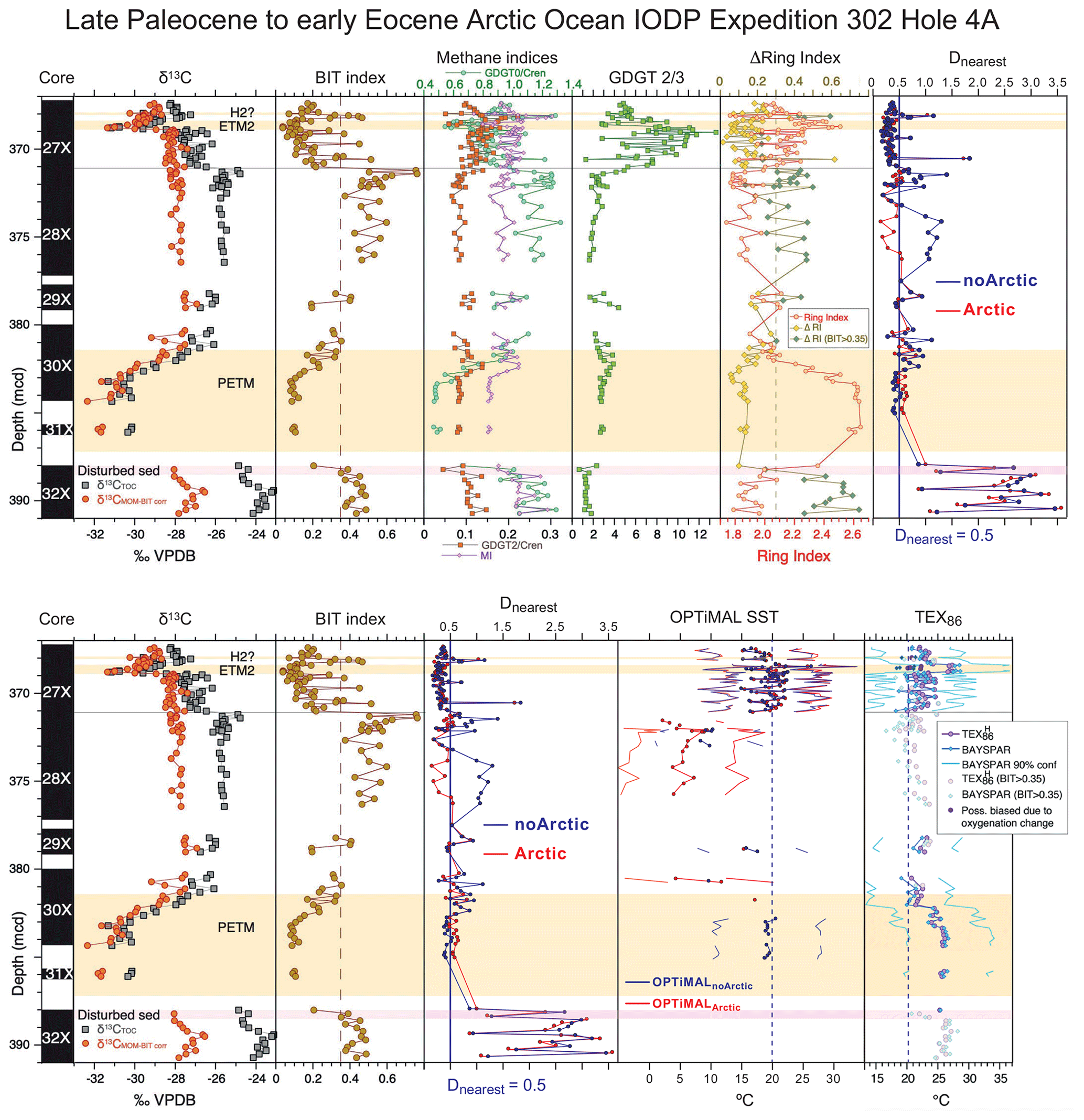
Figure 17 Comparison of GDGT screening indices, TEX${}_{\mathrm{86}}^{\text{H}}$, BAYSPAR and OPTiMAL SSTs from the Arctic Site IODP Expedition 302 Hole 4A. Depths are metres composite depth (mcd). Data and figures modified from the most recent reassessment by Sluijs et al. (2020).

Finally, to test the behaviour of OPTiMAL within established SST time series, we provide three examples: two from the late Pleistocene to Holocene (Fig. 16) and one from the Eocene (Fig. 17). For the Pleistocene to Holocene examples OPTiMAL SSTs are shown against estimates from BAYSPAR and the alkenone-based $U_{\mathrm{37}}^{k^{\prime }}$ temperature proxy. The first of these time series is from GeoB 7702-3 in the eastern Mediterranean and spans the last 26 kyr, including data spanning Termination I (Castañeda et al., 2010). The second is from ODP Site 1146 in the South China Sea and spans the last 350 kyr (Thomas et al., 2014). In both records the long-term dynamics are consistent between the independent $U_{\mathrm{37}}^{k^{\prime }}$ SST proxy and both BAYSPAR and OPTiMAL. In the eastern Mediterranean OPTiMAL SSTs are slightly cooler in the glacial era and warmer in the Holocene than the other proxies. In the South China Sea, OPTiMAL is again cooler than BAYSPAR during glacial intervals but at this location is in closer agreement than BAYSPAR with the $U_{\mathrm{37}}^{k^{\prime }}$ SST proxy through most of the record.

The final example is from the latest Paleocene to early Eocene of IODP Expedition 302 Hole 4A on Lomonosov Ridge (Sluijs et al., 2006, 2009, 2020). This site is useful as it has been the focus of detailed reassessment and reanalysis, using most of the available screening methodologies to detect aberrant GDGT assemblages (Sluijs et al., 2020). Here we use this recently published data to compare the new D_nearest screening metric against multiple other screening protocols (Fig. 17). We also show both D_nearest values and OPTiMAL SST estimates for two models – one with modern Arctic data with SST < 3 ^∘C included in the calibration (OPTiMAL_Arctic; equivalent to calibration dataset Op1 presented in this paper) and one with this data excluded (OPTiMAL_noArctic; equivalent to the new calibration dataset Op3). It is clear from the pattern of D_nearest for these two options that the inclusion of modern Arctic data provides more calibration data that are closer to the Eocene palaeo-Arctic, to the extent that substantially more samples pass the D_nearest < 0.5 constraint, especially in pre-ETM2 interval from ∼ 372 to 376 mcd (metres composite depth). This interval contains, however, samples with the highest BIT values of the succession (> 0.4), and elevated ΔRI (> 0.3). With these other “warning signs” concerning the reliability of GDGT assemblages for SST estimation in this interval, the relatively low D_nearest values are most likely to represent some similarity in the non-thermal controls on GDGT assemblages between the modern and palaeo-Arctic. More work needs to be done to constrain the reliability of temperature dependence and archaeal GDGT production in these modern high-latitude systems so that we can have confidence in their inclusion in calibration datasets for palaeo-SST estimation. It is on this basis that we recommend users of OPTiMAL use the the “noArctic” (Op3) calibration as the default. The OPTiMAL methodology does, however, offer a simple means to integrate new robust calibration data, and a method to explore the distance relationships between modern and ancient GDGT production.

Considering the “noArctic” D_nearest and OPTiMAL SSTs for Exp. 302 Hole 4A, it is clear that of all the screening methods, D_nearest shows the strongest similarity to ΔRI – with high (“failure”) values in the pre-PETM and then again between ∼ 371 and 376 mcd, and even picking up the same short-lived “failure” intervals, or spikes, between 368 and 371 mcd. SST estimates based on OPTiMAL show broadly similar trends to TEX${}_{\mathrm{86}}^{\text{H}}$ and BAYSPAR, with a warm PETM, cooling post-PETM and then warming again into ETM2. It should be noted, however, that peak temperatures for OPTiMAL are ∼ 5 ^∘C cooler than TEX${}_{\mathrm{86}}^{\text{H}}$ and BAYSPAR (e.g. PETM SSTs < 20 ^∘C for OPTiMAL and > 25 ^∘C for TEX${}_{\mathrm{86}}^{\text{H}}$ and BAYSPAR) and show more cooling post-PETM, with SST estimates of ∼ 10 ^∘C (OPTiMAL_noArctic) as opposed to ∼ 20 ^∘C for TEX${}_{\mathrm{86}}^{\text{H}}$ and BAYSPAR.

5 Conclusions

The use of GDGT abundances to estimate temperatures in clearly non-analogue conditions is, at present, problematic on the basis of the available calibration constraints or a good understanding of underlying biophysical models. We hope that this study prompts further investigations that will improve these constraints for the use of GDGTs in deep-time palaeoclimate studies, where they clearly have substantial potential as temperature proxies. Temperature estimates based on fossil GDGT assemblages that are within range of, or similar to, modern GDGT calibration data, do, however, rest on a strong, underlying temperature dependence observed in the empirical data.

In this study, we apply modern machine learning tools, including Gaussian process emulators and forward modelling, to improve temperature estimation and the representation of uncertainty in GDGT-based SST reconstructions. Using our new nearest-neighbour test, we demonstrate that > 60% of Eocene and > 90% of Cretaceous fossil GDGT distribution patterns are poorly constrained by the modern core-top calibration data. For data that do show sufficient similarity to modern data, we present OPTiMAL, a new multi-dimensional Gaussian process regression tool which uses all six GDGTs (GDGT-0, -1, -2, -3, cren and cren^′) to generate an SST estimate with associated uncertainty. The key advantages of the OPTiMAL approach are as follows: (1) these uncertainty estimates are intrinsically linked to the strength of the relationship between the fossil GDGT distributions and the modern calibration dataset, and (2) by considering all GDGT compounds in a multi-dimensional regression model it avoids the dimensionality reduction and loss of information that takes place when calibrating single parameters (TEX₈₆) to temperature. The methods presented above make very few assumptions about the data. We argue that such methods are appropriate with the current absence of any reasonable mechanistic model for the data-generating process, in that they reflect model uncertainty in a natural way. Finally, we note the potential for multi-proxy machine learning approaches, synthesising data from other palaeothermometers with independent uncertainties and biases, to improve calibration of ancient GDGT-derived SST reconstructions.