Investigating interdecadal salinity changes in the Baltic Sea in a 1850–2008 hindcast simulation

Interdecadal variability in the salinity of the Baltic Sea is dominated by a 30-year cycle with a peak-to-peak amplitude of around 0.4 g kg⁻¹ at the surface. Such changes may have substantial consequences for the ecosystem, since species are adapted to a suitable salinity range and may experience habitat shifts. It is therefore important to understand the drivers of such changes. We use both analysis of empirical data and a numerical model reconstruction for the period of 1850–2008 to explain these interdecadal changes. The model explains 93 % and 52 % of the variance in the observed interdecadal salinity changes at the surface and the bottom, respectively, at an oceanographic station at Gotland Deep. It is known that the 30-year periodicity coincides with a variability in river runoff. Periods of enhanced runoff are followed by lower salinities. We demonstrate, however, that the drop in mean salinity cannot be understood as a simple dilution of the Baltic Sea water by freshwater. Rather, the 30-year periodicity in river runoff occurs synchronously with a substantial variation in salt water import across Darss Sill. Fewer strong inflow events occur in periods of enhanced river runoff. This reduction in the import of high-salinity water is the main reason for the freshening of the water below the permanent halocline. In the bottom waters, the variation in salinity is larger than at the surface. As a consequence, the surface layer salinity variation is caused by a combination of both effects: a direct dilution by river water and a reduced upward diffusion of salt as a consequence of reduced inflow activity. Our findings suggest that the direct dilution effect is responsible for 27 % of the salinity variations only. It remains unclear whether the covariation in river runoff and inflow activity are only a coincidental correlation during the historical period or whether a mechanistic link exists between the two quantities, e.g. whether both are caused by the same atmospheric patterns.

1 Introduction

The Baltic Sea is a brackish sea with pronounced salinity gradients, both in the horizontal and in the vertical. The narrow and shallow Danish Straits connect this marginal sea via the Kattegat to the adjacent North Sea, which allows a limited exchange of volume and salt. The brackish salinities in the Baltic Sea are the consequence of (i) a positive freshwater balance due to river runoff and net precipitation, (ii) an import of saline water across the shallow Drogden Sill and Darss Sill, and (iii) mixing processes inside the Baltic Sea.

Changes in any of these controlling factors may thus affect the Baltic Sea salinity. Major ecological consequences may result from this, since the ecosystem of the Baltic Sea is adapted to the brackish salinities and their horizontal gradient. Species diversity shows a minimum at salinities around 5–8 g kg⁻¹ (Khlebovich, 1969), since few marine species, but also few freshwater species, can adapt to these salinities. A change in Baltic Sea salinity means a regional shift in this isohaline with corresponding spatial shifts in habitats. Since a freshening of the Baltic Sea is expected in future climate due to enhanced precipitation in the catchment, these regional shifts are expected (MacKenzie et al., 2007; Vuorinen et al., 2015).

The intensity of these future changes will depend on the sensitivity of the Baltic Sea salinity to river runoff, i.e. on the vulnerability of the present-day equilibrium salinities towards changes in freshwater supply. Attributing past variations in Baltic Sea salinity is therefore essential to understand the mechanisms causing the sensitivity and, for example, discriminate between the influences of runoff and wind.

Separating the influence of runoff and wind on multidecadal salinity fluctuations in the Baltic Sea is the prerequisite for the attribution of these fluctuations to atmospheric driving mechanisms. When these fluctuations can be quantitatively explained, long-term salinity trends caused by different drivers such as sea level rise will be more easily detectable in the historical salinity record.

Both empirical and numerical model studies have assessed the effect of river runoff on Baltic Sea salinity. The studies of Winsor et al. (2001) and of Meier and Kauker (2003a) stressed that the freshwater content of the Baltic Sea showed very similar decadal fluctuations to the accumulated river runoff and net precipitation anomaly, both in phase and magnitude. A Knudsen-like model was employed by Rodhe and Winsor (2002) to explain this strong correlation (corrected in  Rodhe and Winsor, 2003). They concluded that enhanced freshwater input would lead to outflow of Baltic Sea water into the Kattegat. This would cause enhanced entrainment of low-saline water into the Kattegat deep water, which enters the Baltic Sea during inflows. A long-term change of 1 % in freshwater supply should thus lead to relative changes in salinity of more than 2 %. Their model was based on the assumption that relative variations in the barotropic flow through the Danish Straits were much smaller than those in the freshwater input and uncorrelated to them on a 5-year timescale. A steady-state model by Meier and Kauker (2003a) estimated a smaller relative salinity change of 1.6 % for a 1 % change in runoff. The model was based on the assumption that an increase in runoff leads to a small weakening of the overturning circulation only, and the analytical model results were confirmed by sensitivity experiments of a numerical model.

Another explanation for salinity changes that has been discussed is the intensity variation in westerly winds. On a timescale between 35 and 200 d, Gustafsson and Andersson (2001) found a positive correlation between (a) Kattegat sea level and salinity and (b) the north–south gradient of air pressure across the North Sea, which is directly related to westerly winds. They were able to show that the salt transports across the sills, derived by a simple conceptual model driven by this pressure gradient, partly explained the observed salinity variations. This explanation was extended by Höflich et al. (2018), who investigated events of large volume transports into the Baltic Sea, which are wind-driven. They demonstrated that the salt import during such events depends on both intensity and rapidness of the volume flow. Stagnation periods with a decade-long drop in salinity were characterized by a lack of changes in Baltic Sea volume being both large and rapid.

On a multi-year scale, in contrast, stronger westerly winds cause lower salinities (Zorita and Laine, 2000). This effect is partly related to the runoff signal, since stronger westerlies cause higher moisture transport and lead to higher precipitation in the Baltic Sea catchment. Another mechanism discussed is that the resulting barotropic pressure gradient (higher sea level in the Baltic Sea) prevents large barotropic inflows. The study of Schimanke and Meier (2016) discriminated the two effects in a stepwise multilinear regression, using a synthetic 1000-year climate model simulation as input. Here they showed that 44 % of the variance in the 10-year low-pass-filtered salinity could be explained by river runoff and precipitation alone, 23 % could be explained by zonal wind alone, and 48 % could be explained by a combination of all these drivers. This illustrates the strong interdependence between zonal wind and freshwater input.

Past salinity variations in the Baltic Sea show a prominent 30-year cycle, which has been known for decades (Malmberg and Svansson, 1982). A similar periodicity exists in river discharge of major Baltic Sea rivers (Meier and Kauker, 2003b; Gailiušis et al., 2011), and a link between both has been discussed (Malmberg and Svansson, 1982). This does, however, not necessarily mean that the salinity variations are caused by a direct dilution effect. Dilution means that an enhanced import of freshwater implies an enhanced export of brackish water, reducing the mass of salt. Another 30-year cycle does, however, show up in the mass of salt imported across Darss Sill during barotropic inflow events (Mohrholz, 2018). These episodically occurring events are responsible for about half of the salt import into the Baltic Sea and are caused by favourable wind conditions (Lass and Matthäus, 1996; Höflich et al., 2017). So, it remains unclear which of the variations was the main reason for the observed interdecadal salinity changes. A sensitivity simulation by Meier and Kauker (2003b) showed that decadal variability of Baltic Sea salinity reduced to half when the runoff was replaced by a climatology with no interdecadal variations, suggesting that about 50 % of the interdecadal salinity fluctuations were controlled by runoff in their model.

In this article, we explore the past interdecadal salinity variations and the role of different drivers, including river runoff, for these. We demonstrate that the use of (a) wavelet coherence analyses and (b) a new dataset on barotropic inflow variability suggests that the direct influence of runoff on salinity is limited, while barotropic inflow variability contributes to the interdecadal fluctuations. We complement long-term observations by a numerical model hindcast for the period 1850–2008. First, we use wavelet analysis to identify the period dominating the interdecadal salinity variations. We then apply wavelet coherence analysis to check whether both freshwater and saltwater import vary at the right frequency and phase to potentially explain these salinity oscillations. Finally, we apply a simple two-layer box model to assess the relative importance of the direct dilution effect.

The paper is organized as follows. In Sect. 2, we describe the datasets used and the numerical model applied, as well as the mathematical methods (wavelet decomposition, wavelet coherence analyses, and a simple two-layer model to quantify the direct dilution effect). Section 3 shows validation results of the numerical model we used. In Sect. 4, we present the results of the wavelet power and coherency analyses, which we discuss in Sect. 5. Section 6 discusses the results of the two-layer box model estimation. The paper ends with conclusions and an outlook in Sect. 7.

2 Material and methods

2.1 Datasets

We use five datasets for this study, namely (1) salinity observations from the International Council for the Exploration of the Sea (ICES) oceanographic database (which shows the interdecadal salinity variations we aim to explain), (2) the HIRESAFF v2 atmospheric reconstruction (for relating salinities to wind), (3) river runoff from Meier et al. (2018a) (for relating salinities to runoff), (4) a reconstruction of major Baltic inflows by Mohrholz (2018) (for relating salinities to barotropic inflow events), and (5) time series of two climate indices: the North Atlantic Oscillation (NAO;  Jones et al., 1998) and Atlantic Multidecadal Oscillation (AMO;  van Oldenborgh et al., 2009) (for relating salinities to large-scale climate patterns). In addition, datasets (2)–(3) are also used as boundary conditions for driving a hydrodynamic model and dataset (1) for model validation.

2.1.1 ICES S and T observations

The first dataset consists of salinity measurements in the Baltic Sea between 1877 and 2017 from the ICES oceanographic database (ICES, 2019). We extract these data for a set of oceanographic stations which is shown in Fig. 1. Since data in the past are especially scarce, we increase the data coverage by taking data not only from the exact station location but from relatively large latitude–longitude rectangles around the station. These rectangles are also depicted in Fig. 1; the exact coordinates of the stations and the rectangle corners are given in Appendix A.

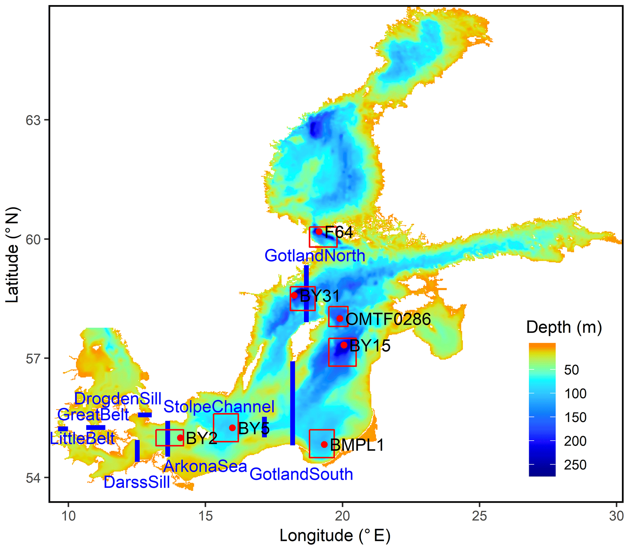
Figure 1 Model topography. Red dots: oceanographic stations. Red boxes: areas around these stations from which ICES observations were selected. Blue lines: transects across which transports were calculated.

The data for the individual stations are irregular in depth and time. To obtain time series for surface and bottom salinity, we select all data from the uppermost 20 m and from the depth range between 90 % and 100 % of the water depth at the station location, respectively. All measurements from the same day are averaged. Calculating annual or longer-term averages from the time series is not straightforward, since a seasonal sampling bias may occur. To correct for this, we follow the method proposed by Simpson (2014). We fit a generalized additive mixed model (GAMM) through the data, which explains them as a sum of a smooth decadal variation s_Longterm(t_i); a smooth seasonal signal s_Seasonal(τ_i), where τ_i denotes the sampling time within a year, ranging between 0 at 1 January and 1 at the end of 31 December; a constant offset S₀; and residuals ϵ_i, whose temporal autocorrelation is assumed to follow a continuous AR(1) model:

$$\begin{array}{}\text{(1)}& S_i=s_{\mathrm{Longterm}}\left(t_i\right)+s_{\mathrm{Seasonal}}\left({\mathit{\tau }}_i\right)+S_{\mathrm{0}}+{\mathit{ϵ}}_i.\end{array}$$

By investigating the autocorrelation of the normalized residuals, we confirm that the autocorrelation model is applicable. We use the function gamm from the R package mgcv (version 1.8-31) to fit the model by a restricted maximum likelihood approach. The functions s_Longterm and s_Seasonal are defined as penalized cubic (and cyclic cubic) regression splines. We allow 1 degree of freedom per decade for s_Longterm and 1 degree of freedom per month for s_Seasonal. By subtracting the climatological seasonal salinity signal from the observations, we obtain the deseasonalized salinities as

$$\begin{array}{}\text{(2)}& S_i^{\mathrm{corr}}=S_i-s_{\mathrm{Seasonal}}\left({\mathit{\tau }}_i\right).\end{array}$$

These are used to calculate annual and decadal means for surface and bottom salinity at each station.

2.1.2 HIRESAFF v2 atmospheric reconstruction

The second dataset is the HIRESAFF v2 atmospheric reconstruction for the period 1850–2008 (Schenk and Zorita, 2012). This is a reconstruction of past atmospheric states by the analogue method (AM), which reconstructs historical atmospheric states by choosing analogue situations from a reference period in the recent past, based on similarity in a constrained number of observed variables. This dataset has been successfully applied for model-based Baltic Sea reconstructions in the past. The basin-integrated BALTSEM model was applied by Gustafsson et al. (2012) and a 2 nautical mile (nmi) Rossby Centre Ocean mode (RCO) model was used by Meier et al. (2012, 2018b). These studies, however, had their focus on the reconstruction of marine biogeochemistry. Two different ocean models (Modular Ocean Model, MOM, and RCO, 3 and 2 nmi resolution, respectively) were used by Kniebusch et al. (2019) to investigate Baltic Sea temperature variability over the 1850–2008 period.

Our comparison of the wind speed statistics in the dataset with observed winds at a set of Swedish coastal stations (Höglund et al., 2009) revealed that strong wind speeds were occurring less frequently in the atmospheric reconstruction than in the observations. Before driving our model, we therefore corrected the wind speeds by the following piecewise linear formula:

$$\begin{array}{}\text{(3)}& u_{\mathrm{new}}=u_{\mathrm{old}}+u_{\mathrm{0}}\cdot min\left(u_{\mathrm{old}}/u_{\mathrm{1}},\mathrm{1}\right),\end{array}$$

where u₀=0.7 m s⁻¹ is the correction for strong winds and u₁=4.9 m s⁻¹ is the threshold velocity above which this correction is fully applied.

In addition to driving the ocean model, we also use the wind data, specifically the third power of the wind speed, as a proxy for wind energy input into the ocean, where part of it is transformed into turbulent kinetic energy. From the 10 m wind speeds u₁₀ and v₁₀ given in the atmospheric forcing dataset, we calculate the third power of the wind speed as $u^{\mathrm{3}}={\sqrt{u_{\mathrm{10}}^{\mathrm{2}}+v_{\mathrm{10}}^{\mathrm{2}}}}^{\mathrm{3}}$. We obtain a time series for each oceanographic station listed in Sect. 2.2 by averaging this value over the corresponding rectangle shown in Fig. 1, whose coordinates are given in Appendix A. The motivation to use the third power of the wind speed is that the wind work, i.e. the kinetic energy input by wind, scales with the third power of the wind (Elsberry and Garwood, 1978).

2.1.3 River runoff

The third dataset describes monthly river runoff, which we adopt from a previous model study (Meier et al., 2018a). Monthly river discharges were merged in time from different sources, i.e. reconstructions by Hansson et al. (2011) for 1850–1900, Cyberski et al. (2000) for 1901–1920, and Mikulski (1986) for 1921–1949; observations from the BALTEX Hydrological Data Center (BHDC) (Bergström and Carlsson, 1994) for 1950–2004; and hydrological model results Graham (1999) for 2005–2008. We choose the ArkonaSea transect (see Fig. 1) and aggregate the runoff of the Baltic Sea rivers eastward of the transect to obtain a cumulated runoff time series.

2.1.4 Baltic inflow reconstruction

The fourth dataset is a reconstruction of Baltic inflows by Mohrholz (2018). For 1426 barotropic inflow events of different strength between 1887 and 2018, the inflowing mass of salt (in Gt) across Darss and Drogden Sill was reconstructed based on sea level and salinity from the Belt Sea and the Sound and river discharge. These events are differentiated into large inflows (category DS5, indicating that a threshold salinity was exceeded for at least 5 consecutive days at Darss Sill) and smaller ones. For each of these categories, we obtain three annual time series: (a) total mass of imported salt, (b) number of events during the year, and (c) average strength of the events during the year (salt mass imported during individual event). For those years where no events occurred, we use linear interpolation in time series (c) to fill the gaps. This may lead to an overestimation of inflow strength when years with strong inflows are followed by years without inflow activity, but we need to generate a complete time series to apply the wavelet analysis method.

2.1.5 Climate indices

Finally, the fifth dataset consists of the climate indices AMO and NAO. The NAO is a dimensionless index traditionally describing the anomaly of the surface pressure difference between the Azores and Iceland. We use a dataset based on the pressure difference between Gibraltar and Iceland (Jones et al., 1998) extending backwards until 1821. The AMO index describes a sea surface temperature (SST) anomaly of the Northern Atlantic. We use an AMO index calculated from the SST in the latitude–longitude range of 25–60^∘ N and 7–75^∘ W minus a regression on the global mean temperature as described by van Oldenborgh et al. (2009), based on the Hadley Center SST dataset HadSST 3.1.1.0 (Kennedy et al., 2011a, b). Both datasets were downloaded from the Royal Netherlands Meteorological Institute (KNMI) climate explorer dataset collection (KNMI, 2019).

2.2 Model simulation

We use two models in the study: a 3D hydrodynamic model and a box model. This section is about the 3D model; the box model is described in Sect. 2.5.

Salinities and salt transports for the period 1850–2008 are obtained from a hindcast simulation with the General Estuarine Transport Model (GETM, https://getm.eu/, last access: 18 August 2020). This hydrodynamic model solves the hydrostatic Boussinesq equations on a regular latitude–longitude grid with approximately 1 nmi horizontal resolution. The model topography (see Fig. 1) is based on the iowtopo bathymetry (Seifert et al., 2001) but has been smoothed to reduce numerical mixing, since large numerical mixing causes too quick a degradation of the halocline during stagnation periods. Manual corrections were applied in the Danish Straits where the grid resolution only allows a rough representation of the topographic features. In the vertical, the model has 50 layers with vertically adaptive coordinates (Gräwe et al., 2019). Compared to traditional z or σ coordinates, these allow a higher resolution in the proximity of pronounced density gradients, which reduces numerical mixing. More details on the model setup can be found in Appendix C.

Our model was integrated for 159 years from 1850 to 2008. Atmospheric forcing conditions are prescribed from the HIRESAFF v2 dataset (Schenk and Zorita, 2012) which spans this period. Reconstructed river runoff and open boundary conditions for the simulation period were adopted from a previous model study (Meier et al., 2018a).

For the comparison of time series between model and observations, we use the classical measure of explained variance, defined as (e.g. Good and Fletcher, 1981)

$$\begin{array}{}\text{(4)}& {\mathit{\rho }}^{\mathrm{2}}={\displaystyle \frac{{\mathit{\sigma }}_{\mathrm{obs}}^{\mathrm{2}}-{\mathit{\sigma }}_{\mathrm{res}}^{\mathrm{2}}}{{\mathit{\sigma }}_{\mathrm{obs}}^{\mathrm{2}}}}.\end{array}$$

Here, ${\mathit{\sigma }}_{\mathrm{obs}}^{\mathrm{2}}$ is the variance in the observations and ${\mathit{\sigma }}_{\mathrm{res}}^{\mathrm{2}}$ is the variance in the residuals, i.e. the difference between observations and model. The explained variance is 1 if, and only if, the residuals vanish. It is typically between 0 and 1 but can also become negative if the deviations between model and observations show a larger variance than the observations themselves.

2.3 Salinity-discriminated transports

Salt and volume transports as well as mean salinities were stored in daily resolution at selected transects for each grid point and vertical layer. From these data, transports per salinity interval were calculated, following the total exchange framework (TEF) analysis framework (Walin, 1977, 1982; MacCready, 2011; Burchard et al., 2018) in order to discriminate between import and export of salt. The procedure is as follows. In a first step, we define salinity limits every 0.025 g kg⁻¹ between 0 and 36 g kg⁻¹. For each of these salinity limits, we calculate the sum of transports over all grid cells and vertical layers with a mean salinity above this limit:

$$\begin{array}{}\text{(5)}& T_{S^{*},t}=\sum _i\sum _k{T}_{i,k,t}\cdot \mathit{\theta }\left(S_{i,k,t}-S^{*}\right),\end{array}$$

where $T_{i,k,t}$ denotes the salt transport across the transect in grid cell i and layer k during time step t; $S_{i,k,t}$ denotes the average salinity in this grid cell, layer, and time step; S^* is the salinity limit above which the transport is measured; and θ denotes the Heaviside step function, θ(x)=1 for x>0 and θ(x)=0 otherwise. It should be noted that while the total transports across the transect are exactly quantified by the model, their attribution to the salinity bins contains some uncertainty depending on the model output frequency. The transports are counted as positive if they are directed into the Baltic Sea.

Let us consider the time-averaged salinity-discriminated transports $T_{S^{*}}$ as a function of S^*. These have a typical shape as shown in Fig. 2. They are 0 at high salinities, show a maximum value $T_{\widehat{S}}$ at a salinity of $\widehat{S}$, which depends on the cross section, and then decrease again as salinity approaches 0.¹ This reflects the fact that net inflow occurs on average for salinities above $\widehat{S}$ (near the bottom), while net outflow occurs at lower salinities (near the surface). The value $\widehat{S}$ denotes the salinity class where inflow and outflow compensate for each other. We can then derive salinity quantiles of the net import and net export as shown in Fig. 2. The value $S_{\mathrm{in}}^{p\mathit{\%}}$ shall define the salinity above which p % of the net inflow occurs; it can be determined from the salt transports by

$$\begin{array}{}\text{(6)}& T_{S_{\mathrm{in}}^{p\mathit{\%}}}={\displaystyle \frac{p}{\mathrm{100}}}\cdot T_{\widehat{S}}\mathrm{and}{S}_{\mathrm{in}}^{p\mathit{\%}}\ge \widehat{S}.\end{array}$$

We determine two time series for net imports across each transect.

$$\begin{array}{}\text{(7)}& T_{\mathrm{highsal},t}=T_{S_{\mathrm{in}}^{\mathrm{50}\mathit{\%}},t}\end{array}$$

denotes the net import in the high-salinity range, while

$$\begin{array}{}\text{(8)}& T_{\widehat{S},t}=T_{S_{\mathrm{in}}^{\mathrm{100}\mathit{\%}},t}\end{array}$$

denotes the net import at all salinities above $\widehat{S}$. The import at low salinities, T_lowsal,t, is the difference between the two.

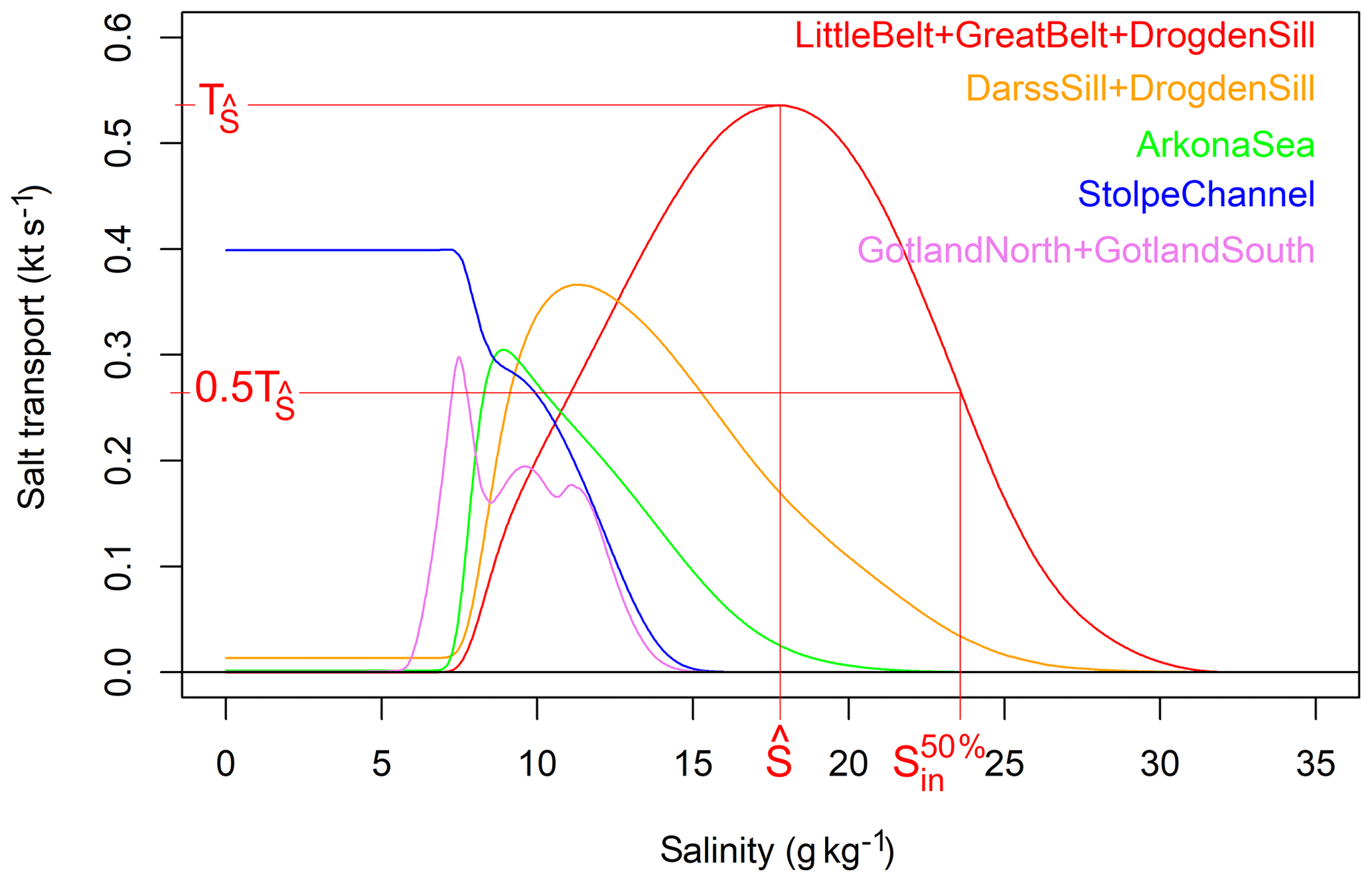
Figure 2 Net salt transports into the Baltic Sea above a specific salinity level, temporal average across the simulation period 1850–2008. Horizontal and vertical lines visualize how the threshold salinity $S_{\mathrm{in}}^{\mathrm{50}\mathit{\%}}$ for discriminating between the import of high-salinity and low-salinity water is determined.

2.4 Wavelet analysis

Summarizing the above sections, we obtained the following collection of time series, which start in the 19th century with at least annual resolution:

• modelled surface or bottom salinity for each oceanographic station (from 3D model)

• third power of the wind speed as a proxy for wind work for each oceanographic station (Schenk and Zorita, 2012)

• three time series for net salt transports into the Baltic Sea (T_highsal,t, T_lowsal,t, $T_{\widehat{S},t}$) for each transect (from 3D model)

• salt import, inflow frequency, and strength reconstructed by Mohrholz (2018) for Darss Sill

• river runoff into the Baltic Sea, inside the ArkonaSea transect (Meier et al., 2018a)

• two prominent climate indices for Europe, NAO, and AMO (KNMI, 2019).

To find out at which timescales the variations in the time series occur, we investigate them with the wavelet analysis method. To explore the correlations between different time series in specific frequency bands, we apply wavelet coherence analysis.

Wavelet analysis is a generalization of Fourier analysis and also aims at separating signals in different frequency ranges. In Fourier transform, we use the highest possible frequency resolution, which is determined by the step width of the time series under investigation. The amplitude for each frequency range is then calculated by a convolution of the time series with an infinite harmonic function. The price for the high frequency resolution is the loss of all temporal information, which is then only stored in the Fourier phases. In a wavelet transform, we calculate the convolution with time-limited functions. The Morlet wavelet we use has the shape

$$\begin{array}{}\text{(9)}& \mathit{\varphi }(a,t)={\displaystyle \frac{\sqrt{\mathrm{2}}}{\sqrt{\mathit{\pi }}a}}\exp \left(-i{\mathit{\omega }}_{\mathrm{0}}{\displaystyle \frac{t}{a}}\right)\exp \left(-{\displaystyle \frac{t^{\mathrm{2}}}{\mathrm{2}{a}^{\mathrm{2}}}}\right),\end{array}$$

where a is the wavelet width (in time units) and ω₀ is a dimensionless shape parameter which controls whether the resolution of the wavelet analysis is higher in the frequency range or the temporal range. The wavelet transform is calculated as

$$\begin{array}{}\text{(10)}& W(a,t)=\underset{\mathit{\tau }=-\mathrm{\infty }}{\overset{\mathrm{\infty }}{\int }}\mathrm{d}\mathit{\tau }x\left(\mathit{\tau }\right)\mathit{\varphi }(a,t-\mathit{\tau }).\end{array}$$

For analysing whether two time series x(t) and y(t) share energy in a specific frequency band at the same time, we calculate common wavelet power (CWP) and wavelet coherence. Common wavelet power is just the product of the wavelet amplitudes:

$$\begin{array}{}\text{(11)}& \mathrm{CWP}(a,t)=\left|W_x(a,t)W_y(a,t)\right|.\end{array}$$

If we regard x(t) as the time series to be explained and y(t) as a possible driver of it, we normalize the latter time series by dividing through its standard deviation such that the common wavelet power has the same unit as the original time series x(t).

Wavelet coherence is a measure which determines how stable the relative phase between two time series around a specific point in the time–frequency plane is. As pointed out by Maraun and Kurths (2004), an interrelation between two time series should not only be identified by strong CWP but also by a stability in the phase difference. Wavelet coherence is calculated as

$$\begin{array}{}\text{(12)}& {\mathit{\rho }}_{xy}(a,t)={\displaystyle \frac{<W_x(a^{\prime },t^{\prime })W_y*(a^{\prime },t^{\prime })>}{\sqrt{<\left|W_x\right(a^{\prime },t^{\prime }){|}^{\mathrm{2}}><|W_y(a^{\prime },t^{\prime }){|}^{\mathrm{2}}>}}}\end{array}$$

(Aguiar-Conraria and Soares, 2011), where the pointed brackets mean a smoothing over a time and frequency range around the central point (a,t). In the simplest case this can be a box average over a time and frequency interval. In the case of the relative phase being equal throughout this range, it can be factored out from the averaging operator in the numerator, so ρ_xy has a magnitude of 1 then. If, in contrast, the relative phase varies strongly across the averaging interval, the magnitude of ρ_xy will be close to 0.

Details on the wavelet calculations can be found in Appendix D. To assess whether the correlations identified with the wavelet methods are significant, we compare the magnitudes of W(a,t) and CWP(a,t) with those of surrogate time series which were created by block-shuffling complete years in the individual time series. Where the magnitudes exceed those of 95 % of the surrogate time series, we regard them as significant.

2.5 Salt budget calculations to estimate the direct dilution effect

A budget method is used with the aim to discriminate between salinity changes due to direct dilution by river water and reduced salt import into the Baltic Sea. We separate the water volume of the Baltic Sea inside the ArkonaSea transect by an isohaline at a constant salinity S_isohaline. We then calculate time series for the volume V and salt mass s both above and below the isohaline. The volume and salt fluxes into and out of the compartments are denoted in Fig. 3.

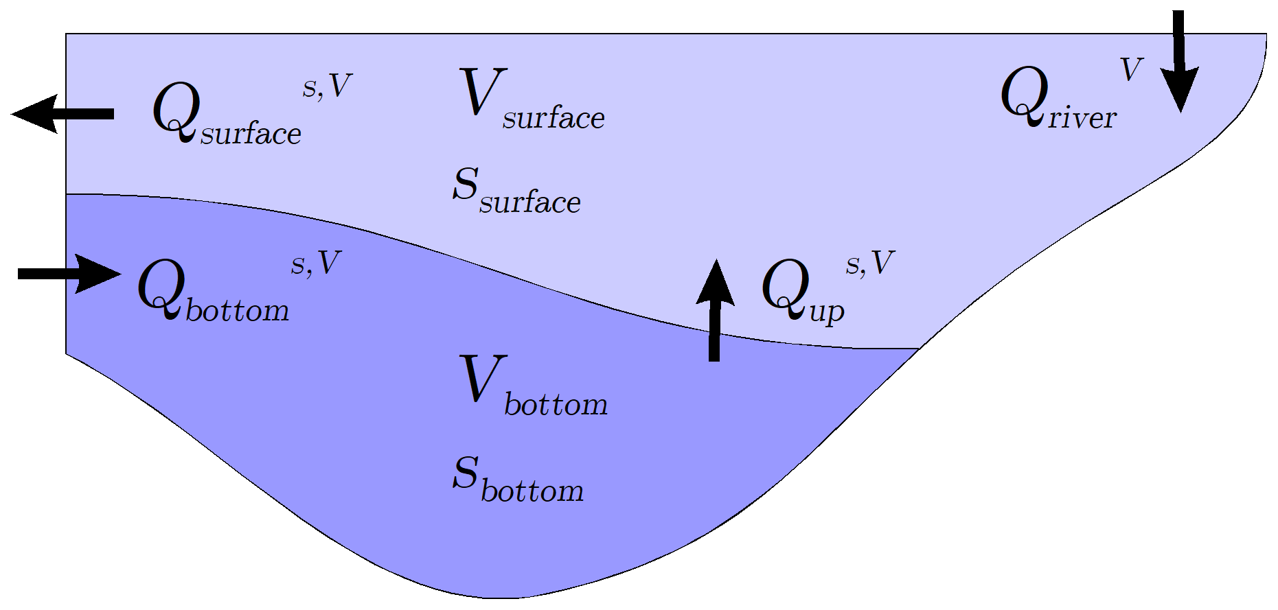
Figure 3 Schematic view of salt and volume fluxes in and out of two compartments, separated by an isohaline. The volumes V and salt masses s inside these compartments change over time.

From the volume and salt budget of the water body below the isohaline, we can calculate the upward transport of volume and salt into the overlying water:

$$\begin{array}{}\text{(13)}& {\displaystyle }{Q}_{\mathrm{up}}^s& {\displaystyle }=Q_{\mathrm{bottom}}^s-{\displaystyle \frac{d}{\mathrm{d}t}}{s}_{\mathrm{bottom}},\text{(14)}& {\displaystyle }{Q}_{\mathrm{up}}^V& {\displaystyle }=Q_{\mathrm{bottom}}^V-{\displaystyle \frac{d}{\mathrm{d}t}}{V}_{\mathrm{bottom}}.\end{array}$$

In a similar way, we can calculate the export across the transect in the overlying water:

$$\begin{array}{}\text{(15)}& {\displaystyle }{Q}_{\mathrm{surface}}^s& {\displaystyle }=Q_{\mathrm{up}}^s-{\displaystyle \frac{d}{\mathrm{d}t}}{s}_{\mathrm{surface}},\text{(16)}& {\displaystyle }{Q}_{\mathrm{surface}}^V& {\displaystyle }=Q_{\mathrm{up}}^V+Q_{\mathrm{river}}^V-{\displaystyle \frac{d}{\mathrm{d}t}}{V}_{\mathrm{surface}}.\end{array}$$

We assume that the surface salt export is approximately determined from volume export and the surface concentration of salt: s_surface∕V_surface. We derive an approximation by

$$\begin{array}{}\text{(17)}& {\stackrel{\mathrm{̃}}{Q}}_{\mathrm{surface}}^s=\mathit{\alpha }{\displaystyle \frac{Q_{\mathrm{surface}}^V{s}_{\mathrm{surface}}}{V_{\mathrm{surface}}}},\end{array}$$

where the parameter α accounts for horizontal inhomogeneity in the salinity. It is determined by a least-squares fit of ${\stackrel{\mathrm{̃}}{Q}}_{\mathrm{surface}}^s$ to $Q_{\mathrm{surface}}^s$; we obtain a value of α=1.17. (The error by the simplification of choosing a constant α will be discussed a posteriori.) If we insert the approximation (17) into (15), we obtain a differential equation for s_surface as follows:

$$\begin{array}{}\text{(18)}& {\displaystyle \frac{d}{\mathrm{d}t}}{s}_{\mathrm{surface}}=Q_{\mathrm{up}}^s-\mathit{\alpha }{\displaystyle \frac{Q_{\mathrm{surface}}^V{s}_{\mathrm{surface}}}{V_{\mathrm{surface}}}}.\end{array}$$

Here we can see how a direct dilution effect may affect the salinity. A higher river runoff enhances the outflow volume $Q_{\mathrm{surface}}^V$ and leads to a sinking salinity. The solution of the differential equation reads

$$\begin{array}{}\text{(19)}& s_{\mathrm{surface}}=A\left(t\right)\left(\underset{t_{\mathrm{0}}}{\overset{t}{\int }}{\displaystyle \frac{Q_{\mathrm{up}}^s}{A\left(t^{\prime }\right)}}\mathrm{d}{t}^{\prime }+C_{\mathrm{1}}\right),\end{array}$$

with

$$\begin{array}{}\text{(20)}& A\left(t\right)=\exp \left(-\underset{t_{\mathrm{0}}}{\overset{t}{\int }}\mathit{\alpha }{\displaystyle \frac{Q_{\mathrm{surface}}^V}{V_{\mathrm{surface}}}}\mathrm{d}{t}^{\prime }\right).\end{array}$$

We prescribe the initial salt content, which fixes the integration constant C₁ at

$$\begin{array}{}\text{(21)}& C_{\mathrm{1}}=s_{\mathrm{surface}}\left(t_{\mathrm{0}}\right).\end{array}$$

To calculate the solution of the differential equation, we use annual means of the fluxes across the ArkonaSea transect and of the volumes and salt contents above and below the halocline. The solution of this simplified salinity estimator is compared to the results of the full model to prove the applicability of the method. After this has been shown, we solve the equation again for a temporally constant river runoff but keeping the salt and volume fluxes through the halocline constant. The difference between the two salinity time series then measures the direct dilution effect.

3 Numerical model validation

3.1 Surface and bottom salinity at selected stations

The surface and bottom salinities at the selected stations shown in Fig. 1 are compared to ICES observations from rectangles around the station location. Figure 4 shows this comparison for annual and 11-year running means of surface and bottom salinity. The comparison shows that a substantial part of the interdecadal variability at most stations is reproduced by the model. Modelled salinities, however, show a positive bias which increases with latitude.

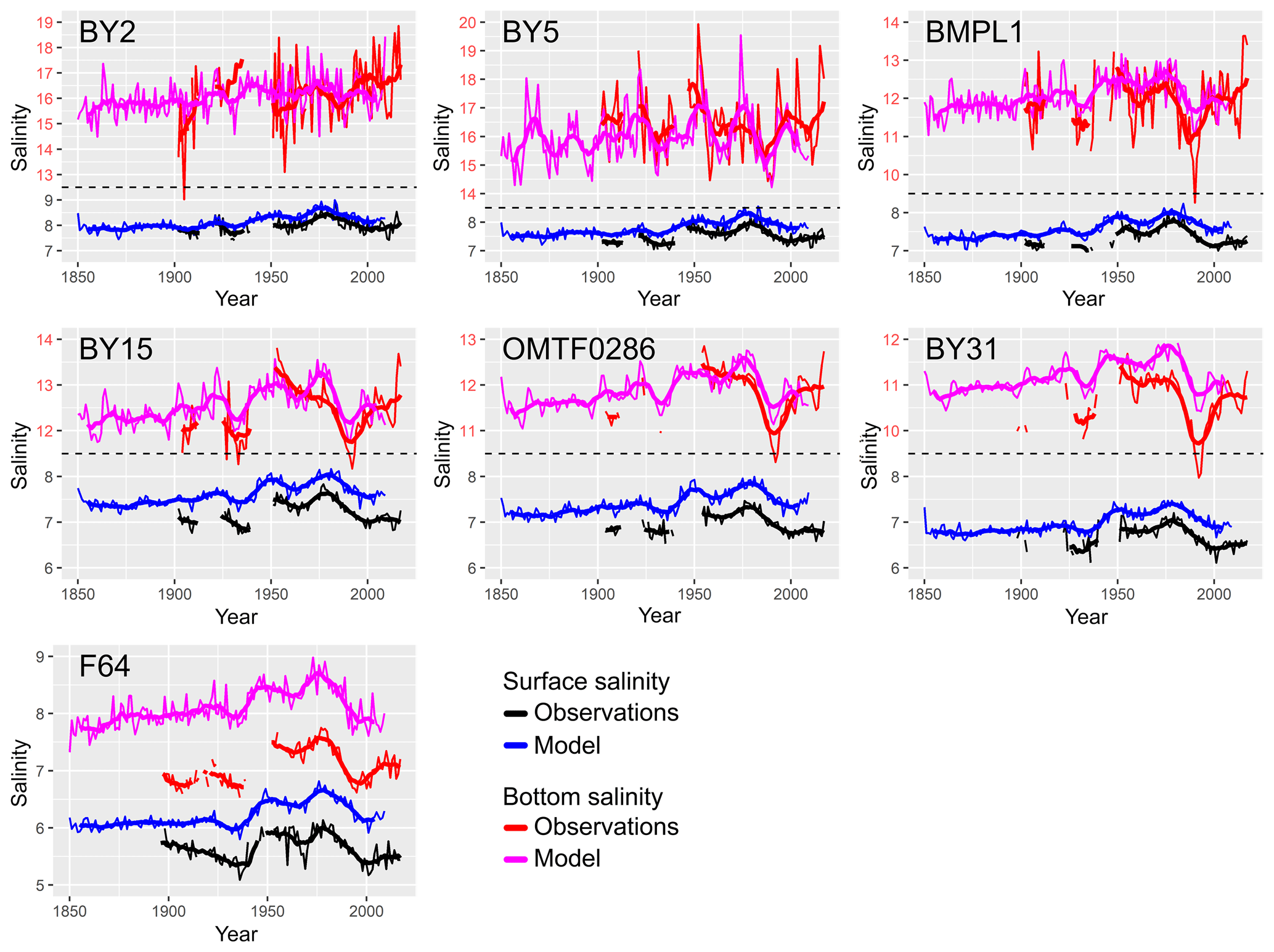
Figure 4 Surface and bottom salinity at selected oceanographic stations from observations and model. Thin lines: annual averages. Thick lines: 11-year running mean. Data are corrected for seasonal observation bias. Running mean is shown where at least 6 years of data were available. Dashed lines and red axis annotations indicate a broken salinity axis for better visibility.

Table 1 Basic statistics for fit between model and observations with respect to surface and bottom salinities.

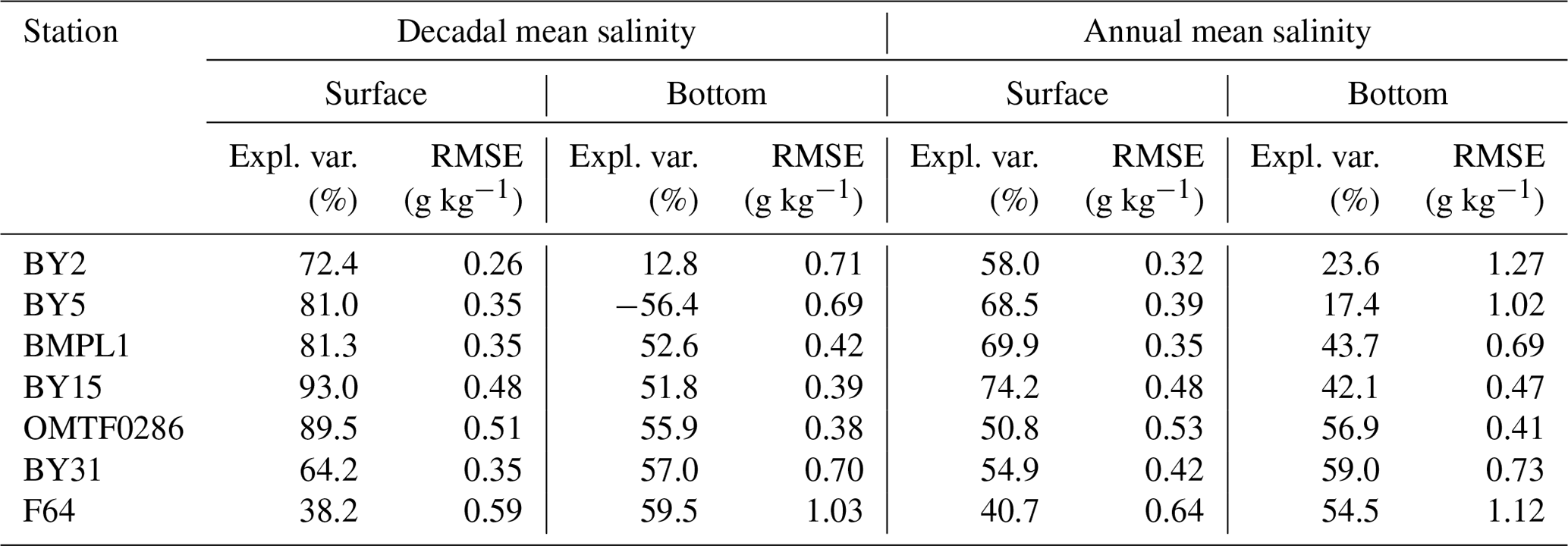
Table 1 shows the explained variance and the root-mean squared error between model and observations. The model captures the variability in surface salinities better than that of bottom salinities. The decadal variations in surface salinity in particular are well captured by the model: more than 80 % of the variance can be explained by the model in the Eastern Gotland Basin and in the Bornholm Basin. For the bottom salinities, the model can explain about half of the variability in the central Baltic, both in the annual and the decadal means. In the western Baltic, however, a smaller fraction of the variance is explained, and for the decadal mean at Bornholm Deep (BY5) the differences between model and observations even show a larger variance than the observations themselves. We therefore focus on station BY15 when we consider modelled bottom salinities.

The question of why the bottom salinities can match better in the central Baltic compared to the entrance area is discussed in Appendix E.

3.2 Transports across the sills

Volume transport across the DrogdenSill transect was compared to a simple linear model which is based on the sea levels in Klagshamn and Viken: z_K and z_V. From these, the transport can be approximated, following Håkansson et al. (1993), by

$$\begin{array}{}\text{(22)}& T_{\mathrm{Vol}}=Q\sqrt{\mathrm{\Delta }{z}^{\prime }}{\displaystyle \frac{\mathrm{\Delta }{z}^{\prime }}{\left|\mathrm{\Delta }{z}^{\prime }\right|}},\end{array}$$

where

$$\begin{array}{}\text{(23)}& \mathrm{\Delta }{z}^{\prime }=z_{\mathrm{K}}-z_{\mathrm{V}}\left(\mathrm{1}+\mathrm{0.16}\mathit{\theta }\left(z_{\mathrm{K}}-z_{\mathrm{V}}\right)\right)\end{array}$$

is the corrected sea level difference between the two stations, θ denotes the Heaviside step function, and Q=74770 m^5∕2 s⁻¹ is an empirical constant. Hourly tide gauge data were downloaded from the GESLA (Global Extreme Sea Level Analysis) portal (https://gesla.org/, last access: 18 August 2020), and daily volume transports were calculated from them. A comparison to the results of the numerical model showed that the model transports had a 24 % higher standard deviation, but the correlation coefficient between both time series is R=0.766 (R²=58.6 %). For the DarssSill transect, we used observations from an acoustic Doppler current profiler (ADCP) at a permanent observation station (54.7^∘ N, 12.7^∘ E) and directly compared them to our model velocities at the nearest grid point. Observations were taken from the database of the Leibniz Institute for Baltic Sea Research Warnemünde (https://odin2.io-warnemuende.de, last access: 18 August 2020), and daily-mean eastward velocities at 3 and 17 m depth were compared between model and measurements for the period 1995–2008. Figure 5 shows a visual comparison for the first few years. It can be seen that the time series compare reasonably well in most situations, while the model overestimates near-surface peak velocities during outflow situations. Correlating observed and modelled velocities gives a coefficient of determination of R²=43.5 % and 40.5 % of the variance at 3 and 17 m depth, respectively.

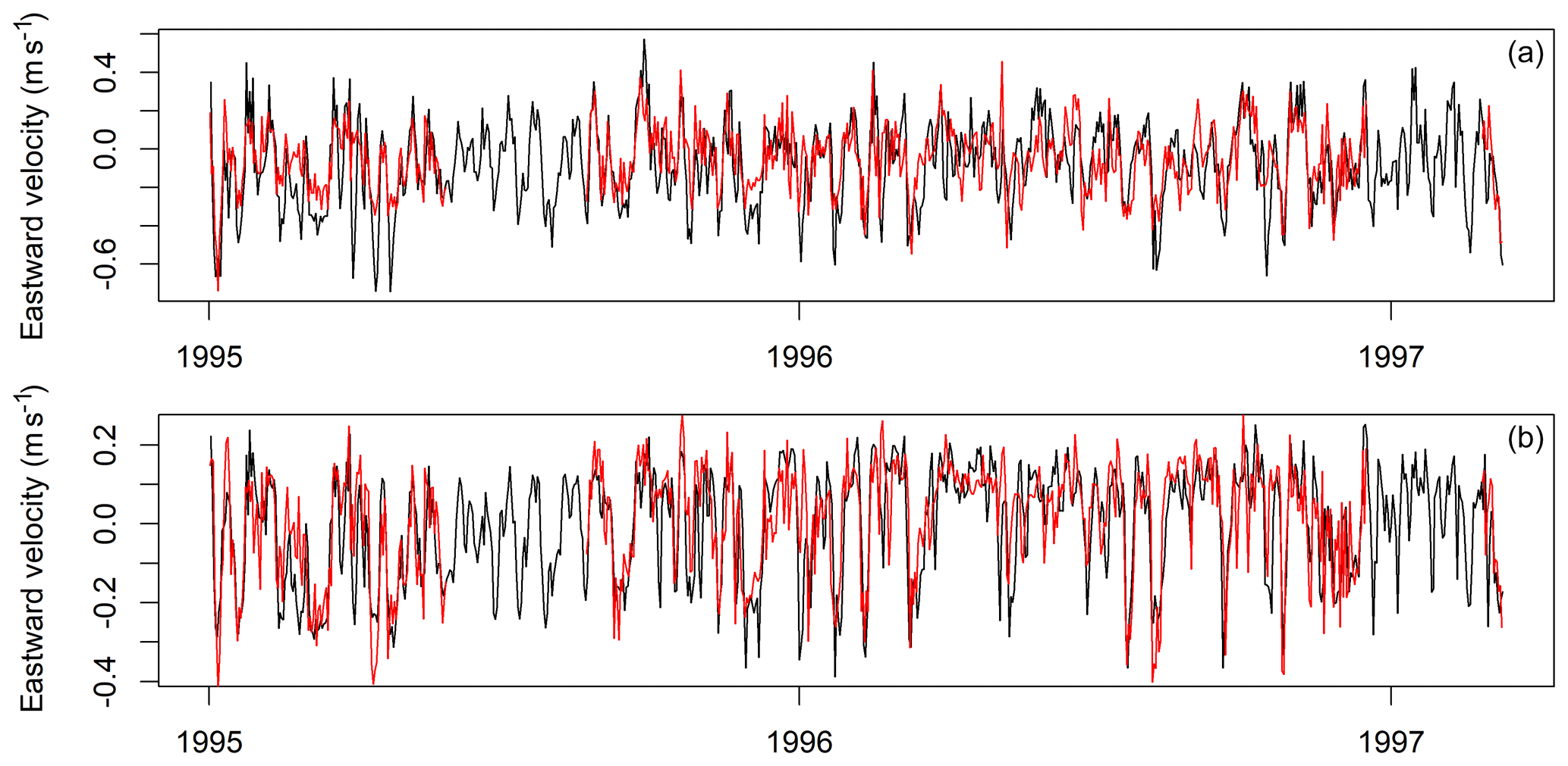
Figure 5 Eastward velocity at station Darss Sill (54.7^∘ N, 12.7^∘ E): (a) at 3 m depth; (b) at 17 m depth. Black line: model results. Red line: ADCP observations.

4 Results of wavelet analysis

4.1 Interdecadal changes in salinity

Wavelet analysis of both surface and bottom salinities highlighted a signal with a 30-year periodicity; see Figs. 6 and 7. It becomes prominent in the first half of the 20th century in the model. Since the observations only start in the end of the 19th century, it is impossible to decide whether the signal starts earlier in the observations. For the surface salinities, the signal is significant for all of the considered stations both in the model and the observations. For the bottom salinities, the 30-year signal is present for all stations except for those in the Arkona and Bornholm Sea (stations BY2 and BY5) where it is missing or shifted in frequency. The signal indicates a fluctuation with an amplitude of 0.2 g kg⁻¹ (or 0.4 g kg⁻¹ peak to peak) in the surface salinity. For the bottom salinities, the strength of the signal varies between 0.5 g kg⁻¹ in the Gdánsk Deep (Station BMPL1) and 0.2 g kg⁻¹ at the northernmost station F64. The model slightly underestimates this long-term signal. At some stations, additional significant variability exists at a periodicity of 10 years; however, this signal is episodic.

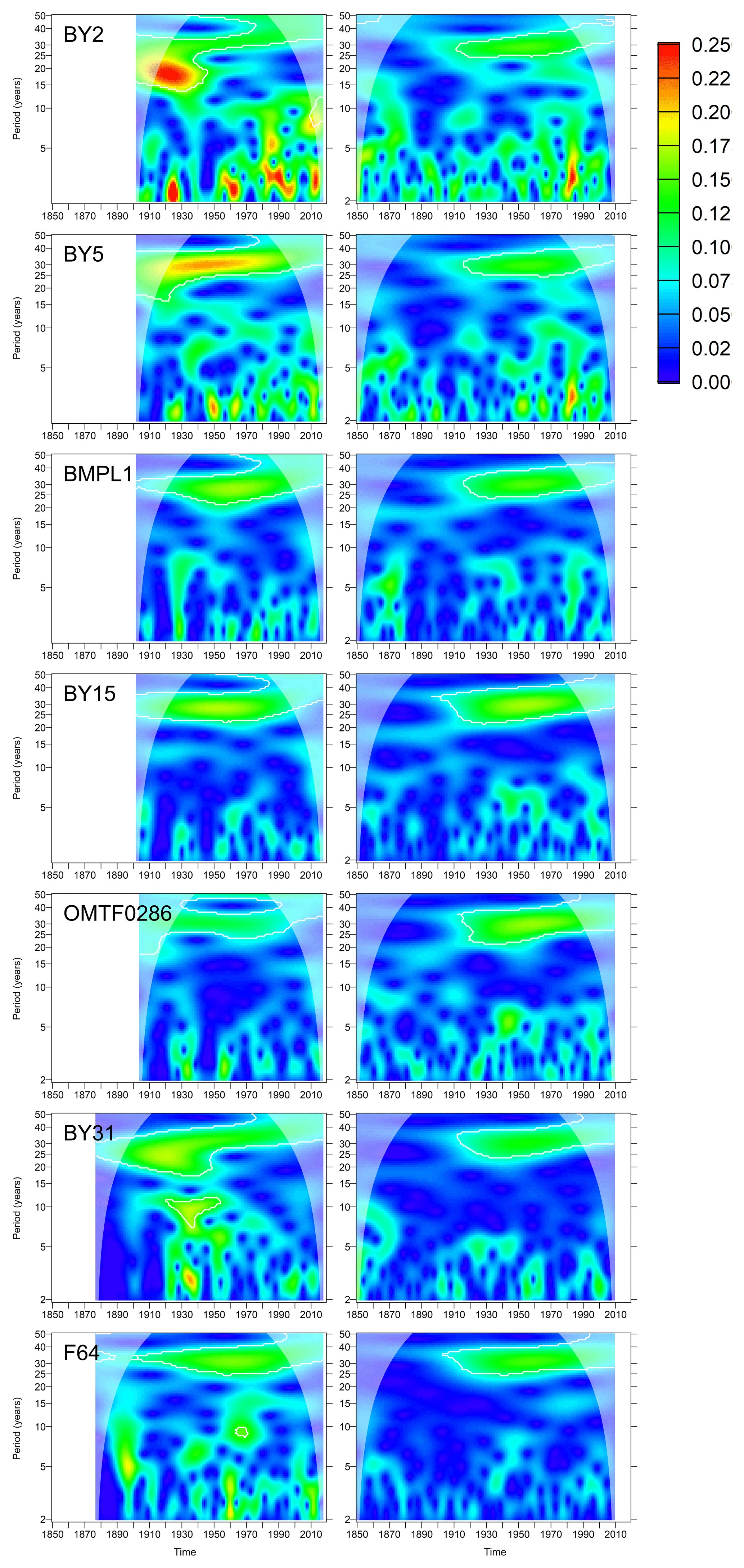
Figure 6 Wavelet amplitudes of surface salinities at selected oceanographic stations (g kg⁻¹). Left column: observations; right column: model results. White contours denote significant amplitudes at the 95 % confidence level compared to surrogate data randomized by shuffling the years.

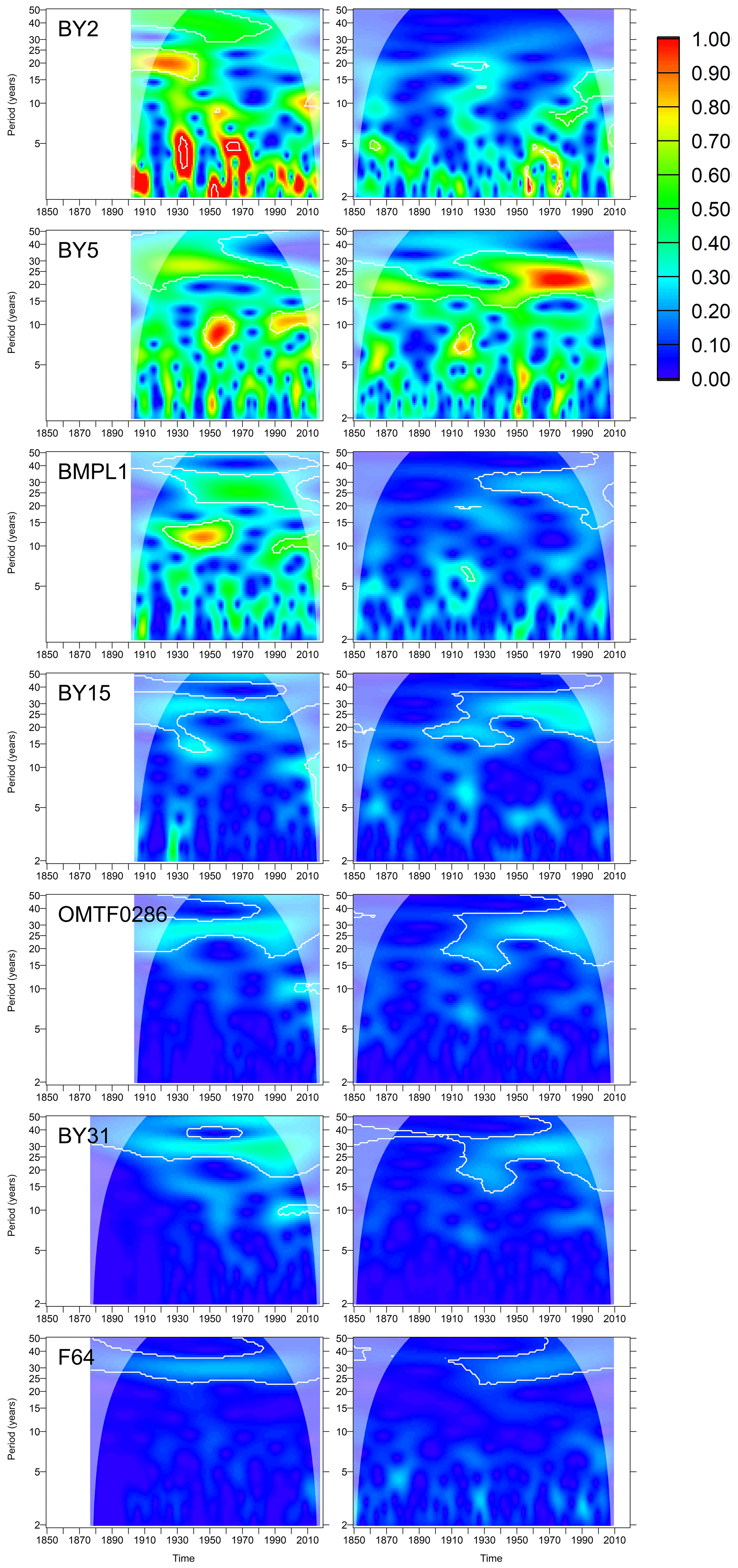
Figure 7 Wavelet amplitudes of bottom salinities at selected oceanographic stations (g kg⁻¹). Left column: observations; right column: model results. White contours denote significant amplitudes at the 95 % confidence level compared to surrogate data randomized by shuffling the years.

4.2 Relation to large-scale climate indices

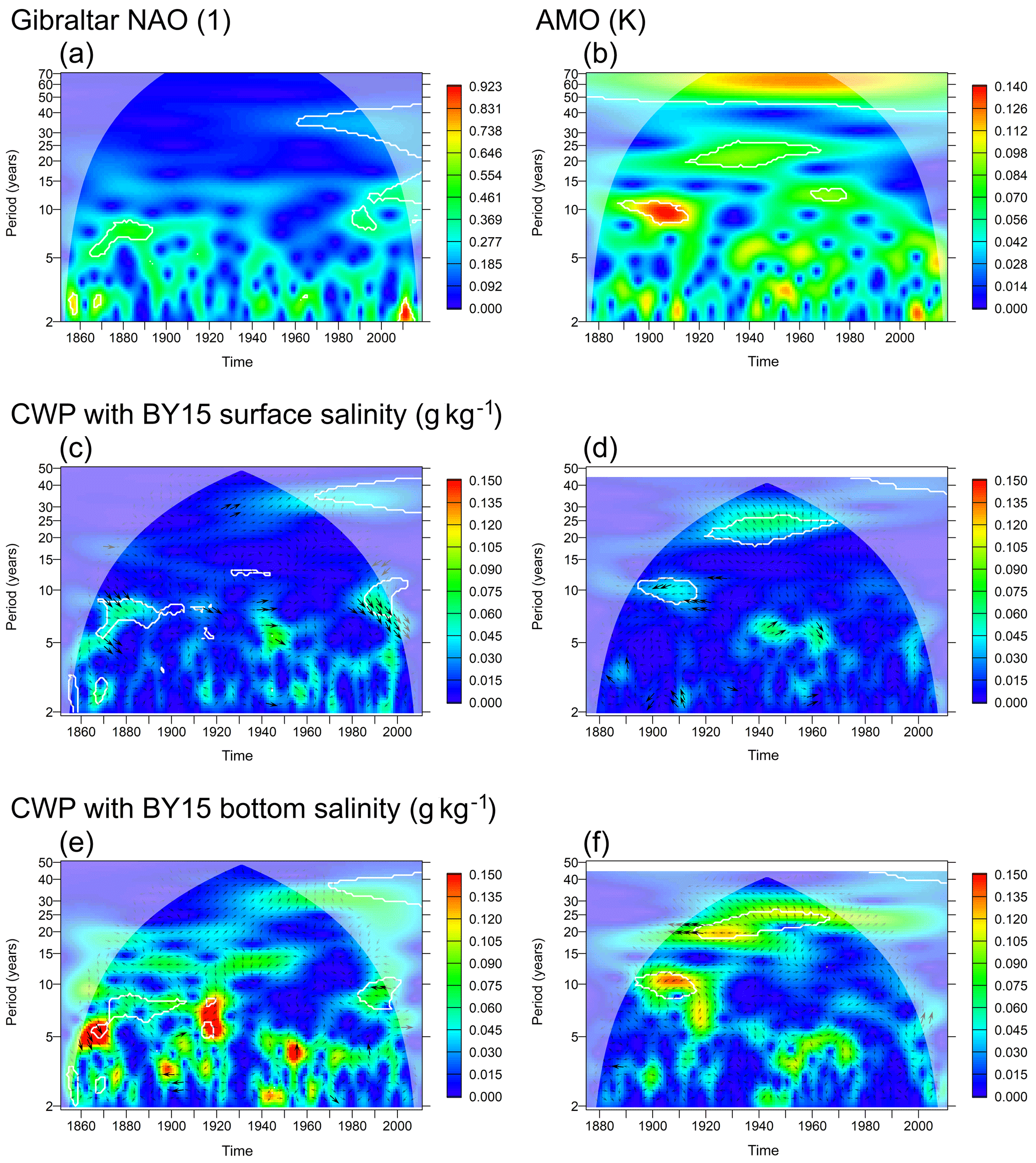
Figure 8 (a, b) Wavelet amplitudes (WAs) of NAO (Gibraltar–Iceland) and AMO index. (c–f) Common wavelet power (CWP) between modelled surface and bottom salinities at station BY15 and the normalized climate indices. White contours indicate that the WA or CWP is significant at the 95 % confidence level with respect to a random shuffling of the annual values of the climate index. Arrows indicate relative phase: →: in phase; ↓: climate index leading salinity by 90^∘. Thick arrows indicate phase stability (wavelet coherence > 0.95).

The wavelet decomposition of the NAO and AMO signal (Fig. 8a, b) shows that none of these indices shows the same pattern in the 30-year frequency band as the salinities. In the NAO signal, we find significant energy in this frequency band but only since the 1960s. In the AMO signal, a 60-year period is pronounced. We also find significant energy (with respect to white noise) in the band around 20–25 years, that is, at the higher range of the frequencies we observe in the salinity time series. This signal is, however, limited in time and no longer significant after the 1970s. To see whether the large-scale climate patterns described by the indices may explain the decadal variability in the salinity signal, we calculate common wavelet power between the modelled salinities at station BY15 and the normalized climate indices (Fig. 8, bottom rows). We find common wavelet power between NAO and the surface or bottom salinity in the range of 0.05 to 0.1 g kg⁻¹ around the 30-year frequency band, however, only from 1940 on and not statistically significant. Here, the NAO slightly lags behind the salinity signal with a wavelet coherence below 0.95. Stronger wavelet coherence is found in the frequency band between 5 and 10 years for the periods 1860–1880 and 1980–2000, where the NAO slightly leads surface salinity at station BY15. Alternative NAO indices were also investigated (Azores–Iceland annual and winter NAO), and no clear correspondence to the 30-year salinity signal was found either (not shown).

For the AMO, we find significant common wavelet power in the 20–25-year band. The phase relation between the signals is, however, changing. For the decade 1910–1920, we find wavelet coherence above 0.95 when AMO and bottom salinity are in anti-phase, however, at a period around 20 years. Later in the 20th century, the relative phase changes in the frequency band between 25 and 30 years, with the negative AMO then slightly leading the salinities in the 1920s to 1940s and later strongly leading it in the 1980s. This holds true for both surface and bottom salinities.

4.3 Processes related to interdecadal salinity changes

4.3.1 River runoff

The total river runoff eastward of the ArkonaSea transect (Fig. 1) has been calculated from the model forcing. Its wavelet decomposition is shown in Fig. 9. We find significant wavelet power from 1910 on in the 30-year frequency band, the oscillations inside a 30-year cycle amount to ±6 % of the mean runoff for the considered period. There is also significant common wavelet power in this frequency range, the CWP with bottom salinity being larger than that with surface salinity. The relative phase is stable (wavelet coherence mostly above 0.95) wherever common energy exists. In the 30-year frequency band, we find a 90^∘ phase shift (7.5-year lag, slightly less for bottom salinity) between the time series, with negative runoff anomalies leading high salinities. For surface salinities, this relation is stable over the entire 20th century; in the bottom salinity the lag reduces towards the end of the century. For the bottom salinities, we find similar phase relations also in the frequency bands between 3 and 15 years, with low runoff always occurring before high salinities, however, with a differing lag time (0.25–1.5 years). Using observed instead of modelled salinities gives the same results (not shown).

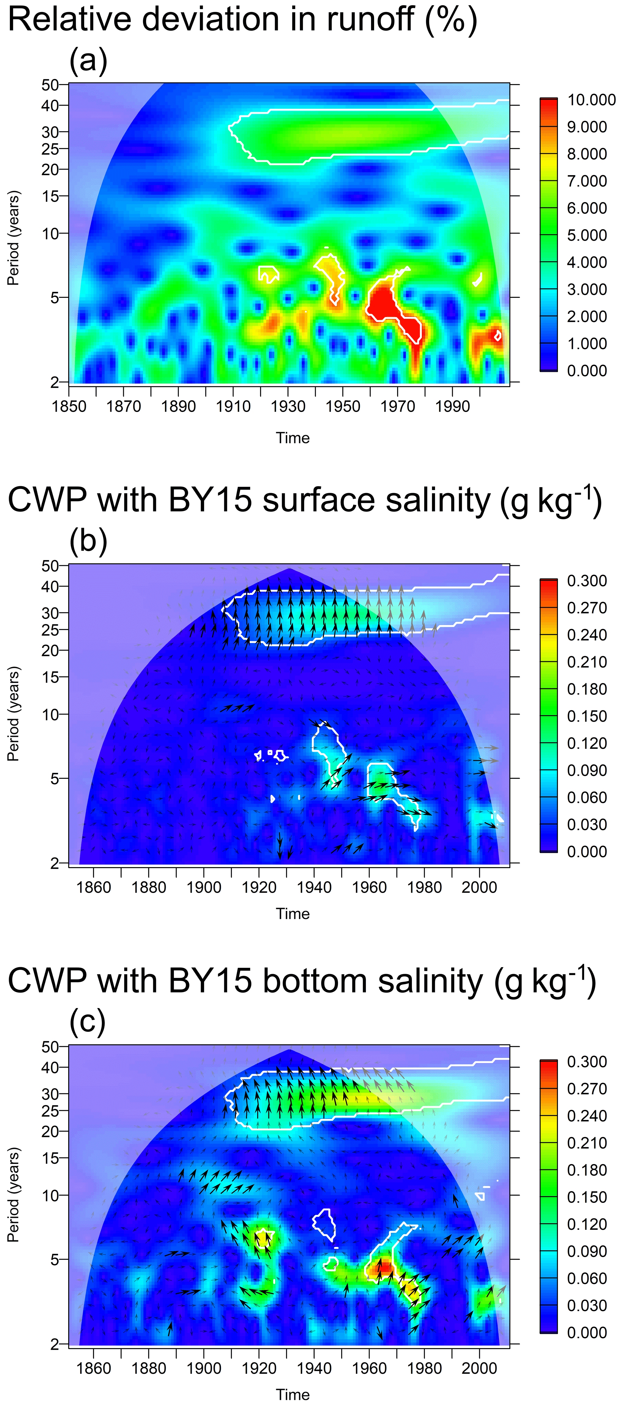
Figure 9 (a) Wavelet amplitude of the relative deviation in runoff of all model rivers inside the ArkonaSea transect; see Fig. 1. (b) Common wavelet power between modelled surface salinity at station BY15 (Eastern Gotland Basin, g kg⁻¹) and normalized runoff; note that the scale is doubled from Fig. 8. (c) The same for bottom salinity. White contours indicate that the WA or CWP is significant at the 95 % confidence level with respect to a random shuffling of the annual means of the runoff. Arrows indicate relative phase: →: high runoff and salinity in phase; ↑: low runoff leading salinity by 90^∘. Thick arrows indicate phase stability (wavelet coherence > 0.95).

4.3.2 Frequency versus strength of inflow events

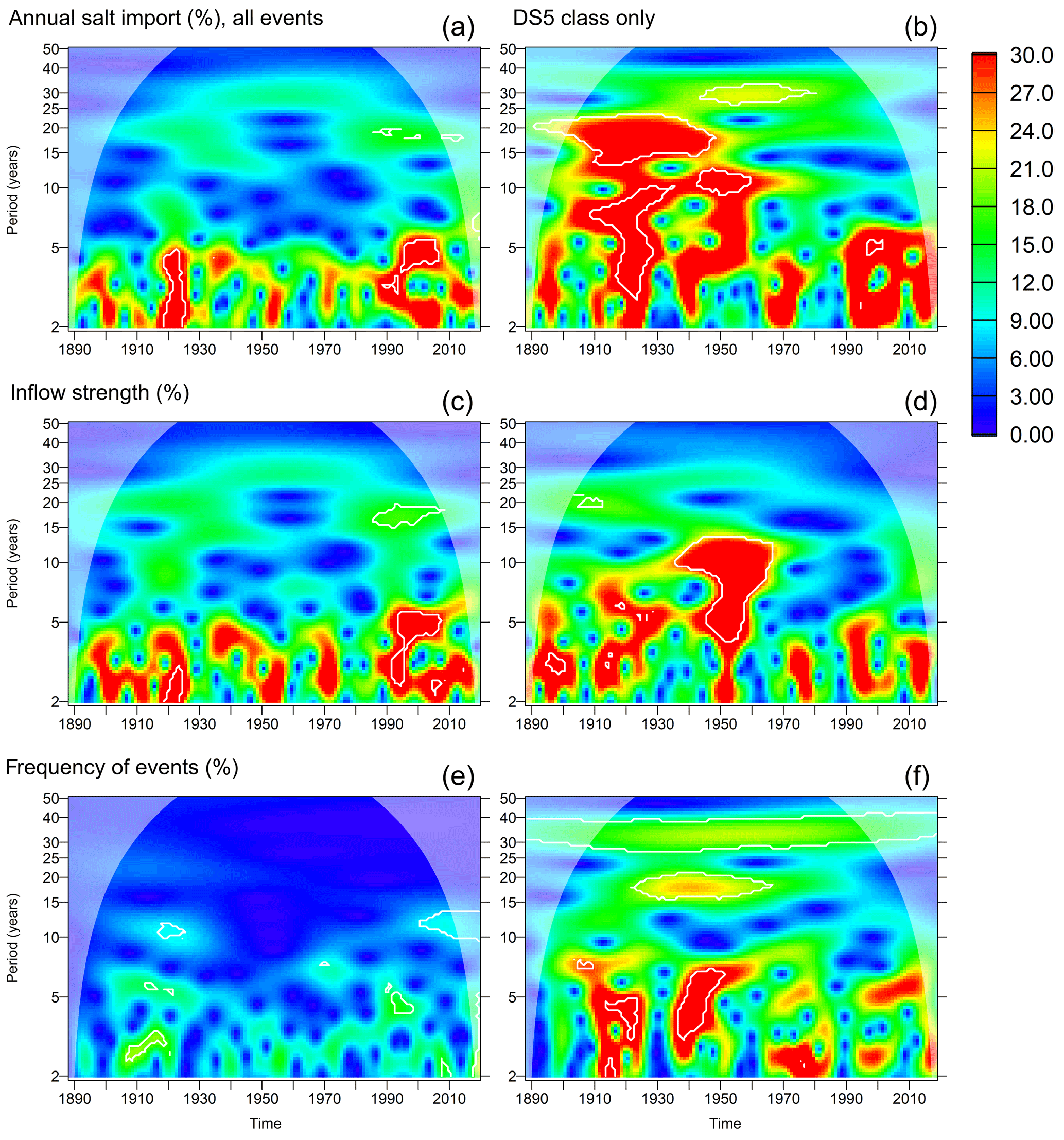
Figure 10 Wavelet analysis of the relative change in inflow activity (%). (a, b) total salt import. (c, d) Inflow strength as mean salt import during a single inflow event. (e, f) Inflow frequency as number of inflows per year.

Figure 10 shows the wavelet decomposition of the salt import across Darss Sill which was caused by the barotropic inflow events found in Mohrholz (2018). Looking at the total import (panel a), we find strong relative deviations of more than 30 % on periods lower than 5 years and smaller deviations on longer timescales; the longest timescale is around 30 years on which a relative change of ±15 % shows up between 1900 and 1990. The relative changes in the salt import by large (DS5 class) inflow events are stronger and intermittently statistically significant for different periods between 3 and 30 years. The 30-year period shows statistically significant energy between 1940 and 1980.

The salt import is determined both by the frequency of the inflow events and their individual strength in terms of the salt import during a single inflow event. Focussing on the 30-year timescale, we find that a change in inflow strength occurs which is strongest between 1940 and 1980. The total frequency of occurrence of all inflow events does, however, not change substantially at multidecadal timescales. In contrast, the frequency of strong (DS5 class) inflow events shows a significant variation in the 30–40-year range for the entire period of the analysis.

Figure 11 Common wavelet power between observed surface and bottom salinity at station BY15 (Eastern Gotland Basin) and normalized annual import of salt by inflow events. (a, c) All inflow events identified in Mohrholz (2018). (b, d) Only DS5 class events. White contours indicate that the WA or CWP is significant at the 95 % confidence level with respect to a random shuffling of the annual means of the salt import. Arrows indicate relative phase: →: in phase; ↓: salt import leading salinity by 90^∘. Thick arrows indicate phase stability (wavelet coherence > 0.95). The region where arrows are not drawn indicates the cone of influence for the common wavelet power; the white shading indicates the cone of influence for the wavelet coherence.

Figure 11 shows the common wavelet power which exists between the observed time series of surface and bottom salinity at Gotland Deep and the salt import during the barotropic events identified by Mohrholz (2018). The salt import time series have been normalized (divided by their standard deviation) such that the common wavelet power directly measures the salinity deviations related to the fluctuations in salt import. CWP between salt import and bottom salinity (bottom row in Fig. 11) exists intermittently for different periodicities above 10 years. For the 30-year period, the common wavelet power is significant for the entire period in which our analysis is outside the cone of influence. Wavelet coherence above 0.95 is frequently observed, especially at the 30-year period, always indicating that the salt import leads the bottom salinity, but with different lag. For the 30-year period, the lag is around 60^∘ which means approximately 5 years. For the surface salinity, common wavelet power on timescales longer than 5 years shows up around the 30-year period only. Here, the lag between salt import and salinity maxima is around 7.5 years.

4.3.3 Salt import at high and low salinities

In the following, model results are discussed instead of observations. Figure 12 shows a wavelet decomposition of the modelled salt imports in different salinity ranges across different transects in the model. We consider the import in the full salinity range above the threshold salinity where typically import equals export, $T_{\widehat{S},t}$ as well the subdivision into the lower and upper salinity range, T_lowsal,t and T_highsal,t.

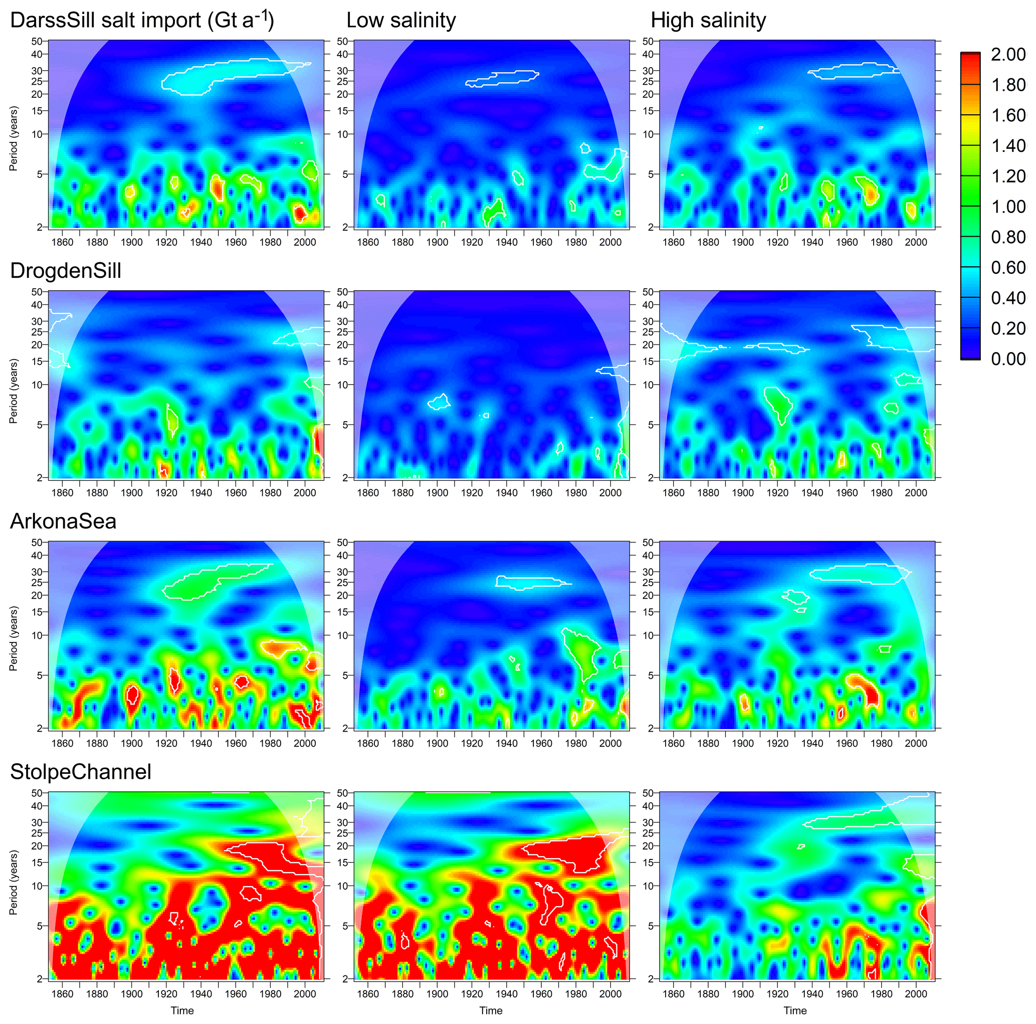
Figure 12 Wavelet amplitudes of net salt import across selected transects. Left column: $T_{\widehat{S},t}$ (transport in all salinities above $\widehat{S}$). Middle column: T_lowsal,t (salinities above $\widehat{S}$ but below $S_{\mathrm{in}}^{\mathrm{50}\mathit{\%}}$). Right column: T_highsal,t (salinities above $S_{\mathrm{in}}^{\mathrm{50}\mathit{\%}}$).

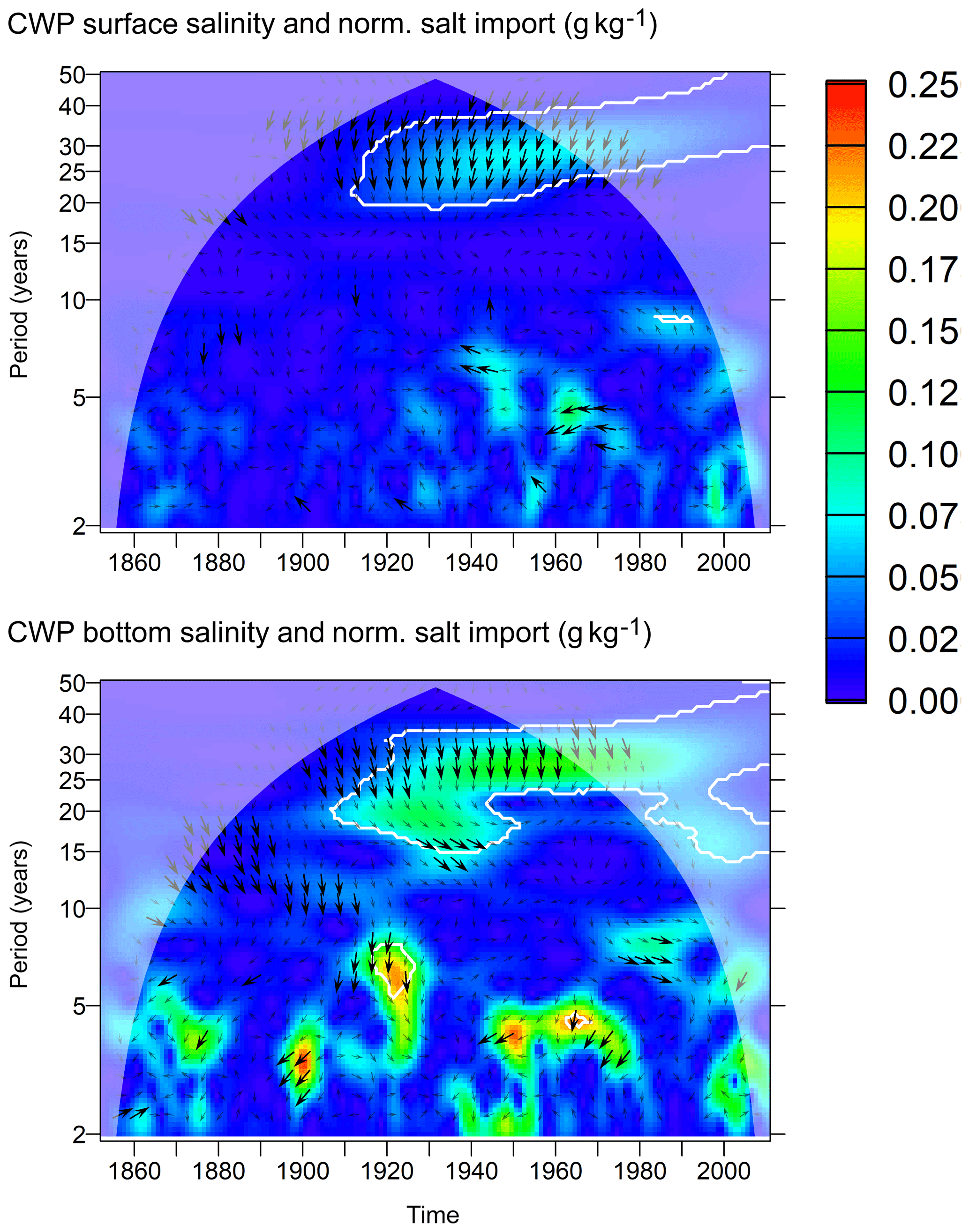
Figure 13 Common wavelet power between modelled surface and bottom salinity at station BY15 (Eastern Gotland Basin) and the normalized time series of $T_{\widehat{S},t}$ across the transect ArkonaSea (g kg⁻¹). White contours indicate that the WA or CWP is significant at the 95 % confidence level with respect to a random shuffling of the annual means of the salt import. Arrows indicate relative phase: →: in phase; ↓: salt import leading salinity by 90^∘. Thick arrows indicate phase stability (wavelet coherence > 0.95).

We find significant wavelet power in the Darss Sill import at the 30-year frequency band from 1920 on. Both low and high salinities contribute to this variation. The Drogden Sill import, in contrast, does not show a 30-year variation; the dominating interdecadal variations occur at lower periods around 20 years here.

The import across the ArkonaSea transect² shows similar patterns to the Darss Sill variations, but the signal increases in magnitude, reflecting an increase in the total volume transport due to entrainment. Transports across Stolpe Channel vary by more than 2 Gt a⁻¹ at lower salinities at different periods up to 20 years. The import at higher salinities (above 11.15 g kg⁻¹), however, shows a similar signal as the import across ArkonaSea in total, with significant energy in the 30-year frequency band from 1930 onwards.

Figure 13 shows the common wavelet power between the normalized salt import $T_{\widehat{S},t}$ across the ArkonaSea transect and the surface or bottom salinity at station BY15 in the numerical model. We see that significant common wavelet power exists in the 30-year frequency band from around 1910 on both for surface and bottom salinities. We can see that the common wavelet power between salt import and bottom salinities is about twice as large compared to surface salinities. This is in line with the empirical results shown in Fig. 11. Wavelet coherence above 0.95 exists in the 30-year frequency band. Here, the salt import leads bottom salinities by 60–90^∘, which means 5–7.5 years, and the surface salinities by more than 90^∘, which means a time lag of around 8 years. For variations with shorter periods up to 10 years, common wavelet power occurs intermittently but is hardly ever statistically significant. The phase relation, however, shows that in cases where phase stability exists, salt import always leads bottom salinity, although at differing lag times. In relation to surface salinity, we find phase lags between 135 and 225^∘, indicating that larger salt imports occur during periods of low surface salinity if timescales below 10 years are considered.

4.3.4 Vertical turbulent mixing

We use the third power of the 10 m wind speed as a proxy for interannual variations in the turbulent kinetic energy production which causes vertical mixing. Figure 14 shows the wavelet analysis of the third-power wind at Gotland Deep and its relation to the modelled surface and bottom salinities. Practically no energy exists at the 30-year period. Common energy between third-power wind and salinities is never significant at the 95 % confidence level. For surface salinity, however, the relative phase shift between wavelets with common energy is always less than ±90^∘ as long as the period is 4 years or longer. This indicates that on these timescales, high surface salinities coincide with strong wind speeds.

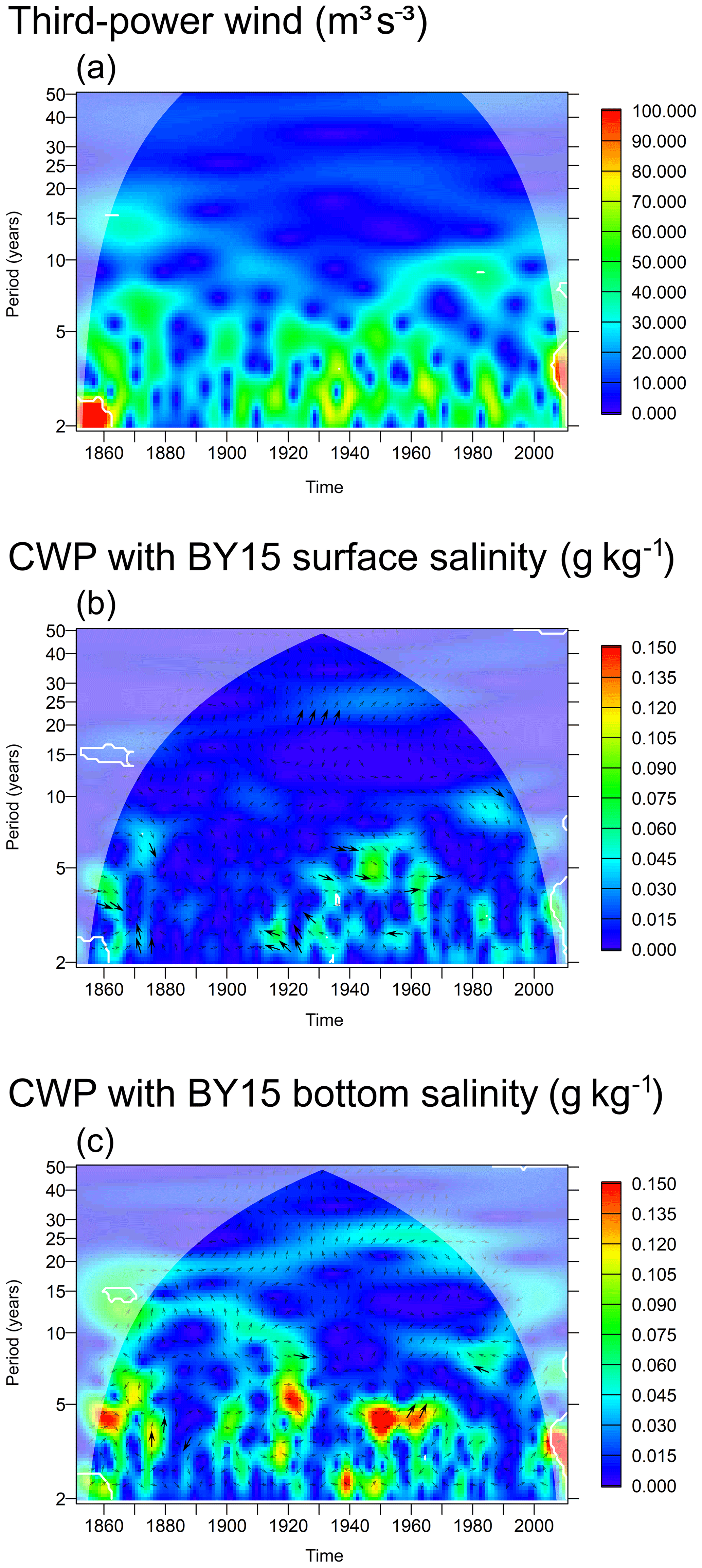
Figure 14 (a) Wavelet amplitude of the third power of the wind speed (m³ s⁻³). (b) Common wavelet power between modelled surface salinity and normalized third-power wind (g kg⁻¹). (c) The same for bottom salinity. All variables at station BY15 (Eastern Gotland Basin). White contours indicate that the WA or CWP is significant at the 95 % confidence level with respect to a random shuffling of the annual means of the third-power wind. Arrows indicate relative phase: →: in phase; ↓: third-power wind leading salinity by 90^∘. Thick arrows indicate phase stability (wavelet coherence > 0.95).

4.4 Coherence between runoff and salt import

Finally, we investigate the common wavelet power between net salt import across the sills and the runoff into the Baltic Sea. As we see in Fig. 15, the common wavelet power between the salt import and the normalized runoff is on the order of 0.5 Gt a⁻¹ for the DarssSill transect on the 30-year timescale. It is substantially lower for Drogden Sill. At the ArkonaSea and StolpeChannel transects, we especially find high common wavelet power if we consider the transports in the high-salinity range only; here we find a similar common variation around 0.5 Gt a⁻¹. Phase stability is very high in the 30-year frequency band, with higher imports across DarssSill taking place during periods of low runoff. At ArkonaSea and StolpeChannel, the salt import slightly lags the lower runoff by about 2 years. If we consider higher frequencies, we intermittently find common wavelet power, partly exceeding 1 Gt a⁻¹ and in several cases statistically significant. The phase relation, where it is stable, always shows an opposite-phase component (a lag of between 90 and 270^∘), indicating that the coincidence between low runoff and high salt import is not restricted to the 30-year frequency band.

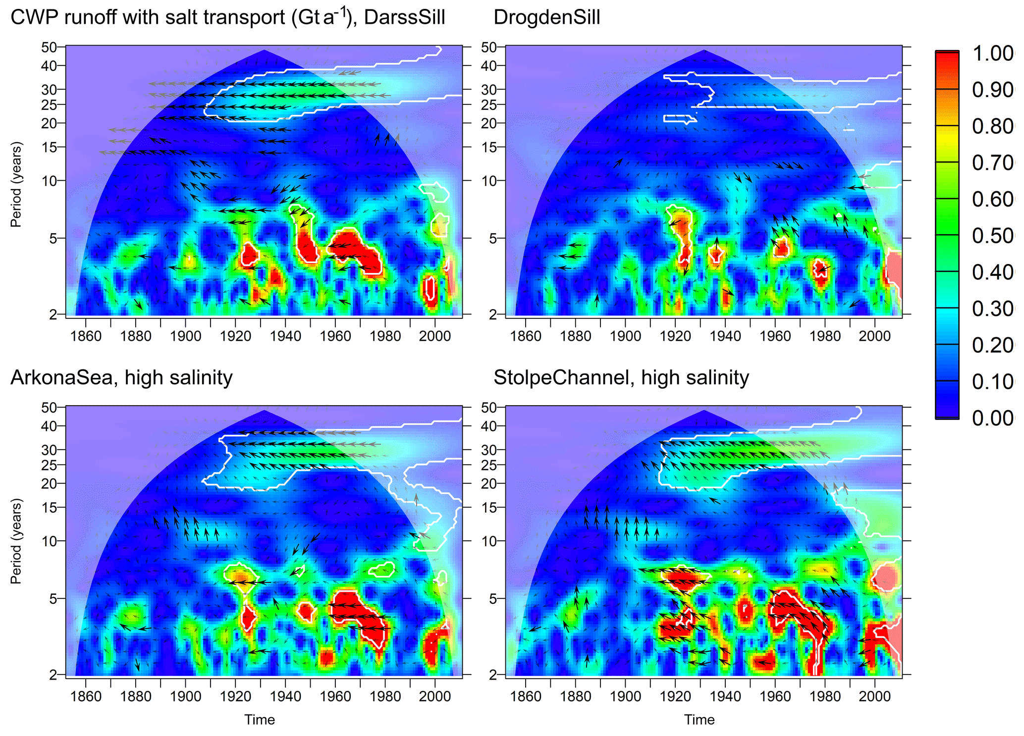
Figure 15 Common wavelet power between salt import across selected transects and normalized annual runoff into the Baltic Sea. $T_{\widehat{S},t}$ is chosen as time series for salt import across DarssSill and DrogdenSill transects, while T_highsal,t is chosen across ArkonaSea and StolpeChannel. White contours indicate that the WA or CWP is significant at the 95 % confidence level with respect to a random shuffling of the annual means of the runoff. Arrows indicate relative phase: →: in phase; ↓: runoff leading salt import by 90^∘. Thick arrows indicate phase stability (wavelet coherence > 0.95).

5 Discussion

5.1 Decadal salinity variations in the Baltic Sea

Wavelet analysis showed that the most relevant timescale on which salinity variations occur in the central Baltic Sea is the 30-year period. Only for this period was permanent significant wavelet power found, both in the observations and in the model (Figs. 6–7). In the western Baltic Sea (Stations BY2 and BY5), interannual variations are stronger anyway but also occur on more variable temporal scales. Observations and the model agree quite well in terms of the timescales at which salinity changes if we visually compare the spectral distributions in Figs. 6 and 7.

In the model, the 30-year oscillation starts to become significant in the first half of the 20th century only; the exact decade depends on the station. Since the observation data start later, we cannot say whether the absence of the oscillations in the 19th century is real or a model artefact. We would like to stress that the wavelet analysis results in the cone of influence should not be interpreted. We see three possible reasons why the model could have missed salinity variations in the 19th century. Firstly, the model may have required a spin-up period from its initialization in 1850 with possibly inconsistent initial conditions. Secondly, the river forcing dataset is not homogenous in time; for 1850–1900 a statistical model was used which was based on atmospheric pressure over land (Hansson et al., 2011). Figure 4 in by Hansson et al. (2011) already indicates that the 30-year variability in the runoff may be underestimated by the statistical model. Finally, the atmospheric forcing dataset may show less realism further back in the past. The analogue method used to create it requires that, for each day in the past climate, there is a matching day in the recent reference period whose values are chosen. The mismatch, e.g. in the wind field, between the actual day and the matching day could be larger if past climate and reference climate differ more strongly, leading to possibly too poor a representation of major Baltic inflow dynamics.

5.2 Drivers of the variations

5.2.1 Climate indices

The comparison with the climate indices shows that neither NAO nor AMO contain the 30-year signal which is apparent in the Baltic Sea salinity throughout the 20th century. Their dominating timescales are substantially different (below 10 years for NAO, above 60 years for AMO), but also the energy they contain at different periods does not match the 30-year period we are interested in, as the change in relative phase over time shows. The NAO index shows some variation in periods around 35 years, while the AMO has energy at 20–25 years.

These frequency differences to the 30-year period are too large to allow for salinity changes being driven by these large-scale atmospheric patterns directly. More accurately phrased, the variability over the North Atlantic which is measured by the indices is most certainly not the driver of the salinity changes throughout the considered period. However, one might speculate that the difference is small enough to have an oscillator with an intrinsic 1∕30-year eigenfrequency excited by these external variations, which then continues to oscillate after the initial forcing ended. So, we cannot rule out that the climate indices play an indirect role in the salinity variations.

5.2.2 Influence of vertical turbulent mixing

As Fig. 14 shows, there is almost no variation in third-power wind at station BY15 with a period around 30 years, so a variation in the generation of turbulent kinetic energy and a corresponding change in the vertical mixing across the halocline can be ruled out as driver of the interdecadal salinity changes.

5.2.3 Runoff and salt import

River runoff and surface salinity show a very similar pattern in their wavelet decomposition at multidecadal timescales (compare Fig. 9 with Fig. 6). Interdecadal salinity variations in the model start at the beginning of the 20th century, which is when they also start in the river forcing. The phase relationship is as expected; periods of low salinity follow those of increased river runoff, at least in the interdecadal variability. What is counterintuitive is that the covariations in the bottom salinity with runoff (a) are stronger than at the surface and (b) are slightly leading the variations in surface salinity (Fig. 9).

The relationship between Baltic Sea salinity and salt import was studied by two different approaches in Figs. 11 and 13: by relating observed salinity changes to the barotropic inflow reconstruction of Mohrholz (2018) and by relating modelled salinity changes to the net salt import above a specific salinity threshold in the model. Since the amount of salt in the Baltic Sea is exactly determined by the salt transports in and out, we should expect the 30-year period from the salinity fluctuations to also occur in the salt import; both methods confirm this thought (Figs. 10 and 12). The phase lag between high salt import and high bottom salinities is around 60^∘ (5 years, somewhat larger in the model); between salt import and surface salinities we find an approximately 90^∘ (7.5 years) phase difference. This means that bottom salinity changes slightly before surface salinity. The fact that it also shows stronger variations than surface salinity indicates that salinity oscillations below the halocline drive those above the halocline, not vice versa as would be expected if the salinity changes were directly controlled by runoff.

The results are in excellent agreement with Meier and Kauker (2003b). They found in a similar model study that the cumulated runoff anomaly excellently explained the decadal changes in mean salinity. However, an additional sensitivity simulation with identical runoff in each year still reproduced the stagnation periods of the 1920s and 1980s. This proves that a driver different from runoff explains part of the decadal variability in salinity. Meier and Kauker (2003b) showed that enhanced zonal wind over the Baltic Sea during stagnation periods both increases precipitation in the catchment and reduces inflow activity. This link between runoff and inflow activity, however, can only explain a part of the decadal variability in salinity. Wavelet analysis of the zonal wind component at the Swedish meteorological station Landsort (SMHI, 2019) indicates that interdecadal variations are prominent on the 20-year rather than the 30-year timescale (not shown).

Since the strong westerly winds are the result of favourably aligned storm tracks, barotropic inflows are considered rather random and unpredictable, so it is not obvious why they show a 30-year variation in their total salt import. Figure 10 shows that it is not the total frequency of the inflow events that changes but the average amount of salt which an individual inflow event transports into the Baltic Sea. This causes the frequency of strong inflows (DS5 events), and correspondingly the total salt flux, to change significantly.

So, both river runoff and the strength of barotropic inflow events show a variation on the 30-year timescale, and both of them show a stable and plausible phase relationship to be the driver of the interdecadal salinity fluctuations. This means that from correlation analysis alone, we cannot tell which of the processes is responsible for which fraction of the salinity change. Asked differently, are interdecadal variations in wind patterns or in precipitation over land responsible for the observed salinity oscillations? This is especially important if the negative covariance between inflow intensity and river runoff was by coincidence in the past and will not continue into the future. Figure 15 shows this very clear opposite-phase relationship between river runoff and salt import across the DarssSill transect (top left panel), but it is not yet known whether a deterministic physical mechanism links the two on the 30-year timescale. The existence of two synchronous mechanisms causing salinity changes in the Baltic Sea complicates the validation of circulation models applied for future climate projections. Verifying that a model was able to capture the multidecadal climate variations in the historical period might not be sufficient to prove that its sensitivity of salinity towards changes in runoff is realistic. Instead, a model could, for example, overestimate the sensitivity of salinity to runoff and underestimate that to changes in wind or vice versa. For climate projections on Baltic Sea freshening, this means an additional source of uncertainty.

The major findings from the wavelet coherence analysis are summarized in Table 2.

Table 2 Summary of the findings of the wavelet coherence analysis.

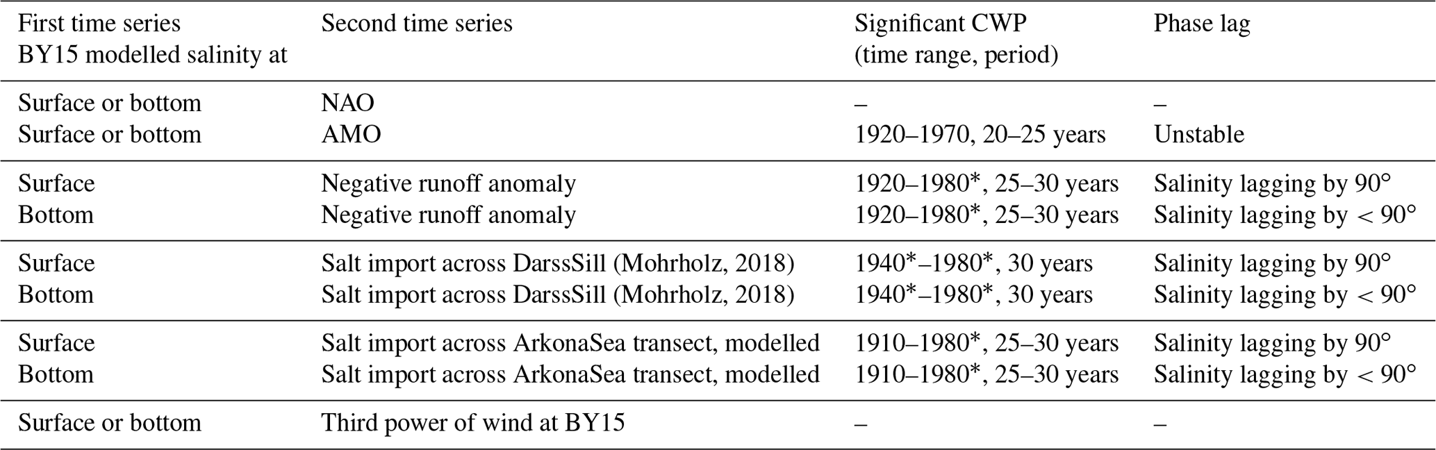
^* Possibly outside this range, since this date is the cone of influence

6 Estimation of the direct dilution effect

We found from the wavelet analysis that varying bottom salinities may drive changes in surface salinities on the 30-year timescale. This is in contrast to the hypothesis that the runoff variations directly control this salinity by freshwater dilution. We will employ a different, complementary method in this section to assess the importance of the direct dilution effect.

Figure 16 Baltic Sea annual mean salinity above the 8.9 g kg⁻¹ isohaline (g kg⁻¹). Black: results of numerical model. Red: after the approximation that the outflow salinity is the mean salinity modified by a factor α. Blue: additionally under the assumption of a constant river runoff.

We can think of at least four pathways in which Baltic Sea salinity would vary at the same frequency as the runoff:

• direct dilution effect – the Baltic Sea loses salt due to an enhanced outflow volume caused by increased runoff and net precipitation (Schott, 1966).

• indirect dilution effect – higher volume and lower salinity of the Baltic outflow due to enhanced river runoff reduces the salinity of inflowing water, e.g. by increased entrainment into the Kattegat deep water (Rodhe and Winsor, 2002) or a northward shift in the salinity front in the Kattegat.

• wind patterns systematically linked to runoff – wind patterns which modify inflow strength could be driven or favoured by the same atmospheric patterns that control the precipitation in the catchment; these variations in salt import could therefore be systematically linked to the river runoff although would not be a consequence of it.

• wind patterns only coincidentally linked to runoff – the link between strong inflows and low river runoff could be just coincidental during the instrumental period.

To estimate the direct dilution effect, we apply the salt budget calculations described in Sect. 2.5. The mean salinity in the Baltic Sea above the isohaline of 8.9 g kg⁻¹, which is the value of $\widehat{S}$ for the ArkonaSea transect, is shown in Fig. 16 for three different models: the full numerical model, the same simplified by assuming a constant ratio α=1.17 between mean salinity and outflowing salinity, and the model assuming both constant α and constant runoff. We find that assuming a constant α does not have a large effect on the mean salinity in the upper layer. The assumption of a constant river runoff, in contrast, has an impact on surface salinity. It reduces the standard deviation of salinity by 10.6 % for the complete time series or by 27.2 % if we consider the period from 1910 only where we find the 30-year oscillations. So, we can estimate that the direct dilution effect is responsible for about one-fourth of the salinity variations in this period. This may be a lower estimate, since the GETM model overestimates surface salinities in general and may therefore underestimate the influence of river water on the surface layer.

7 Conclusions and outlook

7.1 Conclusions

A 159-year hindcast simulation was conducted using the GETM model to understand interdecadal variations in Baltic Sea salinity. Even though the model results show a positive bias in mean salinities which increases from south to north, the interdecadal variations in salinity were captured well by the model, making the simulation results applicable for our study.

A 30-year variability was found in the following quantities:

• surface and bottom salinities at seven different oceanographic stations, both in the model and in observations

• river runoff into the Baltic Sea

• salt transports across Darss Sill, especially during inflow events which last for at least 5 d .

No such variability was found in third-power wind speeds or in the climate indices NAO or AMO.

Runoff is one of the drivers of multidecadal variability of Baltic Sea salinity, but the direct dilution effect was found to be responsible for about one-fourth of the oscillations only. The impact of vertical turbulent mixing on multidecadal variability is small. Salt water inflows contribute to the multidecadal variability in salinity as well, in particular of the bottom layer salinity. Our findings indicate that changes in bottom salinity lead those in surface salinity and not vice versa.

7.2 Outlook

The total effect of runoff on salinity, the sum of the direct and indirect dilution effect, can be determined by sensitivity runs of a numerical model, artificially setting the runoff to constant. Such a sensitivity experiment with climatological river runoff but realistic wind forcing has been conducted by Meier and Kauker (2003b), and interdecadal salinity variations were reduced by about half (Scenario F1 in their Fig. 11). This suggests that if their model and our model agree, both the direct and the indirect effect of river runoff could explain about 50 % of the salinity changes. To find out whether this number (25 % for indirect effect of river runoff) is realistic or a model artefact, one would need to check whether the processes that propagate the outflow water signal to the inflow strength are correctly represented. We will do so in ongoing sensitivity experiments. To identify and quantify these physical mechanisms in model simulations and then verify them in field studies would be an important next step to estimate the vulnerability of Baltic Sea salinity to runoff changes. For example, if entrainment of Baltic outflow water into the Kattegat deep water is identified as a major process in the model, the turbulence parameterization would be critical for realistically estimating this mixing intensity. The discrimination between the wind and runoff effect on salinity might, however, be impossible if non-linear interactions between the two play a significant role, such that their combined effect is different from the sum of both effects individually.

Another important question is whether the wind-driven changes in inflow strength (according to the study of Meier and Kauker (2003b) the remaining 50 % together with inflow frequency) are intrinsically related to changes in runoff. That is, can an atmospheric pattern be identified which at the same time increases precipitation in the Baltic Sea catchment and decreases inflow strength?

The identification of a climate pattern which controls precipitation over the Baltic Sea catchment on a decadal timescale should be of importance not only for ocean science. If an oscillator exists in nature which shows an intrinsic period of 30 years and affects river runoff, its identification would allow predicting trends in river runoff over lead times of a decade. If the present amplitude and phase of the oscillatory pattern could be detected, this decadal lead time would, for example, allow us to initiate engineering measures for river flood protection.

Appendix A: Coordinates of oceanographic stations

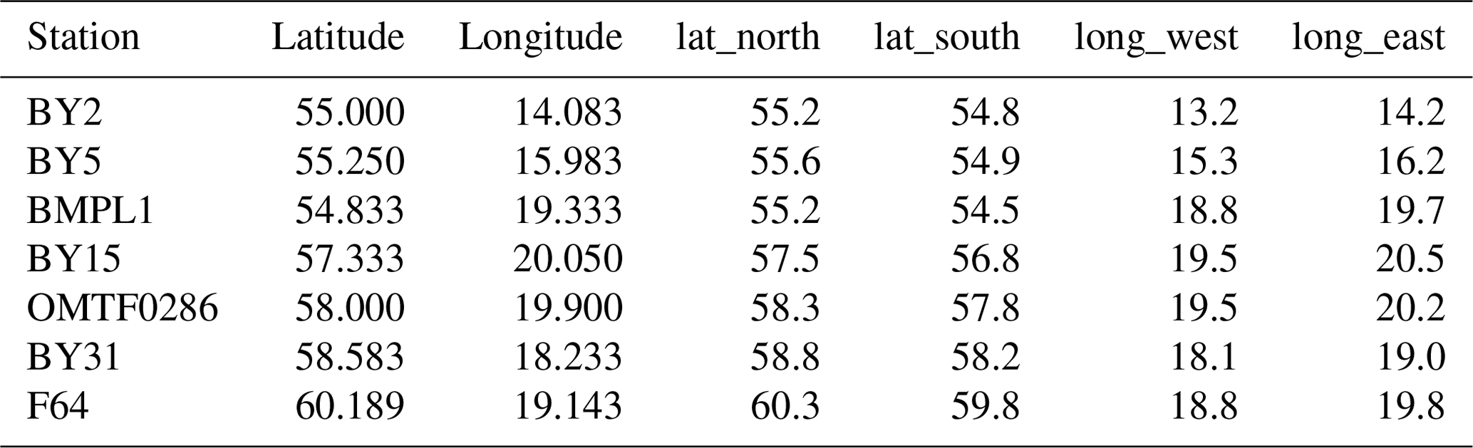
Locations of oceanographic stations and borders of the corresponding boxes for selecting ICES observations are given in Table A1.

Table A1 Locations of oceanographic stations and borders of the corresponding boxes for selecting ICES observations (^∘ N or ^∘ E).

Appendix B: Salinity thresholds for the transects

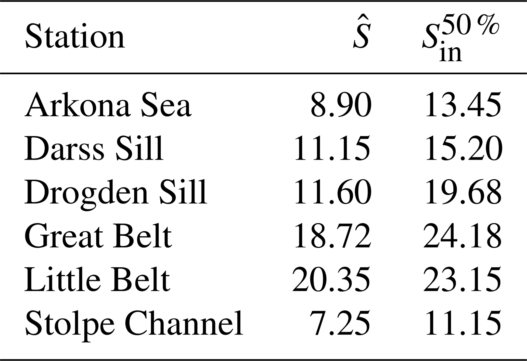
Salinity thresholds for the transects are given in Table B1.

Table B1 Modelled salinity thresholds for selected transects (g kg⁻¹).

Appendix C: Details on model setup

Three sub-grid-scale parameterizations are applied in the model.

• Firstly, turbulent vertical diffusivity and viscosity are calculated by the General Ocean Turbulence Model (GOTM, https://gotm.net/, last access: 18 August 2020). A second-order Mellor-Yamada model is used (Mellor and Yamada, 1982; Umlauf and Burchard, 2005), which solves dynamic equations for turbulent kinetic energy (TKE, k) and a turbulence length scale L. To derive vertical mixing efficiencies from these, we use coefficients given by Canuto et al. (2001).

• Secondly, turbulent horizontal diffusivity and viscosity are prescribed by a Smagorinsky scheme (Smagorinsky, 1963). Since the model uses terrain-following coordinates, the Smagorinsky mixing is not strictly horizontal but contains a vertical component, especially at sloping topography. So, this numerical scheme can also be used to parameterize boundary mixing, which is the major component for vertical diffusion in the deep areas of the central Baltic Sea (Holtermann et al., 2012). To account for this, we set the Prandtl number for the turbulent horizontal exchange to 4.

• Finally, we parameterize the effect of Langmuir circulation (Langmuir, 1938) on vertical mixing. The approach follows Axell (2002). Langmuir circulations are included as an additional production term for TKE. Its input is proportional to the third power of the 10 m wind speed.

The model includes a thermodynamic sea ice model (Winton, 2000), but no dynamic component, i.e. ice drift and especially the increase in ice thickness due to drift-induced ridging and rafting (Mårtensson et al., 2012), is explicitly represented. Since this implies that the model would underestimate ice thicknesses and the ice-covered period, we introduce empirical correction factors to the freezing and melting processes. While ice growth is accelerated by a factor of 1.9, the melting of ice is decelerated by the same factor. This also accounts for the unresolved ice–ocean boundary layer.

Measurements of ocean salinity are scarce in the 19th century and, to the best of our knowledge, completely lacking in the Baltic Sea for the first model year, 1850. As a result, defining initial conditions for the model is not straightforward. We use measurements from the year 1979 and extrapolate them to the model grid. This rather arbitrary choice obviously induces a substantial amount of uncertainty, especially for the first decades. However, the unavoidable deviations from the unknown reality can be expected to decrease over a timescale of about 30–40 years, which is the typical timescale in which Baltic Sea water is renewed by inflows from the Kattegat (Meier, 2007).

Appendix D: Details on wavelet analysis

For the dimensionless shape parameter in the Morlet wavelet, we choose a standard value of ω₀=6 as suggested by Grinsted et al. (2004), so the oscillatory term in Eq. (9) has a period of $T=\mathrm{2}\mathit{\pi }a/\mathrm{6}\approx \mathrm{1.05}a$ (Fig. D1). The scaling factor in Eq. (9) is chosen in such a way that the wavelet transform of any of the two functions,

$$\begin{array}{}\text{(D1)}& f_{\mathrm{1}}\left(t\right)=b\sin (\mathrm{2}\mathit{\pi }t/T),f_{\mathrm{2}}\left(t\right)=b\cos (\mathrm{2}\mathit{\pi }t/T),\end{array}$$

gives a wavelet amplitude $\left|W\right(a,t\left)\right|$ equal to b; see the proof in the Supplement. The wavelet transform measures the correlation between the signal and the wavelet. A value of $W(a,t)=b$ means that the analysed time series shows the same correlation with the wavelet as a harmonic function with amplitude b. A value different from 0 does not necessarily mean that a periodic signal was detected at time t; it just means the signal shows some similarity to the wavelet. Since the wavelet is complex, Re(b) describes the correlation with the real part of ϕ and Im(b) describes the correlation with the negative imaginary part of ϕ, so arg(b) contains the phase information. When we perform wavelet transforms of ICES observation data, we use the deseasonalized annual means and fill the gaps in the time series by linear interpolation.

To check whether wavelet amplitude (WA) or common wavelet power (CWP) are significant, we generate an ensemble of randomized time series, created by shuffling the years of the original time series. For CWP, we only shuffle the second (the explanatory) time series. Then we calculate the time average of the 95th percentile of the randomized WA or CWP, giving a critical value for each frequency. Where the signal exceeds this threshold, it is regarded as significant.

For the averaging operator in the wavelet coherence calculations, we choose a simple box average over the intervals $t\in [t-a,t+a]$ and $a\in [a-a/\mathrm{8},a+a/\mathrm{8}]$ in Eq. (12).

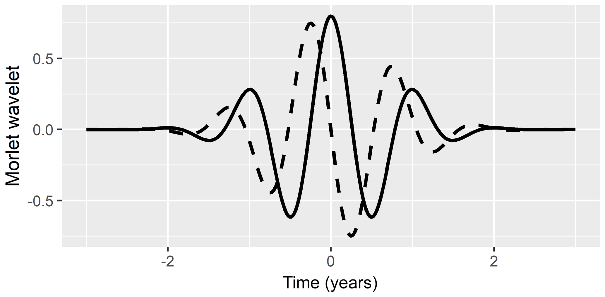
Figure D1 The Morlet wavelet for the temporal scale a=1 year and ω₀=6. Solid line: real part. Dashed line: imaginary part. Please note that the periodicity almost matches the temporal scale.

Appendix E: Discussion of the differences between stations in explained variance of the bottom salinity time series

Baltic Sea bottom salinity is controlled by inflowing water from the North Sea. This water passes a series of sills under favourable meteorological conditions and is diluted on its pathway by the intrusion of ambient water. One might therefore expect that the mismatch between reality and model in the bottom salinity increases with increasing distance to the North Sea, since errors accumulate across this path.

The explained variance on a decadal scale (see Table 1) shows the opposite: it decreases from Arkona Sea (BY2, 13 %) to Bornholm Sea (BY5, −56 %) but increases again in the central Baltic to reach its maximum value (BY15, 52 %). The negative explained variance at BY5 arises in spite of a small positive correlation between model and observations (R=0.44), but the model overestimates the variance in the salinity by a factor of 1.74.

One possible explanation for this paradox is that it is not the bottom salinity in one basin that controls the salt inflow into the next one, but rather the salinity at the sill depth. If we consider salinity at 60 m depth at station BY5, we actually get a positive value for explained variances of 22 % (interdecadal) and 34 % (interannual), which shows that the deviation between model and observations is larger than the signal of the observations itself only for the salinity in the very deepest part of the Bornholm Basin (93 m deep).

The fact that the interdecadal variation is still captured best in the Eastern Gotland Basin might indicate that the volume transports are actually more important than the salinities for determining the salt flux into the basin. During single inflow events, it is crucial that the salinity of an inflowing plume is high enough to change the bottom salinity. On a decadal scale, less dense inflows that show interleaving (reaching a depth below the halocline but not the deepest part of the basin) may also change the bottom salinity indirectly by reducing the vertical upward diffusion of salt.

Another possible explanation is that processes inside the Baltic Sea effectively control its decadal bottom salinity, such that the inflow process plays a less important role on these timescales. It remains speculative which processes can play this role, but mixing processes controlling the halocline strength could plausibly influence bottom salinity. While we showed that the third power of the wind as a proxy for the direct wind work does not show energy in the frequency band of interest, a variation in, for example, upwelling intensity and correspondingly mesoscale activity could represent such a local control mechanism. Identifying such possible local influences on bottom salinity will require more detailed investigations.