Lessons from a high-CO₂ world: an ocean view from  ∼ 3 million years ago

A range of future climate scenarios are projected for high atmospheric CO₂ concentrations, given uncertainties over future human actions as well as potential environmental and climatic feedbacks. The geological record offers an opportunity to understand climate system response to a range of forcings and feedbacks which operate over multiple temporal and spatial scales. Here, we examine a single interglacial during the late Pliocene (KM5c, ca. 3.205±0.01 Ma) when atmospheric CO₂ exceeded pre-industrial concentrations, but were similar to today and to the lowest emission scenarios for this century. As orbital forcing and continental configurations were almost identical to today, we are able to focus on equilibrium climate system response to modern and near-future CO₂. Using proxy data from 32 sites, we demonstrate that global mean sea-surface temperatures were warmer than pre-industrial values, by ∼2.3 ^∘C for the combined proxy data (foraminifera Mg∕Ca and alkenones), or by ∼3.2–3.4 ^∘C (alkenones only). Compared to the pre-industrial period, reduced meridional gradients and enhanced warming in the North Atlantic are consistently reconstructed. There is broad agreement between data and models at the global scale, with regional differences reflecting ocean circulation and/or proxy signals. An uneven distribution of proxy data in time and space does, however, add uncertainty to our anomaly calculations. The reconstructed global mean sea-surface temperature anomaly for KM5c is warmer than all but three of the PlioMIP2 model outputs, and the reconstructed North Atlantic data tend to align with the warmest KM5c model values. Our results demonstrate that even under low-CO₂ emission scenarios, surface ocean warming may be expected to exceed model projections and will be accentuated in the higher latitudes.

1 Introduction

By the end of this century, projected atmospheric CO₂ concentrations range from 430 to >1000 ppmv depending upon future emission scenarios (IPCC, 2014a). At the current rate of emissions, global mean temperatures are projected to exceed 1.5 and 2 ^∘C above pre-industrial values in 10 and 20 years, respectively, passing the targets set by the Paris Agreement (IPCC, 2019). The geological record affords an opportunity to explore key global and regional climate responses to different atmospheric CO₂ concentrations, including those which extend beyond centennial timescales (Fischer et al., 2018). Palaeoclimate models indicate that climates last experienced during the mid-Piacenzian stage of the Pliocene (3.1–3.3 Ma) will be surpassed by 2030 CE under high-emission scenarios (Representative Concentration Pathway, RCP8.5) or will develop by 2040 CE and be sustained thereafter under more moderate emissions (RCP4.5; Burke et al., 2018).

The late Pliocene thus provides a geological analogue for climate response to moderate CO₂ emissions. However, the magnitude of tropical ocean warming differs between proxy reconstructions (e.g. Zhang et al., 2014; O'Brien et al., 2014; Ford and Ravelo, 2019; Tierney et al., 2019a), and stronger polar amplification has been consistently recorded in proxy data compared to models (Haywood et al., 2013, 2016a). Some of the disagreements may reflect non-thermal influences on temperature proxies (e.g. secular evolution of seawater Mg∕Ca; Medina-Elizalde et al., 2008; Evans et al., 2016) and/or seasonality in the recorded signals (e.g. Tierney and Tingley, 2018). It has also been proposed that previous approaches to integrating Pliocene sea-surface temperature (SST) data may have introduced bias to data–model comparison (Haywood et al., 2013). For example, the Pliocene Research Interpretation and Synoptic Mapping (PRISM) project generated warm peak averages within specified time windows (Fig. 1) (outlined in Dowsett et al., 2016, and references therein). However, by integrating multiple warm peaks within the 3.1–3.3 Ma mid-Piacenzian data synthesis windows (Fig. 1), regional and time-transgressive responses to orbital forcing (Prescott et al., 2014; Fischer et al., 2018; Hoffman et al., 2017; Feng et al., 2017) are potentially recorded in the proxy data, which may not align with the more narrowly defined time interval being modelled (Haywood et al., 2013; Dowsett et al., 2016).

Here, we present a new, globally distributed synthesis of SST data for the mid-Piacenzian stage, addressing two concerns. First, we minimise the impact of orbital forcing on regional and global climate signals by synthesising data from a specific interglacial stage: a 20 kyr time slice centred on 3.205 Ma (KM5c; see Fig. 1). At 3.205 Ma, both seasonal and regional distributions of incoming insolation are close to modern values, making this time an important analogue for 21st-century climate (Haywood et al., 2013). The low variability in orbital forcing through KM5c minimises the potential for time-transgressive regional signals to be a feature of the geological data (Haywood et al., 2013; Prescott et al., 2014). Second, we provide a range of estimates from different SST proxies, taking into consideration the uncertainties in proxy-to-temperature calibrations and/or secular processes that may bias proxy estimates. This synthesis is possible due to robust stratigraphic constraints placed on the datasets by the PAGES-PlioVAR working group (see Sect. 2.2).

Figure 1 The KM5c interglacial during the late Pliocene (3.195–3.215 Ma). Upper part of graph: benthic oxygen isotope stack (solid line: LR04, Lisiecki and Raymo, 2005; dashed line and grey shading: Prob-stack mean and 95 % confidence interval, respectively, Ahn et al., 2017). Selected Marine Isotope Stages (KM2 through to M2) are highlighted. The KM5c interval of focus here is indicated by the shaded blue bar. Previous Pliocene synthesis intervals are also shown: PRISM3 (3.025–3.264 Ma) and PRISM4 (isotope stages KM5c–M2; Dowsett et al., 2016). Lower part of graph: reconstructed atmospheric CO₂ concentrations (Foster et al., 2017). Points show mean reported data (except white crosses: median values from Martinez-Boti et al., 2015); shading shows reported upper and lower estimates. Past and projected atmospheric CO₂ concentrations highlighted by arrows: PlioMIP2 simulations are run with CO₂ at 400 ppmv (Haywood et al., 2020) close to the annual mean in 2018 (NOAA). Pre-industrial values from ice cores (Loulerge et al., 2008) and projected representative concentration pathways (RCP) for 2100 CE (IPCC, 2013).

2 Methods

2.1 The KM5c interglacial

KM5c (also referred to as KM5.3) is an interglacial centred on a ∼100 kyr window of relatively depleted benthic ¹⁸O values, which immediately follows a pronounced δ¹⁸O peak during the glacial stage M2 (3.3 Ma; Fig. 1). Minor changes to orbital forcing during KM5 enables a wider target zone (3.205 Ma±20 kyr) for data collection because the potential for orbitally forced regional and time-transgressive climate signals is minimised (Haywood et al., 2013). A comparable approach has been adopted by the PRISM4 synthesis (3.190 to 3.220 Ma; Foley and Dowsett, 2019; see Fig. 1). Here, we focus on a narrow time slice from 3.195 to 3.215 Ma, to span approximately one precession cycle. The reconstructed atmospheric CO₂ concentrations from boron isotopes in KM5c are 360±55 ppmv (for median boron-derived values (n=3), full range: 289–502 ppmv, Fig. 1; Foster et al., 2017). A wider range of atmospheric CO₂ concentrations has been reconstructed for the whole mid-Piacenzian stage (356±65 ppmv for median values (n=36), full range: 185–592 ppmv; Foster et al., 2017).

2.2 Age models

The PAGES-PlioVAR working group agreed on a set of stratigraphic protocols to maximise confidence in the identification and analysis of orbital-scale variability within the mid-Piacenzian stage (McClymont et al., 2017). Sites were only included in the synthesis if they had either (i) ≤10 kyr resolution benthic δ¹⁸O data which could be (or had been) tied to the LR04 stack (Lisiecki and Raymo, 2005) or the HMM-Stack (Ahn et al., 2017) and/or (ii) the palaeomagnetic tie points for upper Mammoth (C2An.2n (b) at 3.22 Ma) and lower Mammoth (C2An.3n (t) at 3.33 Ma). At one site (ODP Site 1090) these conditions were not met (see Supplement), but tuning to LR04 had been made using a record of dust concentrations under the assumption that higher dust flux occurred during glacials as observed during the Pleistocene (Martinez-Garcia et al., 2011). At ODP Site 806, uncertainty over age control resulted from the absence of an agreed splice across the multiple holes drilled by ODP, and a new age model has been constructed (see Supplement). For some sites (see online summary at https://pliovar.github.io/km5c.html, last access: 30 June 2020), revisions to the published age model were made, for example if the original data had been published prior to the LR04 stack (Lisiecki and Raymo, 2005) or prior to revisions to the palaeomagnetic timescale (Gradstein et al., 2012). In total, data from 32 sites were compiled, extending from 46^∘ S to 69^∘ N (Fig. 2).

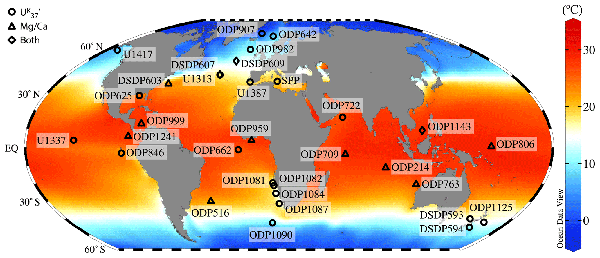
Figure 2 Locations of sites used in the synthesis, overlain on mean annual SST data from the World Ocean Atlas 2018 (Locarnini et al., 2018). A full list of the data sources and proxies applied per site are available in Tables S3 (${\mathrm{U}}_{\mathrm{37}}^{{\mathrm{K}}^{\prime }}$) and S4 (Mg∕Ca) in the Supplement and can be accessed at https://pliovar.github.io/km5c.html (last access: 30 June 2020). The combined PlioVAR proxy data and their sources are also archived at Pangaea: https://doi.pangaea.de/10.1594/PANGAEA.911847.

2.3 Proxy SST data

A multi-proxy approach was taken, to maximise the information available on changing climates and environments during the KM5c interval. Two SST proxies were analysed: the alkenone-derived ${\mathrm{U}}_{\mathrm{37}}^{{\mathrm{K}}^{\prime }}$ index (Prahl and Wakeham, 1987) and foraminifera calcite Mg∕Ca (Delaney et al., 1985). Both proxies have several calibrations to modern SST: here we explore the impact of calibration choice on KM5c SST data, by comparing and contrasting outputs between proxies and between calibrations. Although the TEX₈₆ proxy (Schouten et al., 2002) has also been used to generate mid-Piacenzian SSTs (e.g. O'Brien et al., 2014; Petrick et al., 2015; Rommerskirchen et al., 2011), these data are not included here because they could not be confidently assigned to the KM5c interval either due to low sampling resolution and/or because our age control protocol was not met.

2.3.1 Alkenone SSTs (the ${\mathrm{U}}_{\mathrm{37}}^{{\mathrm{K}}^{\prime }}$ index)

The majority of the 23 alkenone-derived SST datasets included in the PlioVAR synthesis used the ${\mathrm{U}}_{\mathrm{37}}^{{\mathrm{K}}^{\prime }}$ index and applied the linear core-top calibration (60^∘ S–60^∘ N) (Müller et al., 1998) (hereafter Müller98; Tables S2 and S3). The Müller98 calibration applies the best fit between core-top ${\mathrm{U}}_{\mathrm{37}}^{{\mathrm{K}}^{\prime }}$ and modern SSTs, recorded at the sea surface (0 m water depth) and consistent with haptophyte productivity in the photic zone. The sedimentary signal is proposed to record annual mean SST based on linear regression (Müller et al., 1998). Cultures of one of the dominant haptophytes, Emiliania huxleyi, generated only minor differences in the slope of the ${\mathrm{U}}_{\mathrm{37}}^{{\mathrm{K}}^{\prime }}$–temperature relationship (Table S2), where growth temperature was used for calibration (Prahl et al., 1988). Several PlioVAR datasets were originally published using the Prahl et al. (1988) calibration (Table S3).

A recent expansion of the global core-top database (<70^∘ N) was accompanied by Bayesian statistical analysis to assess the relationship(s) between predicted (from ${\mathrm{U}}_{\mathrm{37}}^{{\mathrm{K}}^{\prime }}$) and recorded ocean temperatures (Tierney and Tingley, 2018). The revised ${\mathrm{U}}_{\mathrm{37}}^{{\mathrm{K}}^{\prime }}$ calibration, BAYSPLINE, addresses non-linearity in the ${\mathrm{U}}_{\mathrm{37}}^{{\mathrm{K}}^{\prime }}$-SST relationship at the high end of the calibration, i.e. in the low-latitude oceans (Pelejero and Calvo, 2003; Sonzogni et al., 1997). BAYSPLINE also highlights scatter between predicted and observed SSTs at the high latitudes and explicitly reconstructs seasonal SSTs>45^∘ N (Pacific) and >48^∘ N (Atlantic) and in the Mediterranean Sea (Tierney and Tingley, 2018).

To test the impact of different alkenone temperature calibrations on the quantification of mid-Piacenzian SSTs, we converted all ${\mathrm{U}}_{\mathrm{37}}^{{\mathrm{K}}^{\prime }}$ data to SSTs using both the Müller98 calibration and the BAYSPLINE calibration. For most sites, BAYSPLINE was run with the recommended setting for the prior standard deviation scalar (pstd) of 10 (Tierney and Tingley, 2018). At high ${\mathrm{U}}_{\mathrm{37}}^{{\mathrm{K}}^{\prime }}$ values (above ∼24 ^∘C) it is recommended to use the more restrictive value of 5, to minimise the possibility of generating unrealistic SSTs (e.g. >40 ^∘C) given that the slope of the ${\mathrm{U}}_{\mathrm{37}}^{{\mathrm{K}}^{\prime }}$–temperature calibration becomes attenuated (Tierney and Tingley, 2018).

2.3.2 Foraminifera Mg∕Ca

The magnesium-to-calcium ratio of foraminifera calcite can be used to reconstruct sea-surface (surface dwelling), thermocline (subsurface dwelling), and deep (benthic) ocean temperatures (Delaney et al., 1985; Elderfield et al., 1996; Rosenthal et al., 1997). The PlioVAR dataset includes analysis from 12 sites, on surface-dwelling foraminifera Globigerinoides ruber, Trilobatus sacculifer, and Globigerina bulloides (Table S4). In the original publications, data were converted to SST using a range of calibrations as well as corrections for CaCO₃ dissolution in the water column and sediments, which leads to preferential removal of Mg from the CaCO₃ lattice (generating cooler SSTs than expected; Dekens et al., 2002; Regenberg et al., 2006, 2009). The evolution of the Mg∕Ca of seawater (Mg∕Ca_seawater) over geological timescales may also impact Mg∕Ca-based palaeo-temperature reconstructions (Brennan et al., 2013; Coggon et al., 2010; Fantle and DePaolo, 2005; Gothmann et al., 2015; Horita et al., 2002; Lowenstein et al., 2001). Changes in Mg∕Ca_seawater impact the intercept and potentially the sensitivity of palaeotemperature equations (Evans and Müller, 2012; Medina-Elizalde and Lea, 2010), but there remains uncertainty over the magnitude of Mg∕Ca_seawater changes in the late Pliocene (O'Brien et al., 2014; Evans et al., 2016).

To test the impact of different foraminifera Mg∕Ca SST calibrations on mid-Piacenzian SSTs, we compare published SSTs with the recently developed BAYMAG calibration (Tierney et al., 2019b). We use published SSTs because the original researchers used their best judgement to choose a particular Mg∕Ca-SST calibration, given that it (i) fitted modern (regional) core-top values; (ii) accounted for known environmental impacts (e.g. $\left[{\mathrm{CO}}_{\mathrm{3}}^{\mathrm{2}-}\right]$ correction); (iii) was developed within a particular research group; and/or (iv) fitted conventional wisdom at the time. BAYMAG uses a Bayesian approach that incorporates laboratory culture and core-top information to generate probabilistic estimates of past temperatures. BAYMAG assumes a sensitivity of Mg∕Ca to salinity, pH, and saturation state at each core site and also accounts for Mg∕Ca_seawater evolution through a linear scaling (i.e. there is no change in the sensitivity of the palaeo-temperature equation as Mg∕Ca_seawater evolves) (Tierney et al., 2019b). For each site with Mg∕Ca data, we computed SSTs using BAYMAG's species-specific hierarchical model. In the absence of knowledge concerning changes in salinity, pH, and saturation state in the Pliocene, we assumed that these values were the same as today. We drew seasonal sea-surface salinity from the World Ocean Atlas 2013 product (Boyer et al., 2013) and pH and bottom water saturation state from the GLODAPv2 product (Lauvset et al., 2016; Olsen et al., 2016). We used a prior standard deviation of 6 ^∘C for all sites.

2.4 Climate models

The model outputs used here were generated from the 15 models that contribute to the Pliocene modelling intercomparison project, Phase 2 (PlioMIP2) (Haywood et al., 2020). The boundary conditions for the experiments and their large-scale results for Pliocene and pre-industrial climates are detailed elsewhere (Haywood et al., 2020, 2016b), so they are briefly outlined here.

The Pliocene simulations are intended to represent KM5c (∼3.205 Ma) and were forced with PRISM4 boundary conditions (Haywood et al., 2016b). Atmospheric CO₂ concentration was set to 400 ppmv (Haywood et al., 2020), in line with the upper estimates of atmospheric CO₂ from boron isotope data (Fig. 1; Foster et al., 2017). Lower estimates from the alkenone carbon isotope proxy (Fig. 1) are likely to reflect an insensitivity of this proxy to atmospheric CO₂ in the Pliocene (Badger et al., 2019). All other trace gases, orbital parameters, and the solar constant were specified to be consistent with each model's pre-industrial experiment. The Greenland Ice Sheet was confined to high elevations in the eastern Greenland mountains, covering an area approximately 25 % of the present-day ice sheet. The Antarctic ice sheet has no ice over West Antarctica. The reconstructed PRISM4 ice sheets have a total volume of 20.1×10⁶ km³, equating to a sea-level increase relative to the present day of less than ∼24 m (Dowsett et al., 2016).

Modelling groups had some choices regarding the exact implementation of boundary conditions; however, 14 of the 15 models used the “enhanced” PRISM4 boundary conditions (Dowsett et al., 2016) which included all reconstructed changes to the land–sea mask and ocean bathymetry. Key ocean gateway changes relative to modern values are the closure of the Bering Strait and Canadian archipelago, and the exposure of the Sunda and Sahul shelves (Dowsett et al., 2016). The initialisation of the experiments varied between models (Haywood et al., 2020). Some models were initialised from a pre-industrial state while others were initialised from the end of a previous Pliocene simulation or another warm state. The simulations reached equilibrium towards the end of the runs as per PlioMIP2 protocol.

2.5 Statistical analysis (calculating of global means and meriodional gradients)

For all anomaly calculations we obtain pre-industrial SST from the NOAA-ERSST5 dataset for the years 1870–1899 CE (Huang et al., 2017), ensuring alignment between the KM5c proxy data and the KM5c model experiments (Haywood et al., 2020). This pre-industrial time window excludes the largest cooling linked to the Little Ice Age and predates the onset of 20th-century warming (Owens et al., 2017; PAGES2k Consortium, 2017). The global mean SST anomaly from the proxy data was obtained as follows: firstly, the SST anomaly between the proxy data and the NOAA-ERSST5 data was obtained for each location and the data collated into bins of 15^∘ of latitude. It is assumed that the average of all the data in each bin represents the average SST anomaly for that latitude band. Next, the area of the ocean surface for each bin is obtained. The average SST anomaly is then the average of all the bins weighted by the ocean area in the relevant latitude band.

Meridional gradients were obtained in a similar way. A low-latitude SST anomaly was obtained as the weighted average of all the bins containing low-latitude SSTs (for example the $\mathrm{4}{}^{\circ }\times \mathrm{15}{}^{\circ }$ bins containing latitudes of 30^∘ S–30^∘ N). A high-latitude SST anomaly was obtained as the weighted average of all bins containing high-latitude SSTs (>60^∘ N because there were no proxy data points >60^∘ S). As only the Atlantic Ocean contained data points poleward of 65^∘ N, the high-latitude region used in the gradient calculations for both proxies and models was focused on the longitudinal window from 70^∘ W to 5^∘ E. The meridional gradient SST anomaly is then the low-latitude SST anomaly minus the high-latitude SST anomaly, relative to the pre-industrial period.

There are some uncertainties in this calculation of the global mean SST, in particular, the fact that the proxy data are not evenly distributed throughout a latitude bin and also that some bins contain very few data points. There is a higher density of data in the Atlantic Ocean compared to the Indian Ocean and Pacific Ocean, and no high-latitude data are available to consider a Southern Ocean response (Fig. 2). Nevertheless, this method of calculating averages does attempt to account for unevenly distributed data and provides an SST anomaly (SSTA) that is comparable with model results. The impact of proxy choice was examined in the calculation of the global means and meridional SST gradients. As no Mg∕Ca data were available >50^∘ N or >30^∘ S, we calculated global mean SST and the meridional SST gradients either including or excluding the Mg∕Ca data; both results are outlined below and shown in Table 1.

Table 1 Comparison of the magnitude of the global SST anomaly and meridional SST gradients between KM5c and the pre-industrial period, depending on proxy combination, and the latitudinal bands used for the gradient calculations.

3 Results

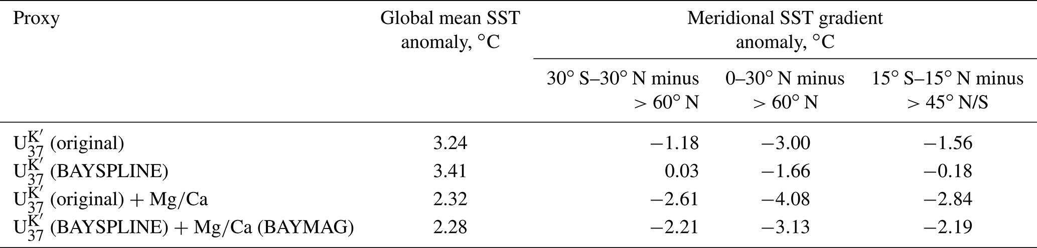
Relative to the pre-industrial period, the combined ${\mathrm{U}}_{\mathrm{37}}^{{\mathrm{K}}^{\prime }}$ and Mg∕Ca proxy data, using the original calibrations, indicate a KM5c global mean SST anomaly of +2.3 ^∘C and a meridional SST gradient reduced by 2.6 ^∘C (Fig. 3). The amplitude of the global SST mean anomaly in the combined proxy data exceeds those indicated in 10 of the PlioMIP2 models but is lower than the global SST anomaly from 6 models. The meridional temperature gradient anomalies are more comparable (Fig. 3). If only the ${\mathrm{U}}_{\mathrm{37}}^{{\mathrm{K}}^{\prime }}$ data are used, the global mean SST anomaly from proxies is higher than all but three of the PlioMIP2 models, and the ${\mathrm{U}}_{\mathrm{37}}^{{\mathrm{K}}^{\prime }}$ meridional gradient calculations are smaller than all models (BAYSPLINE) or one model (original calibration; Fig. 3).

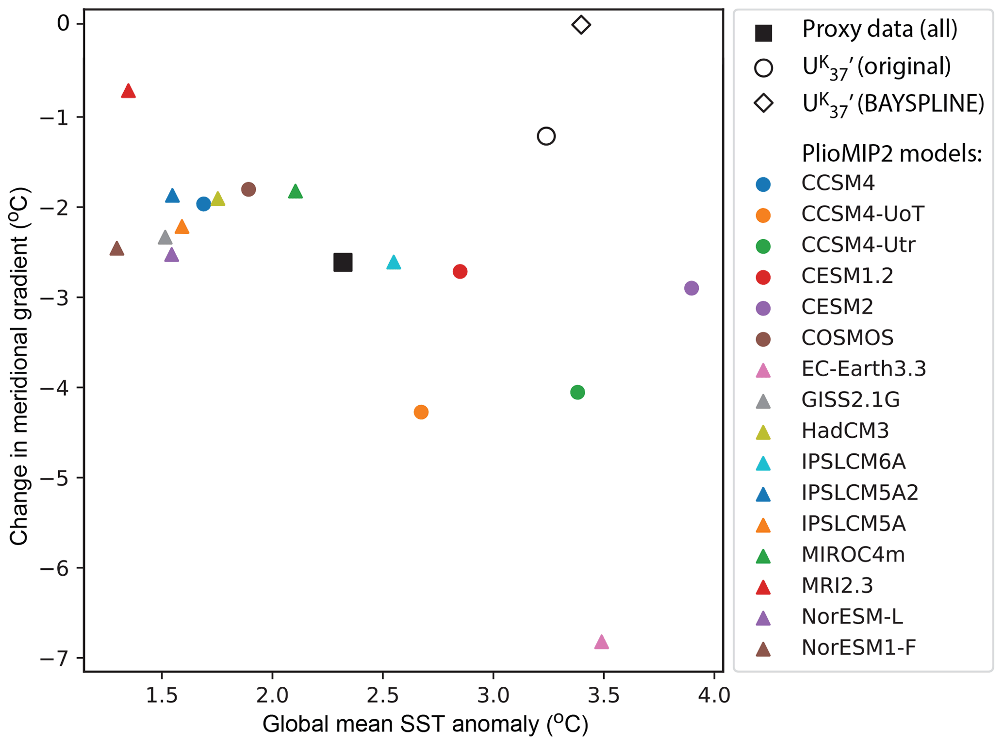
Figure 3 Comparison of KM5c SST data relative to the pre-industrial period (NOAA-ERSST5) for global mean SST anomalies (SSTA) and the change in meridional SST gradient, constructed using proxy data and the suite of PlioMIP2 models. Details of the model experiments are outlined in Table 1 of Haywood et al. (2020). The meridional SST gradient is calculated as 30^∘ S–30^∘ N minus 60–75^∘ N, so that a more negative change in the gradient reflects a larger warming anomaly at high latitudes relative to low latitudes. As we only had data points poleward of 65^∘ N in the Atlantic Ocean, the high-latitude region for both proxy and model gradient calculations focuses on the longitudinal window from 70^∘ W to 5^∘ E. Proxy data calculations were made using either all proxy data (${\mathrm{U}}_{\mathrm{37}}^{{\mathrm{K}}^{\prime }}$ and Mg∕Ca using their original calibrations) or using only ${\mathrm{U}}_{\mathrm{37}}^{{\mathrm{K}}^{\prime }}$ data and comparing the original and BAYSPLINE calibrations. No Mg∕Ca data are available >60^∘ N, so we were unable to calculate Mg∕Ca-only gradients (Fig. 4). The impact of changing the low- and high-latitude bands is explored in Table 1.

Overall, the proxy data show the lowest temperature anomalies in the low latitudes, regardless of proxy (from +3 to −4 ^∘C for sites <30^∘ N/S). A larger range of temperature anomalies is reconstructed in the mid-latitudes and high latitudes (from +9 to −2 ^∘C for sites >30^∘ N/S) (Fig. 4). Thus, there is a broad, but complex, pattern of enhanced warming at the mid-latitudes and high latitudes, reflecting a combination of regional influences on circulation patterns and, to some extent, proxy choice. This pattern is not explained by temporal variability nor sample density within the KM5c time interval: regardless of sample number per site, the standard deviation at any site within the KM5c time bin is <1.5 ^∘C (Fig. S4 in the Supplement). We note that of the 32 sites examined here, 7 provided a single data point for the KM5c interval (Fig. S2, alkenones: ODP Sites 907, 1081, U1337, U1417; Fig. S3, foraminifera Mg∕Ca: DSDP sites 214, 709, 763); the sites are geographically well distributed, however, and so unlikely to significantly impact our global mean/gradient calculations.

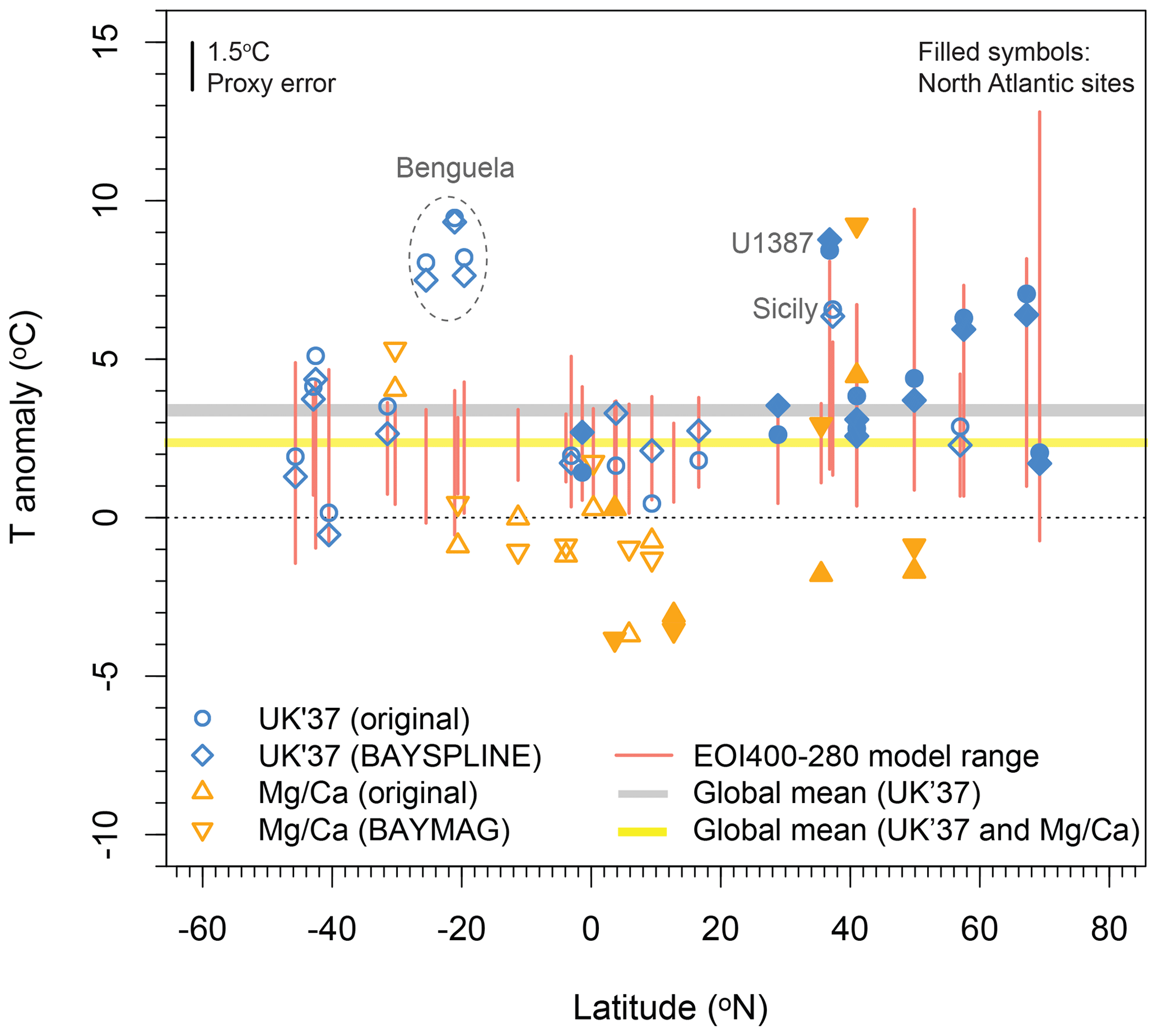
Figure 4 Reconstructed and modelled SST anomalies plotted by latitude. SST reconstructions using the original published data and two Bayesian approaches (BAYSPLINE, BAYMAG) are shown. The anomalies are calculated with reference to the NOAA-ERSST5 data for the years 1870–1899 CE at each site. Vertical red lines show the range of modelled annual SSTs from all PlioMIP2 experiments (Haywood et al., 2020) calculated at the grid boxes containing each site.

Calibration choice has a small impact over the reconstructed patterns of KM5c SST anomalies (Figs. 4, S2, and S3). Below 24 ^∘C, absolute ${\mathrm{U}}_{\mathrm{37}}^{{\mathrm{K}}^{\prime }}$ SSTs using Müller98 are <1 ^∘C lower than those using BAYSPLINE. At high temperatures the non-linearity in the BAYSPLINE calibration means that BAYSPLINE SSTs can be up to $\mathrm{1.67}{}^{\circ }\mathrm{C}\pm \mathrm{0.01}{}^{\circ }\mathrm{C}$ higher than when using Müller98 (Fig. S2). The low-latitude offset between Müller98 and BAYSPLINE has two effects: it elevates the global mean SST (Fig. 3, Table 1) and increases the KM5c meridional SST gradient towards pre-industrial values (Figs. 3 and 4, Table 1). The calibration offsets are less systematic for Mg∕Ca. There is a wider range of offsets between BAYMAG and published SST values (from −4 to +5 ^∘C; Fig. S3, Table S3), although the smallest KM5c SST anomalies continue to be reconstructed in the low latitudes, regardless of which Mg∕Ca calibration is applied (Fig. 4).

Overall, the ${\mathrm{U}}_{\mathrm{37}}^{{\mathrm{K}}^{\prime }}$–temperature anomalies lie within the range given by PlioMIP2 models (Fig. 4). The Mg∕Ca estimates are mainly from the low latitudes, and high-latitude (>60^∘ N/S) Mg∕Ca SST data are not available to calculate meridional gradients using foraminifera data alone (Fig. 4). Mg∕Ca-SST anomalies are generally lower than for ${\mathrm{U}}_{\mathrm{37}}^{{\mathrm{K}}^{\prime }}$, and a cooler KM5c than the pre-industrial period is consistently (but not always) recorded in the low latitudes by Mg∕Ca regardless of calibration choice (Fig. 4). As a result, combining ${\mathrm{U}}_{\mathrm{37}}^{{\mathrm{K}}^{\prime }}$ and Mg∕Ca data leads to a cooler global mean SST (∼2.3 ^∘C) than when using ${\mathrm{U}}_{\mathrm{37}}^{{\mathrm{K}}^{\prime }}$ alone (∼3.2 ^∘C with Müller98, ∼3.4 ^∘C with BAYSPLINE; Fig. 3 and Table 1). At eight sites, the negative KM5c SST anomalies in Mg∕Ca disagree with both the ${\mathrm{U}}_{\mathrm{37}}^{{\mathrm{K}}^{\prime }}$ data and the PlioMIP2 model outputs (Fig. 4). The disagreement is present regardless of whether the Müller98 or BAYSPLINE calibrations are applied, but the difference is larger in the low latitudes for BAYSPLINE because here this calibration generates higher SST values (Sect. 2.3.1). Only three sites have both ${\mathrm{U}}_{\mathrm{37}}^{{\mathrm{K}}^{\prime }}$ and Mg∕Ca data (DSDP Site 609, IODP sites U1313 and U1143) to enable direct comparison between Mg∕Ca and alkenone SST data. Reconstructed SSTs for IODP sites U1313 and U1143 are within calibration uncertainty. At Site U1313 (41^∘ N) there is overlap between both alkenone outputs (Müller98 21.6 ^∘C, BAYSPLINE 20.9 ^∘C) and the original Mg∕Ca reconstruction (22.2 ^∘C), whereas BAYMAG generates warmer SSTs (27.0 ^∘C). At Site 1143 (9^∘ N), BAYSPLINE SSTs are warmer (30.6 ^∘C) than from the Müller98 (28.9 ^∘C), original Mg∕Ca (27.7 ^∘C), and BAYMAG (27.1 ^∘C) calibrations. In contrast, DSDP Site 609 (49^∘ N) has colder Mg∕Ca estimates (original 11.7 ^∘C, BAYMAG 12.5 ^∘C) than alkenones (Müller98 17.7 ^∘C, BAYSPLINE 17.1 ^∘C) or models (Fig. 4).

4 Discussion

4.1 SST expression of the KM5c interglacial

KM5c is characterised by a surface ocean which is ∼2.3 ^∘C (alkenones and Mg∕Ca), ∼3.2 ^∘C (alkenones-only, Müller98 calibration), or ∼3.4 ^∘C (alkenones-only, BAYSPLINE calibration) warmer than pre-industrial values, with a ∼2.6 ^∘C reduction in the meridional SST gradient. The global mean SST anomaly is higher than the 1.7 ^∘C previously calculated for the wider mid-Piacenzian warm period (3.1–3.3 Ma), regardless of proxy choice (IPCC, 2014b). Previous analysis of a suite of models suggested that a climate state resembling the mid-Piacenzian was likely to develop and be sustained under RCP4.5 (Burke et al., 2018). The PlioMIP2 ensemble (Haywood et al., 2020) indicates that best estimates for mid-Piacenzian warming in surface air temperatures (1.7–5.2^∘) are comparable to projections for the RCP4.5 to 8.5 scenarios by 2100 CE ($\text{RCP4.5}=\mathrm{1.8}\pm \mathrm{0.5}$^∘, $\text{RCP8.5}=\mathrm{3.7}\pm \mathrm{0.7}$ ^∘C; IPCC, 2013). Our proxy-based mean global SST anomaly is larger than in most PlioMIP2 models when we use only alkenones or alkenones and Mg∕Ca combined (Fig. 3), and hence our results suggest that the global annual surface air temperature anomaly for KM5c would exceed the PlioMIP2 multi-model surface air temperature mean of 2.8 ^∘C (Haywood et al., 2020). The higher global SST mean recorded in the KM5c proxy data, compared to the PlioMIP2 models, occurs despite the available atmospheric CO₂ reconstructions indicating values below the ∼400 ppmv used in the PlioMIP2 models (Fig. 1). Our synthesis of SST data thus indicates that with atmospheric CO₂ concentrations ≤400 ppmv (comparable to RCP4.5), the surface ocean warming response will likely be larger than indicated in models. Further work is required to increase the temporal resolution of the atmospheric CO₂ reconstructions through KM5c, to improve our understanding of the reconstructed SST response to CO₂ forcing, including whether (or by how much) the reconstructed atmospheric CO₂ differs from model boundary conditions and whether other changes in the model boundary conditions also influence SST patterns (e.g. gateway changes outlined in Sect. 2.4).

Proxy choice, calibration choice, and site selection have all had an impact on the magnitude of the change in meridional SST gradient for KM5c compared to the pre-industrial period (Table 1). Focussing only on a Northern Hemisphere SST gradient leads to higher gradient anomalies than when all of the low latitudes are included (30^∘ S–30^∘ N) because it excludes the high SST anomalies of the Benguela upwelling sites (20–25^∘ S; discussed below, Fig. 4). Smaller meridional SST gradient anomalies occur using BAYSPLINE (+0.03 to −1.66 ^∘C) than the Müller98 calibration for ${\mathrm{U}}_{\mathrm{37}}^{{\mathrm{K}}^{\prime }}$ (−1.18 to −3.00 ^∘C; Table 1), due to the increased low-latitude SST anomalies generated by BAYSPLINE (Fig. 4). Due to several (but not all) low-latitude sites recording negative SST anomalies for KM5c using foraminifera Mg∕Ca, the inclusion of Mg∕Ca data leads to a larger difference in the meridional SST gradient relative to the pre-industrial period (−2.19 to −4.08 ^∘C). Further work is required to fully understand the negative KM5c SST anomalies in some of the low-latitude sites (discussed further below), given their impact on the meridional SST gradients. However, a robust pattern emerging from the data is that the KM5c proxy data detail smaller low-latitude SST anomalies than those of the mid- and high-latitude SST anomalies (Fig. 4), leading to a reduction in the meridional SST gradient relative to the pre-industrial period. Enhanced mid- and high-latitude warming has been observed in other warm intervals of the geological past, including the last interglacial and the Eocene (Evans et al., 2018; Fischer et al., 2018), and is a feature of future climate under elevated CO₂ concentrations (IPCC, 2014a).

There is complexity in the amplitude of the KM5c SST anomaly by latitude and basin, which may reflect patterns of surface ocean circulation. In the Northern Hemisphere, relatively muted warming in the East Greenland Current (ODP Site 907, 69^∘ N) may reflect the presence of at least seasonal sea-ice cover from ca. 4.5 Ma (Clotten et al., 2018). In contrast, relatively high SST anomalies at ODP Sites 642 (67^∘ N) and 982 (58^∘ N) track the northward flow of the North Atlantic Current, accounting for the enhanced warming relative to north-east Pacific IODP Site U1417 (57^∘ N; Figs. 4 and 5). The large North Atlantic SST anomalies also contribute to an enhanced Northern Hemisphere meridional SST gradient of up to 4 ^∘C (>60^∘ N minus 0–30^∘ N; Table 1). For the Southern Hemisphere, a signal of polar amplification is less clearly identified than for the Northern Hemisphere (Fig. 4), although we recognise that all sites are <46^∘ S. Low KM5c SST anomalies (<2 ^∘C) at DSDP sites 593 and 594 (41 and 46^∘ S, respectively) might be accounted for by a similar positioning of the Subtropical Front close to New Zealand during KM5c as today (McClymont et al., 2016; Caballero-Gill et al., 2019). Antarctic Intermediate Water (AAIW) temperatures were also only ∼2.5 ^∘C warmer than pre-industrial values during KM5c, suggesting a small warming in subantarctic waters where AAIW forms (McClymont et al., 2016). In contrast, large anomalies at ODP Sites 1125 (43^∘ S, Pacific) and 1090 (43^∘ S, Atlantic) reflect a greater sensitivity to expanded subtropical gyres during KM5c, contrasting with the Pleistocene equatorward displacement (and enhanced cooling) of subpolar water masses (e.g. Martinez-Garcia et al., 2010) which today places both of these sites poleward of the Subtropical Front.

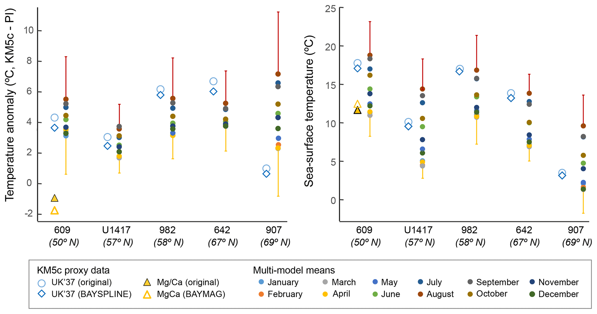
Figure 5 Investigating the potential seasonal signature recorded at high-latitude Northern Hemisphere sites (>50^∘ N), ordered by increasing latitude from left to right. Note that Site U1417 is from the North Pacific, where BAYSPLINE explicitly assumes that a summer signal is recorded >48^∘ N. All other sites are from the Atlantic Ocean/Nordic Seas, where BAYSPLINE assumes an autumn signal >45^∘ N. The original calibration by Müller et al. (1998) proposes that mean annual SSTs are recorded. Standard deviations of the multi-model means are shown for August (red) and April (yellow), which tend to be the maxima and minima, respectively.

Given that our proxy data meridional SST gradient calculations use only two sites to calculate the high-latitude SSTs (ODP Sites 907 and 642), which are also both from the Nordic Seas (Fig. 2), we explored the impact of expanding our high-latitude band into the mid-latitudes. We also explored narrowing the low-latitude band so that it does not include the Benguela upwelling sites, which have a significant data–model offset (Fig. 4) and may be influenced by localised circulation changes (see Sect. 4.2). Previous calculations of Pliocene meridional SST gradients have also considered differences between the mid-latitudes and low latitudes through time (Fedorov et al., 2015). Despite adding four more sites by expanding the high-latitude band to 45^∘ N/S, the meridional SST gradients are reduced by <0.4 ^∘C, from −1.18 to −1.56 ^∘C using the original ${\mathrm{U}}_{\mathrm{37}}^{{\mathrm{K}}^{\prime }}$ data (Table 1). However, it is clear from the distribution of sites (Fig. 2) that our reconstructed KM5c SSTs (and thus the global mean and meridional gradients) have a strong signal from the Atlantic Ocean. There is a relative scarcity of sites from the Indian Ocean, Pacific Ocean, and Southern Ocean, but it is difficult to ascertain what impact this may have had on our global analysis. Further work is required to increase the spatial density of SST data for KM5c and the wider mid-Piacenzian stage, to better evaluate the magnitude of the warming and gradient changes outlined here.

4.2 Proxy data–model comparisons for mid- and high-latitude sites

For the mid-latitudes and high latitudes, we find broad proxy data–model agreements for most sites. In the North Atlantic Ocean, reconstructed SST KM5c anomalies from ${\mathrm{U}}_{\mathrm{37}}^{{\mathrm{K}}^{\prime }}$ fall within the ranges provided by the PlioMIP2 models (Fig. 4) for all but one site (IODP Site U1387, 37^∘ N). The overall ${\mathrm{U}}_{\mathrm{37}}^{{\mathrm{K}}^{\prime }}$–model agreement for the North Atlantic Ocean suggests that, as proposed by Haywood et al. (2013), a focus on a specific interglacial within the mid-Piacenzian provides an improved comparison to the climate being simulated by the PlioMIP2 models. Thus, some of the data–model mismatch in previous mid-Piacenzian syntheses (e.g. Dowsett et al., 2012) may have been due to the averaging of warm peaks which may not have been synchronous in time between sites and/or with the interval being modelled. Disagreements occur between proxies (North Atlantic Ocean) and between proxies and models (Benguela upwelling, Gulf of Cadiz, Mediterranean Sea) (Fig. 4). Here, we explore the potential causes for these offsets in turn.

The largely ${\mathrm{U}}_{\mathrm{37}}^{{\mathrm{K}}^{\prime }}$-derived data from the North Atlantic Ocean tend to align with the warmest model outputs (Fig. 4), and the ${\mathrm{U}}_{\mathrm{37}}^{{\mathrm{K}}^{\prime }}$-SST anomalies also tend to be larger than those from Mg∕Ca. A challenge for understanding the cause(s) of the ${\mathrm{U}}_{\mathrm{37}}^{{\mathrm{K}}^{\prime }}-\mathrm{Mg}/\mathrm{Ca}$ differences is that only two sites have data from both proxies, and these do not show a consistent signal. There is good correspondence between ${\mathrm{U}}_{\mathrm{37}}^{{\mathrm{K}}^{\prime }}$ and the original published Mg∕Ca SSTs for IODP Site U1313 (41^∘ N), whereas at ODP Site 609 Mg∕Ca SSTs (both calibrations) are between 4.6 and 6.1 ^∘C cooler than ${\mathrm{U}}_{\mathrm{37}}^{{\mathrm{K}}^{\prime }}$. It has also been shown that the ${\mathrm{U}}_{\mathrm{37}}^{{\mathrm{K}}^{\prime }}-\mathrm{Mg}/\mathrm{Ca}$ SST offset at Site 609 is not constant with time for the late Pliocene (Lawrence and Woodard, 2017). When using BAYMAG, warmer KM5c SSTs are reconstructed than the original published data at DSDP Site 603 and IODP Site U1313 (35 and 41^∘ N; Fig. 4), but BAYMAG reconstructs SSTs only 0.8 ^∘C warmer than the original published SSTs at Site 609. These mid-latitude North Atlantic Mg∕Ca data are provided by G. bulloides, which may calcify at depth in the water column (e.g. Mortyn and Charles, 2003; Schiebel et al., 1997) and account for those sites where Mg∕Ca reconstructions give lower reconstructed SSTs than from ${\mathrm{U}}_{\mathrm{37}}^{{\mathrm{K}}^{\prime }}$ (Bolton et al., 2018; De Schepper et al., 2013). Alternatively, an offset between alkenones and Mg∕Ca might be accounted for if there is a seasonal bias to the ${\mathrm{U}}_{\mathrm{37}}^{{\mathrm{K}}^{\prime }}$ calibration (e.g. Conte et al., 2006; Schneider et al., 2010). Despite documented seasonality in alkenone production at high latitudes, it has been proposed that mean annual SSTs continue to be recorded by ${\mathrm{U}}_{\mathrm{37}}^{{\mathrm{K}}^{\prime }}$ in sediments (Rosell-Melé and Prahl, 2013), as indicated by the original ${\mathrm{U}}_{\mathrm{37}}^{{\mathrm{K}}^{\prime }}$ calibration (Müller et al., 1998). In contrast, BAYSPLINE explicitly assumes an autumn signal is recorded at Atlantic sites >45^∘ N (Tierney and Tingley, 2018). Despite these differences in interpretation, BAYSPLINE values for KM5c are <0.7 ^∘C cooler than the original published ${\mathrm{U}}_{\mathrm{37}}^{{\mathrm{K}}^{\prime }}$ data (Fig. S2). Although the North Atlantic ${\mathrm{U}}_{\mathrm{37}}^{{\mathrm{K}}^{\prime }}$ data align with a range of mean annual SST anomalies generated by the PlioMIP2 models (Fig. 4), three of the sites show alignment between ${\mathrm{U}}_{\mathrm{37}}^{{\mathrm{K}}^{\prime }}$ SSTs and the July–November values from the multi-model means (Fig. 5). In contrast, Site 907 aligns with cool spring temperatures in the models, perhaps reflecting production after sea ice melt.

The large data–model discrepancy at 30^∘ S reflects three sites which today sit beneath the Benguela upwelling system in the south-east Atlantic (20–26^∘ S; Fig. 4). Part of the data–model discrepancy in the KM5c anomaly can be attributed to the models overestimating pre-industrial SSTs at the northern Benguela sites (NOAA-ERSST5 SSTs are 2–5 ^∘C below the pre-industrial model range) and suggests that models are not fully capturing the local dynamics of the coastal upwelling today (Small et al., 2015). Realistic representations of the Benguela upwelling system today are proposed to require realistic wind stress curl and high-resolution atmosphere and ocean models (<1^∘; Small et al., 2015). Most of the PlioMIP2 simulations use lower-resolution atmosphere and ocean models (Haywood et al., 2020). An increased density of proxy data reconstructing KM5c atmospheric circulation, as well as the application of high-resolution models, may help to understand the observed KM5c data–model discrepancy. Furthermore, there was a deep thermocline during the Pliocene (as reconstructed in the equatorial Pacific (Ford and Ravelo, 2019; Ford et al., 2015; Steph et al., 2006; Steph et al., 2010) and theorised globally (Philander and Fedorov, 2003)), so that warmer subsurface waters than today were upwelled, enhancing local warming. However, warming of ∼3.4 ^∘C in subsurface waters (Ford and Ravelo, 2019) and ∼2.5 ^∘C in intermediate waters (McClymont et al., 2016) for Pliocene interglacials suggests that Pliocene upwelling of warmer waters is unable to fully account for the 7–10 ^∘C SST anomalies at Benguela sites for KM5c. Changes to the distribution of export productivity and SSTs indicate that an overall poleward displacement of the Benguela upwelling system occurred during the Pliocene, so that the main zone of upwelling likely sat close to ODP Site 1087 at 31^∘ S (Etourneau et al., 2009; Petrick et al., 2018; Rosell-Melé et al., 2014). As the northern and southern Benguela regions are today marked by differences in the seasonality of the upwelling, a temporal shift in upwelling intensity may also account for some of the large SST anomaly (Haywood et al., 2020). Thus, the data–model disagreement may be accounted for by a combination of displaced upwelling and warmer upwelled waters, giving large SST anomalies in Benguela proxy data, alongside the challenges of modelling both the pre-industrial and KM5c upwelling system and its associated SSTs.

Data–model disagreement also occurs at two Northern Hemisphere sites where ${\mathrm{U}}_{\mathrm{37}}^{{\mathrm{K}}^{\prime }}$-SST anomalies exceed those given by the range of model predictions (Fig. 4). Punto Piccola (Sicily, 37^∘ N) is located within the Mediterranean Sea, whereas IODP Site U1387 (37^∘ N, Iberian margin) records the influence of the waters sourced from the Azores Current and the subtropical gyre. The data–model disagreement for KM5c reflects warmer SST estimates from the proxy data compared to the models, despite the good agreement for the pre-industrial period suggesting that locally complex ocean circulation in these near-shore and marginal marine settings may have been captured in the models. For Punto Piccola, the data–model offset is also likely to be a minimum because BAYSPLINE Mediterranean SSTs explicitly record November–May temperatures (Tierney and Tingley, 2018), and alkenone production below the sea surface has also been proposed (Ternois et al., 1997): both scenarios would act to raise mean annual SSTs further from those simulated in the PlioMIP2 models (Fig. 4). Further multi-proxy investigation is required to identify whether the data–model disagreements in the Benguela upwelling, Gulf of Cadiz, and Mediterranean Sea reflect challenges in modelling near-shore or complex oceanographic systems and/or biases in the temperature signal recorded by the proxy data.

4.3 Data–model comparisons for low-latitude sites

The low-latitude ${\mathrm{U}}_{\mathrm{37}}^{{\mathrm{K}}^{\prime }}$-SST anomalies for KM5c align well with the PlioMIP2 models (Fig. 4). At ODP Sites 806 and 959, the Mg∕Ca anomalies using the original calibrations are both +0.3 ^∘C compared to the pre-industrial period (Fig. 4) and also align with the PlioMIP2 models. At Site 806 the BAYMAG KM5c anomaly (+1.7 ^∘C) also aligns with the PlioMIP2 models. Only one low-latitude site has both ${\mathrm{U}}_{\mathrm{37}}^{{\mathrm{K}}^{\prime }}$ and Mg∕Ca SST data: ODP Site 1143 (9^∘ N) records KM5c anomalies of +0.8 to +2.5 ^∘C (${\mathrm{U}}_{\mathrm{37}}^{{\mathrm{K}}^{\prime }}$) or −0.7 to −1.3 ^∘C (Mg∕Ca). Although the ${\mathrm{U}}_{\mathrm{37}}^{{\mathrm{K}}^{\prime }}$ data align with the model outputs for Site 1143, the negative anomaly in Mg∕Ca lies outside the model range for mean annual SST (Fig. 4).

Six of the low-latitude sites have negative low-latitude SST anomalies in KM5c from foraminifera Mg∕Ca; these occur regardless of whether the original or BAYMAG calibrations are applied and for both G. ruber and T. sacculifer-based reconstructions. The negative KM5c Mg∕Ca-SST anomalies lie beyond those shown across the PlioMIP2 model range (Fig. 4), despite the absolute Mg∕Ca SSTs reconstructed from these sites for KM5c falling within the model range for all but two of the sites (ODP Sites 999 (13^∘ N) and 1241 (6^∘ N); Fig. S5). However, the absolute SST values reconstructed for KM5c from Mg∕Ca tend to align with the colder model outputs (Fig. S5).

Mg∕Ca-SST calibration choice has no consistent impact on the KM5c anomalies (across all latitudes; Fig. 4). Therefore, the corrections for secular seawater Mg∕Ca change and/or non-thermal influences over Mg∕Ca, which are accounted for in BAYMAG (Tierney et al., 2019b), do not account for these cold tropical KM5c anomalies. For example, for ODP Site 806 in the western Pacific warm pool, BAYMAG SST estimates for KM5c are ∼1 ^∘C warmer than the published Mg∕Ca record (Wara et al., 2005). For Site 999 in the Caribbean Sea, BAYMAG SST estimates for KM5c are ∼0.5 ^∘C cooler than the published Mg∕Ca record (De Schepper et al., 2013). This also suggests that the impact of Mg∕Ca_seawater change on SST is small on warm pool sites. The Mg∕Ca_seawater correction used in BAYMAG is conservative, drawing on multiple lines of physical evidence (corals, fluid inclusions, calcite veins, etc.) (Tierney et al., 2019b). Given the variable directions of the offsets between published and BAYMAG SSTs shown here, the Mg∕Ca_seawater correction is unable to account for the data–model offsets observed for the low latitudes.

CaCO₃ dissolution in the water column and sediments could lead to a cool bias on the Mg∕Ca SSTs (Dekens et al., 2002; Regenberg et al., 2006, 2009). However, the cool KM5c anomalies also occur if the forward-modelled core-top Mg∕Ca SSTs from BAYMAG are used as the pre-industrial “reference” (Fig. S6). The cold low-latitude anomalies for KM5c could reflect an increase in the calcification depth of the foraminifera, since the surface-dwelling foraminifera analysed here calcify at a range of depths, particularly in the tropics where the thermocline is deep in comparison to mid-latitudes to high latitudes (Fairbanks et al., 1982; Curry et al., 1983). The negative anomalies are broadly smaller for G. ruber (−0.4 to −1.2 ^∘C) than for T. sacculifer (−0.6 to −3.5 ^∘C), consistent with a deeper depth habitat for the latter (Curry et al., 1983), although at Site 959 the G. ruber anomaly using BAYMAG is −3.8 ^∘C. There is therefore a lack of consistency between sites, which is difficult to resolve when single species have been analysed for each of the sites through KM5c.

Where there are very large differences between BAYMAG and published Mg∕Ca SST estimates, regardless of latitude (e.g. North Atlantic; Fig. 4), we suggest that some combination of calibration difference, Mg∕Ca_seawater change, and/or other environmental factors including seasonality and calcification depth may offer an explanation. To fully investigate the cause(s) of offsets in Mg∕Ca SST reconstructions requires future multi-species analysis for Mg∕Ca for each site and multi-proxy analysis for each site. Such an approach would enable the exploration of a wider range of potential influences over both the Mg∕Ca and ${\mathrm{U}}_{\mathrm{37}}^{{\mathrm{K}}^{\prime }}$-SST reconstructions and a reduction in the uncertainties of the reconstructed SSTs and their anomalies. Alongside foraminifera Mg∕Ca and ${\mathrm{U}}_{\mathrm{37}}^{{\mathrm{K}}^{\prime }}$ analyses, additional proxies which are likely to add valuable information about water column structure and seasonality could include TEX₈₆ (Schouten et al., 2002), long-chain diols (Rampen et al., 2012), and clumped isotopes (Tripati et al., 2010). Previous research has demonstrated that even within a single site there can be offsets between proxies which are not continuous through time (e.g. Lawrence and Woodard, 2017; Petrick et al., 2018), so that high-resolution and multi-proxy work is required to fully understand the offsets we have identified here. Resolving the causes of the different proxy–proxy and proxy–model offsets is important because they impact the calculation of the global mean SST anomaly relative to pre-industrial values; however, even with the inclusion of the overall cooler Mg∕Ca data, the combined KM5c proxy data still indicate a global mean SST anomaly which is larger than most models from the PlioMIP2 experiments (Fig. 3).

5 Conclusions

This study has generated a new multi-proxy synthesis of SST data for an interglacial stage (KM5c) from the Pliocene. By selecting an individual interglacial, with orbital forcing similar to modern values, we are able to focus on the SST response to atmospheric CO₂ concentrations comparable to today and the near future (∼400 ppmv) but elevated relative to the pre-industrial period. Using strict stratigraphic protocols we selected only those data which could be confidently aligned to KM5c. By comparing different calibrations and two different proxy systems (${\mathrm{U}}_{\mathrm{37}}^{{\mathrm{K}}^{\prime }}$ and Mg∕Ca in planktonic foraminifera) we identified several robust signals which are proxy-independent. First, global mean SSTs during KM5c were warmer than pre-industrial values. Second, there was a reduced meridional SST gradient which is the result of relatively small low-latitude SST anomalies and a larger range of warming anomalies for the mid-latitudes and high latitudes. Overall, there is good data–model agreement for both the absolute SSTs and the anomalies relative to the pre-industrial period, although there are complexities in the results. Further work is required to generate multi-proxy SST data from single sites, accompanied by robust reconstructions of thermocline temperatures using multi-species foraminifera analysis, so that the range of factors explaining proxy and calibration offsets can be explored more fully.

The choice of proxy for SST reconstruction impacts the overall calculation of global mean SST and the meridional gradients. The negative anomalies in Mg∕Ca SSTs at 6 of the 16 low-latitude sites lowers the global mean SST of KM5c from ∼3.2–3.4 ^∘C (${\mathrm{U}}_{\mathrm{37}}^{{\mathrm{K}}^{\prime }}$-only) to ∼2.3 ^∘C (combined ${\mathrm{U}}_{\mathrm{37}}^{{\mathrm{K}}^{\prime }}$ and Mg∕Ca). The meridional SST gradient anomalies are decreased to −2.6 ^∘C (combined ${\mathrm{U}}_{\mathrm{37}}^{{\mathrm{K}}^{\prime }}$ and Mg∕Ca) relative to the pre-industrial period, although a more muted reduction (up to $-\mathrm{1.18}{}^{\circ }$ C) occurs with ${\mathrm{U}}_{\mathrm{37}}^{{\mathrm{K}}^{\prime }}$ alone. A number of factors may lead to a cool bias in the foraminifera Mg∕Ca SSTs, which require further investigation through multi-proxy and multi-species analysis, particularly at low-latitude sites.

We identify the strongest warming across the North Atlantic region. The results are consistent with the PlioMIP2 models, although the largely ${\mathrm{U}}_{\mathrm{37}}^{{\mathrm{K}}^{\prime }}$ data sit at the high end of the calculated model anomalies. Although seasonality may play a role in the proxy data signal, these results also suggest that many models may underestimate high-latitude warming even with the moderate CO₂ increases identified in KM5c relative to the pre-industrial period. More data points are required to fully explore these patterns: for seven sites only one data point lay within KM5c, and more than half of the analysed sites (18/32) recorded Atlantic Ocean SSTs.

Both the PlioMIP2 models (Haywood et al., 2020) and future projections (IPCC, 2019) indicate that warming is higher over land than in the oceans in response to higher atmospheric CO₂ concentrations. Our synthesis of KM5c thus likely represents a minimum warming to be expected with atmospheric CO₂ concentrations of ∼400 ppmv. Even under low-CO₂ emission scenarios, our results demonstrate that surface ocean warming may be expected to exceed model projections and will be accentuated in the higher latitudes.