the Creative Commons Attribution 4.0 License.
the Creative Commons Attribution 4.0 License.
 | 06 Jan 2020
Modeling a modern-like pCO2 warm period (Marine Isotope Stage KM5c) with two versions of an Institut Pierre Simon Laplace atmosphere–ocean coupled general circulation model
Ning Tan
Camille Contoux
Gilles Ramstein
Christophe Dumas
Pierre Sepulchre
Zhengtang Guo
The mid-Piacenzian warm period (3.264 to 3.025 Ma) is the most recent geological period with present-like atmospheric pCO2 and is thus expected to have exhibited a warm climate similar to or warmer than the present day. On the basis of understanding that has been gathered on the climate variability of this interval, a specific interglacial (Marine Isotope Stage KM5c, MIS KM5c; 3.205 Ma) has been selected for the Pliocene Model Intercomparison Project phase 2 (PlioMIP 2). We carried out a series of experiments according to the design of PlioMIP2 with two versions of the Institut Pierre Simon Laplace (IPSL) atmosphere–ocean coupled general circulation model (AOGCM): IPSL-CM5A and IPSL-CM5A2. Compared to the PlioMIP 1 experiment, run with IPSL-CM5A, our results show that the simulated MIS KM5c climate presents enhanced warming in mid- to high latitudes, especially over oceanic regions. This warming can be largely attributed to the enhanced Atlantic Meridional Overturning Circulation caused by the high-latitude seaway changes. The sensitivity experiments, conducted with IPSL-CM5A2, show that besides the increased pCO2, both modified orography and reduced ice sheets contribute substantially to mid- to high latitude warming in MIS KM5c. When considering the pCO2 uncertainties (50 ppmv) during the Pliocene, the response of the modeled mean annual surface air temperature to changes to pCO2 ( ppmv) is not symmetric, which is likely due to the nonlinear response of the cryosphere (snow cover and sea ice extent). By analyzing the Greenland Ice Sheet surface mass balance, we also demonstrate its vulnerability under both MIS KM5c and modern warm climate.
- Article
(11967 KB) - Full-text XML
-
Supplement
(778 KB) - BibTeX
- EndNote


The mid-Piacenzian warm period (MPWP; 3.264 to 3.025 Ma) is the most recent geological period with a present-like pCO2 concentration and exhibited significant warming relative to today. This interval has been intensively studied during the past 3 decades as this time period is generally considered to be a potential analog of the future warmer climate. There is an abundance of marine and terrestrial data that allow us to reconstruct the ocean or land temperatures and soil and vegetation conditions for this period. The reconstructed pCO2 for the MPWP ranges from 350 to 450 ppmv (Bartoli et al., 2011; Pagani et al., 2010; Martínez-Botí et al., 2015), which bracket the present-day level. The MPWP is thought to be globally warmer by 2–4 ∘C than pre-industrial climate (e.g., Dowsett et al., 2009). A large warming amplification of 7–15 ∘C is estimated in Arctic regions derived from terrestrial proxies from Lake El'gygytgyn in NE Arctic Russia (Brigham-Grette et al., 2013) and Ellesmere Island in the Arctic Circle (Rybczynski et al., 2013). The meridional and zonal sea surface temperature (SST) gradients are reduced compared to the present day, but the magnitude of this reduction is uncertain. Some studies demonstrate substantial decreases in both the zonal and meridional SST gradients over the Pacific region during the MPWP (Wara et al., 2005; Ravelo et al., 2006; Fedorov et al., 2013). The largely reduced SST gradients can be explained by a significant reduction in the meridional gradient of cloud albedo (Burls and Fedorov, 2014). However, the most recent study by Tierney et al. (2019) confirms that the reduced magnitude of the SST gradients during the MPWP is moderate when compared to the present condition. This result also agrees with previous studies (Zhang et al., 2014; O'Brien et al., 2014). Reconstruction of vegetation distribution indicates a northward shift of boreal forest at the expense of tundra regions due to the warmer conditions (Salzmann et al., 2008). Associated with this strong warmth, the eustatic sea level is estimated to have been 22 () m higher (between 2.7 and 3.2 Ma) than at present (e.g., Miller et al., 2012) suggesting a complete disintegration of the Greenland Ice Sheet and a significant collapse of the West Antarctic Ice Sheet as well as unstable regions of East Antarctica (Hill, 2009; Dolan et al., 2015; Koenig et al., 2015).
An early motivation for studying this period was to apply the knowledge thus gained to the issue of the ongoing climate change. However, considering the non-equilibrium state of the present and the future climate due to the continuously changing anthropogenic forcing factors, the simulated quasi-equilibrium MPWP may not be directly regarded as an analog of future warming (Crowley, 1991). The importance of studying the MPWP nowadays is to investigate the abilities of climate models to produce warm climates and to study the relative impacts of forcings and feedbacks of internal climate components under warm conditions, which can assist in developing future climate projections. In Pliocene Model Intercomparison Project phase 1 (PlioMIP1), 11 models involved in the MPWP experiments. Among these models, there is agreement with regard to surface temperature change in the tropics but a lack of agreement on temperature changes at high latitudes as well as total precipitation rate in the tropics (Haywood et al., 2013). The modeled Atlantic Meridional Overturning Circulation and the associated ocean heat transport for this interval in models are not very different compared to modern conditions (Zhang et al., 2013). However, when comparing them to proxy data of sea surface and surface air temperature, climate models uniformly underestimate the warming in the high latitudes (Dowsett et al., 2012, 2013; Haywood et al., 2016b). Reasons for this discord between data and model are complex, but they can be attributed to three main aspects: boundary condition uncertainty, modeling uncertainty (e.g., the model bias, annual variability in the produced climatology fields), and data uncertainty (Haywood et al., 2013). In PlioMIP1, the MPWP is regarded simply as a stable interval despite the climate variability existing over a 300 kyr time slab due to the climate sensitivity and orbital parameters changing, thus the boundary conditions are made as an averaged condition over this long interval, whereas proxy data are representative of some orbital conditions inside this time slab. This boundary condition uncertainty is thus considered as the main contributor to this data–model discrepancy (Haywood et al., 2016a). Therefore, the PlioMIP phase 2 (PlioMIP2) switched to choosing a representative interglacial during the MPWP interval: Marine Isotope Stage KM5c (MIS KM5c; 3.205 Ma). Thus, boundary conditions (known as PRISM4; Dowsett et al., 2016) have been updated for PlioMIP2, which include a new paleogeography reconstruction containing ocean bathymetry and land–ice surface topography and which represent the closure of the Bering Strait and north Canadian Arctic Archipelago region and a reduced Greenland Ice Sheet by 50 % in comparison to PlioMIP1. Besides, extra information on lake distribution and soil types (Pound et al., 2014) is also provided but not used in this paper.
This study is conducted within the framework of PlioMIP2. Here we employ the new PRISM4 boundary conditions to conduct the MPWP experiments by using two French atmosphere–ocean general circulation model (AOGCM) models: IPSL-CM5A and the updated IPSL-CM5A2. The purpose of this study is to better understand the warm climate of the MPWP and to study the sensitivity of the IPSL model to changes in boundary conditions, such as changes in the land–sea mask and pCO2. As the IPSL AOGCM model has participated in PlioMIP1 (Contoux et al., 2012), we also compare the modeling results of PlioMIP2 with those of PlioMIP1 to quantify the impact of the high-latitude seaways' changes on the climate system.
To accomplish the modeling work, we have employed the two versions of the Institute Pierre-Simon Laplace (IPSL) AOGCM: IPSL-CM5A and IPSL-CM5A2. IPSL-CM5A is a low-resolution coupled model which has been applied in CMIP5 for historical and future simulations (Dufresne et al., 2013) as well as for Quaternary and Pliocene paleoclimate studies (Kageyama et al., 2013; Contoux et al., 2012). IPSL-CM5A2 (Sepulchre et al., 2020) is an updated version of IPSL-CM5A. Critical changes compared to IPSL-CM5A include (i) technical developments to make IPSL-CM5A2 run faster (64 yr d−1 in CM5A2 instead of 8 yr d−1 in CM5A), (ii) updates of the versions of components and (iii) a major retuning of the cloud radiative forcing to correct the cold bias in the mid- and high latitudes that is known to be present in CM5A. Thus, to compare it with PlioMIP1 results (Contoux et al., 2012), we carried out the PlioMIP2 core experiment with IPSL-CM5A and the PlioMIP2 core experiment and tiered experiments with IPSL-CM5A2 to save the computational cost. The various components of the model are briefly described in the following subsections, and the reader is referred to Dufresne et al. (2013) for details.
2.1 Atmosphere
The atmosphere component is LMDZ (Hourdin et al.,2013) developed at Laboratoire de Météorologie Dynamique (LMD) in France (the Z of LMDZ indicates that this model has the specificity to be zoomed for regional studies). This is a complex model that incorporates several processes decomposed into a dynamic part that calculates the numerical solutions of the general equations of atmospheric dynamics and a physical part, calculating the details of the climate in each grid point and containing parameterizations processes such as the effects of clouds, convection, and orography (LMD Modelling Team, 2014). Atmospheric dynamics are represented by a finite-difference discretization of the primitive equations of motion (e.g., Sadourny and Laval, 1984) on a longitude–latitude Arakawa C-grid (e.g., Kasahara, 1977). The horizontal resolution of the model is 96×95, corresponding to an interval of 3.75∘ in longitude and 1.9∘ in latitude. There are 39 vertical levels, with around 15 levels above 20 km. This model has the specificity to be zoomed (the Z of LMDZ) if necessary on a specific region and then may be used for regional studies (e.g., Contoux et al., 2013). In IPSL-CM5A2, retuning of the model has been done by altering the cloud radiative effect to decrease the cold bias of the model. More details can be found in Sepulchre et al. (2020).
2.2 Land
The land component in both CM5A and CM5A2 is ORCHIDEE (Organizing Carbon and Hydrology In Dynamic Ecosystems; Krinner et al., 2005), which is comprised of three modules: hydrology, vegetation dynamics, and carbon cycle. The hydrological module (Ducoudré et al., 1993) describes the exchange of energy and water between the atmosphere as well as the biospheres and the soil water budget (Krinner et al., 2005). Vegetation dynamics parameterization is derived from the dynamic global vegetation model LPJ (Sitch et al., 2003; Krinner et al., 2005). The carbon cycle model simulates plant phenology and carbon dynamics of the terrestrial biosphere. Vegetation distribution is described using 13 plant functional types (PFTs) including agricultural C3 and C4 plants, which are not present in the MPWP simulations. In this case, hydrology and carbon modules are activated, but vegetation is prescribed as the PlioMIP1 study by Contoux et al. (2012), using 11 PFTs, derived from the PRISM3 vegetation dataset (Salzmann et al., 2008). Therefore, soil, litterfall, and vegetation carbon pools (including leaf mass and thus LAI, leaf area index) are calculated as a function of dynamic carbon allocation.
2.3 Ocean and sea ice
The ocean model included in IPSL-CM5A is NEMOv3.2 (Madec, 2008), which includes three principle modules: OPA (for the dynamics of the ocean), PISCES (for ocean biochemistry), and LIM (for sea ice dynamics and thermodynamics). The configuration of this model is ORCA2.3 (Madec and Imbard, 1996), which uses a tripolar global grid and its associated physics. The average horizontal resolution is 2∘ by 2∘, which increases to 0.5∘ in the tropics, and there are 31 layers in the vertical. Temperature and salinity advection are calculated by a total variance dissipation scheme (Lévy et al., 2001; Cravatte et al., 2007). The mixed layer dynamics are parameterized using the turbulent kinetic energy (TKE) closure scheme of Blanke and Delecluse (1993) improved by Madec (2008). The sea ice module LIM2 is a two-level thermodynamic–dynamic sea ice model (Fichefet and Morales maqueda 1997). Sensible heat storage and vertical heat conduction within snow and ice are determined by a three-layer model. The OASIS coupler (Valcke, 2006) is used to interpolate and exchange the variables and to synchronize the models. This coupling and interpolation procedures ensure local energy and water conservation. The new version NEMOv3.6 is included in IPSL-CM5A2, in which the river runoffs are now added through a non-zero depth and have a specific temperature and salinity. The coupling system has been switched from OASIS3.3 to OASIS3-MCT (MCT standing for model coupling toolkit). More details are provided by Sepulchre et al. (2020).

Figure 1Anomalies of the PlioMIP2 topography relative to PI control (a) and PlioMIP 1 (b).
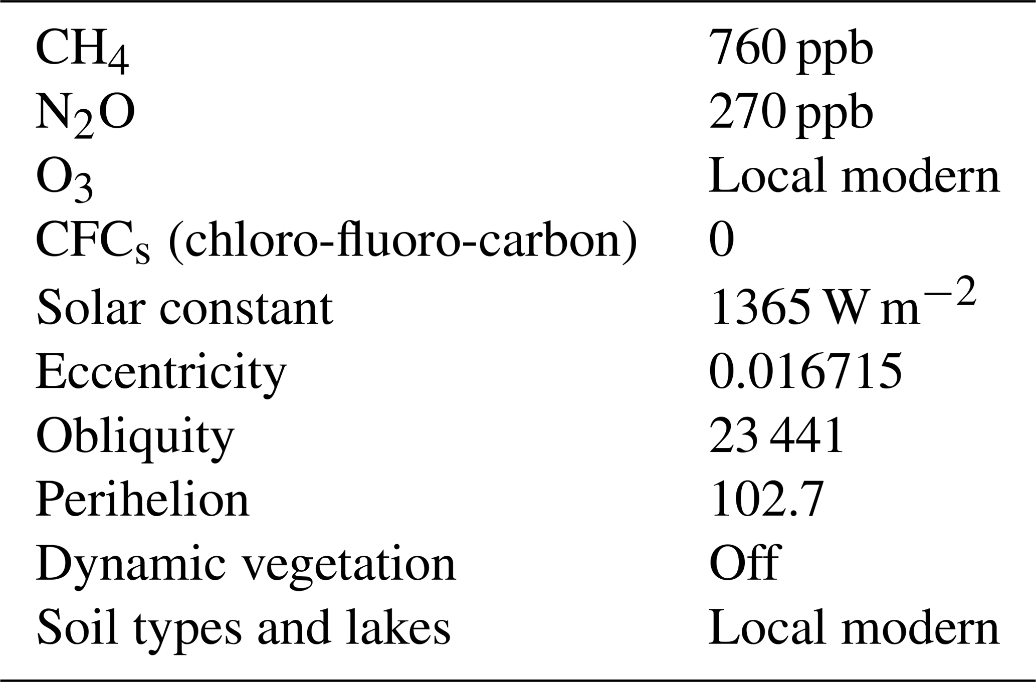
This section describes the boundary and the initial conditions imposed in our experiments. Here, the experiment names are generally consistent with the design of PlioMIP2 (Haywood et al., 2016a), and they are referred to by the abbreviated form E(x)(c), where c is the concentration of atmospheric CO2 in ppmv and x represents boundary conditions that have been changed from the pre-industrial (PI) conditions, such that x can be absent for cases in which no boundary conditions have been modified or it can be “o” for a change in orography and/or “i” for a change in land ice configuration. Because we report on experiments performed with two versions of the IPSL model, we indicate the experiment conducted using the updated version of the model by the suffix “_v2”.
3.1 Pre-industrial experiments
The pre-industrial control simulation in IPSL-CM5A was performed as required by CMIP5/PMIP3 by the LSCE (Le laboratoire des sciences du climat et de l'environnement) modeling group. It is a 2800-year simulation, which already started from equilibrium conditions for the carbon pools (Dufresne et al., 2013). The pre-industrial control simulation in IPSL-CM5A2 was conducted by Sepulchre et al. (2020) and forced by CMIP5 pre-industrial boundary conditions and has a 3000-year integration length.
Table 1Configuration common to all experiments described in this paper.
3.2 Pliocene experiments
We have conducted six AOGCM experiments for PlioMIP2; they are the core experiment Eoi400 using the IPSL-CM5A model and the core experiment Eoi400_v2 as well as four tiered experiments E400_v2, Eoi450_v2, Eoi350_v2, and Eo400_v2 using the IPSL-CM5A2 model. The pCO2 concentration in each experiment is indicated in the experiment name as mentioned above. Other greenhouse gases and orbital forcing are kept the same as in the IPSL PI control run (Table 1). Vegetation is kept the same as in the PlioMIP1 AOGCM simulation by Contoux et al. (2012). Soil patterns and river routing retain the same configurations with PI control, except for the regions where the changes to the topography modify the river routing and the estuaries. The land–sea mask in these experiments is modified from the present only by closing the Bering Strait and the north Canadian Arctic Archipelago region and by modifying the topography in the Hudson Bay (Fig. 1). The ice sheet mask is changed to the PRISM4 dataset (Dowsett et al., 2016) except in the Eo400_v2 experiment, in which the modern ice sheet is imposed. Topography in these five experiments is calculated based on modern topography used in the IPSL model, on which the anomaly between the PRISM4 reconstructed topography and the modern topography provided by the PlioMIP2 database (Haywood et al., 2016a) is superimposed. Wherever the resulting topography was lower than zero, it was replaced by the absolute PRISM4 topography. Figure 1 shows the resulting topography anomalies in our PlioMIP2 experiments compared to PI and PlioMIP1 experiments. The initial sea surface temperature and sea ice in Eoi400 and Eoi400_v2 are derived from the IPSL PlioMIP1 AOGCM simulation (Contoux et al., 2012). Eoi400 has run for 800 modeling years and the initial condition is from the equilibrium state of the PlioMIP1 experiment (Contoux et al., 2012), which has 650 years' integration length. Eoi400_v2 has run for 1500 modeling years. Average climatologies for these two experiments are calculated over the last 50 years. Four tiered experiments (E400_v2, Eoi450_v2, Eoi350_v2, Eo400_v2) are conducted based on the equilibrium state of the Eoi400_v2 core experiment and have 400 years of integration length. Average climatologies for these four experiments are calculated over the last 30 years. The different averaging period lengths for the core experiments (over the last 50 years) and tiered experiments (over the last 30 years) are chosen based on the different experiment running lengths and their final equilibrium states (see the equilibrium analysis in the follow). Table 2 summarizes the aforementioned information. Figure S1 in the Supplement shows time series of surface air temperature and deep ocean temperature at around 2.3 km depth. For both core simulations, the trend in both the global mean surface air temperatures (<0.18 ∘C century−1) and the deep ocean temperature (<0.05 ∘C century−1) over the final 50 years of integration are small. The tiered experiments also show relatively stable trends over the last 30 years of integration (<0.2 ∘C and <0.08 ∘C per century in surface air temperature and subsurface ocean temperature, respectively). Therefore, we conclude that model runs have reached a quasi-equilibrium state.
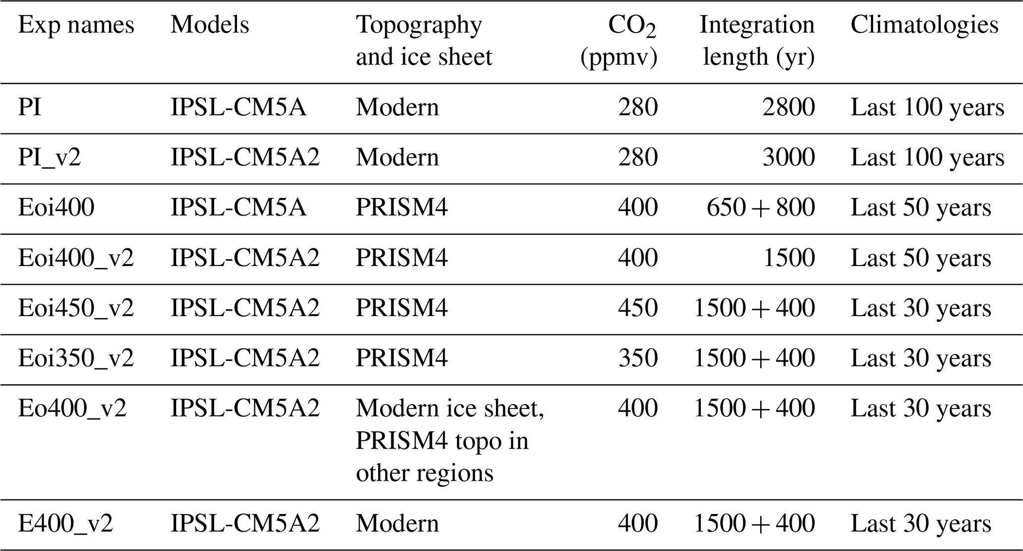
Table 3Diagnostics for each experiment. The anomalies are computed against the PI controls corresponding to the version of the numerical model employed. MA: mean annual; PRECIP: precipitation; SST: sea surface temperature; SSS: sea surface salinity; AMOC: the Atlantic Meridional Overturning Circulation.
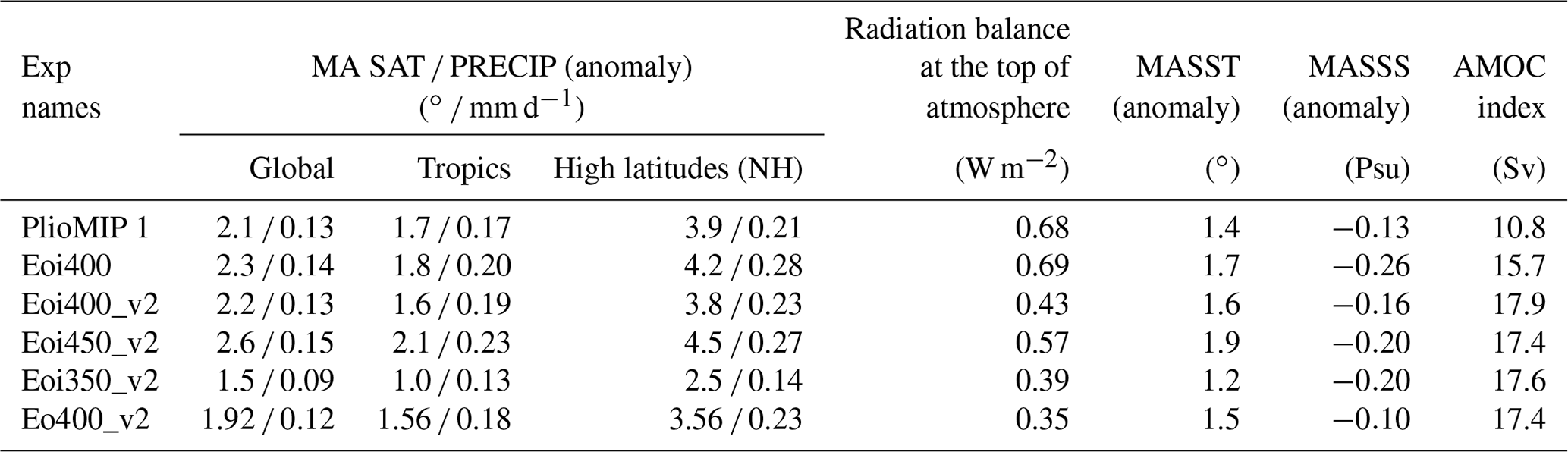

Figure 2Anomalies of mean annual SAT (a, c), mean annual precipitation rates (d, f), and mean annual SST (g, i) for PlioMIP 2 (Eoi400) and PlioMIP 1 conducted with IPSL-CM5A in comparison with the associated pre-industrial control experiment. Panels (b), (e), and (h) represent the zonal mean of related anomalies (red lines for Eoi400, blue lines for PlioMIP 1).
Although a standard pCO2 of 400 ppmv is selected for the Pliocene core experiments, the pCO2 records during this interval mostly range from 350 to 450 ppmv. Thus, the tiered experiments Eoi450_v2 and Eoi350_v2 are conducted to investigate the impact of pCO2 uncertainty on the modeled Pliocene climate. The tiered experiments E400_v2 and Eo400_v2 combined with the core experiment Eoi400_v2 and PI control are used to quantify the relative importance of pCO2, land ice, and orography in the PlioMIP2 warmth. Because of the limited computational resources, we apply the linear decomposition for the forcing factors as d = E400_v2 – E280_v2 (1); dTorography = Eo400_v2 – E400_v2 (2); dTland_ice = Eoi400_v2 – E400_v2 (3); ΔT = d + dTorography + dTland_ice (4).
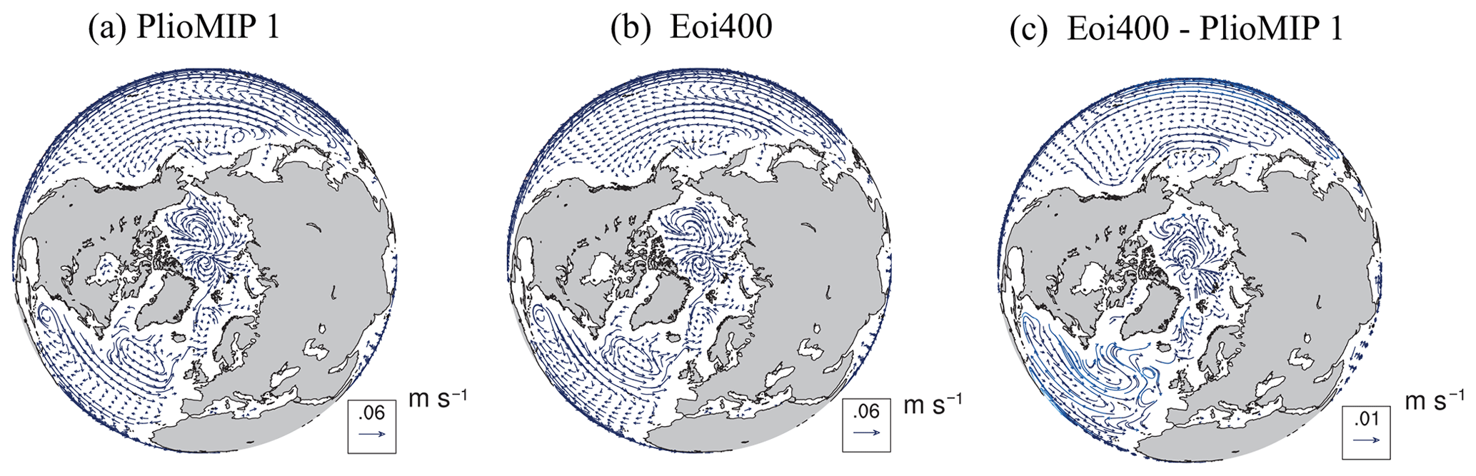
Figure 3Mean annual ocean current above 500 m for PlioMIP 1 (a) and Eoi400 (b); (c) shows the difference in ocean current between Eoi400 and PlioMIP1.
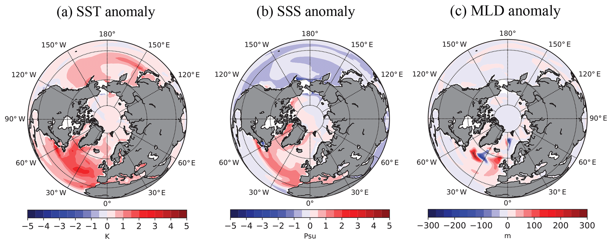
Figure 4The differences in the mean annual sea surface temperature (a), sea surface salinity (b), and the mixed layer depth (c) between Eoi400 and PlioMIP 1.
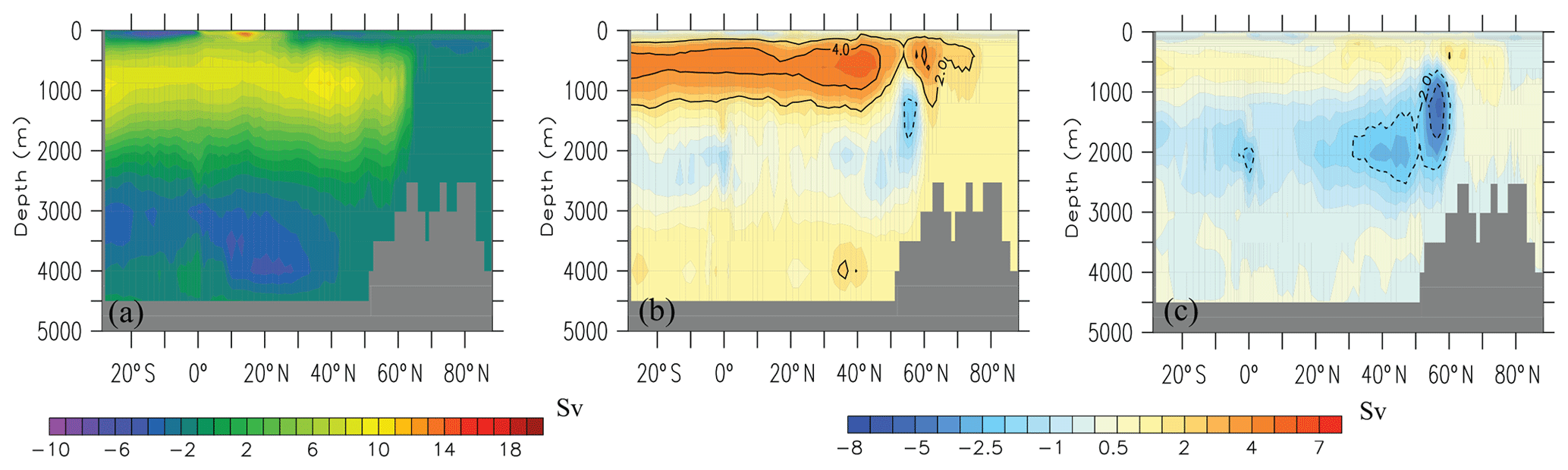
Figure 5Mean annual AMOC of PI control (a) and AMOC anomalies of Eoi400 (b) and PlioMIP 1 (c) in comparison with PI conditions.
4.1 Pliocene runs with IPSL-CM5A
4.1.1 Results in the atmosphere
Figure 2 shows the anomalies of global mean annual near-surface air temperature (SAT; i.e., temperature at 2 m), precipitation rate, and SST between PlioMIP experiments and the pre-industrial control with IPSL-CM5A. The global mean annual SAT in Eoi400 is 14.4 ∘C, which is 2.3 ∘C warmer than that of the pre-industrial one. The warming in Northern Hemisphere (NH) high latitudes ( N) (4.2 ∘C) is higher than that in the tropics (1.8 ∘C). The magnitude of the warming for Eoi400 is slightly larger than that for the PlioMIP1 experiment, which shows a global warming by 2.1 ∘C. The major differences in SAT between Eoi400 and PlioMIP1 are found, respectively, in midlatitude Eurasia and Arctic regions due to the change in regional topography and high-latitude seaways as well as the reduced Greenland Ice Sheet. Thus, Eoi400 shows a reduced meridional temperature gradient than that in the PlioMIP1 experiment.
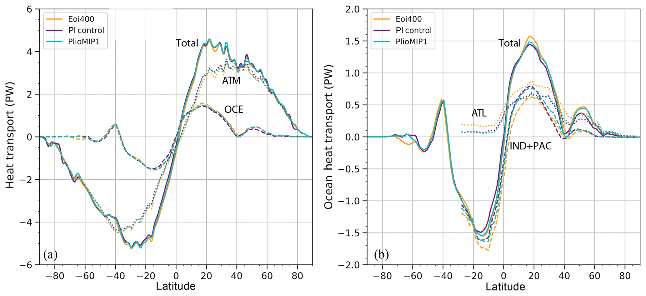
Figure 6Meridional heat transport in both atmosphere and ocean (a); meridional ocean heat transport in different regions (b). (Orange, purple, and blue lines, respectively, represent the results of Eoi400, the PI control, and PlioMIP 1).
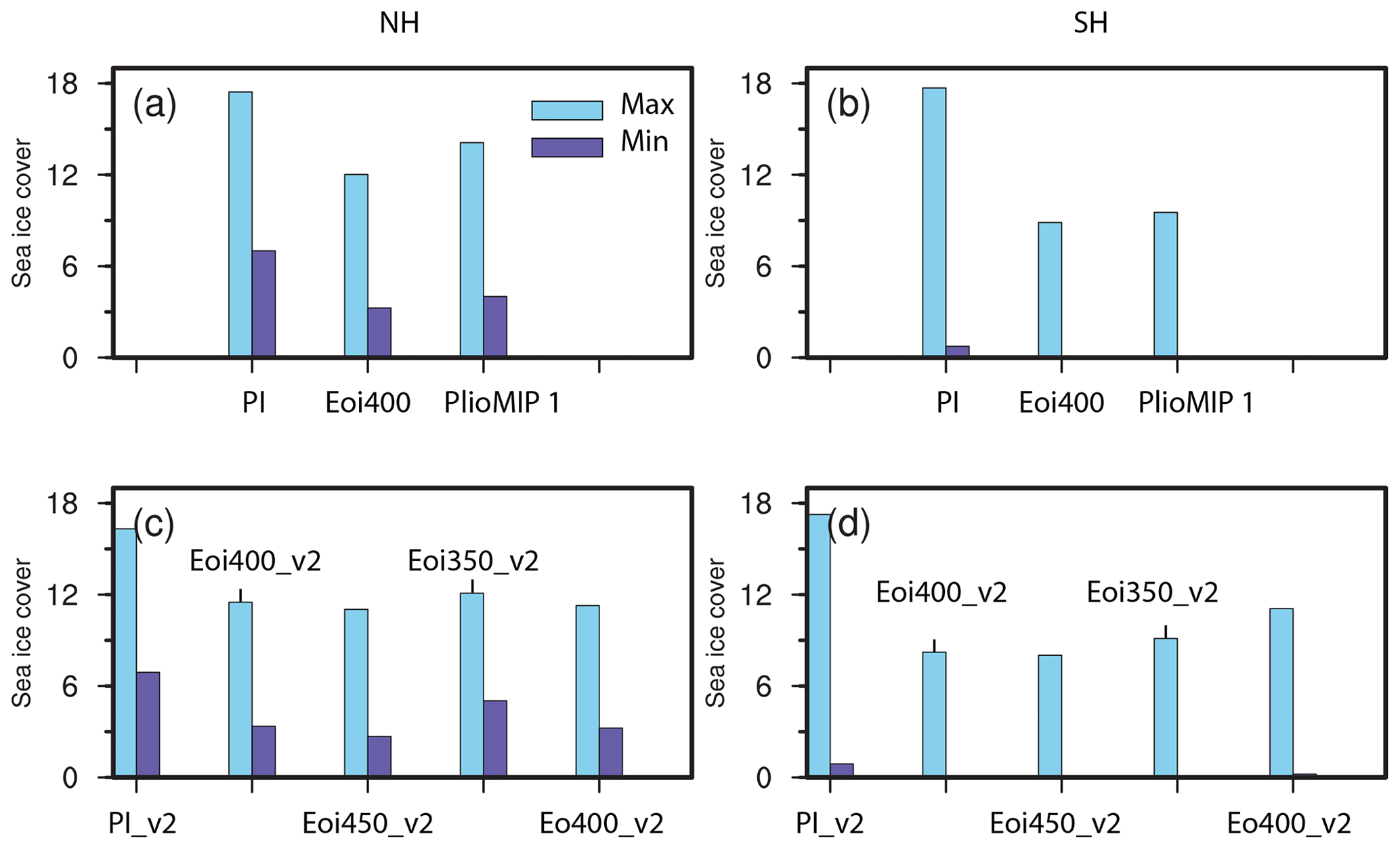
Figure 7Maximum and minimum sea ice cover for both hemispheres in each experiment (unit: 1×10⁶ km2).
The global mean annual precipitation rate increases by 0.14 mm d−1 in Eoi400 due to the vapor-varying capacity of the warmer atmosphere, and the increase is mostly confined to the global monsoon regions and tropical oceans. The increase in global mean precipitation rate as well as the monsoon area index (Fig. S2, calculated based on the method of Wang et al., 2008) in Eoi400 compared to PI is similar to that in PlioMIP1. However, regional discrepancies still exist between these two experiments: the precipitation rates in Eoi400 in the tropics and NH high latitudes are higher than those in PlioMIP1 by 0.03–0.05 mm d−1 because of the increased warming in Eoi400 in these regions. Regional differences also exist over mountainous regions (e.g., the Andes, the Rockies, the Tibetan Plateau, the Himalayas, and the Ethiopian Highlands) since the elevation over these regions is modified largely in PlioMIP2 compared to PlioMIP1 (Fig. 1). In East Africa, Eoi400 simulates an intensified precipitation than PlioMIP1, which is better consistent with proxy data from East Africa inferring a wet vegetation condition and hydrological systems during this period (Drapeau et al., 2014; Bonnefille, 2010). Apart from the high-latitude seaway change, the regional difference in topography between PlioMIP2 and PlioMIP1 can also contribute to the rainfall change. Further sensitivity studies are needed to verify it.
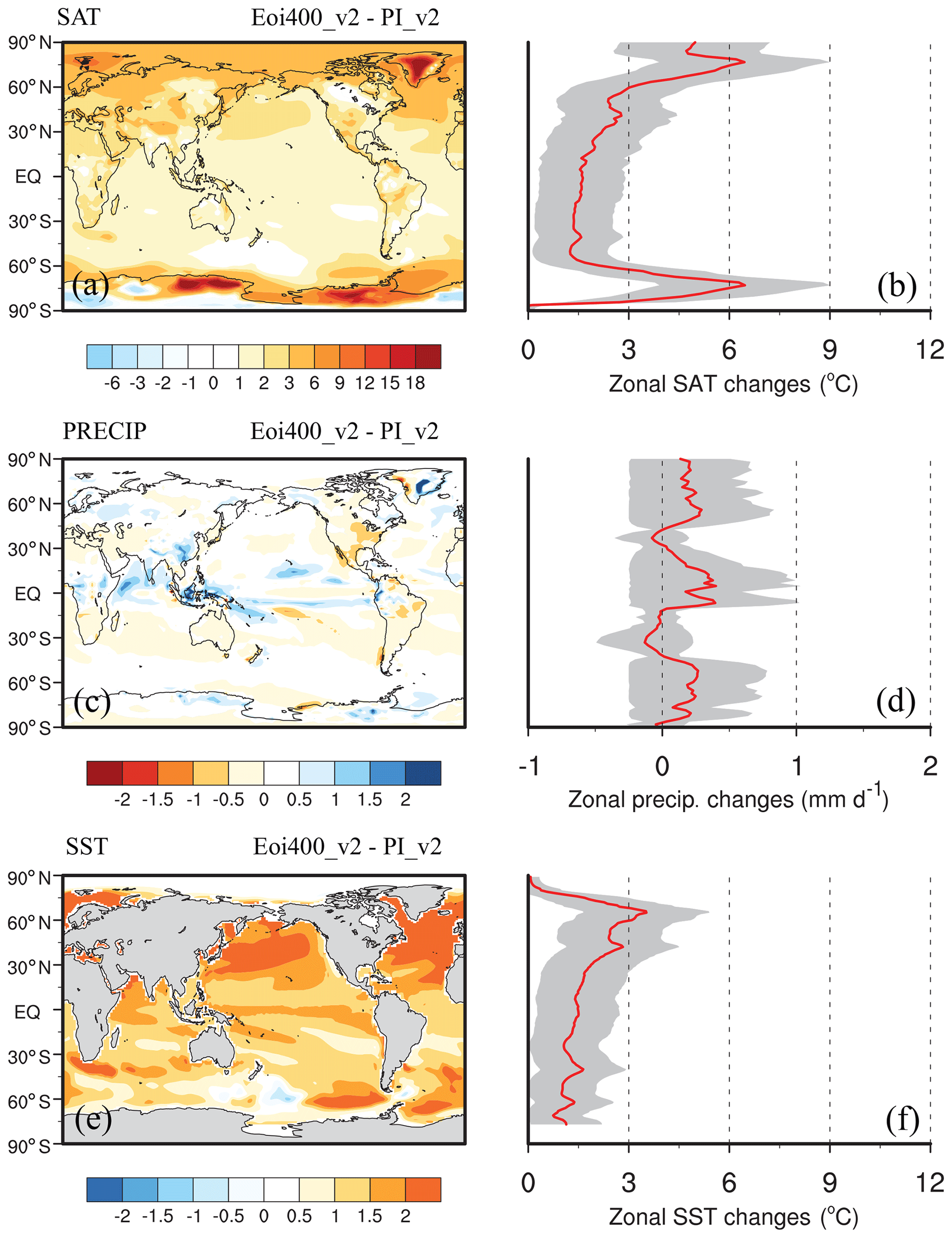
Figure 8Anomalies of mean annual SAT (a), mean annual precipitation (c) and mean annual SST (e) of Eoi400_v2 in comparison with the associated PI control experiment. Panels (b), (d), and (f) represent the zonal mean of related anomalies; the shaded area shows 1σ standard deviation.
4.1.2 Results in the ocean
The global mean annual SST of Eoi400 is 1.7 ∘C warmer compared to the pre-industrial one. It is 0.3 ∘C warmer than PlioMIP1, and the warming is largely confined to the mid- to high-latitude oceans of the Northern Hemisphere. The warming in Eoi400 relative to PlioMIP1 can be attributed to the closure of the Bering Strait and the Canadian Arctic Archipelago, which is the major difference in the boundary conditions between these two experiments. In the pre-industrial control run (Fig. 3a), the water flow through the Bering Strait is about 1.0 Sv (sverdrup), through which much fresher and warmer water from the North Pacific is transported to the Arctic Ocean. In Eoi400, as shown in Fig. 3b, the water currents from the North Pacific to the Arctic through the Bering Strait and from the Arctic to the Baffin Bay are shut down. Consequently, the Arctic seawater gets much denser and thus the wind-driven Beaufort Gyre and transpolar drift get weakened (Fig. 3c). The associated East Greenland Current and the Labrador Current get weaker, resulting in saltier conditions in these adjacent regions (Fig. 4b). Thus, the deep convection and the formation of North Atlantic Deep Water (Figs. 4c, 5b) over these regions enhance. The sea surface condition changes (compared to the PI) in the North Atlantic region in Eoi400 (Fig. 4) are in agreement with the CCSM4 model results of Otto-Bliesner et al. (2017). Accordingly, we observe a strengthened Gulf Stream and North Atlantic currents as well as an enhanced subpolar gyre (Fig. 3c), which can transport more heat to high latitudes (Fig. 6b) and may be linked to a stronger convection. Thus, a shoaled and enhanced AMOC (Atlantic Meridional Overturning Circulation) (+4.9 Sv) is observed in Eoi400, whereas the AMOC in PlioMIP1 was not much different from the modeled pre-industrial level (Fig. 5). The increased AMOC resulting from the closure of the Bering Strait and Canadian Arctic Archipelago is broadly consistent with previous studies by Hu et al. (2015), Kamae et al. (2016), and Chandan and Peltier (2017). However, the change in the AMOC strength in our PlioMIP2 simulation is much larger than in other models. Hu et al. (2015), using CCSM3 and CCSM2, with different climate backgrounds show that the AMOC responses to the closure of the Bering Strait are about 2–3 Sv. Chandan and Peltier (2016) show an increased AMOC strength by ∼2 Sv after closing the Bering Strait in the CCSM4 model. In the study of Kamae et al. (2016), with a different flux adjustment, they present a much stronger AMOC in their PlioMIP2 than their pre-industrial level. In fact, the simulated AMOC largely depends upon the vertical mixing schemes (Zhang et al., 2013). Although we observe an increase in the strength of AMOC (15.7 Sv) in our PlioMIP2 simulation conducted with IPSL-CM5A, the AMOC is still weaker than the modern observations (17.2 Sv, McCarthy et al., 2015). This is because the simulated modern AMOC (11 Sv) with this model is much weaker than the observations. Moreover, the simulated AMOC in PlioMIP1 with our model is also weaker than other models (Zhang et al., 2013). As shown in Fig. 6, the total heat transport in the PI control, Eoi400, and PlioMIP1 simulations is similar. The stronger AMOC in Eoi400 does indeed strengthen the northward heat transport in the Atlantic Ocean, while the weakened Pacific meridional ocean circulation in Eoi400 (PMOC, Fig. S3), which contrasts with the data-based findings by Burls et al. (2017), decreases the northward heat transport, thus leading to very slight change in total ocean heat transport. This compensation was also found by Chandan and Peltier (2017).
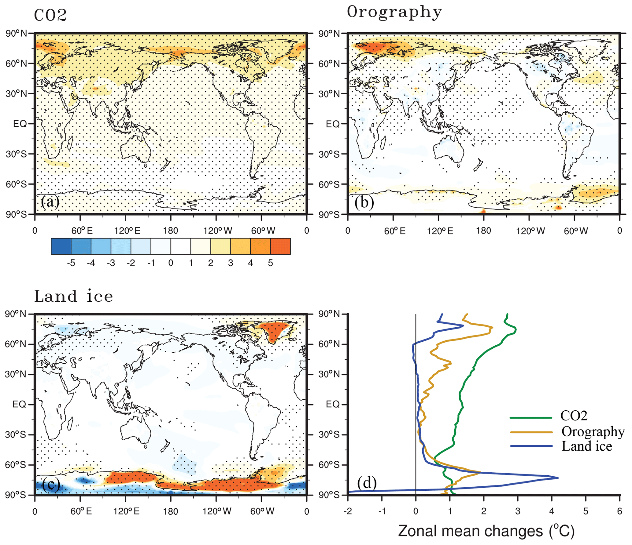
Figure 9The relative contribution of various boundary conditions (a CO2, b orography, c land ice) to the warmth of PlioMIP 2 and their zonal mean values (d). Stippling indicates regions where results are statistically significant at 99 % confidence criteria.
The simulated warm conditions at high latitudes prevent sea ice from expanding during the winter season and increase sea ice melt during the summer season (Fig. 7). When compared to the PI condition, sea ice extent in the Eoi400 decreases by 5.4 and 3.8 Mkm2 respectively for the winter and summer season in the NH. In the Southern Hemisphere (SH), sea ice extent reduces by 8.8 Mkm2 for the winter season and is nearly extinct during the summer. In comparison with PlioMIP1, NH sea ice cover in Eoi400 reduces by 2.1 and 0.8 Mkm2, respectively, for cold and warm season, but there is no large difference in SH between these two experiments. The largely decreased sea ice extent can amplify the warming in the high latitudes through its role as an insulation between the ocean and the atmosphere as well as positive albedo temperature feedback (Howell et al., 2014; Zheng et al., 2019). Reconstructed data in the Arctic Basin suggest the presence of seasonal rather than perennial sea ice in the Pliocene Arctic (Polyak et a., 2010; Moran et al., 2006), indicating a less or diminished summer sea ice cover. However, our IPSL model as well as half of participating models in PlioMIP1 cannot predict sea-ice-free conditions during the summer season (Howell et al., 2016). Reasons for this are discussed in Howell et al. (2016), who demonstrate the unreasonable sea ice albedo parameterization for the warmer condition.
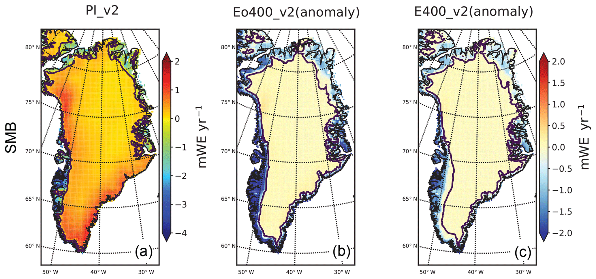
Figure 10Mean annual surface mass balance (SMB) in Greenland in the PI control experiment (a) and the anomalies of the SMB in Eo400_v2 (b) and E400_v2 (c) experiments in comparison with the PI control (unit: mWE (water equivalent) yr−1). The contour line indicates the zero value.
4.2 Pliocene runs with IPSL-CM5A2
4.2.1 Results from the core experiment Eoi400_v2
Figure 8 shows the anomalies of global mean annual near SAT (2 m temperature), precipitation rate, and SST between Eoi400_v2 and the pre-industrial control with the CM5A2model. The global mean SAT in Eoi400_v2 is 15.3 ∘C, which is 2.2 ∘C warmer than pre-industrial conditions with greater warming at high latitudes. It should be noted that the absolute SAT in Eoi400_v2 is greater than that obtained in Eoi400, while the SAT anomaly in Eoi400_v2 is lower than that in Eoi400. This is due to the cold bias correction in the new version of the IPSL model. IPSL-CM5A2 simulates a pre-industrial temperature that is warmer (Sepulchre et al., 2020) than the IPSL-CM5A pre-industrial one by 1.1 ∘C. The global mean annual precipitation rate increases by 0.13 mm d−1 in Eoi400_v2 compared to PI, which is comparable to the results obtained with IPSL-CM5A. In Eoi400_v2, the changes in the ocean conditions relative to the pre-industrial control are similar to changes seen with Eoi400. The global mean annual SST in Eoi400_v2 is 0.7 ∘C warmer than Eoi400, the AMOC strength (Fig. S4) in Eoi400_v2 is 17.9 Sv, which is 2.2 Sv larger than Eoi400, while the AMOC anomaly is about 4.7 Sv relative to its pre-industrial level of 13.2 Sv. The magnitude of this anomaly is close to the result obtained with IPSL-CM5A, indicating a coherent response of the AMOC to the same changes in boundary conditions. The sea ice cover is also largely decreased due to the warming at high latitudes (Fig. 7).
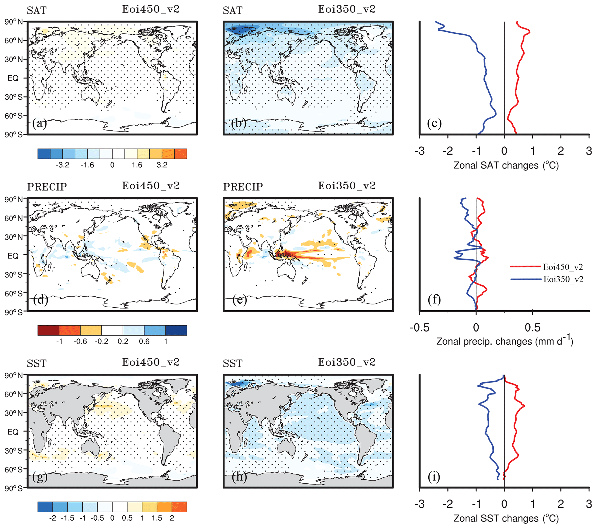
Figure 11Anomalies of mean annual SAT, mean annual precipitation rate, and mean annual SST for Eoi450_v2 (a, d, g) and Eoi350_v2 (b, e, h) in comparison with Eoi400_v2. The last column (c, f, i) of this panel shows the zonal mean of related anomalies (red and blue lines, respectively, represent the results of Eoi450_v2 and Eoi350_v2). Stippling indicates regions where results are statistically significant at 99 % confidence criteria.
4.2.2 Relative importance of various boundary conditions in MIS KM5c warmth
Figure 9 shows the relative contribution of various boundary conditions (CO2 – a; orography – b; and land ice – c) to the warming during MIS KM5c as obtained using the linear decomposition method. Among these forcings, the increase in pCO2 by 120 ppmv (from 280 to 400 ppmv) plays the most important role in both the annual (+1.4 ∘C) and seasonal SAT (+1.38 ∘C and +1.48 ∘C, respectively, during the summer and winter). The changes to orography in PlioMIP2 also exert an important influence on the annual mean warming (+0.51 ∘C), especially in the North Atlantic and Barents Sea regions. However, changes to the orography decrease the temperature in the NH mid- to high-latitude inland regions, which may result from changes in North Pacific circulation. Seasonally, the orography changes contribute more to the warming in summer (+0.65 ∘C) than to that in winter (+0.38 ∘C). The impact of smaller ice sheets is largely restricted to the high-latitude regions and is less important than the other two forcing factors in the North Pole region but plays a key role in the warming of the South Pole region. The mean annual warming resulting from the smaller ice sheets is about 0.25 ∘C which is close to the contribution in both summer and winter seasons, indicating that the ice sheet contribution is seasonally invariant. The residual impact besides the pCO2, orography and land ice forcings is relatively small and negligible when making the linear decomposition of the forcing factors. These results are in agreement with those of Chandan and Peltier (2018), who applied the nonlinear decomposition of Lunt et al. (2012) to diagnose the contributions of the forcing factors
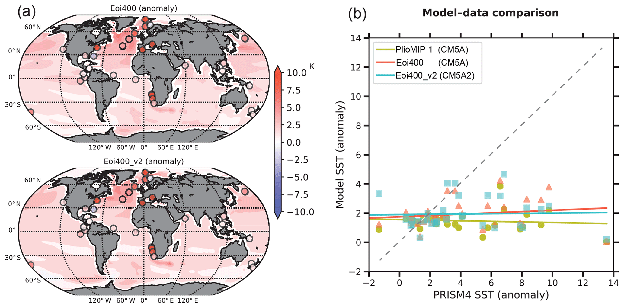
Figure 12SST model–data comparison. (a) Modeled mean annual SST anomalies of MIS KM5c (relative to PI controls; shaded area) and reconstructed MIS KM5c SST anomalies (relative to near-pre-industrial data; circle markers). (b) The relationship between modeled SST anomalies and PRISM4 data anomalies.
4.2.3 Greenland Ice Sheet instability under MIS KM5c warmth
To understand the extent to which the Greenland Ice Sheet (GrIS) could be sustained under the warmth of MPWP, we impose the modern GrIS into the Pliocene simulation (Eo400_v2). We obtain the GrIS surface mass balance (SMB) by applying the outputs (monthly near-surface air temperature and precipitation) of each climate experiment (PI_v2, Eo400_v2, E400_v2) to the GRenoble Ice-Shelf and Land-Ice model (GRISLI) (Ritz et al., 2001), in which the algorithm for the SMB is calculated. In comparison with the PI control (Fig. 10a), the mean annual SMB in Greenland in Eo400_v2 (Fig. 10b) is strongly negative around the coastal regions, indicating vulnerable conditions along the coastal ice sheet and ice shelves. This negative SMB condition largely results from the increased summer temperature, which leads to enhanced ablation in these regions (Fig. S5). The mean annual SMB condition in Eo400_v2 is similar to that in modern conditions (E400_v2; Fig. 10c). However, the warmer conditions in Eo400_v2 bring more precipitation in south and northwest Greenland, leading to enhanced accumulation (Fig. S5); thus we observe increased SMB in these areas as compared to the PI control condition. In E400_v2, we also have increased SMB in these regions, but it is much weaker than that in Eo400_v2, due to the different paleogeography settings as discussed earlier. Although these snapshot results cannot quantify the impact of the warm climate on the modern GrIS extent, which needs another series of climate-model–ice-sheet-model experiments, the results we get here can also herald the vulnerability of the GrIS under such warm climate conditions.
4.2.4 pCO2 uncertainties in MIS KM5c warmth
Figure 11 depicts the anomalies of global mean annual SAT, precipitation rate, and SST in Eoi450_v2 and Eoi350_v2 compared to the core experiment Eoi400_v2. By increasing pCO2 by 50 ppmv in Eoi450_v2, global climate gets slightly warmer (+0.48 ∘C) and the warming at high latitudes is larger (+0.7 ∘C). However, when lowering pCO2 by 50 ppmv in Eoi350_v2, the change in climate is more important than that in Eoi450_v2, since we observe a global cooling of 0.71 ∘C and a cooling of 1.29 ∘C over NH high latitudes. This asymmetric pattern in temperature response to changes in pCO2 largely results from changes to surface albedo associated with snow cover (not shown here). In Eoi450_v2, the mean annual snowfall decreases by 6 % between 40 and 80∘ N when comparing it to Eoi400_v2, while Eoi350_v2 shows an increase by 30 % (not shown). The asymmetric pattern between Eoi450_v2 and Eoi350_v2 is also found in the changes in precipitation rates: global climate gets slightly moister with a global precipitation rate that has increased by 0.02 mm d−1 (+15 %) in Eoi450_v2, while in Eoi350_v2, the global precipitation rate reduces by 0.04 mm d−1 (−31 %), and this reduction is more important in the tropical regions. Thus, our results can also show that the response of the IPSL coupled model to changing pCO2 from 350 to 400 ppm is larger than from 400 to 450 ppm.
However, in the ocean, the increase or decrease in SSTs resulting from increasing or lowering pCO2 by 50 ppmv is nearly the same magnitude. The AMOC strengths are also similar between Eoi450_v2 (17.4 Sv) and Eoi350_v2 (17.6 Sv) (Fig. S4). Nevertheless, the changes in sea ice cover in these two experiments are unlike each other (Fig. 7). As in Eoi450_v2, the sea ice covers decrease slightly relative to Eoi400_v2 for both hemispheres (decreased by 0.2–0.5 Mkm2 during the cold season and decreased by 0.01–0.2 Mkm2 during the warm season), whereas in Eoi350_v2, the sea ice cover expands for both hemispheres, especially during the warm season in the NH (+1.7 Mkm2).
4.3 Model–data comparison
Figure 12 shows the simulated mean annual SST anomalies (relative to PI experiments) of both core experiments (Eoi400, Eoi400_v2), together with the reconstructed SST (3.20–3.21 Ma; Foley and Dowsett, 2019) anomalies relative to near-pre-industrial data (1870–1900; Rayner et al., 2003). The simulated SST anomalies in both core experiments are generally in phase with the reconstructed data. Some extremely warm sites are in disagreement with model results (e.g., drilling sites in the North Greenland Sea, in the Mediterranean, and in the Benguela Current region). Overall, the simulated MIS KM5c SSTs generally underestimate the warming that is inferred from proxies, especially for the sites showing warming higher than 4 ∘C (Fig. 12b). Of the three experiments (PlioMIP1, Eoi400, Eoi400_v2), both Eoi400 and Eoi400_v2 show increased warming in the mid- to high latitudes as compared to the PlioMIP1 result. However, despite the increased warming exhibited by our PlioMIP2 simulation, there is still an obvious disagreement between model and proxy, for which model performance is partly to blame. However, the interpretation of the reconstructed data can also affect the data–model comparison. Conventionally, SSTs are reconstructed from paleothermometry assuming they represent annual mean values, whereas it has been shown that they can represent seasonal temperatures, for example representing the warmest summer month in the North Atlantic (NATL) (Leduc et al., 2017) and in the Benguela Current (Leduc et al., 2014). If we compare the reconstructed SST anomalies with modeled SST anomalies for the warmest summer month rather than the mean annual anomalies for the NATL and the Benguela region (Fig. S6), the discrepancies between model and data are reduced. To understand the disagreement well, more studies are needed with regard to data interpretation as well as the multi-model comparison.
In this paper, we describe the results of modeling the warm interglacial MIS KM5c (3.205 Ma), located in the MPWP interval of 3.0–3.3 Ma, while driving the model with the new PRISM4 boundary conditions (Dowsett et al., 2016). Two versions of the core Pliocene experiments, namely Eoi400 and Eoi400_v2, are conducted on two versions of the IPSL coupled model: IPSL-CM5A and IPSL-CM5A2. Four tiered experiments (E400_v2, Eoi450_v2, Eoi350_v2, Eo400_v2) are also conducted with IPSL-CM5A2 to study the relative contribution of various forcing factors towards the warming of climate. The new PRISM4 boundary conditions produce an enhanced global warming in MIS KM5c, especially over the mid- to high-latitude oceans compared to the results from PlioMIP phase 1. The enhanced warming can be largely attributed to changes to high-latitude seaways which strengthen AMOC and transport more heat to high latitudes and to the reduction in the spatial extent of ice sheets and sea ice which decreases the outgoing shortwave radiation. The warming in MIS KM5c simulated with either of our models is weaker than those found in other studies (e.g. Kamae et al., 2016; Chandan and Peltier, 2017). In both our two core experiments, AMOC strength increases remarkably (+4.7 Sv) in comparison to PI controls due to the closure of the Bering Strait and the north Canadian Arctic Archipelago regions. This result agrees with other studies (Kamae et al., 2016; Hu et al., 2015), but the extent of the increase of the AMOC depends highly upon the processes included in the ocean models.
In addition to the orography changes, changes to the concentration of greenhouse gases and changes to the configuration of high-latitude ice play important roles in the polar amplification; e.g., the reduced ice sheets over Antarctica play a key role in the warming of the high latitudes of the Southern Hemisphere. Surface mass balance analysis shows that the modern GrIS is vulnerable around the coastal regions under the warm conditions of the MPWP as well as present conditions. The model response to changes to pCO2 ( ppmv) was found to not be symmetric with respect to the surface air temperature, which is likely due to the nonlinear response of snow cover and sea ice extent. When snow cover and sea ice extent are reduced in area and duration, the sensitivity of climate model to the growing pCO2 may have a weaker thermal impact, in contrast to the near-linear response of global surface air temperature to the cumulative emissions of pCO2 in both the present short-term observations and transient modeling scenarios for the future. Finally, further model intercomparison work and data–model comparison work are needed to better understand the role of variable boundary conditions and the internal climatic processes in modeling the Pliocene warming climate.
Climatological averages of each simulation in NetCDF format will be uploaded to the PlioMIP2 data repository soon. It is accessible in the meantime by contacting the authors. Specific data requests should be sent to the lead author (ning.tan@mails.iggcas.ac.cn). All PlioMIP2 boundary conditions are available on the USGS PlioMIP2 web page https://www.usgs.gov/centers/fbgc/science/pliocene-research-interpretation-and-synoptic-mapping-prism4?qt-science_center_objects=0#qt-science_center_objects (last access: 28 November 2019).
The supplement related to this article is available online at: https://doi.org/10.5194/cp-16-1-2020-supplement.
NT, GR, and CC designed the study. NT conducted the model setup, spin-up, and major data analysis and wrote the paper. YS, CC, CD, and ZG contributed to discussing the data analysis and the structure of this work. PS provided the IPSL-CM5A2 information and its related control run simulation. All co-authors helped to improve this paper. Correspondence and requests for materials should be addressed to NT.
The authors declare that they have no conflict of interest.
This article is part of the special issue “PlioMIP Phase 2: experimental design, implementation and scientific results”. It is not associated with a conference.
We thank Oliver Marti and Jean Baptiste Ladant for their help on the model setup. Many thanks to editor Aisling Dolan and two anonymous reviewers for their useful comments, which improved the quality of the manuscript. This study was performed using HPC resources from GENCI-TGCC under the allocation 2019-A0050102212.
This research has been supported by the French State Program Investissements d'Avenir (managed by ANR), the ANR HADOC project (grant no. ANR-17-CE31-0010), the Basic Science Center Project of the National Science Foundation of China (grant no. 41888101), and the Strategic Priority Research Program (grant no. XDB 26000000).
This paper was edited by Aisling Dolan and reviewed by two anonymous referees.
Bartoli, G., Hönisch, B., and Zeebe, R. E.: Atmospheric CO2 decline during the Pliocene intensification of Northern Hemisphere glaciations, Paleoceanography, 26, PA4213, https://doi.org/10.1029/2010PA002055, 2011.
Blanke, B. and Delecluse, P.: Variability of the Tropical Atlantic Ocean Simulated by a General Circulation Model with Two Different Mixed-Layer Physics, J. Phys. Oceanogr., 23, 1363–1388,1993.
Bonnefille, R.: Cenozoic vegetation, climate changes and hominid evolution in tropical Africa, Global Planet. Change, 72, 390–411, 2010.
Brigham-Grette, J., Melles, M., Minyuk, P., Andreev, a., Tarasov, P., DeConto, R., Koenig, S., Nowaczyk, N., Wennrich, V., Rosen, P., Haltia, E., Cook, T., Gebhardt, C., Meyer-Jacob, C., Snyder, J., and Herzschuh, U.: Pliocene Warmth, Polar Amplification, and Stepped Pleistocene Cooling Recorded in NE Arctic Russia, Science, 340, 1421–1427, https://doi.org/10.1126/science.1233137, 2013.
Burls, N. J., Fedorov, A. V, Sigman, D. M., Jaccard, S. L., Tiedemann, R., and Haug, G. H.: Active Pacific meridional overturning circulation (PMOC) during the warm Pliocene, Sci. Adv., 3, e1700156, https://doi.org/10.1126/sciadv.1700156, 2017.
Burls, N. J. and Fedorov, A. V.: Simulating Pliocene warmth and a permanent El Niño-like state: The role of cloud albedo, Paleoceanography, 29, 893–910, https://doi.org/10.1002/2014PA002644, 2014.
Chandan, D. and Peltier, W. R.: Regional and global climate for the mid-Pliocene using the University of Toronto version of CCSM4 and PlioMIP2 boundary conditions, Clim. Past, 13, 919–942, https://doi.org/10.5194/cp-13-919-2017, 2017.
Chandan, D. and Peltier, W. R.: On the mechanisms of warming the mid-Pliocene and the inference of a hierarchy of climate sensitivities with relevance to the understanding of climate futures, Clim. Past, 14, 825–856, https://doi.org/10.5194/cp-14-825-2018, 2018.
Contoux, C., Ramstein, G., and Jost, A.: Modelling the mid-Pliocene Warm Period climate with the IPSL coupled model and its atmospheric component LMDZ5A, Geosci. Model Dev., 5, 903–917, https://doi.org/10.5194/gmd-5-903-2012, 2012.
Contoux, C., Dumas, C., Ramstein, G., Jost, A., and Dolan, A. M.: Modelling Greenland ice sheet inception and sustainability during the Late Pliocene, Earth Planet. Sci. Lett., 424, 295–305, https://doi.org/10.1016/j.epsl.2015.05.018, 2015.
Cravatte, S., Madec, G., Izumo, T., Menkès, C., and Bozec, A.: Progress in the 3-D circulation of the eastern equatorial Pacific in a cli-mate ocean model, Ocean Modell., 17, 28–48, https://doi.org/10.1016/j.ocemod.2006.11.003, 2007.
Crowley, T. J.: Modeling pliocene warmth, Quat. Sci. Rev., 10, 275–282, 1991.
Dolan, A. M., Hunter, S. J., Hill, D. J., Haywood, A. M., Koenig, S. J., Otto-Bliesner, B. L., Abe-Ouchi, A., Bragg, F., Chan, W.-L., Chandler, M. A., Contoux, C., Jost, A., Kamae, Y., Lohmann, G., Lunt, D. J., Ramstein, G., Rosenbloom, N. A., Sohl, L., Stepanek, C., Ueda, H., Yan, Q., and Zhang, Z.: Using results from the PlioMIP ensemble to investigate the Greenland Ice Sheet during the mid-Pliocene Warm Period, Clim. Past, 11, 403–424, https://doi.org/10.5194/cp-11-403-2015, 2015.
Dowsett, H., Dolan, A., Rowley, D., Moucha, R., Forte, A. M., Mitrovica, J. X., Pound, M., Salzmann, U., Robinson, M., Chandler, M., Foley, K., and Haywood, A.: The PRISM4 (mid-Piacenzian) paleoenvironmental reconstruction, Clim. Past, 12, 1519–1538, https://doi.org/10.5194/cp-12-1519-2016, 2016.
Dowsett, H. J., Chandler, M. A., and Robinson, M. M.: Surface temperatures of the mid-pliocene north atlantic ocean: implications for future climate, Philos. T. Roy. Soc. A, 367, 69–84, 2009.
Dowsett, H. J., Robinson, M. M., Haywood, A. M., Hill, D. J., Dolan, A. M., Stoll, D. K., Chan, W.-L., Abe-Ouchi, A., Chandler, M. A.,Rosenbloom, N. A., Otto-Bliesner, B. L., Bragg, F. J., Lunt, D. J., Foley, K. M., and Riesselman, C. R.: Assessing confidence in Pliocene sea surface temperatures to evaluate predictive models, Nat. Clim. Change, 2, 365–371, https://doi.org/10.1038/nclimate1455, 2012.
Drapeau, M. S. M., Bobe, R., Wynn, J. G., Campisano, C. J., Dumouchel, L., and Geraads, D.: The Omo Mursi Formation: A window into the East African Pliocene, J. Hum. Evol., 75, 64–79, https://doi.org/10.1016/j.jhevol.2014.07.001, 2014.
Ducoudré, N. I., Laval, K., and Perrier, A.: SECHIBA, a new set of parameterizations of the hydrologic exchanges at the land- atmosphere interface within the LMD atmospheric general circulation model, J. Climate, 6, 248–273, 1993.
Dufresne, J.-L., Foujols, M.-A., Denvil, S., Caubel, A., Marti, O., Aumont, O., Balkanski, Y., Bekki, S., Bellenger, H., Benshila, R., Bony, S., Bopp, L., Braconnot, P., Brockmann, P., Cadule, P., Cheruy, F., Codron, F., Cozic, A., Cugnet, D., Noblet, N., Duvel, J.-P., Ethé, C., Fairhead, L., Fichefet, T., Flavoni, S., Friedlingstein, P., Grandpeix, J.-Y., Guez, L., Guilyardi, E., Hauglustaine, D., Hourdin, F., Idelkadi, A., Ghattas, J., Joussaume, S., Kageyama, M., Krinner, G., Labetoulle, S., Lahellec, a., Lefebvre, M.-P., Lefevre, F., Levy, C., Li, Z. X., Lloyd, J., Lott, F., Madec, G., Mancip, M., Marchand, M., Masson, S., Meurdesoif, Y., Mignot, J., Musat, I., Parouty, S., Polcher, J., Rio, C., Schulz, M., Swingedouw, D., Szopa, S., Talandier, C., Terray, P., Viovy, N., and Vuichard, N.: Climate change projections using the IPSL-CM5 Earth System Model: from CMIP3 to CMIP5, Vol. 40, https://doi.org/10.1007/s00382-012-1636-1, 2013.
Fedorov, A. V., Brierley, C. M., Lawrence, K. T., Liu, Z., Dekens, P. S., and Ravelo, A. C.: Patterns and mechanisms of early Pliocene warmth, Nature, 496, 43–49, https://doi.org/10.1038/nature12003, 2013.
Foley, K. M. and Dowsett, H. J.: Community sourced mid-Piacenzian sea surface temperature (SST) data: U.S. Geological Survey data release, https://doi.org/10.5066/P9YP3DTV, 2019.
Haywood, A. M., Dolan, A. M., Pickering, S. J., Dowsett, H. J., McClymont, E. L., Prescott, C. L., Salzmann, U., Hill, D. J., Hunter, S. J., Lunt, D. J., Pope, J. O., and Valdes, P. J.: On the identification of a Pliocene time slice for data-model comparison, Philos. T. Roy. Soc. A, 371, 20120515, https://doi.org/10.1098/rsta.2012.0515, 2013.
Haywood, A. M., Dowsett, H. J., Dolan, A. M., Rowley, D., Abe-Ouchi, A., Otto-Bliesner, B., Chandler, M. A., Hunter, S. J., Lunt, D. J., Pound, M., and Salzmann, U.: The Pliocene Model Intercomparison Project (PlioMIP) Phase 2: scientific objectives and experimental design, Clim. Past, 12, 663–675, https://doi.org/10.5194/cp-12-663-2016, 2016.
Haywood, A. M., Dowsett, H. J., and Dolan, A. M.: Integrating geological archives and climate models for the mid-Pliocene warm period, Nat. Commun., 7, 10646, https://doi.org/10.1038/ncomms10646, 2016.
Hill, D. J.: Modelling Earth's Cryosphere during Pliocene Warm Peak, PhD thesis, University of Bristol, United Kingdom, p. 368, 2009.
Hourdin, F., Musat, I., Bony, S., Braconnot, P., Codron, F., Dufresne, J.-L., Fairhead, L., Filiberti, M.-A., Friedlingstein, P., Grandpeix, J.-Y., Krinner, G., LeVan, P., Li, Z.-X., and Lott, F.: The LMDZ4 general circulation model: climate performance and sensitivity to parametrized physics with emphasis on tropical convection, Clim. Dynam., 27, 787–813, https://doi.org/10.1007/s00382-006-0158-0, 2006.
Hourdin, F., Foujols, M.-A., Codron, F., Guemas, V., Dufresne, J.-L., Bony, S., Denvil, S., Guez, L., Lott, F., Ghattas, J., Braconnot, P., Marti, O., Meurdesoif, Y., and Bopp, L.: Impact of the LMDZ atmospheric grid configuration on the climate and sensitivity of the IPSL-CM5A coupled model, Clim. Dynam., 40, 2167–2192, https://doi.org/10.1007/s00382-012-1411-3, 2013.
Howell, F. W., Haywood, A. M., Dolan, A. M., Dowsett, H. J., Francis, J. E., Hill, D. J., and Wade, B. S.: Can uncertainties in sea ice albedo reconcile patterns of data-model discord for the Pliocene and 20th/21st centuries?, Geophys. Res. Lett., 41, 2011–2018, https://doi.org/10.1002/2013GL058872, 2014.
Howell, F. W., Haywood, A. M., Otto-Bliesner, B. L., Bragg, F., Chan, W.-L., Chandler, M. A., Contoux, C., Kamae, Y., Abe-Ouchi, A., Rosenbloom, N. A., Stepanek, C., and Zhang, Z.: Arctic sea ice simulation in the PlioMIP ensemble, Clim. Past, 12, 749–767, https://doi.org/10.5194/cp-12-749-2016, 2016.
Hu, A., Meehl, G. A., Han, W., Otto-Bliestner, B., Abe-Ouchi, A., and Rosenbloom, N.: Effects of the Bering Strait closure on AMOC and global climate under different background climates, Prog. Oceanogr., 132, 174–196, https://doi.org/10.1016/j.pocean.2014.02.004, 2015.
Jost, A., Fauquette, S., Kageyama, M., Krinner, G., Ramstein, G., Suc, J.-P., and Violette, S.: High resolution climate and vegetation simulations of the Late Pliocene, a model-data comparison over western Europe and the Mediterranean region, Clim. Past, 5, 585–606, https://doi.org/10.5194/cp-5-585-2009, 2009.
Kageyama, M., Braconnot, P., Bopp, L., Caubel, A., Foujols, M.-A., Guilyardi, E., Khodri, M., Lloyd, J., Lombard, F., Mariotti, V., Marti, O., Roy, T., and Woillez, M.-N.: Mid-Holocene and Last Glacial maximum climate simulations with the IPSL model – Part I: comparing IPSL_CM5A to IPSL_CM4, Clim. Dynam., 40, 2447–2468, https://doi.org/10.1007/s00382-012-1488-8, 2013.
Kamae, Y., Yoshida, K., and Ueda, H.: Sensitivity of Pliocene climate simulations in MRI-CGCM2.3 to respective boundary conditions, Clim. Past, 12, 1619–1634, https://doi.org/10.5194/cp-12-1619-2016, 2016.
Kasahara, A.: Computational aspects of numerical models for weather prediction and climate simulation, in: Methods in computational physics, 1–66, 1977.
Koenig, S. J., Dolan, A. M., de Boer, B., Stone, E. J., Hill, D. J., DeConto, R. M., Abe-Ouchi, A., Lunt, D. J., Pollard, D., Quiquet, A., Saito, F., Savage, J., and van de Wal, R.: Ice sheet model dependency of the simulated Greenland Ice Sheet in the mid-Pliocene, Clim. Past, 11, 369–381, https://doi.org/10.5194/cp-11-369-2015, 2015.
Krinner, G., Viovy, N., de Noblet-Ducoudre, N., Ogee, J., Polcher, J.and Friedlingstein, F., Ciais, P., Sitch, S., and Prentice, I. C.: A dynamic global vegetation model for studies of the coupled atmosphere-biosphere system, Global Biogeochem. Cy., 19, GB1015, https://doi.org/10.1029/2003GB002199, 2005.
Leduc, G., Garbe-Schönberg, D., Regenberg, M., Contoux, C., Etourneau, J., and Schneider, R.: The late Pliocene Benguela upwelling status revisited by means of multiple temperature proxies, Geochem. Geophys., 15, 475–491, https://doi.org/10.1002/2013GC004940, 2014.
Leduc, G., Herbert, C. T., Blanz, T., Martinez, P., and Schneider, R.: Contrasting evolution of sea surface temperature in the Benguela upwelling system under natural and anthropogenic climate forcings, Geophys. Res. Lett., 37, L20705, https://doi.org/10.1029/2010GL044353, 2010.
Leduc, G., De Garidelthoron, T., Kaiser, J., Bolton,C., and Contoux, C.: Databases for sea surface paleotemperature based on geochemical proxies from marine sediments: implications for model-data comparisons, Quaternaire, 28, 141–148, 2017.
Lévy, M., Estublier, A., and Madec, G.: Choice of an advection scheme for biogeochemical models, Geophys. Res. Lett., 28, 3725–3728, https://doi.org/10.1029/2001GL012947, 2001.
Madec, G. and the NEMO team: NEMO ocean engine, Note du Pole de modelisation, Institut Pierre-Simon Laplace (IPSL), France, No 27, ISSN NO 1288–1619, 2008.
Madec, G. and Imbard, M.: A global ocean mesh to overcome the North Pole singularity, Clim. Dynam., 12, 381–388, https://doi.org/10.1007/BF00211684, 1996.
Martínez-Botí, M. a., Foster, G. L., Chalk, T. B., Rohling, E. J., Sexton, P. F., Lunt, D. J., Pancost, R. D., Badger, M. P. S., and Schmidt, D. N.: Plio-Pleistocene climate sensitivity evaluated using high-resolution CO2 records, Nature, 518, 49–54, https://doi.org/10.1038/nature14145, 2015.
McCarthy, G., Smeed, D., Johns, W., Frajka-Williams, E., Moat, B., Rayner, D., Baringer, M., Meinen, C., Collins, J., and Bryden,H.: Measuring the Atlantic meridional overturning circulation at 26∘ N, Prog. Oceanogr., 130, 91–111, 2015.
Miller, K. G., Wright, J. D., Browning, J. V., Kulpecz, A., Kominz, M., Naish, T. R., Cramer, B. S., Rosenthal, Y., Peltier, W. R., and Sosdian, S.: High tide of the warm Pliocene: Implications of global sea level for Antarctic deglaciation, Geology, 40, 407, https://doi.org/10.1130/G32869.1, 2012.
Moran, K., Backman, J., and Farrell, J. W.: Deepwater drilling in the Arctic Ocean's permanent sea ice, https://doi.org/10.2204/iodp.proc.302.1062005, 2006.
O'Brien, C. L., Foster, G. L., Martínez-Botí, M. A., Abell, R., Rae, J. W., and Pancost, R. D.: High sea surface temperatures in tropicalwarm pools during the Pliocene, Nat. Geosci., 7, 606–611, 2014.
Otto-Bliesner, B. L., Jahn, A., Feng, R., Brady, E. C., Hu, A., and Löfverström, M.: Amplified North Atlantic warming in the late Pliocene by changes in Arctic gateways, Geophys. Res. Lett., 44, 957–964, https://doi.org/10.1002/2016GL071805, 2017.
Pagani, M., Liu, Z., LaRiviere, J., and Ravelo, A. C.: High Earth-system climate sensitivity determined from Pliocene carbon dioxide concentrations, Nat. Geosci., 3, 27–30, https://doi.org/10.1038/ngeo724, 2010.
Polyak, L., Alley, R. B., Andrews, J. T., Brigham-Grette, J., Cronin, T. M., Darby, D. A., and Jennings, A. E.: History of sea ice in the Arctic, Quat. Sci. Rev., 29, 1757–1778, 2010.
Pound, M. J., Tindall, J., Pickering, S. J., Haywood, A. M., Dowsett, H. J., and Salzmann, U.: Late Pliocene lakes and soils: a global data set for the analysis of climate feedbacks in a warmer world, Clim. Past, 10, 167–180, https://doi.org/10.5194/cp-10-167-2014, 2014.
Ravelo, A., Dekens, P., and McCarthy, M.: Evidence for El Niño-like conditions during the Pliocene, GSA Today, 16, 4–11, 2006.
Rayner, N. A. A., Parker, D. E., Horton, E. B., Folland, C. K., Alexander, L. V., Rowell, D. P., and Kaplan, A.: Global analyses of sea surface temperature, sea ice, and night marine air temperature since the late nineteenth century, J. Geophys. Res., 108, D14, https://doi.org/10.1029/2002JD002670, 2003.
Ritz, C., Rommelaere, V., and Dumas, C.: Modeling the evolution of Antarctic ice sheet over the last 420 000 years: Implications for altitude changes in the Vostok region, J. Geophys. Res., 106, D23, https://doi.org/10.1029/2001JD900232, 2001.
Rybczynski, N., Gosse, J. C., Harington, C. R., Wogelius, R. A., Hidy, A. J., and Buckley, M.: Mid-Pliocene warm-period deposits in the High Arctic yield insight into camel evolution, Nat. Commun., 4, 1550, doi:10.1038/ncomms2516, 2013.
Sadourny, R. and Laval, K.: January and July performance of the LMD general circulation model, in: New perspectives in climate modeling, edited by: Berger, A. and Nicolis, C., Elsevier, Amsterdam, 173–197, 1984.
Salzmann, U., Haywood, A. M., Lunt, D. J., Valdes, P. J., and Hill, D. J.: A new global biome reconstruction and data-model comparison for the Middle Pliocene, Global Ecol. Biogeogr., 17, 432–447, https://doi.org/10.1111/j.1466-8238.2008.00381.x, 2008.
Seki, O., Foster, G. L., Schmidt, D. N., Mackensen, A., Kawamura, K., and Pancost, R. D.: Alkenone and boron-based Pliocene pCO2 records, Earth Planet. Sci. Lett., 292, 201–211, https://doi.org/10.1016/j.epsl.2010.01.037, 2010.
Sitch, S., Smith, B., Prentice, C., Arneth, A., Bondeau, A., Cramer, W., Kaplan, J. O., Levis, S., Lucht, W., Sykes, M. T., and Thonicke, K.: Evaluation of ecosystem dynamics, plant geography and terrestrial carbon cycling in the LPJ dynamic vegetation model, Glob. Change Biol., 9, 161–185, 2003.
Tierney, J. E., Haywood, A. M., Feng, R., Bhattacharya, T., and Otto-Bliesner, B. L.: Pliocene warmth consistent with greenhouse gas forcing, Geophys. Res. Lett., 46, 9136–9144, https://doi.org/10.1029/2019GL083802, 2019.
Valcke, S.: OASIS3 user guide (prism 2-5), PRISM-Support Initiative Report No 3, p. 64, 2006.
Wara, M. W., Ravelo, A. C., and Delaney, M. L.: Permanent El Niño-Like Conditions During the Pliocene Warm Period, Science, 309, 758–761, https://doi.org/10.1126/science.1114760, 2005.
Zhang, Y. G., Pagani, M., and Liu, Z.: A 12-Million-Year Temperature History of the Tropical Pacific Ocean, Science, 344, 84–87, https://doi.org/10.1126/science.1246172, 2014.
Zhang, Z.-S., Nisancioglu, K. H., Chandler, M. A., Haywood, A. M., Otto-Bliesner, B. L., Ramstein, G., Stepanek, C., Abe-Ouchi, A., Chan, W.-L., Bragg, F. J., Contoux, C., Dolan, A. M., Hill, D. J., Jost, A., Kamae, Y., Lohmann, G., Lunt, D. J., Rosenbloom, N. A., Sohl, L. E., and Ueda, H.: Mid-pliocene Atlantic Meridional Overturning Circulation not unlike modern, Clim. Past, 9, 1495–1504, https://doi.org/10.5194/cp-9-1495-2013, 2013.
Zheng, J., Zhang, Q., Li, Q., Zhang, Q., and Cai, M.: Contribution of sea ice albedo and insulation effects to Arctic amplification in the EC-Earth Pliocene simulation, Clim. Past, 15, 291–305, https://doi.org/10.5194/cp-15-291-2019, 2019.