Insensitivity of alkenone carbon isotopes to atmospheric CO₂ at low to moderate CO₂ levels

Atmospheric pCO₂ is a critical component of the global carbon system and is considered to be the major control of Earth's past, present, and future climate. Accurate and precise reconstructions of its concentration through geological time are therefore crucial to our understanding of the Earth system. Ice core records document pCO₂ for the past 800 kyr, but at no point during this interval were CO₂ levels higher than today. Interpretation of older pCO₂ has been hampered by discrepancies during some time intervals between two of the main ocean-based proxy methods used to reconstruct pCO₂: the carbon isotope fractionation that occurs during photosynthesis as recorded by haptophyte biomarkers (alkenones) and the boron isotope composition (δ¹¹B) of foraminifer shells. Here, we present alkenone and δ¹¹B-based pCO₂ reconstructions generated from the same samples from the Pliocene and across a Pleistocene glacial–interglacial cycle at Ocean Drilling Program (ODP) Site 999. We find a muted response to pCO₂ in the alkenone record compared to contemporaneous ice core and δ¹¹B records, suggesting caution in the interpretation of alkenone-based records at low pCO₂ levels. This is possibly caused by the physiology of CO₂ uptake in the haptophytes. Our new understanding resolves some of the inconsistencies between the proxies and highlights that caution may be required when interpreting alkenone-based reconstructions of pCO₂.

1 Introduction

Understanding the absolute level and evolution of atmospheric pCO₂ through geological time is essential to our understanding of the Earth's climate system. As both a fundamental first-order control and a contributor to multiple dynamic feedbacks, atmospheric pCO₂ is critical in setting Earth's surface temperature (Lacis et al., 2010). Reconstructing pCO₂ evolution improves the understanding of both the mechanisms behind past climate change (Chalk et al., 2017) and provides novel constraints on climate sensitivities (PALAEOSENS, 2012; Martínez-Botí et al., 2015). This then allows ground truthing of our understanding the climate and the Earth system models that are used for predicting future climate change.

Over the past two decades, two common marine-based CO₂ proxies have emerged – alkenone-based ε_p values (${\mathrm{CO}}_{\mathrm{2}({\mathit{\epsilon }}_{\mathrm{p}}-\mathrm{alk})}$), utilizing the carbon isotopic fractionation imparted during photosynthesis in a subgroup of haptophytes (Bidigare et al., 1997), and planktic foraminiferal δ¹¹B values (${\mathrm{CO}}_{\mathrm{2}\left({\mathit{\delta }}^{\mathrm{11}}\mathrm{Bplank}\right)}$), based on the pH control of boron speciation and isotopic fractionation in seawater (Hemming and Hanson, 1992). Multiple records of atmospheric pCO₂ now exist for the Cenozoic from both methods, showing a broadly similar long-term trend from a high-CO₂ greenhouse world of the early Cenozoic, when CO₂ exceeded 400 µatm and may have been higher than 1000 µatm, to a low-CO₂ bipolar glaciated world of the Late Pleistocene, when CO₂ fell to below 300 µatm (Pagani et al., 2005, 2011; Pearson et al., 2009; Anagnostou et al., 2016; Foster et al., 2017; Sosdian et al., 2018; Super et al., 2018).

However, discrepancies have recently become apparent between both methods when applied to the last 20 Ma (Badger et al., 2013a, b). Specifically, the ${\mathrm{CO}}_{\mathrm{2}({\mathit{\epsilon }}_{\mathrm{p}}-\mathrm{alk})}$ reconstructions often suggest a lower magnitude of short-term pCO₂ change compared to that from ${\mathrm{CO}}_{\mathrm{2}\left({\mathit{\delta }}^{\mathrm{11}}\mathrm{Bplank}\right)}$ (Badger et al., 2013b). Whilst this could be partially explained by mismatches between the sampling intervals, or by the influence of local surface water disequilibrium with the atmosphere with respect to CO₂, this discrepancy remains even for records generated from exactly the same sediment samples (Badger et al., 2013b vs. Martínez-Botí et al., 2015). Both the ${\mathrm{CO}}_{\mathrm{2}({\mathit{\epsilon }}_{\mathrm{p}}-\mathrm{alk})}$ and ${\mathrm{CO}}_{\mathrm{2}\left({\mathit{\delta }}^{\mathrm{11}}\mathrm{Bplank}\right)}$ have been used to estimate Earth system sensitivity in the Pliocene with differing results, with ${\mathrm{CO}}_{\mathrm{2}({\mathit{\epsilon }}_{\mathrm{p}}-\mathrm{alk})}$ suggesting a higher-than-present Earth system sensitivity Pliocene (7–10 ^∘C per CO₂ doubling; Pagani et al., 2009), whilst ${\mathrm{CO}}_{\mathrm{2}\left({\mathit{\delta }}^{\mathrm{11}}\mathrm{Bplank}\right)}$ records sensitivity in line with our estimates for today (< 5 ^∘C per CO₂ doubling; Martínez-Botí et al., 2015). Although this is at least partly due to the different approaches used to calculate Earth system sensitivity in the two studies, it is also due to the differences in reconstructed pCO₂ from the two approaches.

The ${\mathrm{CO}}_{\mathrm{2}({\mathit{\epsilon }}_{\mathrm{p}}-\mathrm{alk})}$ and ${\mathrm{CO}}_{\mathrm{2}\left({\mathit{\delta }}^{\mathrm{11}}\mathrm{Bplank}\right)}$ palaeobarometers are both based on mechanistic frameworks that have been calibrated in either the modern ocean or laboratory culture (Bidigare et al., 1997; Hemming and Hanson, 1992; Sanyal and Hemming, 1996; Pagani et al., 2002). These proxies can be further ground truthed in the recent geological past, when ice core records provide high-quality pCO₂ data for the last 800 kyr (Bereiter et al., 2015 and Table 1). In previous work, both ${\mathrm{CO}}_{\mathrm{2}\left({\mathit{\delta }}^{\mathrm{11}}\mathrm{Bplank}\right)}$ (Sanyal et al., 1995; Hönisch and Hemming, 2005; Foster, 2008; Henehan et al., 2013; Foster and Sexton, 2014; Chalk et al., 2017) and ${\mathrm{CO}}_{\mathrm{2}({\mathit{\epsilon }}_{\mathrm{p}}-\mathrm{alk})}$ (Jasper and Hayes, 1990) have yielded pCO₂ records similar in absolute value and amplitude of change to those derived from ice cores. However, the emerging discrepancies between the two methods (Badger et al., 2013a, b; Martínez-Botí et al., 2015) necessitate revisiting this validation, both between the two proxies and between marine proxy and ice core reconstructions.

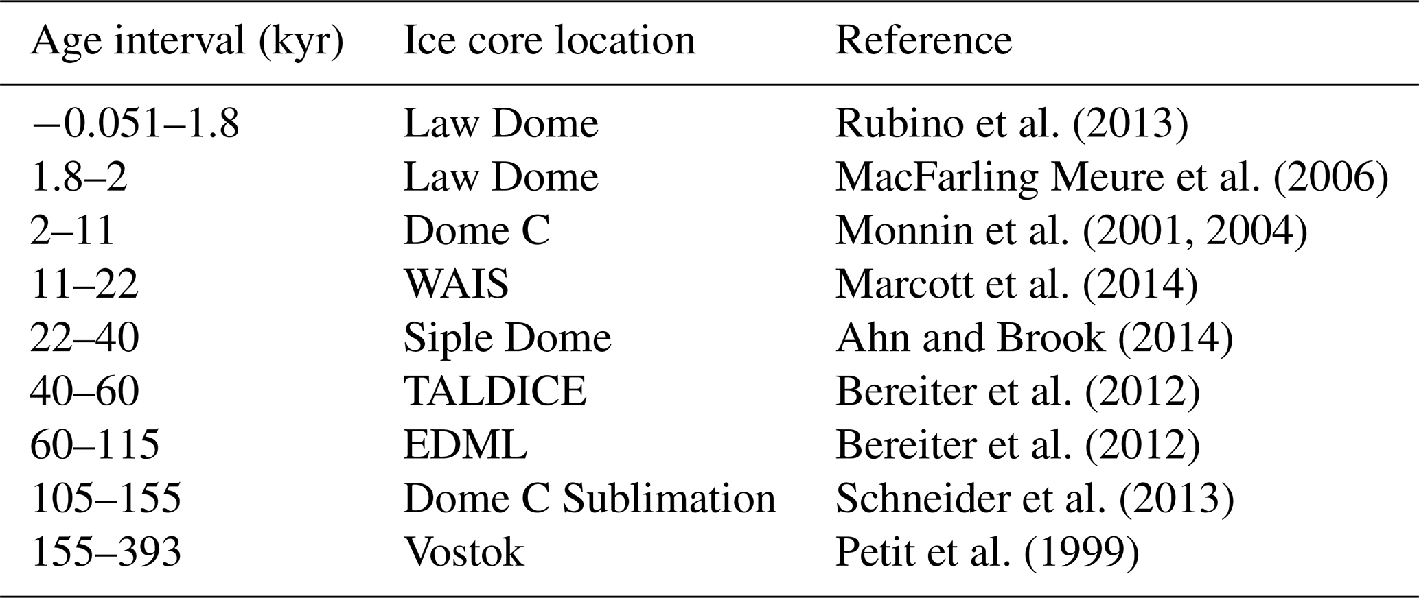
Table 1 Sources of ice core data used throughout, as compiled by Bereiter et al. (2015).

The ice cores record the pCO₂ of the Pleistocene glacial–interglacial cycles (Bereiter et al., 2015 and Table 1) and provide an opportunity for cross-calibrating proxy methods for determining atmospheric pCO₂ in the geological archive (${\mathrm{CO}}_{\mathrm{2}({\mathit{\epsilon }}_{\mathrm{p}}-\mathrm{alk})}$ and ${\mathrm{CO}}_{\mathrm{2}\left({\mathit{\delta }}^{\mathrm{11}}\mathrm{Bplank}\right)}$) with the direct-CO₂ measurements from the ice cores.

Study site

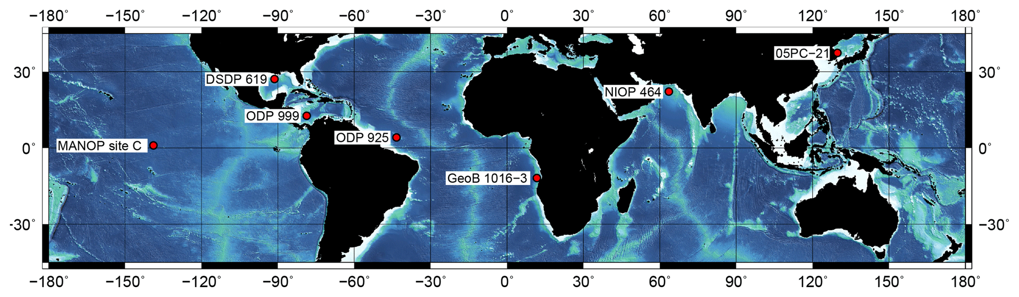
Ocean Drilling Program (ODP) Site 999 is located in the Caribbean Sea (12^∘44.639^′ N, 78^∘44.360^′ W; 2838 m water depth; Fig. 1), has an orbitally calibrated age model, and has been used previously for CO₂ reconstructions. Our temporal sampling resolution is ∼6 kyr in the Pleistocene and ∼9 kyr in the Pliocene. Although ${\mathrm{CO}}_{\mathrm{2}({\mathit{\epsilon }}_{\mathrm{p}}-\mathrm{alk})}$ and ${\mathrm{CO}}_{\mathrm{2}\left({\mathit{\delta }}^{\mathrm{11}}\mathrm{Bplank}\right)}$ are independent of one another in many respects, they both rely on assumptions about the equilibrium of surface seawater with the atmosphere with respect to CO₂, sea surface temperature, and on well-constrained age models, which can make direct comparison between records from different sites difficult. Here, we overcome these problems by producing ${\mathrm{CO}}_{\mathrm{2}({\mathit{\epsilon }}_{\mathrm{p}}-\mathrm{alk})}$ and ${\mathrm{CO}}_{\mathrm{2}\left({\mathit{\delta }}^{\mathrm{11}}\mathrm{Bplank}\right)}$ records from identical horizons in the same deep-ocean sediment core in (1) the late Pleistocene, permitting direct comparison to ice core data (Figs. 2a, 3), and (2) across the intensification of Northern Hemisphere glaciation (INHG) in the Pliocene (Seki et al., 2010; Martínez-Botí et al., 2015) (Fig. 2b).

Figure 1 Site map with locations of sites discussed the text.

In terms of CO₂, ODP Site 999 in the Caribbean Sea is today slightly out of equilibrium with the atmosphere, with surface waters a little oversaturated in CO₂, providing a small net source of CO₂ to the atmosphere (∼21 µatm; Takahashi et al., 2009). However, the site has been shown to be suitable for recording past changes in pCO₂ (Foster, 2008; Foster and Sexton, 2014) and the air–sea equilibrium is not thought to have changed significantly from the Pliocene to today (see discussion in Bartoli et al., 2011). It is one of few sites where both alkenone and boron isotope records can be acquired given the good preservation of both foraminifera and organic matter (Foster, 2008; Badger et al., 2013b; Foster and Sexton, 2014; Martínez-Botí et al., 2015), and Pliocene records of both are available (Bartoli et al., 2011; Badger et al., 2013b; Martínez-Botí et al., 2015). It also has been demonstrated previously to record glacial–interglacial cycles of pH ∕ CO₂ (Foster, 2008; Henehan et al., 2013) and a Pleistocene ${\mathrm{CO}}_{\mathrm{2}\left({\mathit{\delta }}^{\mathrm{11}}\mathrm{Bplank}\right)}$ record from 0 to 250 ka has been recently published (Chalk et al., 2017).

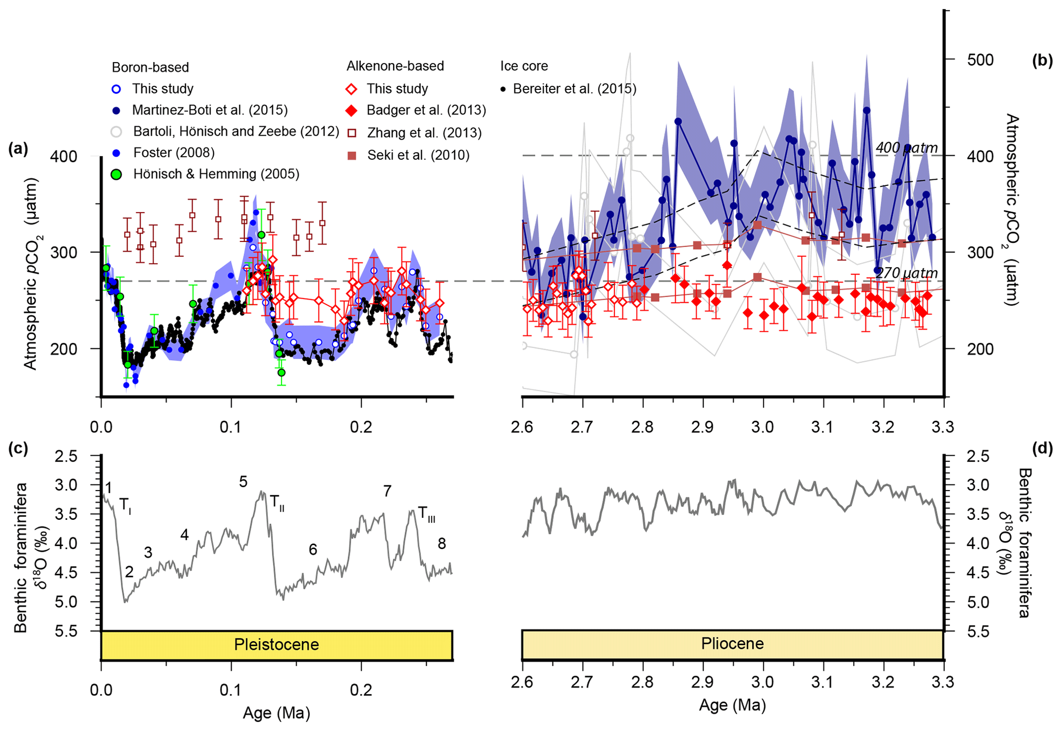
Figure 2 Atmospheric CO₂ reconstructions through the Plio-Pleistocene. (a) Published boron isotope ${\mathrm{CO}}_{\mathrm{2}\left({\mathit{\delta }}^{\mathrm{11}}\mathrm{Bplank}\right)}$ records from ODP Site 999: open blue circles (Chalk et al., 2017), filled bright blue circles (Foster, 2008; recalculated as described in the text), open grey circles (Bartoli et al., 2011), and filled dark blue circles (Martínez-Botí et al., 2015); and Deep Sea Drilling Project (DSDP) Site 668: filled green circles (Hönisch and Hemming, 2005). (b) Published ${\mathrm{CO}}_{\mathrm{2}({\mathit{\epsilon }}_{\mathrm{p}}-\mathrm{alk})}$ records from ODP Site 925: open maroon squares (Zhang et al., 2013); ODP Site 999: filled red diamonds (Badger et al., 2013a); and ice core records: filled black squares (Bereiter et al., 2015 and Table 1), as well as our new alkenone isotope records from ODP Site 999 (open red diamonds). The lith size-corrected (dashed black envelope) and uncorrected (solid red envelope) data of Seki et al. (2010) are also shown. All records are shown with 1σ uncertainties as described elsewhere. (c) The benthic foraminiferal stable oxygen isotope stack (Lisiecki and Raymo, 2005) with Marine Isotope Stage (MIS; numerals) and terminations (T) indicated.

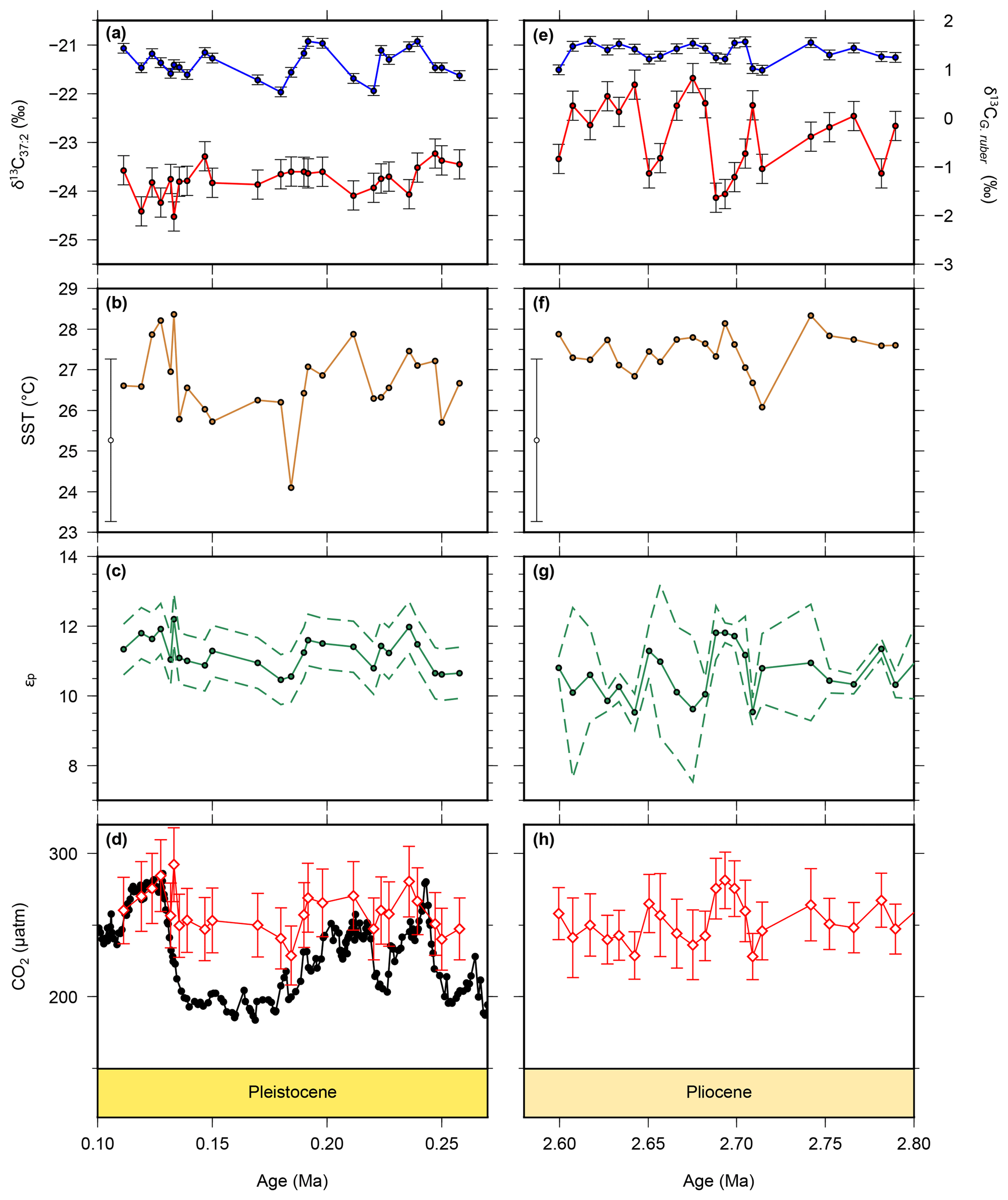
Figure 3 New and recalculated data for ${\mathrm{CO}}_{\mathrm{2}({\mathit{\epsilon }}_{\mathrm{p}}-\mathrm{alk})}$ for the Pleistocene and Pliocene from ODP Site 999. Alkenone δ¹³C values are shown as red circles for the Pleistocene (a) and Pliocene (b), with G. ruber δ¹³C from the same samples shown in blue. Alkenone unsaturation-derived SST is shown for the Pleistocene (b) and Pliocene (f). The Pliocene SST data have been previously published in Davis et al. (2013) and are from the same samples as our alkenone δ¹³C values. Calculated ε_p data are for the Pleistocene (c) and Pliocene (g) and atmospheric pCO₂ from ${\mathrm{CO}}_{\mathrm{2}({\mathit{\epsilon }}_{\mathrm{p}}-\mathrm{alk})}$ for the Pleistocene (d) and Pliocene (h) (red diamonds). Ice core pCO₂ data are shown for the Pleistocene (black circles) for comparison (Bereiter et al., 2015 and Table 1).

2 Methods

2.1 Alkenone isotopes

Our new alkenone-based CO₂ record was calculated following Badger et al. (2013b), with modern-day phosphate used in the estimation of the “b” term, $U_{\mathrm{37}}^{K{}^{\prime }}$' temperatures, and modern-day salinity (35 psu). Samples were freeze dried, ground to a fine powder by hand, and extracted by Soxhlet apparatus using a dichloromethane (DCM) ∕ methanol azeotrope (2:1, v∕v) refluxing for 24 h. Total lipid extracts were divided into three fractions (F) by small (4 cm) silica chromatography columns, with fractions eluting in 3 mL of n-hexane (F1), DCM (F2), and ethyl acetate ∕n-hexane (1:3, v:v, F3), respectively. Alkenones are eluted in F2. Alkenone identification was confirmed by gas chromatography (GC) mass spectrometry (ThermoQuest Trace MS, He carrier gas). Alkenone isotope analyses were performed using a Thermo Fisher Delta V connected via a GC isolink and ConFlo IV to a Trace GC. The GC oven was programmed to increase in temperature from 70 to 200 ^∘C at 20 ^∘C min⁻¹, then to 300 ^∘C at 6 ^∘C min⁻¹ and held isothermal for 25 min. Conversion to Vienna Pee Dee Belemnite (VPDB) was performed by reference to a laboratory standard gas of known δ¹³C and system performance was monitored using in-house fatty acid methyl ester and n-alkane standard mixtures of known isotopic composition. Long-term precision is approximately 0.3 ‰. To estimate sea surface temperature (SST), the F2 fraction was also analysed by GC-flame ionization detection (Hewlett Packard 5890 Series II), and the GC oven was programmed to increase in temperature from 70 to 130 ^∘C at 20 ^∘C min⁻¹, then to 300 ^∘C at 4 ^∘C min⁻¹ and held isothermal for 25 min. An approximately 50 m, 0.32 mm internal diameter capillary column with a 0.12 µm thick dimethylpolysiloxane equivalent film. A H₂ carrier gas was used, and quantification was monitored using a hexadecan-2-ol standard added prior to column chromatography. System performance as monitored with an in-house fatty acid methyl ester standard. Alkenone ratios were converted to SST using the global core-top calibration of Müller et al. (1998). Although this is a linear calibration, our uncertainty treatment (see below) should encompass any minor deviation from linear as $U_{\mathrm{37}}^{K{}^{\prime }}$ approaches 1 (see also the discussion in Badger et al., 2013b). All alkenone analyses were carried out at the Bristol node of the NERC Life Sciences Mass Spectrometry Facility hosted by the Organic Geochemistry Unit, University of Bristol.

The alkenone isotope δ¹³C value is used to calculate the total carbon isotope fractionation that occurs during algal growth (ε_p). This isotopic fractionation has been shown to be controlled by [CO_2(aq)] (Eq. 1; Jasper and Hayes, 1990) which can then be converted to atmospheric CO₂ using Henry's law.

$$\begin{array}{}\text{(1)}& {\displaystyle }{\mathit{\epsilon }}_{\mathrm{p}}={\mathit{\epsilon }}_{\mathrm{f}}-{\displaystyle \frac{b}{\left[{\mathrm{CO}}_{\mathrm{2}\left(\mathrm{aq}\right)}\right]}}\end{array}$$

To calculate ε_p from alkenone δ¹³C values, the carbon isotopic composition of dissolved inorganic carbon (DIC) is required; this is calculated from planktic foraminiferal calcite δ¹³C, whilst the fractionation which occurs during carbon fixation (ε_f) is assumed constant here. The b term is the sum of other physiological factors (such as growth rate, cell size, and light limitation) which is estimated from the relationship shown in the modern ocean between b and dissolved reactive phosphate $\left[{\mathrm{PO}}_{\mathrm{4}}^{\mathrm{3}-}\right]$ . Further details of the treatment are detailed in Badger et al. (2013b).

Error bars in relevant figures are all 1 SD and based on a full Monte Carlo propagation (n= 10 000) of the following uncertainties: ±2 ^∘C and ±0.1 ‰ were applied to temperature and foraminiferal calcite δ¹³C (normal probability function (pdf); 2σ error) and ±2 and ±0.1 to salinity and $\left[{\mathrm{PO}}_{\mathrm{4}}^{\mathrm{3}-}\right]$, respectively (2σ; uniform pdf). Uncertainties on alkenone δ¹³C were estimated from replicate runs and calcite δ¹³C from repeat runs of an internal standard. Integrated analytical and calibration uncertainties for alkenone-based temperatures were estimated and conservative estimates of likely variation for salinity and $\left[{\mathrm{PO}}_{\mathrm{4}}^{\mathrm{3}-}\right]$ were used. An 11 % error on the slope of b=a$\left[{\mathrm{PO}}_{\mathrm{4}}^{\mathrm{3}-}\right]$ +c was assumed, where a=116.96 and c=81.41 (Pagani et al., 1999).

For consistency with the ${\mathrm{CO}}_{\mathrm{2}\left({\mathit{\delta }}^{\mathrm{11}}\mathrm{Bplank}\right)}$ record for this site, we now adjust for the disequilibrium by subtracting the present-day CO₂ surplus and thus recalculate the included values of Badger et al. (2013b) accordingly. SSTs for our new Pliocene data were published in Davis et al. (2013).

2.2 Boron isotopes

Boron isotope data were published in Chalk et al. (2017) and are from the same core samples as our alkenone measurements. Globigerinoides ruber sensu stricto (white, n∼200 individuals from 300 to 355 µm) samples were measured for boron isotope composition on Thermo Scientific Neptune multicollector inductively coupled plasma mass spectrometer (MC-ICP-MS) at the University of Southampton according to methods described elsewhere (Rae et al., 2011; Foster et al., 2013; Martínez-Botí et al., 2015). Analytical uncertainty is given by the external reproducibility of repeat analyses of Japanese Geological Survey Porites coral standard (JCP) at the University of Southampton following Henehan et al. (2013) and is typically < 0.2 ‰ (at 95 % confidence). Metal element to calcium ratios (Li, Mg, B, Na, Al, Mn, Ba, Sr, Cd, U, Nd, and Fe) were analysed using an Thermo Element 2XR ICP-MS at the University of Southampton). Here, these data are used to assess adequacy of clay removal (Al ∕ Ca < 100 µmol mol⁻¹) and to generate down core temperature. pH and CO₂ were calculated using a Monte Carlo approach (uncertainties are 2 SD, n= 10 000 replicates) using R (R Core Team, 2015). For pH, we use a boron isotopic composition of seawater of 39.6 ‰ (2 SD of 0.1; Foster et al., 2010) and experimentally determined isotopic fractionation factor (1.027; Klochko et al., 2006), as well as the species-specific calibration for G. ruber of Henehan et al. (2013) (also with incorporated uncertainties). For the CO₂ calculations, we use a range of salinity (equal to that used in the ${\mathrm{CO}}_{\mathrm{2}({\mathit{\epsilon }}_{\mathrm{p}}-\mathrm{alk})}$ calculations) and total alkalinity (TA) that encompasses the modern values (34–37 and 2100–2500 µM, respectively, both with a uniform rather than normal probability distribution. Temperature was determined using Mg ∕ Ca of G. ruber following established methods; Delaney and Boyle, 1985; Evans and Müller, 2012). Mg ∕ Ca SST of planktic foraminifera is used for ${\mathrm{CO}}_{\mathrm{2}\left({\mathit{\delta }}^{\mathrm{11}}\mathrm{Bplank}\right)}$ and alkenone $U_{\mathrm{37}}^{K{}^{\prime }}$ for ${\mathrm{CO}}_{\mathrm{2}({\mathit{\epsilon }}_{\mathrm{p}}-\mathrm{alk})}$ so that the carrier organisms for the CO₂ reconstruction and SST measurements match, ensuring the temperature measurement is coming from the appropriate part of the water column. Inorganic chemical constants were used from the seacarb package in R (Gattuso et al., 2015) and using published values for the p$K_{\text{B}}^{*}$ (dissociation constant for boric acid) (Dickson, 1990). Reconstructed atmospheric CO₂ values from Foster (2008) were recalculated to match this approach. All uncertainties are included in our simulation and are roughly equivalent to those assumed for the alkenone data and are exactly the same as those used for Martinez-Boti et al. (2015), excluding the δ¹¹B_sw, thus providing a fair comparison.

2.3 Coccolith length measurements

The uptake of CO₂ into the coccolithophore cell is affected by the cell size and geometry; using alkenones limits the variation of cell geometry by restricting the source organism to one with exclusively spherical cells (Laws et al., 1997; Popp et al., 1998), but some change in cell size is possible. Coccolith size is used as an semi-quantitative proxy for cell size because coccolith size is typically larger on larger cells, with that relationship being broadly consistent within a single taxonomic group where growth behaviour is broadly comparable (Henderiks, 2008; Gibbs et al., 2013; Sheward et al., 2017). Long-axis coccolith length measurements were therefore taken from 100 specimens of the family Noelaerhabdaceae per sample from standard smear slides. Specimens were imaged at 1500× magnification and measured using CellD software.

To investigate the potential influence of changing cell size on ${\mathrm{CO}}_{\mathrm{2}({\mathit{\epsilon }}_{\mathrm{p}}-\mathrm{alk})}$, Eq. (1) can be adapted:

$$\begin{array}{}\text{(2)}& {\displaystyle }{\mathit{\epsilon }}_{\mathrm{p}}={\mathit{\epsilon }}_{\mathrm{f}}-{\displaystyle \frac{b^{\prime }}{\left[{\mathrm{CO}}_{\mathrm{2}\left(\mathrm{aq}\right)}\right]}}.\end{array}$$

with b^′ calculated from using the volume to surface area ratio (V : SA) of modern and fossil coccospheres (Eq. 3; Henderiks and Pagani, 2007):

$$\begin{array}{}\text{(3)}& {\displaystyle }{b}^{\prime }=b{\displaystyle \frac{\mathrm{V}:{\mathrm{SA}}_{\mathrm{fossil}}}{\mathrm{V}:{\mathrm{SA}}_{\mathrm{Ehux}}}}.\end{array}$$

V : SA_Ehux is 0.9±0.1 µm in modern haptophytes (Popp et al., 1998) and V : SA_fossil can be estimated from lith size measurements (Eq. 4; Henderiks and Pagani, 2007):

$$\begin{array}{}\text{(4)}& {\displaystyle }{D}_{\mathrm{cell}}=\mathrm{0.55}+\mathrm{0.88}{L}_{\mathrm{coccolith}}.\end{array}$$

2.4 Age model

For the 0–500 ka interval, we generated a detailed age model by tuning the planktic foraminifer (G. ruber) δ¹⁸O record from Site 999 (at ∼0.5 to 2.0 kyr resolution) (Schmidt et al., 2006) to the LR04 benthic δ¹⁸O stack (Lisiecki and Raymo, 2005) using the AnalySeries software (Paillard et al., 1996). The Pliocene portion of Site 999 is part the LR04 stack and that astronomically tuned age model is used here (Lisiecki and Raymo, 2005).

2.5 Bayesian exploration of ${\mathrm{CO}}_{\mathrm{2}({\mathit{\epsilon }}_{\mathrm{p}}-\mathrm{alk})}$ input variables

In order to examine the influence of the various input parameters for the calculation of pCO₂ from alkenone δ¹³C values, we carry out a second set of Monte Carlo simulations (n= 100 000) with expanded uncertainty. In this case, we more fully explore uncertainty space using the following input uncertainties (at 95 % confidence or full range): SST (normal distribution, ±6 ^∘C), ε_f (uniform distribution, 24 to 28), b (normal distribution, ±40), and CO₂ disequilibrium (20±20). These input distributions are our prior distributions. We then evaluate the CO₂ output for each alkenone sample against synchronous ice core pCO₂ and boron isotope pCO₂ for the Pleistocene and Pliocene, respectively. By only selecting those simulated alkenone pCO₂ levels that agree with ice core or p${\mathrm{CO}}_{\mathrm{2}\left({\mathit{\delta }}^{\mathrm{11}}\mathrm{Bplank}\right)}$ (including associated uncertainties), we can reevaluate the input distributions (our posterior) and gain insights into the relative importance of each of the input variables in potentially driving the observed disagreement in pCO₂. Uncertainties in the p${\mathrm{CO}}_{\mathrm{2}\left({\mathit{\delta }}^{\mathrm{11}}\mathrm{Bplank}\right)}$ are as described above, and we apply an uncertainty of ±6 ppm (2 s) for the ice core pCO₂ record (Ahn et al., 2012).

3 Results and discussion

Alkenone and G. ruber δ¹³C values (Fig. 3a, e) were used to calculate ε_p values (Fig. 3c, g). Alkenone δ¹³C values are relatively stable through the Pleistocene portion of the record, varying between −24.5 ‰ and −23.2 ‰. Values are slightly higher in the Pliocene, varying between −24.1 ‰ and −21.7 ‰. G. ruber δ¹³C values are relatively stable through the whole record, varying between 0.53 ‰ and 1.57 ‰. These give rise to ε_p values which are similarly fairly stable, varying between 10.5 ‰ and 12.2 ‰ in the Pleistocene, and between 9.53 ‰ and 11.8 ‰ in the Pliocene. Our $U_{\mathrm{37}}^{K{}^{\prime }}$ SST (Fig. 3c, g) record shows warmer temperatures in the Pliocene of around 27 ^∘C, with cooler temperatures recorded in the Pleistocene, with the coldest SST recorded in the glacial which is ∼2 ^∘C cooler than the interglacial. These records are combined (see methods section) to produce the pCO₂ record (Figs. 2, 3c, f), which shows largely stable and invariant values through both the Pliocene and Pleistocene portions of our record.

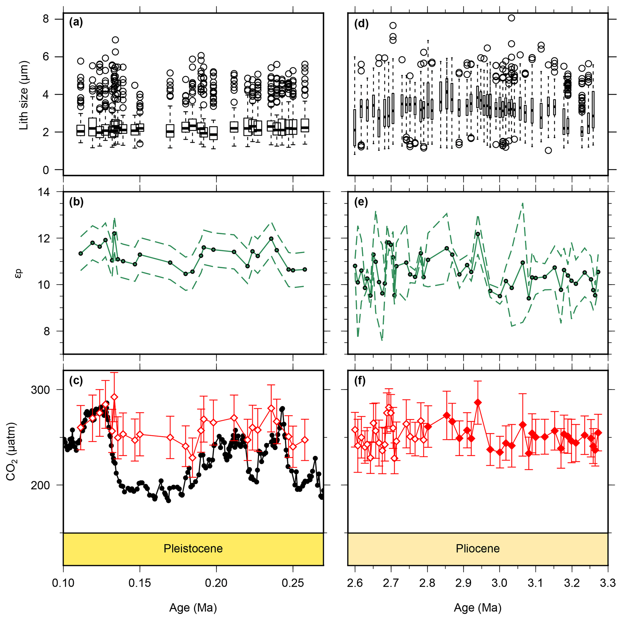
Figure 4 Lith size data for samples used for CO₂ calculations. Pleistocene lith size (a) are from this study, whilst Pliocene (b) values were published previously (Davis et al., 2013) but are from the same samples as our CO₂ estimates. Pleistocene ε_p (b) are from this study, whilst the Pliocene data are from this study (2.6–2.8 Ma) and from Badger et al. (2013b) (2.8–3.3 Ma). The lower panels show ${\mathrm{CO}}_{\mathrm{2}({\mathit{\epsilon }}_{\mathrm{p}}-\mathrm{alk})}$ for the Pleistocene (c) and Pliocene (f) as red diamonds. The filled diamonds in panel (f) are from Badger et al. (2013b). The Pleistocene ice core data (Bereiter et al., 2015 and Table 1) are shown for comparison in panel (c). The drop in lith size from the Pliocene to Pleistocene is similar to what has been documented previously (Young, 1990). Outliers in panels (a) and (d) were calculated following the 1.5 rule in R (R Core Team, 2015).

Published low temporal resolution Pliocene records from Site 999 (Seki et al., 2010), using both the ${\mathrm{CO}}_{\mathrm{2}({\mathit{\epsilon }}_{\mathrm{p}}-\mathrm{alk})}$ and ${\mathrm{CO}}_{\mathrm{2}\left({\mathit{\delta }}^{\mathrm{11}}\mathrm{Bplank}\right)}$ palaeobarometers, show a pCO₂ decrease at ∼2.8 Ma. However, this agreement relies on correcting the ${\mathrm{CO}}_{\mathrm{2}({\mathit{\epsilon }}_{\mathrm{p}}-\mathrm{alk})}$ for changes in haptophyte cell size, which was based on a low temporal resolution lith size record (Seki et al., 2010). Changes in haptophyte cell size alter the volume to surface area ratio available for gaseous exchange and can therefore modify the fractionation recorded by ${\mathrm{CO}}_{\mathrm{2}({\mathit{\epsilon }}_{\mathrm{p}}-\mathrm{alk})}$ (Popp et al., 1998). Our new ${\mathrm{CO}}_{\mathrm{2}({\mathit{\epsilon }}_{\mathrm{p}}-\mathrm{alk})}$ record at Site 999 now spans 3.3–2.6 Ma at higher temporal resolution, supplementing data from Badger et al. (2013b). A lith size record has also been generated for the same samples used for ${\mathrm{CO}}_{\mathrm{2}({\mathit{\epsilon }}_{\mathrm{p}}-\mathrm{alk})}$ for 3.3–2.6 Ma (Davis et al., 2013). We find no evidence to support the change in lith size applied by Seki et al. (2010) with lith size (and hence cell size) remaining stable across the primary pCO₂ change at 2.8 Ma (Davis et al., 2013). Consequently, although our new ${\mathrm{CO}}_{\mathrm{2}({\mathit{\epsilon }}_{\mathrm{p}}-\mathrm{alk})}$ record is of higher resolution than that of Seki et al. (2010), we no longer have any evidence for the cell size shift at 2.7 Ma (Fig. 4).

We compare our record with the ${\mathrm{CO}}_{\mathrm{2}\left({\mathit{\delta }}^{\mathrm{11}}\mathrm{Bplank}\right)}$ records of Martínez-Botí et al. (2015) in Fig. 2. With the cell size correction now removed, the decrease in ${\mathrm{CO}}_{\mathrm{2}({\mathit{\epsilon }}_{\mathrm{p}}-\mathrm{alk})}$ across the INHG, and the agreement of ${\mathrm{CO}}_{\mathrm{2}({\mathit{\epsilon }}_{\mathrm{p}}-\mathrm{alk})}$ with ${\mathrm{CO}}_{\mathrm{2}\left({\mathit{\delta }}^{\mathrm{11}}\mathrm{Bplank}\right)}$, both now disappear (red symbols, Fig. 2b). As such, ${\mathrm{CO}}_{\mathrm{2}({\mathit{\epsilon }}_{\mathrm{p}}-\mathrm{alk})}$ for this whole Pliocene interval (2.6–3.3 Ma) remains stable and low (mean ${\mathrm{CO}}_{\mathrm{2}({\mathit{\epsilon }}_{\mathrm{p}}-\mathrm{alk})}$ $=\mathrm{251}\pm \mathrm{13}$; 1σ min =228,  max =286 µatm), whereas ${\mathrm{CO}}_{\mathrm{2}\left({\mathit{\delta }}^{\mathrm{11}}\mathrm{Bplank}\right)}$ is on average higher and more variable (mean ${\mathrm{CO}}_{\mathrm{2}\left({\mathit{\delta }}^{\mathrm{11}}\mathrm{Bplank}\right)}$ $=\mathrm{342}\pm \mathrm{50}$; 1σ min =234, max =452 µatm).

In the Pleistocene, our ${\mathrm{CO}}_{\mathrm{2}({\mathit{\epsilon }}_{\mathrm{p}}-\mathrm{alk})}$ record covers one complete glacial–interglacial (G-IG) cycle from 110 to 260 ka, encompassing MIS5–7, and the end of MIS8, and terminations II and III (open red diamonds; Fig. 2a). The ${\mathrm{CO}}_{\mathrm{2}\left({\mathit{\delta }}^{\mathrm{11}}\mathrm{Bplank}\right)}$ record of Chalk et al. (2017) covers two G-IG cycles from the late Holocene to MIS8 (open blue circles; Fig. 2a). δ¹¹B_plank closely tracks the rise and fall of pCO₂ derived from ice cores (Chalk et al., 2017), with ${\mathrm{CO}}_{\mathrm{2}\left({\mathit{\delta }}^{\mathrm{11}}\mathrm{Bplank}\right)}$ exhibiting similar values to atmospheric CO₂ within uncertainty (Fig. 2a), and with only small deviations from ice core CO₂ as a result of (i) the noise in the reconstruction and (ii) perhaps a small diagenetic effect on ${\mathrm{CO}}_{\mathrm{2}\left({\mathit{\delta }}^{\mathrm{11}}\mathrm{Bplank}\right)}$ relating to periods of carbonate dissolution in portions of the core which show high foraminiferal fragmentation (e.g., MIS5d; Schmidt et al., 2006).

In contrast, ${\mathrm{CO}}_{\mathrm{2}({\mathit{\epsilon }}_{\mathrm{p}}-\mathrm{alk})}$ is within error of the ice core data only during the interglacials when CO₂ partial pressures are similar to those of the pre-industrial era. Crucially, ${\mathrm{CO}}_{\mathrm{2}({\mathit{\epsilon }}_{\mathrm{p}}-\mathrm{alk})}$ clearly fails to record the lower pCO₂ of the glacials, remaining at around 260 µatm throughout (mean ${\mathrm{CO}}_{\mathrm{2}({\mathit{\epsilon }}_{\mathrm{p}}-\mathrm{alk})}$ $=\mathrm{259}\pm \mathrm{27}$; Fig. 2a). This concentration of pCO₂ is also very close to that recorded by ${\mathrm{CO}}_{\mathrm{2}({\mathit{\epsilon }}_{\mathrm{p}}-\mathrm{alk})}$ in the Pliocene at this site (mean ${\mathrm{CO}}_{\mathrm{2}({\mathit{\epsilon }}_{\mathrm{p}}-\mathrm{alk})}$ $=\mathrm{252}\pm \mathrm{26}$ µatm; Fig. 2). Similar alkenone behaviour has also been observed in another, albeit lower-resolution, record from ODP Site 925 (Zhang et al., 2013; Fig. 2), where the ${\mathrm{CO}}_{\mathrm{2}({\mathit{\epsilon }}_{\mathrm{p}}-\mathrm{alk})}$ remains unchanged during the Pleistocene (20–170 ka) and Pliocene.

Overall, these results suggest that, at least at these sites, the ${\mathrm{CO}}_{\mathrm{2}\left({\mathit{\delta }}^{\mathrm{11}}\mathrm{Bplank}\right)}$ palaeobarometer does faithfully record atmospheric CO₂ change, whereas the ${\mathrm{CO}}_{\mathrm{2}({\mathit{\epsilon }}_{\mathrm{p}}-\mathrm{alk})}$ proxy is unable to reconstruct the low levels of atmospheric CO₂ during the glacial. This suggests that, in its present and frequently applied form, ${\mathrm{CO}}_{\mathrm{2}({\mathit{\epsilon }}_{\mathrm{p}}-\mathrm{alk})}$ is not accurately recording atmospheric CO₂, and this could explain the discrepancy between the Pliocene ${\mathrm{CO}}_{\mathrm{2}({\mathit{\epsilon }}_{\mathrm{p}}-\mathrm{alk})}$ and ${\mathrm{CO}}_{\mathrm{2}\left({\mathit{\delta }}^{\mathrm{11}}\mathrm{Bplank}\right)}$ records. We further evaluate this by using regression analysis between ice core and the paired-proxy data (Fig. 5). ${\mathrm{CO}}_{\mathrm{2}\left({\mathit{\delta }}^{\mathrm{11}}\mathrm{Bplank}\right)}$ levels are largely consistent with those determined from ice cores, clustering around the 1:1 line with a slope also close to 1 (0.95±0.13) (Fig. 5a), whereas variance in ${\mathrm{CO}}_{\mathrm{2}({\mathit{\epsilon }}_{\mathrm{p}}-\mathrm{alk})}$ is strongly muted compared to that observed in the ice core data (Fig. 5b).

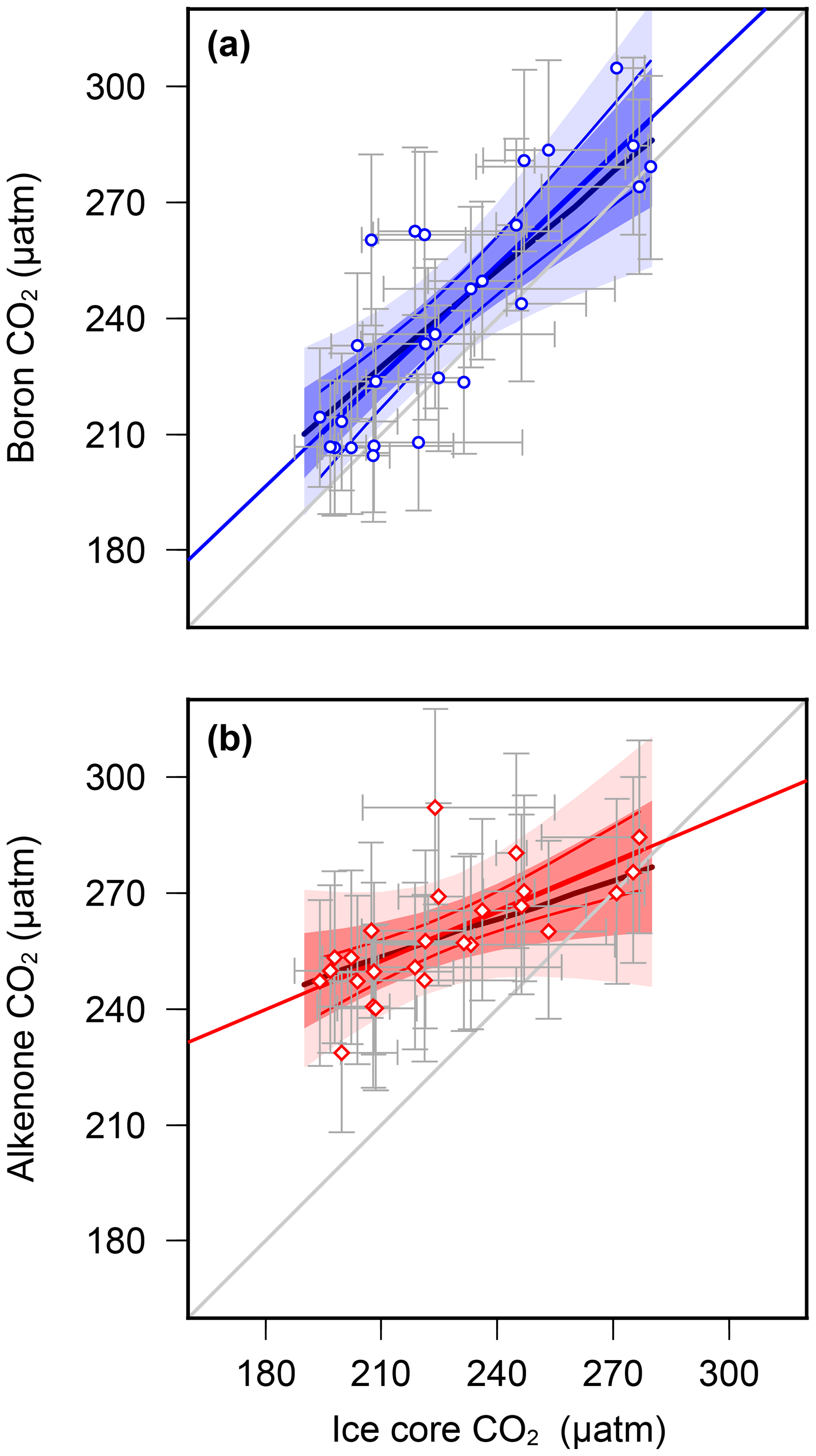
Figure 5 Regression analyses of proxy-based pCO₂ with ice core data (a) ${\mathrm{CO}}_{\mathrm{2}\left({\mathit{\delta }}^{\mathrm{11}}\mathrm{Bplank}\right)}$ (Chalk et al., 2017) and (b) ${\mathrm{CO}}_{\mathrm{2}({\mathit{\epsilon }}_{\mathrm{p}}-\mathrm{alk})}$ vs. ice core data (Bereiter et al., 2015 and Table 1) for MIS5–8, interpolated in the age domain. Regression lines (in red/blue) are linear fits with 68 % and 95 % confidence intervals, calculated by bootstrapping the uncertainties in proxy pCO₂ (Monte Carlo method described in the methods section). Uncertainty in the ice core values is by estimated by applying a 3000 uncertainty in the age model during interpolation. Uncertainty envelopes considering data points alone (no bootstrap) are solid lines, with p_max regressions in the thicker, darker colours. A 1:1 line is shown in grey for comparison. Statistical calculations were performed in R (R Core Team, 2015).

As both cell size (Popp et al., 1998) and growth rate (Bidigare et al., 1997) can modify δ¹³C_alk via the b term, we investigated whether either of these could explain the muted response of ${\mathrm{CO}}_{\mathrm{2}({\mathit{\epsilon }}_{\mathrm{p}}-\mathrm{alk})}$ to atmospheric CO₂. Haptophyte cell size can be estimated from their lith size, but as noted above, there is no evidence for significant changes in the Pliocene (Davis et al., 2013) nor is there evidence for any change across MIS5–8 (Fig. 4a). There is an overall reduction in mean lith size from the Pliocene to the Pleistocene (Fig. 4a, b), which could offset a long-term pCO₂ decline and thus explain the apparent lack of difference between Pliocene and Pleistocene ${\mathrm{CO}}_{\mathrm{2}({\mathit{\epsilon }}_{\mathrm{p}}-\mathrm{alk})}$ at Site 999 (Fig. 6). However, this longer-term reduction in lith size cannot explain the muted response to Pleistocene G-IG CO₂ change.

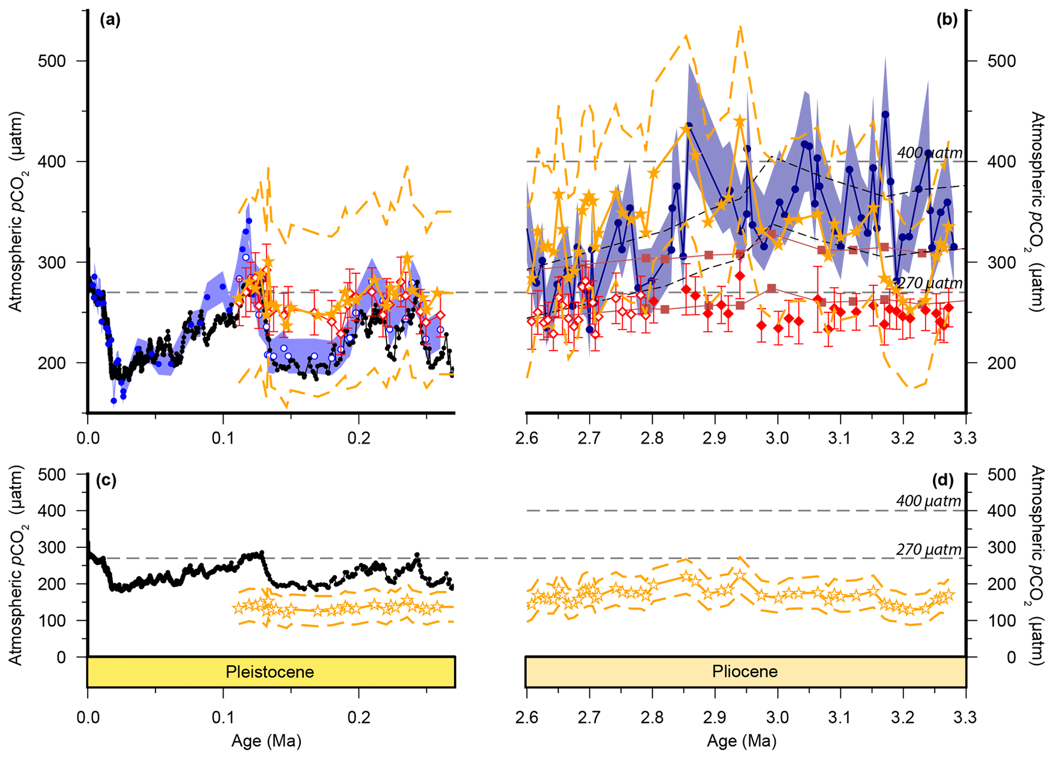
Figure 6 Cell size corrections to ${\mathrm{CO}}_{\mathrm{2}({\mathit{\epsilon }}_{\mathrm{p}}-\mathrm{alk})}$. Ornamentation is the same as Fig. 1, with the addition of cell-size-corrected ${\mathrm{CO}}_{\mathrm{2}({\mathit{\epsilon }}_{\mathrm{p}}-\mathrm{alk})}$. The smaller liths than modern E. huxleyii across all of our records mean that a direct application of the method of Henderiks and Pagani (2007) results in substantially lower ${\mathrm{CO}}_{\mathrm{2}({\mathit{\epsilon }}_{\mathrm{p}}-\mathrm{alk})}$ throughout (open orange stars; c, d). As the main interest is in the effect of the Plio-Pleistocene change in cell size we observe, we adjusted the b^′ term so that ${\mathrm{CO}}_{\mathrm{2}({\mathit{\epsilon }}_{\mathrm{p}}-\mathrm{alk})}$ matched our uncorrected ${\mathrm{CO}}_{\mathrm{2}({\mathit{\epsilon }}_{\mathrm{p}}-\mathrm{alk})}$ record during the last interglacial (filled orange stars; a, b).

Growth rate is more difficult to reconstruct; most available proxy systems reconstruct phytoplankton or whole ecosystem productivity, rather than coccolithophorid growth rate. However, emerging trace metal datasets do suggest changing productivity on glacial–interglacial timescales at Site 999, with lower productivity in the glacial (Trumbo, 2015). If lower productivity is linked with a simultaneous reduction in growth rate, then it could explain some of the lack of signal in ${\mathrm{CO}}_{\mathrm{2}({\mathit{\epsilon }}_{\mathrm{p}}-\mathrm{alk})}$; however, to reduce the ${\mathrm{CO}}_{\mathrm{2}({\mathit{\epsilon }}_{\mathrm{p}}-\mathrm{alk})}$ sufficiently to overlap with ice core CO₂ would require an order of magnitude reduction in growth rates during the glacial. This suggests that either our understanding of growth rate effects on ${\mathrm{CO}}_{\mathrm{2}({\mathit{\epsilon }}_{\mathrm{p}}-\mathrm{alk})}$ is incorrect, or the estimation of cell size using preserved liths does not capture original cell size variations, or a combination of these or other factors leads to the rather muted trends in ${\mathrm{CO}}_{\mathrm{2}({\mathit{\epsilon }}_{\mathrm{p}}-\mathrm{alk})}$ through the glacial–interglacial cycle.

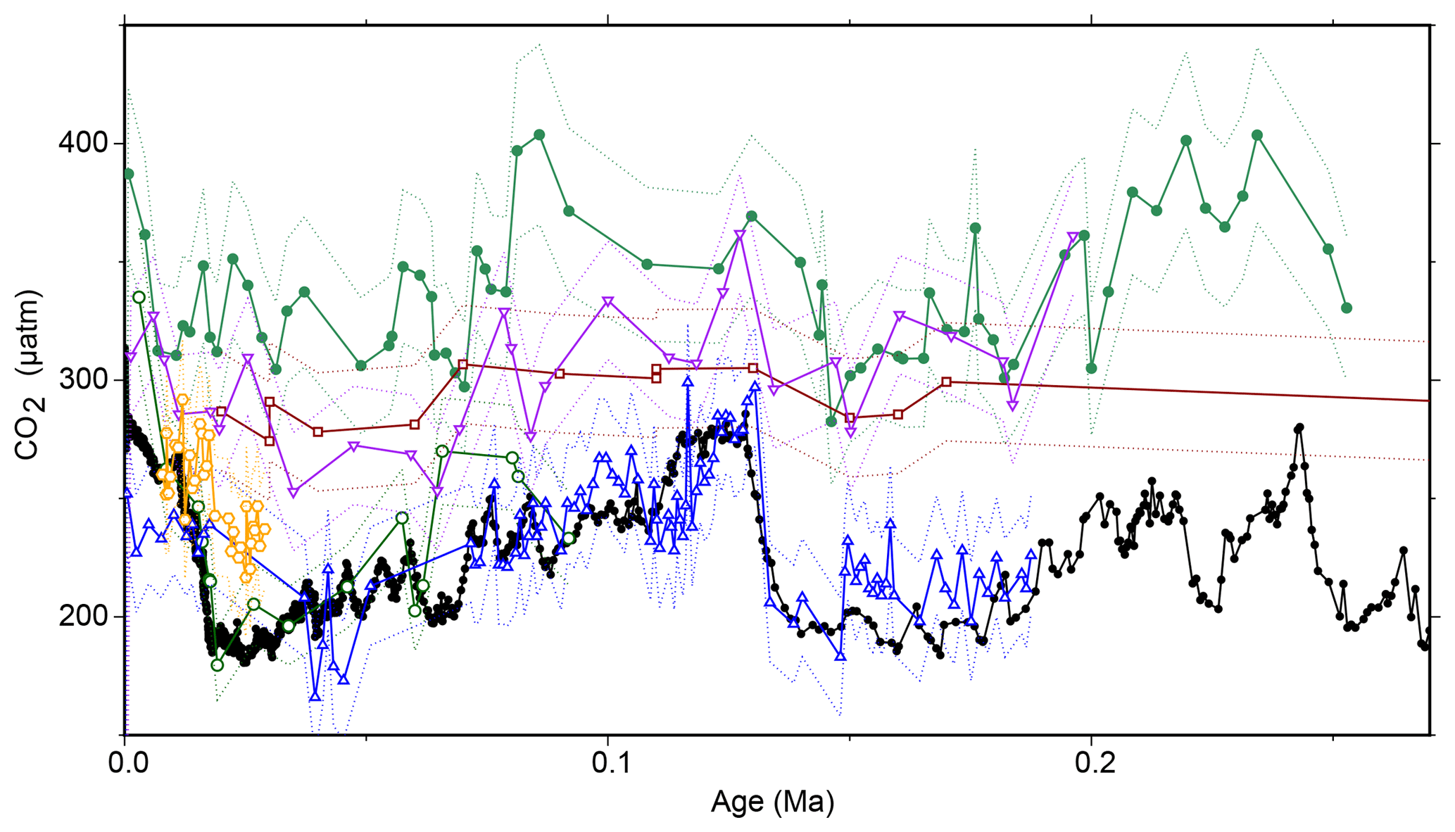
Figure 7 Recalculated ${\mathrm{CO}}_{\mathrm{2}({\mathit{\epsilon }}_{\mathrm{p}}-\mathrm{alk})}$. Previous work (Jasper and Hayes, 1990; Jasper et al., 1994) calculated ${\mathrm{CO}}_{\mathrm{2}({\mathit{\epsilon }}_{\mathrm{p}}-\mathrm{alk})}$ using a different model; here, we recalculate the earlier work using the modern methodology and Monte Carlo propagation applied to our other sites. All previous records have been recalculated using the same methodology as our new record, with some corrections and adjustments (for example, for growth rate or lith size) removed to allow direct comparisons. Records are from MANOP site C from the central equatorial Pacific (0^∘57.2^′ N, 138^∘57.3^′ W; filled green circles; Jasper et al., 1994), DSDP Site 619 in the Pigmy Basin, northern Gulf of Mexico (27^∘11.6^′ N, 91^∘24.5^′ W; open green circles; Jasper and Hayes, 1990), site 05PC-21 from the Sea of Japan (38.40^∘ N, 131.55 ^∘ E; open blue triangles; Bae et al., 2015), site NIOP464 in the Arabian Sea (22.15^∘ N, 63.35^∘ E; open orange hexagons; Palmer et al., 2010), site GeoB 1016-3 in the Angola Current (11.59^∘ S, 11.70^∘ E; inverted purple triangles; Andersen et al., 1999), and ODP Site 925 (4^∘12.25^′ N, 43^∘29.33^′ W; open dark red squares; Zhang et al., 2013). Ice core data are shown as filled black circles and lines (Bereiter et al., 2015 and Table 1). Dashed lines are 2σ uncertainties from Monte Carlo error propagation as described elsewhere in the text.

The failure of ${\mathrm{CO}}_{\mathrm{2}({\mathit{\epsilon }}_{\mathrm{p}}-\mathrm{alk})}$ from these two sites to record the G-IG pCO₂ variation also necessitates reassessment of earlier ${\mathrm{CO}}_{\mathrm{2}({\mathit{\epsilon }}_{\mathrm{p}}-\mathrm{alk})}$ studies that were able to reconstruct such changes. For instance, whilst Jasper and Hayes (1990) replicated the CO₂ change over the last 100 kyr of the Vostok ice core from Deep Sea Drilling Project (DSDP) Site 619 (Gulf of Mexico) and Bae et al. (2015) are able to replicate the ice core data at a site in the Sea of Japan, records from the Arabian Sea (Palmer et al., 2010), Angola Current (Andersen et al., 1999), and the equatorial Atlantic (Zhang et al., 2013) either fail to record ice core CO₂ or require additional corrections to do so (Fig. 7). It may also be that at some sites, such as at equatorial Pacific MANOP (Manganese Nodule Project) site C (Figs. 1, 7), these records represent changing air–sea disequilibrium (Jasper et al., 1994). Two of these studies interpreted their data using a different ε_p relationship than later work; when these data are recalculated using the more recent model, the patterns remain unchanged (Fig. 7). What is more, in a global alkenone δ¹³C calibration study (Pagani et al., 2002) aimed at replicating Holocene atmospheric conditions, it was noted that low-latitude (subtropical) sites perform poorly, consistent with our observations. Considering this present study and previously published work, five out of seven late Pleistocene alkenone δ¹³C studies do not show the variations in pCO₂ evident from contemporaneous ice core records (Figs. 2, 7).

Our Bayesian approach allows us to explore the ${\mathrm{CO}}_{\mathrm{2}({\mathit{\epsilon }}_{\mathrm{p}}-\mathrm{alk})}$ proxy, as it was mathematically expressed by Bidigare et al. (1997) and subsequent authors, and test which variables may be responsible for causing the observed disagreement with the ice core and ${\mathrm{CO}}_{\mathrm{2}\left({\mathit{\delta }}^{\mathrm{11}}\mathrm{Bplank}\right)}$ records given a largely invariant ε_p for the Pleistocene. Figure 8 illustrates the prior distributions of the input variables (blue) and an example posterior for the alkenone sample at 150 ka (red). As can be seen in this example, selecting only those simulations of ${\mathrm{CO}}_{\mathrm{2}({\mathit{\epsilon }}_{\mathrm{p}}-\mathrm{alk})}$ that overlap with the ice core CO₂ for this time interval shifts the distributions such that an agreement is found when b is lower than the prior, ε_f tends to be higher than the prior, and SST and CO₂ disequilibrium are little different. Figure 9 shows the posterior median and 95 % distribution of b, ε_f, and SST for all the samples from the Pleistocene and Pliocene in time series. Patterns that emerge are illustrated in Fig. 10, where a negative relationship between pCO₂ and posterior ε_f and a positive relationship between pCO₂ and posterior b and SST are evident. For SST, it should also be noted that for the Pleistocene the posterior correlates well with the prior, while for the Pliocene it is significantly elevated (Fig. 10), perhaps suggesting a role for incorrect SST in driving some of the lack of Pliocene to Pleistocene change in ${\mathrm{CO}}_{\mathrm{2}({\mathit{\epsilon }}_{\mathrm{p}}-\mathrm{alk})}$ observed (Fig. 2). This SST change would however need to be substantial and go beyond the ±2 ^∘C we include in our uncertainty propagation, and would also potentially influence ${\mathrm{CO}}_{\mathrm{2}\left({\mathit{\delta }}^{\mathrm{11}}\mathrm{Bplank}\right)}$, further complicating this finding.

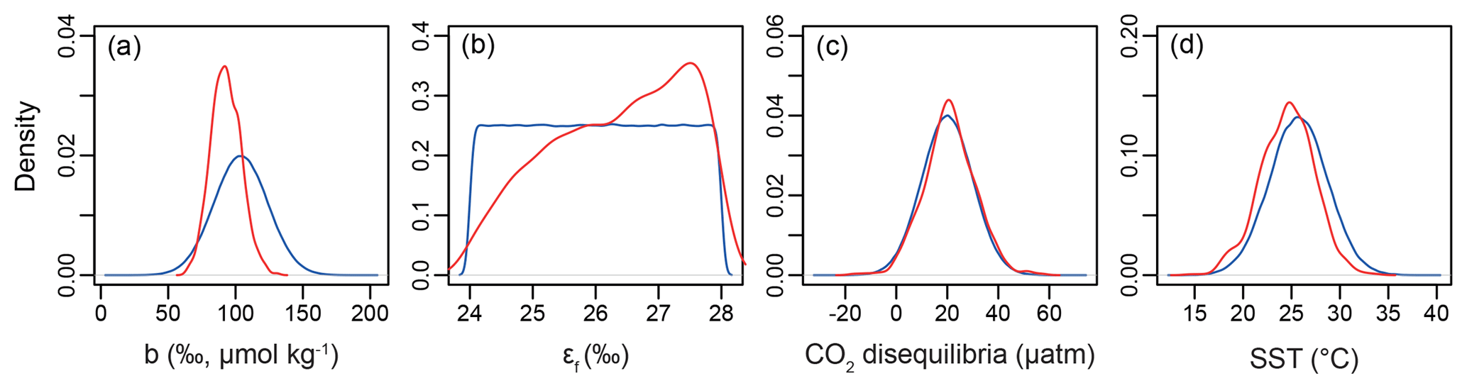
Figure 8 Example of the Bayesian treatment of the ${\mathrm{CO}}_{\mathrm{2}({\mathit{\epsilon }}_{\mathrm{p}}-\mathrm{alk})}$ proxy; the sample shown is 0.15 Ma from ODP Site 999. In all panels, the prior is shown in blue and the posterior in red. (a) The b term, (b) ε_f, (c) the extent of CO₂ disequilibria, and (d) sea surface temperature.

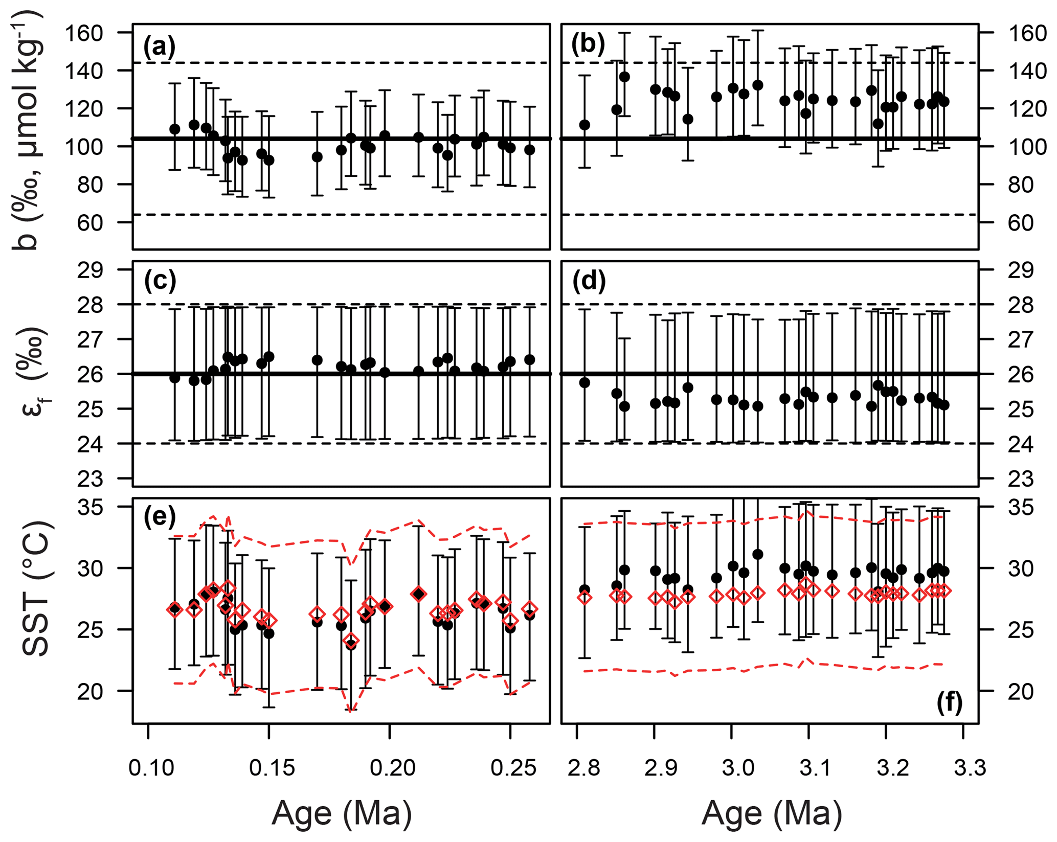
Figure 9 Time series of priors and posteriors for the b term (a, b), ε_f (c, d), and SST (e, f). The Pleistocene is shown on the panels on the left and the Pliocene on the right. In panels (a–d), the mean of the prior distribution is shown as a thick black line. For the b term, 95 % of the input distribution is shown as a dotted line; for ε,_f the total range is shown. See Fig. 7 for examples of these distributions as probability functions. For SST (e, f), the prior is shown as red diamonds, with 95 % of the distribution shown as the dashed lines. In all panels, the medians of the posterior distributions are shown as circles, with error bars encompassing 95 % of the range.

We recognize that the nature of the patterns we observe here is a function somewhat of the range used for each input term. The chosen ranges are however conservative, but realistic, assessments of the likely uncertainty associated with each term. For instance, b±40 encompasses the residual scatter around the relationship between b and [PO₄] described by Pagani et al. (2005). In addition to pointing towards a potential underestimate of Pliocene SST with the $U_{\mathrm{37}}^{K{}^{\prime }}$ proxy at ODP 999, this Bayesian treatment supports the assertion that the current understanding of the ${\mathrm{CO}}_{\mathrm{2}({\mathit{\epsilon }}_{\mathrm{p}}-\mathrm{alk})}$ proxy is wanting and that the b term may not in fact capture the scaling of the relevant physiological parameters or those that are truly important. In particular, it appears that the physiological parameters packaged in the b term, and potentially the degree of fractionation upon fixation, ε_f, are themselves a function of CO₂ or some parameter that correlates with CO₂ (e.g., temperature, nutrients, growth rate).

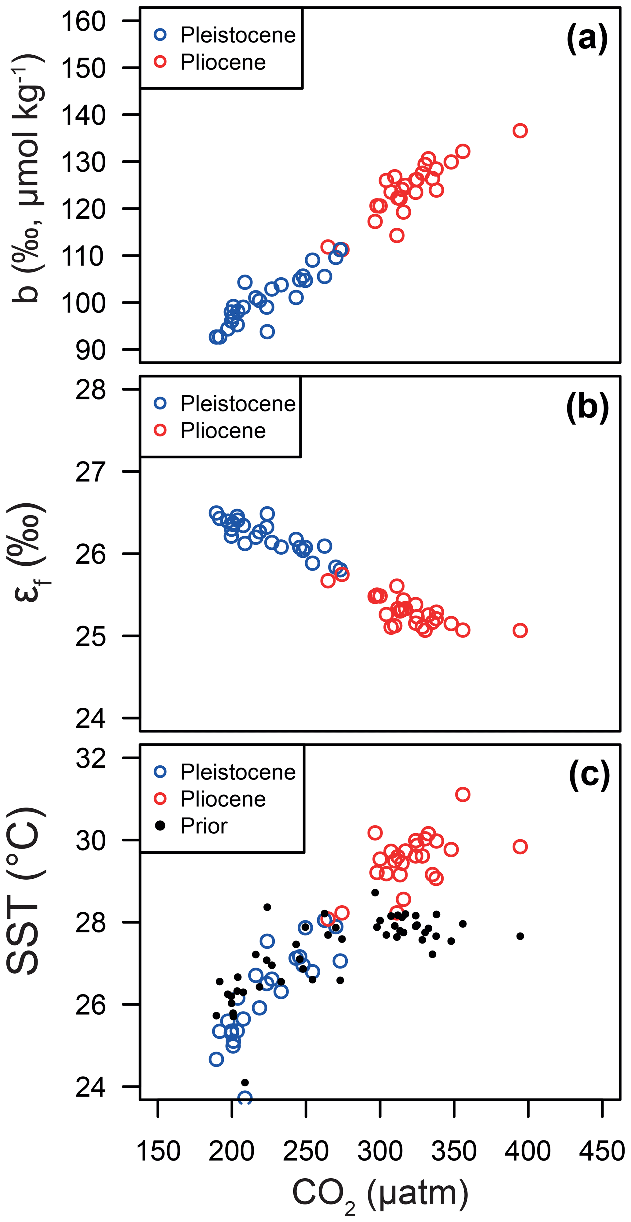
Figure 10 Relationships between CO₂ and (a) the b term, (b) ε_f and (c) SST. In each panel, the median of each posterior distribution is shown in red for the Pliocene and blue for the Pleistocene. Note that the CO₂ for each data point is either from the ice core or ${\mathrm{CO}}_{\mathrm{2}\left({\mathit{\delta }}^{\mathrm{11}}\mathrm{Bplank}\right)}$ for the Pleistocene and Pliocene, respectively. The linear patterns that emerge here essentially represent the relationships of the Bidigare et al. (1997) approach given our otherwise invariant ε_p.

As noted above, mean lith size is significantly different for the Pliocene and Pleistocene. A comparison of our posterior b and lith size does reveal a good correlation between these variables (Fig. 11; r²=0.52, p≪0.01), though this is largely, but not exclusively, a function of the mean change across the Plio-Pleistocene. Importantly, the observed relationship between b and lith size is very different from that described in Henderiks and Pagani (2007), suggesting that if lith size is important, our understanding, at least as laid out in Henderiks and Pagani (2007), is incorrect.

Figure 11 Comparison between the posterior distribution for the Pliocene (red circles) and Pleistocene (blue circles) and the lith size correction of Henderiks and Pagani (2007) (green dot–dash line).

An alternative explanation however could be that the parameterization of physiological factors into the b term model is simply flawed in general, or is at least lacking important components. The dominant species producing alkenones in this part of the Caribbean today is Emiliania huxleyi (Winter et al., 2002). E. huxleyi first appeared 290 kyr ago but did not become the dominant Noelaerhabdaceae until ∼82 ka, when it began to outcompete the closely related Gephyrocapsa spp., which in turn took over from Reticulofenestra in the late Pliocene (Raffi et al., 2006; Gradstein et al., 2012). Both our alkenone records are therefore a composite of closely related but distinct Noelaerhabdaceaen species, with neither record dominated by E. huxleyi. We cannot rule out that there could be physiological differences between the extant E. huxleyi species and the alkenone producers for our record. However, the Site 925 ${\mathrm{CO}}_{\mathrm{2}({\mathit{\epsilon }}_{\mathrm{p}}-\mathrm{alk})}$ record of the last glacial–interglacial cycle, which would been primarily sourced from E. huxleyi, is similarly flat, suggesting that species-specific biosynthesis differences are unlikely to be the whole story. The Reticulofenestra–Gephyrocapsa–Emiliania lineage has strong stratigraphic, morphological, and genetic support, with Emiliania and Gephyrocapsa only recently genetically diverging (Bendif et al., 2016). Likely, these taxa shared the same or similar ecologies. Recent experimental work has shown that this globally important species has evolved a carbon concentrating mechanism (CCM) to respond to limiting CO₂ by upregulating genes at low DIC to maintain carbon requirements (Bach et al., 2013). CCMs result in a breakdown of the relationship between ε_p and CO₂, as defined and calibrated by Bidigare et al. (1997). It has been thought that the increased expression of CCMs will cause ε_p values to decrease, due to the isotopic offset between CO_2(aq) and ${\mathrm{HCO}}_{\mathrm{3}}^{-}$ and decreased carbon leakage from the cell (Zhang et al., 2013), effectively exacerbating the expected trend towards lower ε_p values at lower pCO₂ and inconsistent with our observation of relatively stable ε_p values across G-IG cycles. However, CCMs appear to modulate carbon flow across cellular compartments (e.g., cytosol, chloroplast and calcification vesicle), and could also yield elevated rather than lower ε_p due to the concentrating of CO₂ at the site of carbon fixation (Bolton and Stoll, 2013). Additionally, as temperature modulates resource allocation between biosynthesis and photosynthesis (Sett et al., 2014), CO₂ optima are species specific and vary with temperature, which may explain why some sites in the region with different dominant haptophyte species are capable of recording G-IG changes whilst others struggle. Furthermore, it has been postulated that changes in carbonate chemistry affect the redox state inside E. huxleyi cells which subsequently causes a reorganization of carbon flux within and across cellular compartments (Rokitta et al., 2012). Such a redistribution of inorganic carbon amongst different pathways also likely influences ε_p and is currently not mechanistically represented by Bidigare et al. (1997) and other models.

4 Conclusions

Our data show that the classical application of the alkenone pCO₂ proxy fails to capture glacial–interglacial changes observed in the ice cores. With increased confidence in ${\mathrm{CO}}_{\mathrm{2}\left({\mathit{\delta }}^{\mathrm{11}}\mathrm{Bplank}\right)}$ supplied by that proxy's ability to capture Pleistocene pCO₂ variability, our data also suggest that the discrepancy between ${\mathrm{CO}}_{\mathrm{2}\left({\mathit{\delta }}^{\mathrm{11}}\mathrm{Bplank}\right)}$ and ${\mathrm{CO}}_{\mathrm{2}({\mathit{\epsilon }}_{\mathrm{p}}-\mathrm{alk})}$ in the Pliocene may also be due to problems with ${\mathrm{CO}}_{\mathrm{2}({\mathit{\epsilon }}_{\mathrm{p}}-\mathrm{alk})}$. Emerging insights into coccolithophore CO₂ allocation pathways and their sensitivity to CO₂ and temperature, in conjunction with our inter-proxy comparisons, indicate that the long-standing ${\mathrm{CO}}_{\mathrm{2}({\mathit{\epsilon }}_{\mathrm{p}}-\mathrm{alk})}$ proxy requires major revision and recalibration. If CCMs are preferentially more important for the alkenone palaeobarometer than growth rate, the muted alkenone palaeobarometer response may be limited to the low-CO₂ world of the Plio-Pleistocene and particularly in tropical waters where CO_2(aq) is especially low. By extension, this proxy (and interpretations based on it) likely retains utility at the higher CO₂ levels typical of the early Cenozoic (and at high latitudes where CO_2(aq) is high) where active carbon uptake is less likely (Zhang et al., 2013). This is especially true if haptophyte CCMs only evolved in the Late Miocene as a response to declining CO₂ levels (Bolton and Stoll, 2013). Regardless, the discrepancy between ${\mathrm{CO}}_{\mathrm{2}({\mathit{\epsilon }}_{\mathrm{p}}-\mathrm{alk})}$ and ice core CO₂ records indicates that alkenone isotopes in several locations do not faithfully record atmospheric CO₂ at relatively low, Plio-Pleistocene-like CO₂ levels. Furthermore, the muted response of ${\mathrm{CO}}_{\mathrm{2}({\mathit{\epsilon }}_{\mathrm{p}}-\mathrm{alk})}$ to [CO_2(aq)] at lower concentrations calls into question the underlying basis of the high climate sensitivities previously reconstructed using this method in the Plio-Pleistocene (Pagani et al., 2009). This, coupled with further evidence of the fidelity of ${\mathrm{CO}}_{\mathrm{2}\left({\mathit{\delta }}^{\mathrm{11}}\mathrm{Bplank}\right)}$ at Site 999, suggests that the climate sensitivities derived from ${\mathrm{CO}}_{\mathrm{2}\left({\mathit{\delta }}^{\mathrm{11}}\mathrm{Bplank}\right)}$ (which are consistent with climate models used both in palaeoclimate and future climate projections) are more accurate (Martínez-Botí et al., 2015).