the Creative Commons Attribution 4.0 License.
the Creative Commons Attribution 4.0 License.
 | 30 Jul 2019
Causes of increased flood frequency in central Europe in the 19th century
Stefan Brönnimann
Luca Frigerio
Mikhaël Schwander
Marco Rohrer
Peter Stucki
Jörg Franke
Historians and historical climatologists have long pointed to an increased flood frequency in central Europe in the mid- and late 19th century. However, the causes have remained unclear. Here, we investigate the changes in flood frequency in Switzerland based on long time series of discharge and lake levels, precipitation, and weather types and based on climate model simulations, focusing on the warm season. Annual series of peak discharge or maximum lake level, in agreement with previous studies, display increased frequency of floods in the mid-19th century and decreased frequency after the Second World War. Annual series of warm-season mean precipitation and high percentiles of 3 d precipitation totals (partly) reflect these changes. A daily weather type classification since 1763 is used to construct flood probability indices for the catchments of the Rhine in Basel and the outflow of Lake Lugano, Ponte Tresa. The indices indicate an increased frequency of flood-prone weather types in the mid-19th century and a decreased frequency in the post-war period, consistent with a climate reconstruction that shows increased (decreased) cyclonic flow over western Europe in the former (latter) period. To assess the driving factors of the detected circulation changes, we analyze weather types and precipitation in a large ensemble of atmospheric model simulations driven with observed sea-surface temperatures. In the simulations, we do not find an increase in flood-prone weather types in the Rhine catchment in the 19th century but a decrease in the post-war period that could have been related to sea-surface temperature anomalies.
- Article
(8735 KB) - Full-text XML
-
Supplement
(1467 KB) - BibTeX
- EndNote


Floods are some of the costliest natural hazards in Europe (EEA, 2018). In typical pluvio-nival river regimes in central Europe, floods are often triggered by one or several days of heavy precipitation, but some rivers also exhibit winter floods due to longer periods of large-scale precipitation or spring floods due to heavy precipitation, amplified by snowmelt. Such factors might change in the future. For instance, heavy precipitation events will become more intense in the future according to global climate model simulations (Fischer and Knutti, 2016). An intensification of heavy precipitation events is also found in regional model simulations for Europe north of the Mediterranean (Rajczak and Schär, 2017). With increasing temperature, snowmelt occurs earlier in the year, changing river regimes. Furthermore, precipitation extremes might also shift seasonally (Brönnimann et al., 2018; Marelle et al., 2018). While changes in seasonality have been found for European floods (Blöschl et al., 2017), no general increase in flood frequency has so far been detected (Madsen et al., 2014). However, past records suggest that there is considerable decadal variation in flood frequency (e.g., Sturm et al., 2001; Wanner et al., 2004; Glaser et al., 2010). It is reasonable to assume that such variations will continue into the future. In this paper we focus on decadal variability during the past 200 years.
An increased flood frequency in the 19th century was already perceived by contemporary scientists across central Europe and affected the political debates on deforestation as a potential cause (e.g., Brückner, 1890). The changing frequencies of flood events in central Europe over the past centuries have been analyzed in detail during the past 20 years (e.g., Mudelsee et al., 2004; Glaser et al., 2010). One result is that different river basins behave differently due to different hydrological regimes and different seasonality of floods. For instance, Glaser et al. (2010) found a prominent phase of increased flood frequency in central European rivers from 1780 to 1840 but mainly in winter and spring. This may not apply to Alpine rivers, which are more prone to floods in summer and autumn. Periods of increased flood frequency have also been analyzed with respect to reconstructions of atmospheric circulation (e.g., Jacobeit et al., 2003; Mudelsee et al., 2004). Jacobeit et al. (2003) find that the large-scale zonal mode, which characterizes flood events in the 20th century, does not similarly characterize flood-rich periods during the Little Ice Age (their analysis, however, does not cover the 19th century). For summer floods, Mudelsee et al. (2004) find a weak but significant relation to meridional airflow. Quinn and Wilby (2013) were able to reconstruct large-scale flood risk in Britain from a series of daily weather types back to 1871 and found decadal-scale changes in circulation types.
For several catchments in the Alps and central Europe, studies have suggested an increased frequency of flood events in the mid-19th century (Pfister, 1984, 1999, 2009; Stucki and Luterbacher, 2010; Schmocker-Fakel and Naef, 2010a, b; Wetter et al., 2011). However, the causes of this increased flood frequency remain unclear. Besides human interventions such as deforestation or undesigned effects from water flow regulations (Pfister and Brändli, 1999; Summermatter, 2005), this includes the role of cold or warm periods and changes in atmospheric circulation. Proxy-based studies, though focussing on longer timescales, find that in the Alps, cold periods were mostly more flood prone than warm periods (Stewart et al., 2011; Glur et al., 2013); the last of these cold and flood-prone periods in the latter study is the 19th century. Glur et al. (2013) relate periods of increased flood frequency in the past 2500 years to periods of a weak and southward shifted Azores High. Even more remote factors could have played a role. Using climate model simulations, Bichet et al. (2014) investigated the roles of aerosols and of remote Pacific influences on precipitation, albeit focusing on the seasonal mean. Finally, Stucki et al. (2012) performed case studies of the strongest 24 flood events of the last 160 years. They characterized five flood-conducive weather patterns, although each extreme event had its individual combination of contributing factors.
In our paper, we aim to combine analyses of daily weather, reconstructions, and climate model simulations to elucidate potential causes leading to an increased flood frequency in Switzerland. While previous studies have focused on monthly or seasonal reconstructions, or on individual cases, we study the daily weather back to the 18th century in a statistical manner, thus bridging the gap between event analyses and paleoclimatological studies.
In this study we track the flood-frequency signal from historical documents to observations and simulations. Using long data series on floods (discharge and lake level), precipitation, daily weather types, and climate model simulations, we investigate whether an increased frequency of flood events was due to a change in seasonal mean or extreme precipitation and whether this can be related to a change in weather conditions. We also address the underlying hydro-meteorological and climatological causes in model simulations. The paper is organized as follows. Section 2 describes the data and methods used. Section 3 describes the results. A discussion is provided in Sect. 4. Conclusions are drawn in Sect. 5.
2.1 Discharge data
For the analysis of the flood frequency, we used annual peak discharge measurements from Basel, Switzerland, since 1808 (Wetter et al., 2011) as well as annual peak lake level data for Lake Constance, Constance (since 1817, supplied by the German Landesanstalt für Umwelt, Messungen und Naturschutz Baden-Württemberg) and Lago Maggiore, Locarno (Locarno, Swiss Federal Office for the Environment FOEN) since 1868. The Lago Maggiore data were corroborated by instrumental measurements at Sesto Calende for past floods since 1829 (Di Bella, 2005) and by reconstructed lake levels for floods prior to that time both for Locarno and Sesto Calende (Stucki and Luterbacher, 2010). Further, we used a daily discharge time series for Basel and Ponte Tresa, Ticino, since 1901 from the FOEN. Figure 1 gives an overview of the catchments and locations used in this paper; Fig. 2 shows the series.
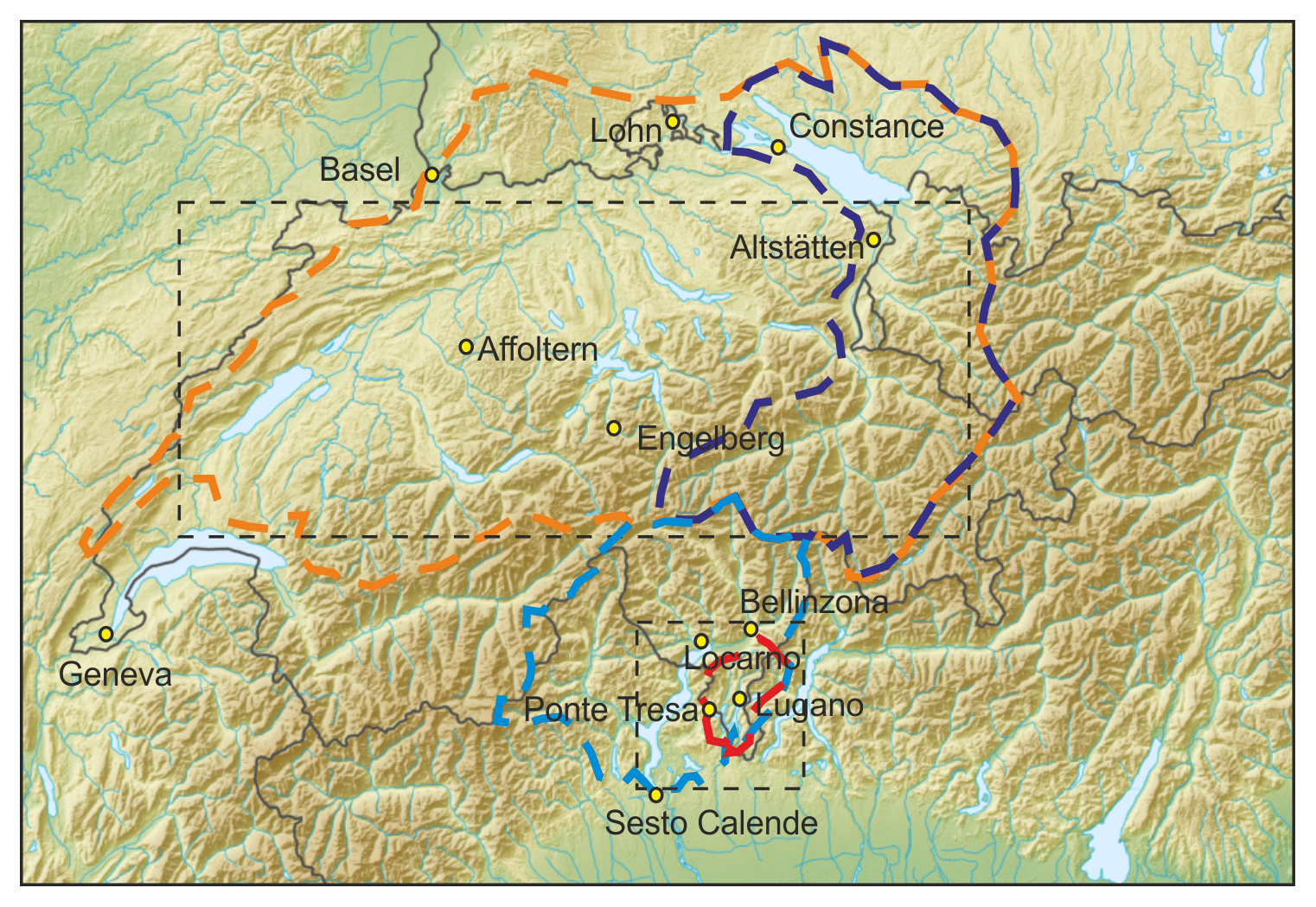
Figure 1Topographic map of the central Alps showing the catchments and locations mentioned in the text, the catchments of the Rhine in Basel (orange), Lake Constance (dark blue), Lago Maggiore (light blue) and Ponte Tresa (red). The rectangle boxes indicate the areas chosen for averaging precipitation in the HISTALP data.
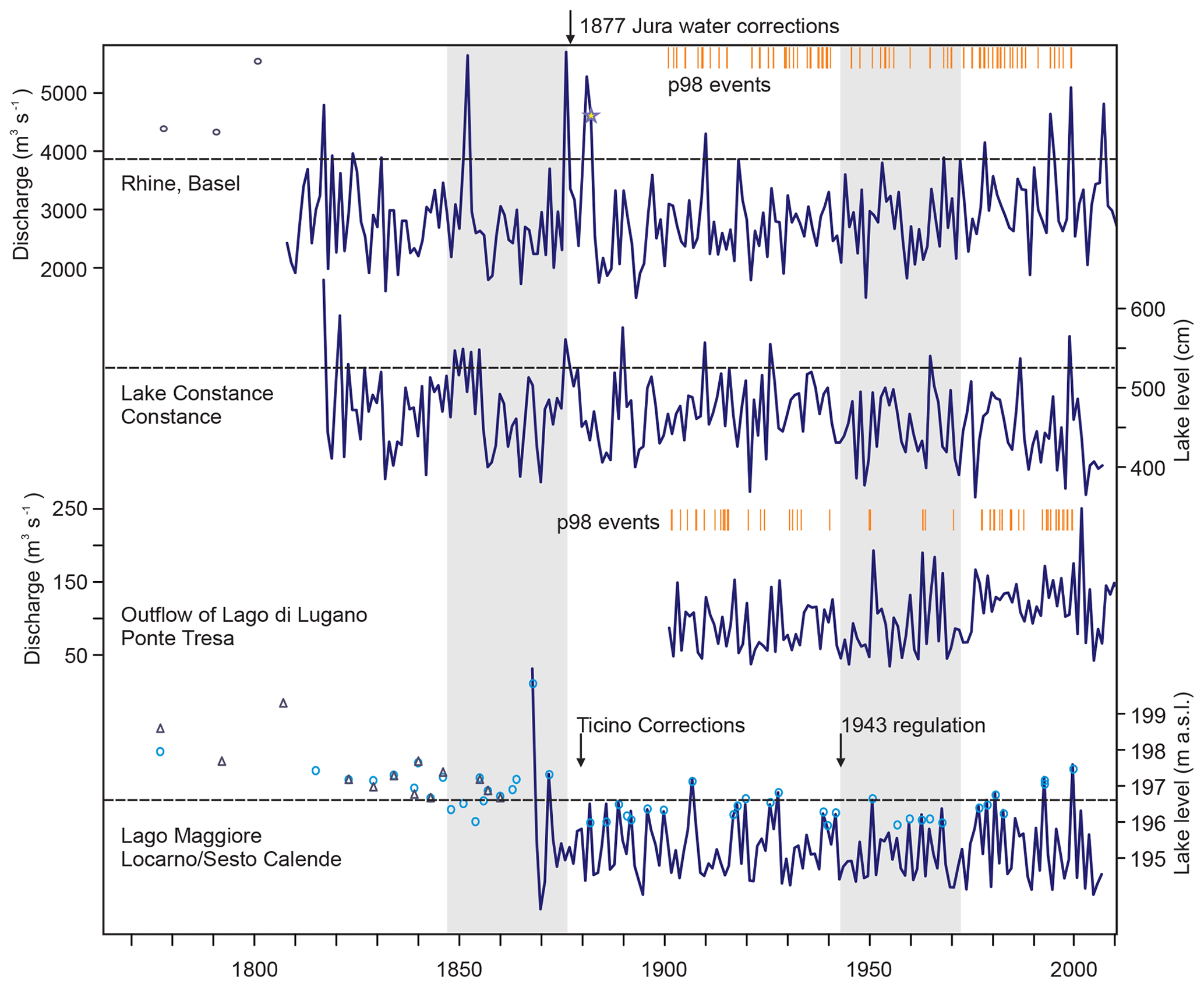
Figure 2Time series of annual maxima of discharge or lake level in four catchments. Symbols denote reconstructed floods based on historical sources (circles for Rhine, Basel, from Wetter et al., 2011; triangles for Lago Maggiore, Locarno, from Stucki and Luterbacher, 2010; light blue circles for Lago Maggiore refer to floods at Sesto Calende according to Di Bella, 2005, from reconstruction prior to 1829 and measurements afterwards, adjusted to Locarno by adding the average difference between the two during floods after 1868, i.e., 0.49 m). Arrows indicate major river corrections. Orange bars indicate the peak-over-threshold events in the 1901–2000 period that were used to calibrate the FPI. Gray shading denotes the flood-rich period (1847–1876) and flood-poor period (1943–1972). Dashed lines indicate the 95th percentile from 1901 to 2000. The star marks the Christmas flood of 1882.
Some of the series have potential inhomogeneities. Major corrections in the catchments or lakes were carried out in 1877 (Jura water correction, affecting the Aare and thus the Rhine), between 1888 and 1912 (Ticino in the Magadino plain), and 1943 (regulation of the level of Lago Maggiore). Lake Constance was and still is unregulated, but Jöhnk et al. (2004) argue that the level decreased by 15 cm between 1940 and 1999 due to upstream reservoirs. Based on model simulations, Wetter et al. (2011) estimate that the Jura water correction led to a reduction in peak discharges in Basel by 500 to 630 m3 s−1. A further possible inhomogeneity concerns the level of Lago Maggiore. The flood of 1868 reportedly led to erosion at the outflow, lowering the peak lake levels after the event. We will address these issues in Sect. 3. Note that in terms of underlying processes, lake floods slightly differ from river floods. They depend on the antecedent lake level, which carries a longer memory with it.
2.2 Precipitation data
Unfortunately, hardly any daily precipitation series covers the entire, approximately 200-year period considered here. The only long series in Switzerland is from Geneva (Füllemann et al., 2011), with daily precipitation data reaching back to 1796. Note that this series was not homogenized prior to 1864, and that it might not be representative of the northern side of the Alps. Much more daily records exist from Switzerland from 1864 onward, the start of the Swiss network. We use data for Lugano (Ponte Tresa catchment), as well as from a number of other stations (Affoltern, Basel, Altstätten, Bellinzona, Lohn, Engelberg; see Fig. 1). Monthly precipitation was taken from the gridded HISTALP (Historical Instrumental Climatological Surface Time Series of the Greater Alpine Region) data set (Hiebl et al., 2009).
Earlier studies (e.g., Glaser et al., 2010; Stucki et al., 2012) indicate that in the region of interest, most floods occur in the warm season (hereafter May to October). The only notable exception is the Christmas flood of 1882 (marked by a star in Fig. 2). In this paper, we therefore show the results only for the warm season. From both daily precipitation series we calculate the maximum precipitation amount over 3 d per warm season, denoted Rx3day. From the gridded HISTALP data set we calculated warm-season precipitation averages for two regions (Fig. 1): a region north (46.5–47.5∘ N, 6.5–10∘ E) and a region south (45.75–46.25∘ N, 8.5–9.25∘ E) of the Alpine divide.
2.3 Weather type reconstruction
In order to address flood-inducing weather patterns, we use the daily weather type reconstruction for Switzerland by Schwander et al. (2017), which reaches as far back as 1763. The weather types used in this paper are an extension of the CAP9 weather types of MeteoSwiss (Weusthoff, 2011) into the past, using station data and classifying each day according to its Mahalanobis distance from the centroids of the weather types in the calibration period. However, as two of the types were not well discernible from two other types, the respective types were merged such that only seven types remain (CAP7; see Schwander et al., 2017). This assures a good quality of the reconstruction. After 1810, the probability of each day being attributed to the right class is higher than 80 %; after 1860 it is higher than 85 % (see Schwander et al., 2017). Figure 3 shows the averages of sea-level pressure per CAP7 weather type.
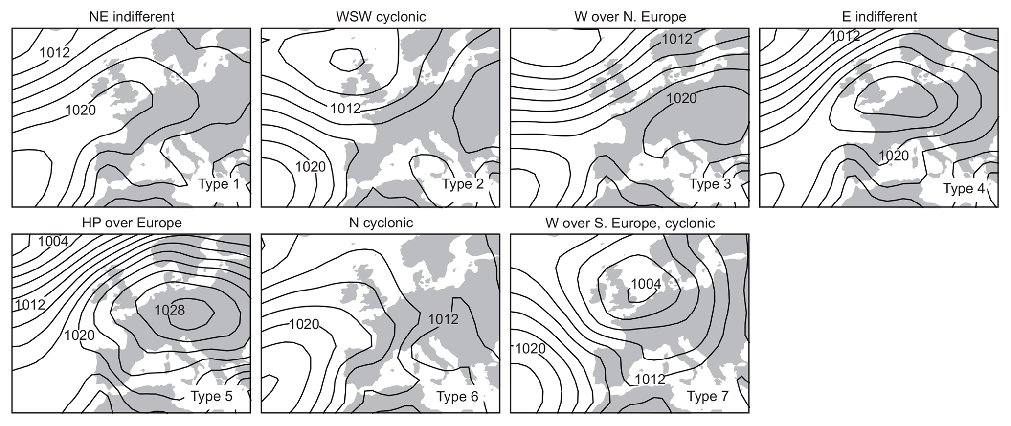
Figure 3Sea-level pressure averaged for each of the 7 weather types in CAP7 over the warm season (May–October) for the period 1958–1998 based on 20CRv2c.
2.4 Reanalyses
To corroborate our results, we also consulted the Twentieth Century Reanalysis, version 2c (20CRv2c; Compo et al., 2011). Specifically, we used daily data of precipitation, precipitable water (PWAT), and u wind at 850 hPa for the grid point 48∘ N, 6∘ E, representing the Basel catchment. From these data we calculated Rx3d as well as a u850 hPa*PWAT as a measure of moisture transport from the west towards the Alps. This is important as so-called “atmospheric rivers” are important precursors to Alpine flood events (Froidevaux and Martius, 2016). We also calculated CAP7 weather types from 20CRv2c as described in Rohrer et al. (2018). In brief, we attributed each day to the closest circulation type centroid according to its Euclidian distance. Centroids were defined in 1957–2010 based on the MeteoSwiss classification (Weusthoff, 2011). Note that all calculations were performed for each of the 56 members of 20CRv2c individually.
2.5 Climate model simulations and reconstructions
For the analysis of atmospheric circulation during the 19th and 20th century, we use the reconstruction EKF400 (Reconstruction by Ensemble Kalman Fitting over 400 years; Franke et al., 2017a). This global, three-dimensional reconstruction is based on an off-line data assimilation approach of early instrumental, documentary, and proxy data into an ensemble of climate model simulations. It provides an ensemble of 30 monthly reconstructions back to 1600. Here we use the ensemble mean and analyze geopotential height (GPH) and vertical velocity at 500 hPa, wind at 850 hPa, and precipitation.
Finally, we compare the observations-based results with a large ensemble of climate model simulations. We use a 30-member ensemble of atmospheric simulations performed with ECHAM5.4 (T63) termed CCC400 (Chemical Climate Change over 400 years), which is the set of simulations that also underlies EKF400. The simulations cover the period 1600 to 2005 and are described in Bhend et al. (2012). Their most important boundary conditions are sea-surface temperature (SST) data by Mann et al. (2009). From these SSTs we also calculated indices of the Atlantic Multidecadal Oscillation (AMO) and the Pacific Decadal Oscillation (PDO) following the definitions by Trenberth and Shea (2006) and Mantua et al. (1997), respectively (see Brönnimann, 2015, for extensive comparisons of these indices and CCC400 results). Note that in these simulations, the long-term changes in land-surface properties were misspecified. We therefore performed an additional simulation with corrected land surface to assess the impacts (Rohrer et al., 2018). While no impacts were found in heavy precipitation and weather types, warm-season average precipitation showed too strong a drying trend, which we adjusted to match that of the corrected simulation. In any case, the discrepancy concerns the long-term change and not decadal-to-multi-decadal variability.
Similarly as for 20CRv2c, we use daily precipitation representative of the Aare catchment (47.5∘ N, 7.4∘ E; see Brönnimann et al., 2018) and the CAP7 weather types from CCC400. The CAP7 weather types were evaluated by Rohrer et al. (2018): although the model shows a zonal bias (too frequent westerly types), the decadal variability of weather type frequencies within the simulations may give some indications as to a possible contribution due to SST anomalies or external forcings.
2.6 Construction of a flood probability index
From the weather types described above, we construct a flood probability index (FPI) for each river catchment following the basic methodology of Quinn and Wilby (2013). The FPI weighs the frequency of weather types according to their flood proneness. To determine the weights, we used daily discharge data during the period 1901–2009 for Basel and Ponte Tresa. Flood events were defined using a peak-over-threshold approach. The 98th percentile of warm-season days was taken as a threshold, and a declustering was applied by combining events with a maximum distance of 3 d. Compositing the events around the day of maximum discharge showed enhanced discharge already several days prior to the event. Therefore, we also considered weather types on 5 d prior to the event (Froidevaux, 2014, analyzing the role of antecedent precipitation for floods in Swiss rivers, find a somewhat shorter interval but analyzed smaller catchments). In the following we analyze the weather types during flood events and the preceding 7 d.
Figure 4a shows the frequency of weather types during all warm-season days for the period 1901–2000. The types “northeast, indifferent”, “west–southwest, cyclonic”, and “east, indifferent” make up 60 % of all days. The rarest weather type “high pressure” accounts for 5 % of all days. Panels b and c show the fraction of flood events per weather type for Basel and Ponte Tresa (dividing the fractions in the panel c series by the frequencies in panel a yields wtl in Eq. 1). Of all flood days in Basel, 60 % are either “northeast”, “indifferent”, or “north cyclonic“ types. The 2 d prior to the event are dominated (77 %) by the three “cyclonic” types, and an increase in cyclonic types is even found 5 d ahead of the flood event (65 % versus 42 % on average). For Ponte Tresa, type 7 (“westerly over southern Europe, cyclonic”) is the most flood prone, followed by “west–southwest cyclonic”. The former dominates particularly 1 to 5 d ahead of the event. On these days, type 7 is 4 times more frequent than the average on all days.
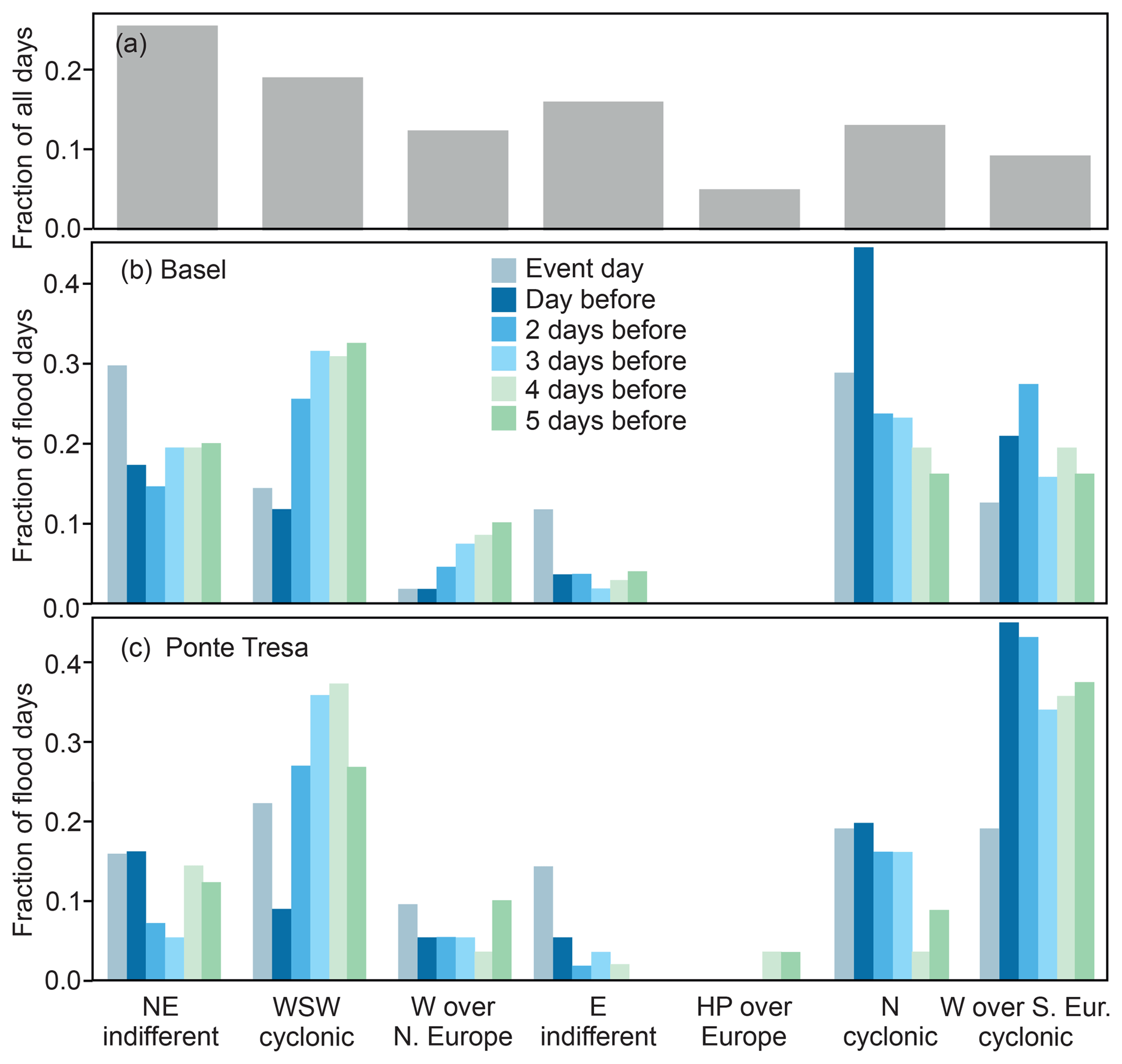
Figure 4Frequency of CAP7 weather types in the warm season (a). Fraction of flood days occurring during specific weather types for Basel (b) and Ponte Tresa (c) as well as corresponding series for days 1 to 5 prior to the discharge peak. The figure is based on data from 1901 to 2000.
A seasonal or annual flood probability index FPIy can be defined in the following way. For all event days in our calibration period 1901–2009 (and similarly for preceding days, l indicates the lag and ranges from −5 to 0), we analyzed the absolute frequency of a given weather type t (nt) relative to all event days (nl) and divided this by the absolute frequency of that weather type on all days (nt). This ratio was termed wtl:
To determine the FPI for a given year y (in our case, a warm season) we analyzed the absolute weather type frequencies in that year (warm season), nty and multiplied it with the corresponding weights wtl for a given lag l. This results in one time series for each lag l. The six series were then combined to provide the index FPIy using a weighted average with weights vl:
Based on the results of Fig. 4, the weights (vl) for days −5 to 0 were set to 1∕16, 1∕8, 3∕16, 1∕4, 1∕4, and 1∕8 (assigning equal weights or using a shorter window yields very similar results). Note that weights were recalculated for the FPI from 20CRv2c.
Quinn and Wilby (2013) used annual frequencies of the weather types to define the FPI. Here we calculated a daily index FPId, which (unlike the annual index) takes the actual sequence of weather types into account, such as during the passage of a cyclone. Equation (2) can be used for the daily index, with the same weights vl and wtl as for FPIy, but the frequency ntdl is now either 0 or 1:
The result is a daily index FPId, whose warm-season average is by definition equal to FPIy but which also allows studying other statistics. To test the daily index for the case of Basel, we studied composites of FPId, average daily precipitation from all sites north of the Alps (Affoltern, Altstätten, Basel, Engelberg, Geneva, and Lohn), moisture transport u850*PWAT from 20CRv2c, and discharge in Basel for two types of composites: (1) for peak-over-threshold flood events and (2) for peak-over-threshold events of FPId (defined in the same way, i.e., as declustered 98th percentile). As expected, flood events are related to a clearly increased FPId (Fig. 5, left). The average reaches 1.67, which means a 67 % increase in flood probability. This corresponds to the 83rd percentile of FPId. Moisture transport is increased (to its 75th percentile) 5 to 2 d prior to the flood event. Precipitation reaches its 97th percentile on days 1 and 2 prior to the event. The mean of the selected flood events corresponds to a quantile of 99.4 %. Compositing the same variables for instances with a high FPId (Fig. 5, right), we find a similarly high percentile (99.3 %) for the mean of the selected FPId events. We also find high moisture transport (79th percentile) and precipitation (89th percentile) 2 d ahead of the event. The FPId clearly captures the passage of active cyclones. Discharge in Basel is also increased but only to its 71st percentile.
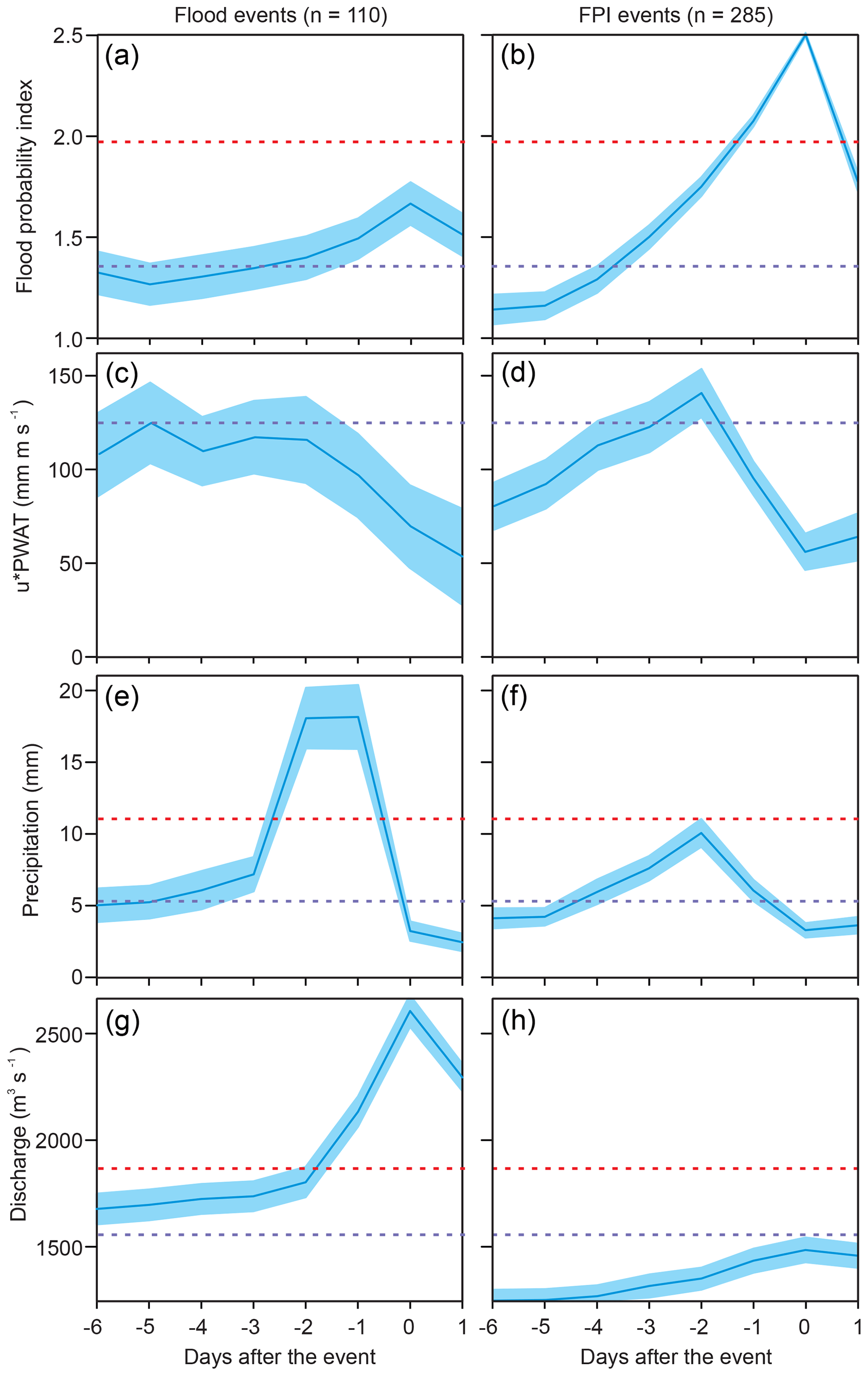
Figure 5Composites of FPId, u850 hPa*PWAT, precipitation, and discharge in Basel for (a, c, e, g) flood events in Basel and (b, d, f, h) FPId events in 1901–2000 for 6 d preceding to 1 d following event day (day 0). Shading indicates 2 standard deviations. The red and purple dashed lines indicate the 90th and 75th percentile, respectively.
Thus, the index captures flood events and also moisture transport and precipitation well, although with a high rate of “false alarms” (i.e., not all FPId events lead to floods). This can be expected for such a coarse classification. Classifications with more types were also reconstructed, but less skillfully, and hence we prefer CAP7 (Schwander et al., 2017). Another cause are the preconditions for flood events, particularly for such a large catchment as the Rhine. Discharge in Basel is on average above its 75th percentile already a week or more prior to the event, perhaps due to the passage of previous cyclones (not captured in FPId). A third cause of false alarms is the different sample size of flood events (n=110) and “FPI events“ (n=285) despite using the same threshold and declustering. This is due to the different temporal structure of the time series. Two thirds of the FPId events cannot be floods even if the match was perfect.
High percentiles of FPId are thus not suitable for studies of interannual-to-decadal variability. Flood-conducive cyclone passages occur almost every summer and hence high percentiles of FPId show little interannual variability. We use the warm-season 75th percentile to capture the upper part of the distribution as well as the 50th percentile and the mean (i.e., FPIy) to capture the central tendency
3.1 Flood frequency
To begin with, we analyzed the flood series in order to test whether the reported increased flood frequency in the mid-19th century is also found in our series (Fig. 4). The first thing we note is that floods do not occur synchronously across the considered catchments. The same is true for annual peak discharge series in general, as evidenced by low Spearman correlations. For instance, the series for the Rhine in Basel is uncorrelated with the series of Lago Maggiore and only moderately (coefficient of 0.36) with the series of Lake Constance, even though the latter comprises a large sub-catchment.
Was flood frequency higher in the mid-19th century? In fact, each series exhibits prominent peaks in the 19th century, e.g., the Rhine in Basel in 1817, 1852, 1876, 1881, and 1882 (see Stucki et al., 2012), Lake Constance in 1817 (see Rössler and Brönnimann, 2018), and Lago Maggiore in 1868 (Stucki et al., 2018). However, we also note a period of low flood frequency in Basel from the 1920s to 1970s, in agreement with a low frequency of peak-over-threshold events in Basel and Ponte Tresa. For further analyses we defined the 30-year periods with the highest and lowest flood frequencies as follows: from the annual series we defined floods as exceedances of the 95th percentile of the 1901–2000 period (dashed line). Note that even accounting for a shift of 630 m3 s−1 due to the Jura water correction would not change the selected events of the Rhine in Basel, neither would a correction for a linear 15 cm trend of Lake Constance after 1940 due to an increasing number of water reservoirs upstream (see Jöhnk et al., 2004). However, the inhomogeneity caused by the 1868 event might be substantial. We therefore considered pre-1868 data only qualitatively.
Counting annual floods in all series as well as counting the daily peak-over-threshold events for Basel and Ponte Tresa both yield the same 30-year period with the lowest flood frequency: 1943–1972. The period with highest flood frequency is only defined by counting annual floods. Not including pre-1868 Lago Maggiore data, the period 1847–1876 is the most flood-rich. This is further supported by the historical data for Lago Maggiore, which suggest additional strong flood events in that period. However, earlier 30-year periods might be equally or even more flood-rich, according to reconstructed flood events.
In the following we assess differences in a variable in each period relative to a corresponding climatology (a sample consisting of 30 years before and 30 years after the period to further reduce the effect of centennial-scale changes) as well as between the two periods with a Wilcoxon test.
3.2 Precipitation
In a second step, we analyzed warm-season mean precipitation and Rx3day for the regions north or south of the Alps (Figs. 6 and 7). In both regions, warm-season precipitation is correlated significantly (Spearman correlation of 0.45 and 0.50, respectively) with annual maximum discharge, clearly indicating that the floods under study are caused by excess precipitation. In both regions, precipitation was slightly above the 20th century mean (dashed) during most of the 19th century and below average during the flood-poor period. The difference between the flood-rich (1847–1876) and the flood-poor (1943–1972) periods is significant (p value of the Wilcoxon test: p=0.027) for the Ponte Tresa catchment. For the Basel catchment, both periods deviate significantly negatively from the corresponding neighboring decades (p=0.049 and 0.030 for the flood-rich and flood-poor period, respectively), which is unexpected for the flood-rich period. Their difference is not significant.
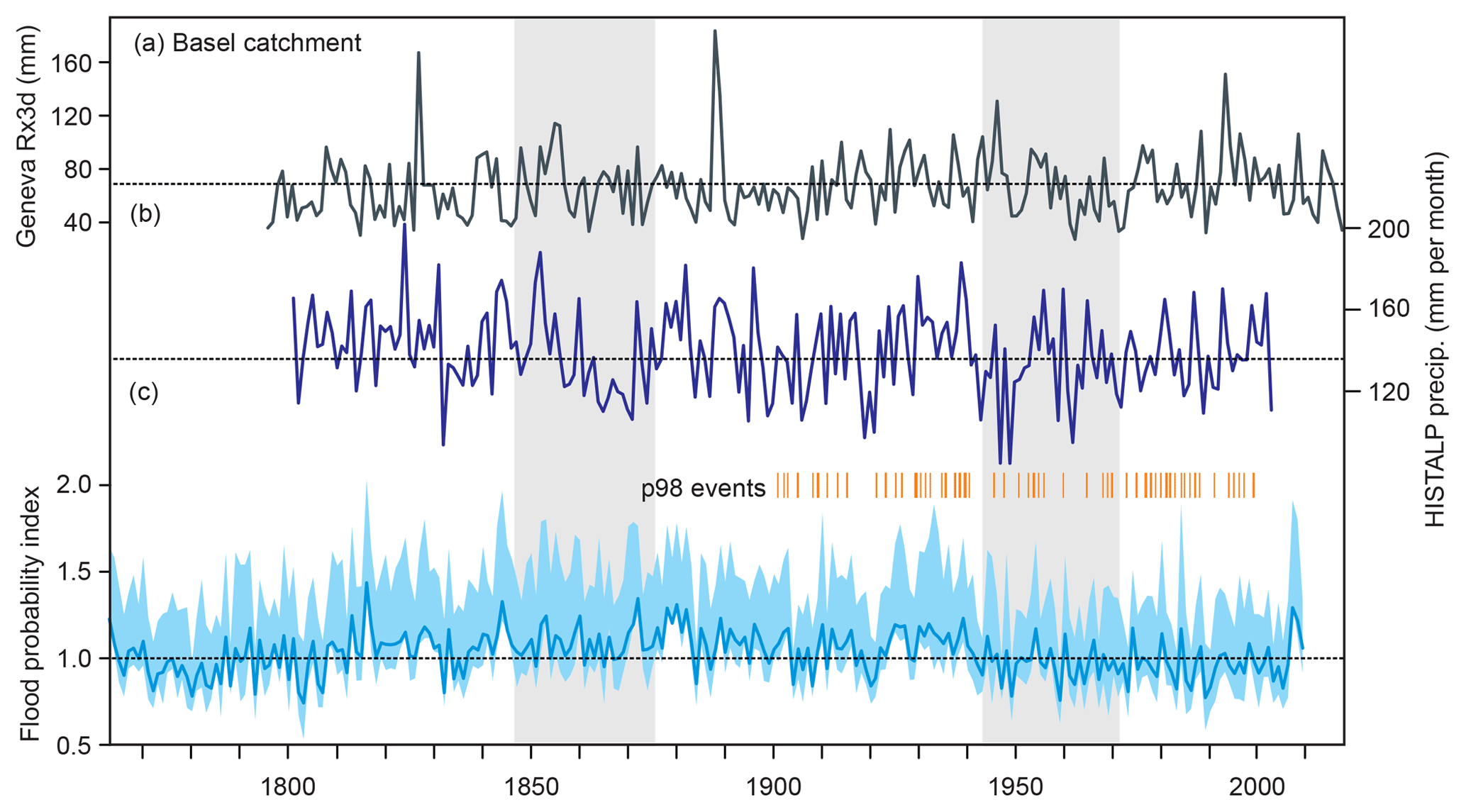
Figure 6Warm-season Rx3d from the station Geneva (a), warm-season mean precipitation in HISTALP for the Rhine catchment (b), and flood probability index for Basel (c; solid indicates the warm-season mean, and blue shading indicates the median and 75th percentile). Dashed lines indicate the 1901–2000 average. Also shown are the peak-over-threshold events (p98) of Basel discharge that were used for calibration. Gray shading denotes the flood-rich period (1847–1876) and flood-poor period (1943–1972).
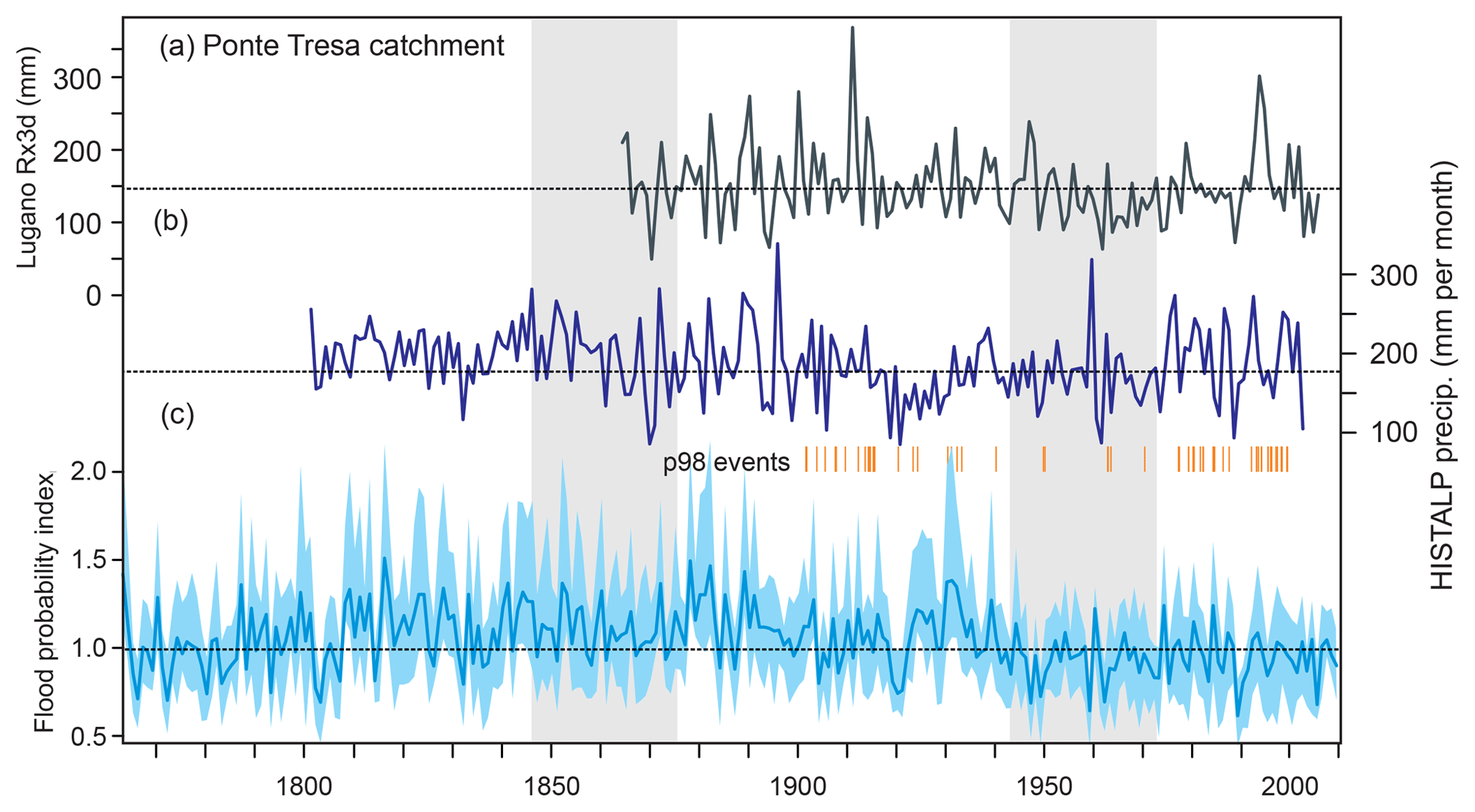
Figure 7Warm-season Rx3d from the station Lugano (a), warm-season mean precipitation in HISTALP for the Ponte Tresa catchment (b), and flood probability index for Ponte Tresa (c; solid indicates the warm-season mean, and blue shading indicates the median and 75th percentile). Dashed lines indicate the 1901–2000 average. Also shown are the peak-over-threshold events (p98) of Ponte Tresa discharge that were used for calibration. Gray shading denotes the flood-rich period (1847–1876) and flood-poor period (1943–1972).
Rx3day for Geneva and Lugano are shown exemplarily to assess the role of extreme precipitation. For Geneva, we find two pronounced extremes (1827, 1888), both of which were discussed in newspapers (anonymous, 1827) and thus are considered real. For both stations, the decreased intensity of Rx3d in the flood-poor period relative to neighboring decades is significant (p=0.026 and 0.038 for the Rhine and Ponte Tresa catchments, respectively). A similar decrease at the same time is also found for other series in Switzerland (Fig. 8 shows six long series). Calculating for each series the annual exceedance frequency of the 95th percentile (based on the 1901–2000 interval) of Rx3d and then averaging over all eight series shown in Figs. 6 to 8, we obtain a time series of the ratio of stations exceeding their 95th percentile in a given year. This series shows lower values in the 1943–1972 period than in the following 30-year period and even lower than in the late 19th century.
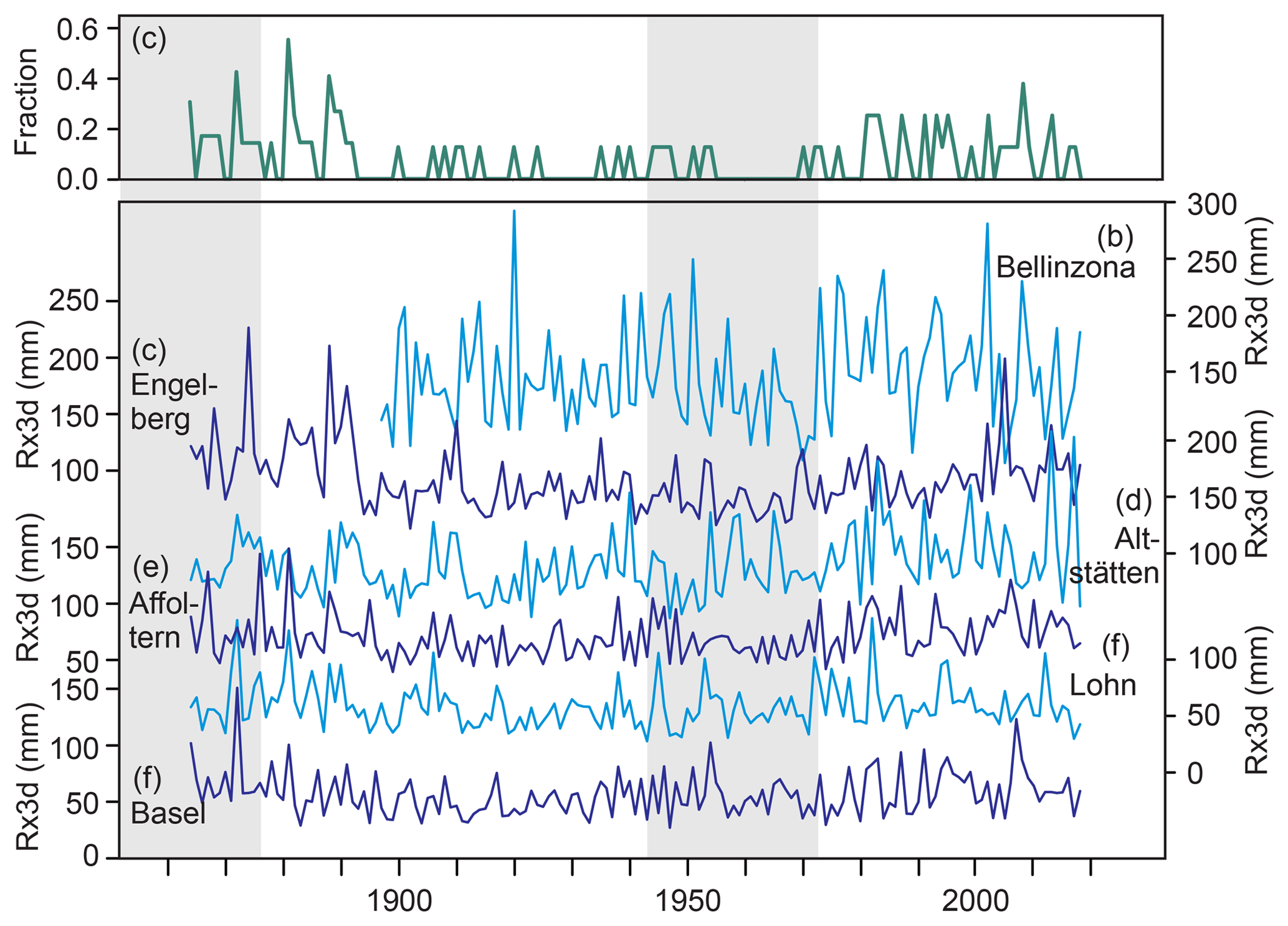
Figure 8Series of Rx3day for six further stations with long precipitation series (see Fig. 1 for locations). The top line shows the fraction of these six series plus those of Lugano and Geneva shown in Figs. 5 and 6, exceeding their 95th percentile (based on 1901–2000) in any given year. Gray shading denotes the flood-rich period (1847–1876) and flood-poor period (1943–1972).
In Sect. 3.1 we found clear changes in flood frequency. This section shows that at least the flood-poor period was related to a reduction in the precipitation amount and intensity of Rx3d events, while results for the flood-rich period are ambiguous.
3.3 Moisture transport
In addition, we consider moisture transport from the west towards the Alps, which we analyze in 20CRv2c for the Basel catchment. Similarly to Rx3d, as a diagnostic we calculate the largest 3 d average of u850 hPa*PWAT per summer season. This proxy for westerly moisture transport is shown together with Rx3d and FPIy (both also calculated from 20CRv2c) in Fig. 9. For Rx3d and FPIy we also show the observations-based series.
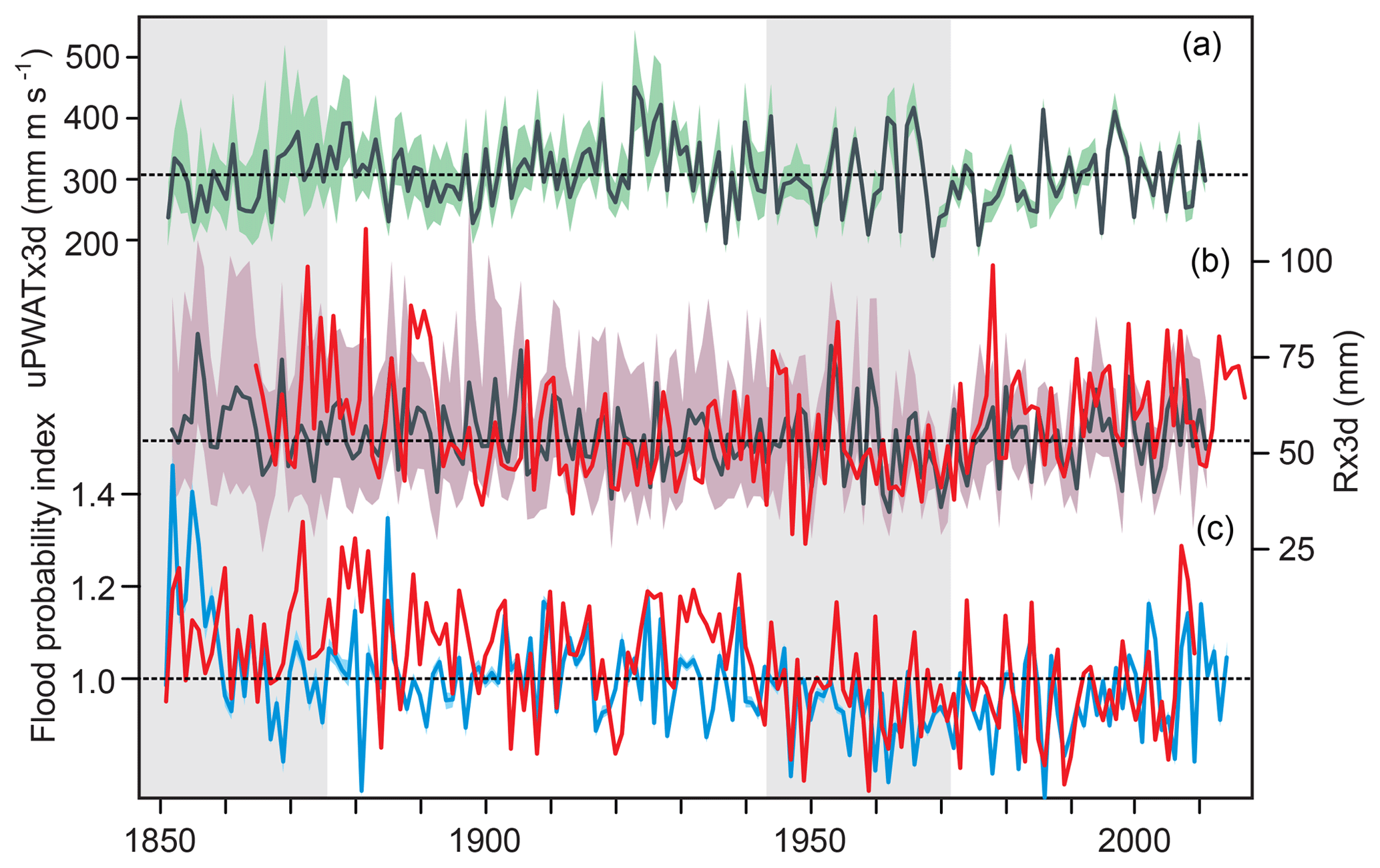
Figure 9Maximum 3 d average per warm season of (a) eastward moisture transport (u850 hPa*PWAT) and (b) precipitation, both at the grid point 48∘ N, 6∘ E in 20CRv2c. Panel (c): warm-season mean FPI index in 20CRv2c. Shading denotes the ensemble range (min and max). Red lines show the corresponding series from observations (Rx3d is calculated from the average of all stations north of the Alps). Dashed lines indicate the average value for 1901–2000 in 20CRv2c. Gray shadings denote the flood-rich (1847–1876) and flood-poor (1943–1972) periods.
Results for the flood-rich period are ambiguous, and discrepancies with the observations-based series are large in parts, as is seen in FPId in the 1850s and 1880s in Fig. 9. This may be explained by the fact that 20CRv2c is prone to errors in the early decades (see Rohrer et al., 2018). Agreement between observations and 20CRv2c increases after 1900. Specifically, moisture transport shows similar decadal variability as FPI or precipitation, with higher values prior to 1940 and lower values afterwards. Although 20CRv2c alone does not permit the interpretation of decadal changes, we note that the changes are fully consistent with those in our independent time series.
3.4 Weather and large-scale flow
In the next step, we analyze the link of flood events to atmospheric circulation and its multi-decadal changes by means of the FPId statistics (see Sect. 2.5). The temporal development for Basel (Fig. 6c) and Ponte Tresa (Fig. 7c) is similar for all indicators (mean, median, or 75th percentile), and the Spearman correlations of the Basel FPId series with the annual maximum discharge at Basel are statistically significant (p=0.005 to 0.014). This shows that the FPI is a good predictor for flood variability.
For both catchments, the indices reveal clear multi-decadal variability. Indices are generally positive from the 1810s to 1900s (with a secondary maximum in the 1920s and 1930s) and negative from the 1940s to around the 2000s. Both periods are longer than those selected in our study. The differences in the FPId between our flood-rich and flood-poor period is significant in both catchments for all three indices (max p value is 0.0023). The flood-rich period does not differ significantly from the neighboring decades (which also show high values of the FPI) in any of the indices, whereas the flood-poor period shows lower values than the neighboring decades (p=0.047 and 0.067 for Basel and Ponte Tresa, respectively). From these analyses we can conclude that the change in precipitation amount and intensity found in the previous section was related to the FPI. The flood-rich and flood-poor periods clearly differ with respect to occurrence of weather types, i.e., large-scale atmospheric flow.
Floods are extreme and thus rare events, but the causes of changes in extremes do not need to be rare. Changes in extremes may be the expression of a shift in the underlying distribution. For instance, the correlations of the 75th and 90th percentile of FPId with the mean are 0.92 and 0.77 for the Basel catchment and 0.95 and 0.91 for the Ponte Tresa catchment. Additionally, for the case of floods, Fig. 5 shows that preconditions (and thus the previous cyclone) matter. We therefore analyze to what extent the change in weather types is mirrored in the multi-decadal atmospheric circulation statistics.
We analyzed the two periods in global climate reconstructions (EKF400), each relative to its climatology as well as the difference between the two (Fig. 10). The anomalies for the flood-rich period show clear negative GPH anomalies over western Europe and strengthened flow from the northwest. The extension of the Azores onto the European continent weakened. This pattern becomes a lot stronger and clearer when contrasting the two periods (flood-rich minus food-poor). The anomalies for the flood-poor period show strengthened high-pressure influence over central Europe and descent and dryness with anomalous flow from the northeast.
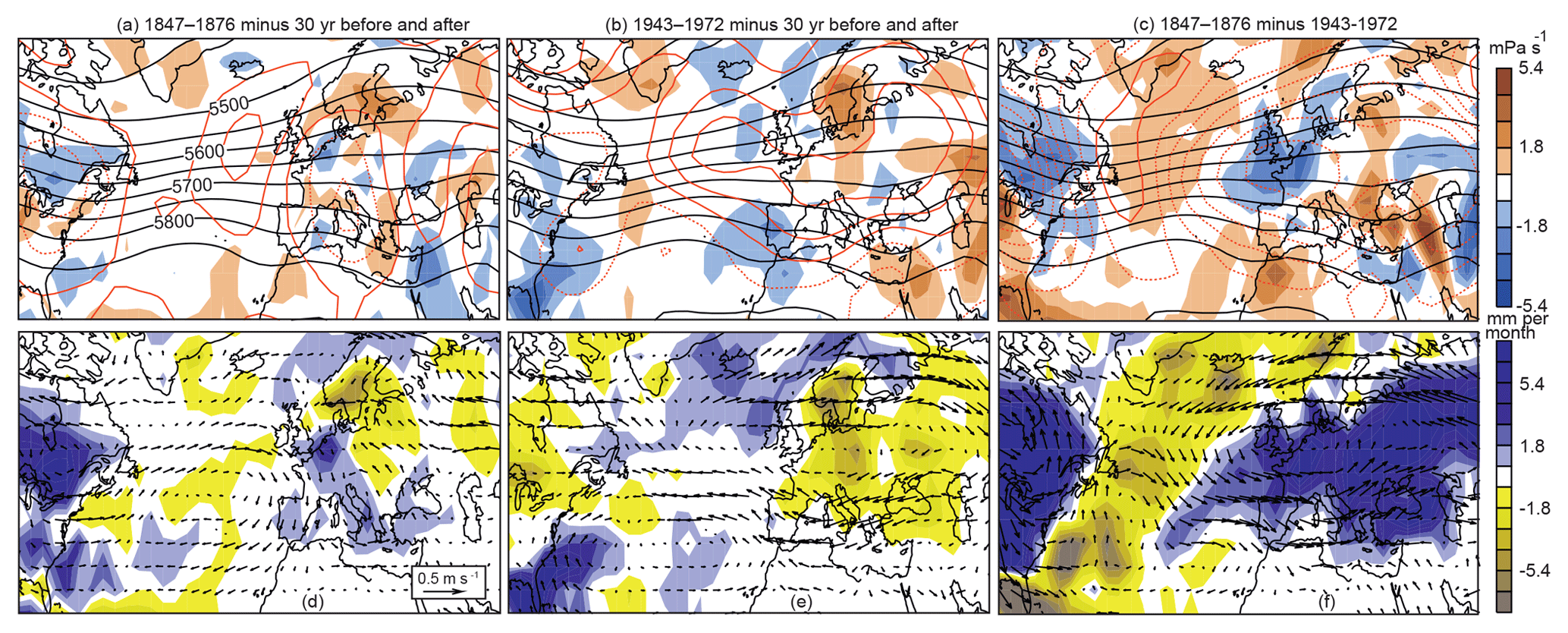
Figure 10Anomalies of (a–c) 500 hPa GPH (red contours, 2 gpm – geopotential meters – spacing symmetric around 0; negative contours are dashed; black lines indicate the reference period average) and vertical velocity (colors; lifting is blue) and (d–f) 850 hPa wind and precipitation. Shown are anomalies for the 1847–1876 period (a, c) and the 1943–1972 period (b, d) with respect to the 30 years before and after as well as (c, f) the difference between the two periods.
In all, the large-scale analysis confirms the results from the FPI: it shows clearly that the shift in weather types was an expression of multi-decadal variability of atmospheric circulation over the full North Atlantic–European sector, consisting of a more zonal and southward-shifted circulation.
3.5 Climate model simulations
We have seen that the decadal-to-multi-decadal changes in flood frequency can be related to changes in weather types, which are part of large-scale flow anomalies. In the fourth step, we analyzed whether this can in turn be attributed to influences such as sea-surface temperature variability modes as depicted by atmospheric model simulations (CCC400) or whether the decadal-to-multi-decadal changes are due to random, possibly atmospheric variability. Concretely, we analyzed warm-season mean precipitation and Rx3d for a grid point north of the Alps and calculated FPId and its statistics for each member. We then averaged the results across all 30 CCC400 members (one corrupt member was excluded for FPIy). This is meaningful because changes in the ensemble mean reflect a common signal which must be due to the common boundary conditions of the simulation. Figure 11 shows the series in a smoothed form (31-year moving average) for visualization.
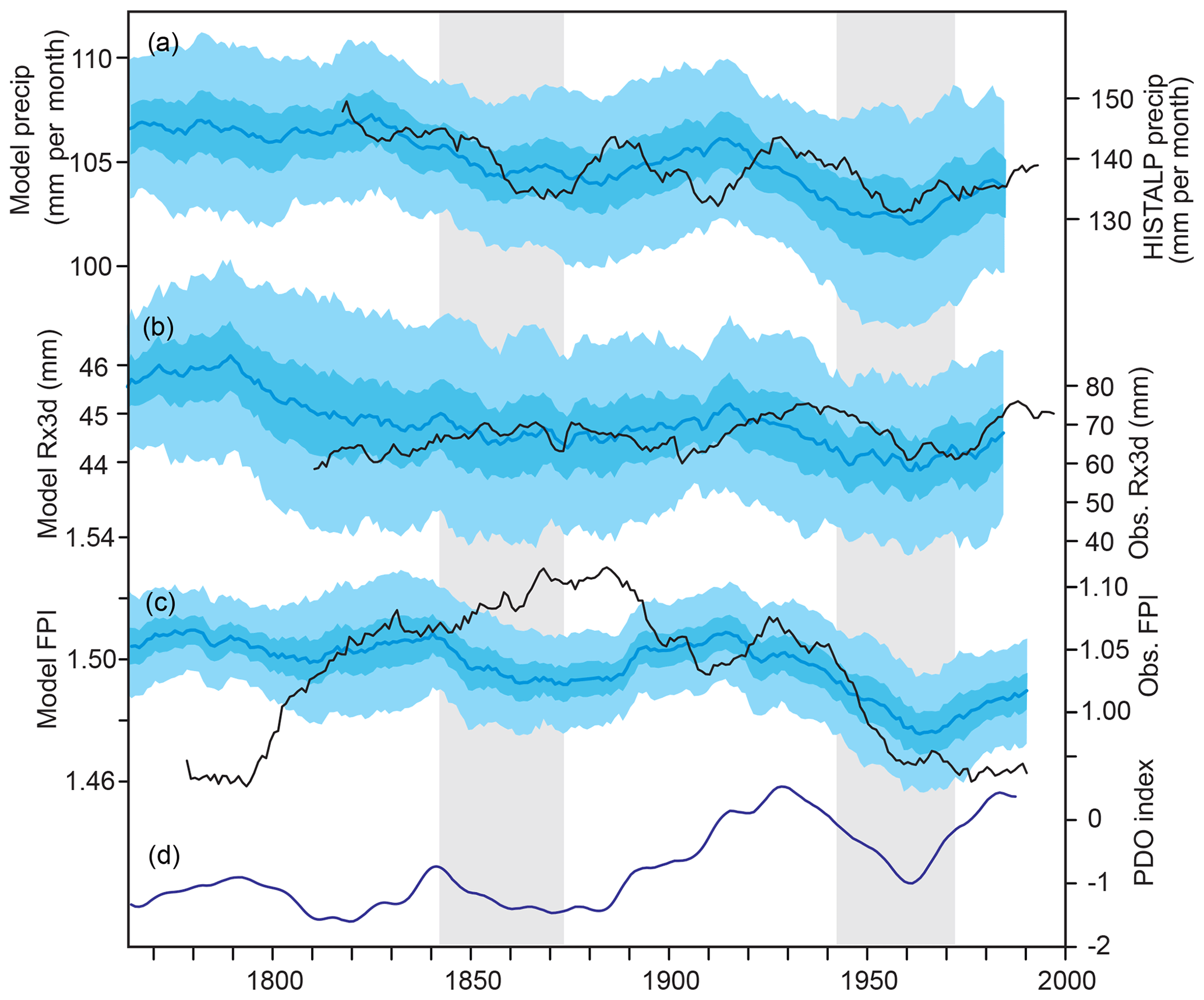
Figure 11CCC400 (left scales) warm-season average precipitation (a; note that this series was detrended based on the corrected member), Rx3day in the warm season at the grid point north of the Alps (b), and flood probability index based on weather types in CCC400 (c). Panel (d) shows the PDO index in the model simulations. The solid blue lines show the ensemble mean of the series smoothed with a 31-year moving average. Light and dark shadings indicate the ensemble standard deviation and the 95 % confidence interval of the ensemble mean, respectively. Black lines (right scales) show the corresponding observation-based series. Note the different scales. Gray shadings denote the flood-rich (1847–1876) and flood-poor (1943–1972) periods.
Indeed, we note that the agreement between modeled and observation-based FPI is not good in the 19th century; the broad 19th century peak in the observation-based FPI is missing in the model. In addition, the analysis reveals downward trends in mean precipitation (although the series is trend-corrected) as well as in Rx3d. Quantitatively, the trend in mean precipitation amounts to −1.88 % per century, which is rather small (much smaller than in the observations). Due to this trend it is not surprising that significant differences in seasonal mean precipitation appear between the two periods, which may be unrelated to decadal-to-multi-decadal variability but rather to multi-centennial trends. Differences between the averages of the flood-rich and the flood-poor periods across the ensemble are not significant for Rx3d and around the significance limit for FPIy (Wilcoxon test: p=0.043).
In the model, the flood-rich period is not significantly different from neighboring decades in any of the measures, but the flood-poor period appears as a potentially flood-poor period in seasonal mean precipitation and FPIy (Wilcoxon test: p=0.013 and p=0.004, respectively). Only model boundary conditions can explain this, and the arguably dominant contribution is from SSTs. Among the well-known SST variability modes, it is in fact the PDO index that explains the FPIy most successfully. However, the Spearman correlation remains low and not significant in view of the low number of degrees of freedom, even after detrending.
We infer from these analyses that our climate model simulations do not reproduce the flood-rich period, but the flood-poor period appears as a feature.
While tracking the flood-frequency signal, we have found a number of links and dependencies; these are discussed in the following. For instance, previous studies found an increased flood frequency in Switzerland in the 19th century (Pfister, 1984, 1999, 2009; Stucki and Luterbacher, 2010; Schmocker-Fakel and Naef, 2010a, b; Wetter et al., 2011) as well as a decrease in the mid-20th century, sometimes referred to as the “disaster gap“ (Pfister, 2009; Wetter et al., 2011). The series used in this paper confirm the general tendency. Schmocker-Fackel and Naef (2010a, b) identify 1820-1940 as a flood-rich period, while we use much a shorter period. However, our FPI is consistent with a longer flood-rich period around 1820–1940; i.e., the difference between 1820–1940 and 1943–1972 is also highly significant (p < 0.00001).
Rx3day series from Geneva and Lugano together with series from a larger number of Swiss stations confirm a multi-decadal period around the 1960s with reduced intensity of Rx3d. The change in the frequency of floods, which are rare events, is related to a change in mean climate. For instance, warm-season mean precipitation shows changes that are concurrent with those of flood frequency, with significant correlations. We also find consistent changes for high percentiles of the FPI and its mean.
Schmocker-Fackel and Naef (2010a) analyzed the relation between floods and weather types for the period after 1945 and manual assignments based on weather reports before that year. Here we can make use of a new, daily 250-year weather type reconstruction. As in Schmocker-Fackel and Naef (2010a), we find that events south of the Alps and those north of the Alps are related to slightly different weather type characteristics, although indices for both regions are highly correlated on all timescales. Our FPI shows clear multi-decadal variability, with high values during most of the 19th century and a secondary peak in the 1920s and 1930s, and lower than average values in the post-war period. After around 1980, the FPI returned to average values. The FPI reflects passing cyclones, but it also captures episodes of strong moisture transport, and in fact annual 3 d maxima of moisture transport in 20CRv2c show similar multi-decadal variability.
In agreement with Schmocker-Fackel and Naef (2010a, b), we find no imprint on the classical North Atlantic Oscillation (NAO) pattern and also no clear weakening of the Azores high during the flood-rich period. However, we find that the extension of the Azores high onto the European continent weakened, and we find clear negative GPH anomalies over western Europe, strengthened northwesterly advection, and large-scale ascent. This indicates a more zonal, southward-shifted circulation over the North Atlantic–European sector during the flood-rich period (Brönnimann et al., 2019). Opposite anomalies, i.e., positive GPH anomalies and descent, are found for the flood-poor period, which was in fact associated with heat waves and strong droughts in central Europe. Brugnara and Maugeri (2019) find a regime shift in total precipitation and wet-day frequency for a southern region of the Alps and for a period after the 1940s which coincides with the flood-poor period.
The flood-poor period might carry imprints of oceanic influences. Sutton and Hodson (2005) related summer climate anomalies on both sides of the Atlantic in the wider 1931–1960 period to changes in the AMO. We do not find a significant correlation between our flood and precipitation indicators and the AMO; a possible relation to the PDO index is possible but not confirmed. The flood-poor period partly overlaps with a period of poleward displacement of the northern tropical belt, which is understood to be caused by sea-surface temperature anomalies and is reproduced in climate models (Brönnimann et al., 2015). Our EKF400 analysis is thus consistent with the results of the latter study.
Flood frequency in central Europe exhibits multi-decadal changes, which has been demonstrated based on historical records. The causes of the increased flood frequency in Switzerland in the 19th century as well as for the decreased flood frequency around the mid-20th century are long-standing issues. In this study we have tracked these changes from flood records through precipitation records, weather type statistics and large-scale circulation reconstructions all the way to oceanic influences as expressed in atmospheric model simulations. The change in flood frequency is arguably the expression of changes in mean climate. We attribute the changes in flood frequency to changes in mean precipitation and in the intensity of Rx3d. In turn, these are related to a change in cyclonic weather types over central Europe. These changes indicate a shift in large-scale atmospheric circulation, with a more zonal, southward-shifted circulation during the flood-rich period relative to the flood-poor period. Precipitation and circulation changes are only to a small part reproduced in climate model simulations driven by observed sea-surface temperatures, which points to random atmospheric variability as an important and complementary cause.
The analyses show that decadal variability in flood frequency occurred in the past; and it is likely to continue into the future. Better understanding its relation to weather regimes, large-scale circulation, and possibly sea-surface temperature may help to better assess seasonal forecasts and projections. Finally, the study also shows that the Quinn and Wilby (2013) methodology also works for flood risk in Switzerland.
Daily weather types from 1763 to 2007 and the FPI indices calculated in this paper are given in the Supplement. EKF400 and CCC400 data can be downloaded from the World Data Center for Climate at the Deutsches Klimarechenzentrum (DKRZ) in Hamburg, Germany (Data Citation 1; http://dx.doi.org/10.1594/WDCC/EKF400_v1, last access: 26 July 2019) (Franke et al., 2017b). Discharge data are available from the Swiss Federal Office for the Environment (FOEN), and the precipitation data are available from the Federal Office of Meteorology and Climatology MeteoSwiss. The 20CRv2c data can be downloaded from https://www.esrl.noaa.gov/psd/data/20thC_Rean/ (last access: 10 January 2019) (Compo et al., 2015).
The supplement related to this article is available online at: https://doi.org/10.5194/cp-15-1395-2019-supplement.
SB and LF designed the study and performed the analyses. MR and JF processed the CCC400 and 20CR data, and JF assisted in the analysis of EKF400. MS provided the weather type reconstruction, and PS and LF compiled and processed the discharge and meteorological data. MS and PS assisted in the interpretation. All authors contributed to writing the paper.
The authors declare that they have no conflict of interest.
This work was supported by Swiss National Science Foundation projects RE-USE (162668), EXTRA-LARGE (143219), and CHIMES (169676), by the European Commission (ERC grant PALAEO-RA, 787574), and by the Oeschger Centre for Climate Change Research. Simulations were performed at the Swiss National Supercomputing Centre CSCS.
This research has been supported by the Swiss National Science Foundation (grant nos. 162668, 143219, and 169676), the H2020 European Research Council (grant PALAEO-RA (787574)), the Oeschger Centre for Climate Change Research, University of Bern, and the Swiss Supercomputer Center CSCS (grant CCC400).
This paper was edited by Hugues Goosse and reviewed by two anonymous referees.
Anonymous: Sur un pluie extraordinaire tombée le 20 Mai 1827, dans la vallée du Léman, Bibliothèque universelle, 35, P. 84, 1827.
Bhend, J., Franke, J., Folini, D., Wild, M., and Brönnimann, S.: An ensemble-based approach to climate reconstructions, Clim. Past, 8, 963–976, https://doi.org/10.5194/cp-8-963-2012, 2012.
Bichet, A., Folini, D., Wild, M., and Schär, C.: Enhanced Central European summer precipitation in the late 19th century: a link to the Tropics, Q. J. Roy. Meteorol. Soc., 140, 111–123, 2014.
Blöschl, G., Hall, J., Parajka, J., Perdigão, R. A. P., Merz, B., Arheimer, B., Aronica, G. T., Bilibashi, A., Bonacci, O., Borga, M., Čanjevac, I., Castellarin, A., Chirico, G. B., Claps, P., Fiala, K., Frolova, N., Gorbachova, L., Gül, A., Hannaford, J., Harrigan, S., Kireeva, M., Kiss, A., Kjeldsen, T. R., Kohnová, S., Koskela, J. J., Ledvinka, O., Macdonald, N., Mavrova-Guirguinova, M., Mediero, L., Merz, R., Molnar, P., Montanari, A., Murphy, C., Osuch, M., Ovcharuk, V., Radevski, I., Rogger, M., Salinas, J. L., Sauquet, E., Šraj, M., Szolgay, J., Viglione, A., Volpi, E., Wilson, D., Zaimi, K., and Živković, N.: Changing climate shifts timing of European floods, Science, 357, 588–590, 2017.
Brönnimann, S.: Climatic changes since 1700, Adv. Glob. Change Res., 55, 360 pp., https://doi.org/10.1007/978-3-319-19042-6, 2015.
Brönnimann, S., Fischer, A. M., Rozanov, E., Poli, P., Compo, G. P., and Sardeshmukh, P. D.: Southward shift of the Northern tropical belt from 1945 to 1980, Nat. Geosc., 8, 969–974, 2015.
Brönnimann, S., Rajczak, J., Fischer, E. M., Raible, C. C., Rohrer, M., and Schär, C.: Changing seasonality of moderate and extreme precipitation events in the Alps, Nat. Hazards Earth Syst. Sci., 18, 2047–2056, https://doi.org/10.5194/nhess-18-2047-2018, 2018.
Brönnimann, S., Franke, J., Nussbaumer, S. U., Zumbühl, H. J., Steiner, D., Trachsel, M., Hegerl, G. C., Schurer, A., Worni, M., Malik, A., Flückiger, J., and Raible, C. C.: Last phase of the Little Ice Age forced by volcanic eruptions, Nat. Geosci., 1752–0908, published online, https://doi.org/10.1038/s41561-019-0402-y, 2019.
Brückner, E.: Klimaschwankungen seit 1700 nebst Bemerkungen über die Klimaschwankungen der Diluvialzeit, E. D. Hölzel, Wien and Olmütz, 1890.
Brugnara, Y. and Maugeri, M.: Daily precipitation variability in the southern Alps since the late 19th century, Int. J. Climatol., 39, 3492–3504, https://doi.org/10.1002/joc.6034, 2019.
Compo, G. P., Whitaker, J. S., Sardeshmukh, P. D., Matsui, N., Allan, R. J., Yin, X., Gleason, B. E., Vose, R. S., Rutledge, G., Bessemoulin, P., Brönnimann, S., Brunet, M., Crouthamel, R. I., Grant, A. N., Groisman, P. Y., Jones, P. D., Kruk, M. C., Kruger, A. C., Marshall, G. J., Maugeri, M., Mok, H. Y., Nordli, O., Ross, T. F., Trigo, R. M., Wang, X. L., Woodruff, S. D., and Worley, S. J.: The Twentieth Century Reanalysis Project, Q. J. Roy. Meteorol. Soc., 137, 1–28, https://doi.org/10.1002/qj.776, 2011.
Compo, G. P., Whitaker, J. S., Sardeshmukh, P. D., Matsui, N., Allan, R. J., Yin, X., Gleason, B. E., Vose, R. S., Rutledge, G., Bessemoulin, P., Brönnimann, S., Brunet, M., Crouthamel, R. I., Grant, A. N., Groisman, P. Y., Jones, P. D., Kruk, M. C., Kruger, A. C., Marshall, G. J., Maugeri, M., Mok, H. Y., Nordli, O., Ross, T. F., Trigo, R. M., Wang, X. L., Woodruff, S. D., and Worley, S. J.: NOAA/CIRES Twentieth Century Global Reanalysis Version 2, Research Data Archive at the National Center for Atmospheric Research, Computational and Information Systems Laboratory, available at: https://doi.org/10.5065/D6N877TW (last access: 10 January 2019), 2015.
Di Bella, G.: Le Piene del Ticino a Sesto Calende, Cocquio Trevisago, available at: http://www.prosestocalende.it/ (last access: 21 January 2019), 2005.
EEA: Economic losses from climate-related extremes, Copenhagen, Denmark, 17 pp., 2018.
Fischer, E. M. and Knutti, R.: Observed heavy precipitation increase confirms theory and early models, Nat. Clim. Change, 6, 986–991, 2016.
Franke, J., Brönnimann, S., Bhend, J., and Brugnara, Y.: A monthly global paleo-reanalysis of the atmosphere from 1600 to 2005 for studying past climatic variations, Sci. Data, 4, 170076, https://doi.org/10.1038/sdata.2017.76, 2017a.
Franke, J., Brönnimann, S., Bhend, J., and Brugnara, Y.: Ensemble Kalman Fitting Paleo-Reanalysis Version 1 (EKF400_v1), World Data Center for Climate (WDCC) at DKRZ, https://doi.org/10.1594/WDCC/EKF400_v1 (last access: 26 July 2019), 2017b.
Froidevaux, P.: Meteorological characterisation of floods in Switzerland, PhD Thesis, University of Bern, Bern, Switzerland, 2014.
Froidevaux, P. and Martius, O.: Exceptional integrated vapour transport toward orography: an important precursor to severe floods in Switzerland, Q. J. R. Meteorol. Soc., 142, 1997–2012, 2016
Füllemann, C., Begert, M., Croci-Maspoli, M., and Brönnimann, S.: Digitalisieren und Homogenisieren von historischen Klimadaten des Swiss NBCN – Resultate aus DigiHom, Arbeitsberichte der MeteoSchweiz, 236, 48 pp., 2011.
Glaser, R., Riemann, D., Schönbein, J., Barriendos, M., Brazdil, R., Bertoli, C., Camuffo, D., Deutsch, M., Dobrovolny, P., van Engelen, A., Enzi, S., Halickova, C., König, S., König, O., Limanowka, D., Mackova, J., Sghedoni, M., Martin, B., and Himmelsbach, I.: The variability of European floods since AD 1500, Climatic Change, 101, 235–256, 2010.
Glur, L., Wirth, S. B., Büntgen, U., Gilli, A., Haug, G. H., Schär, C., Beer, J., and Anselmetti, F. S.: Frequent floods in the European Alps coincide with cooler periods of the past 2500 years, Sci. Rep., 3, 2770, https://doi.org/10.1038/srep02770, 2013.
Hiebl, J., Auer, I., Böhm, R., Schöner, W., Maugeri, M., Lentini, G., Spinoni, J., Brunett, M., Nanni, T., Tadic, M. P., Bihari, Z., Dolinar, M., and Müller-Westermeier, G.: A high-resolution 1961-1990 monthly temperature climatology for the greater Alpine region, Meteorol. Z., 18, 507–530, 2009.
Jacobeit, J., Glaser, R., Luterbacher, J., and Wanner, H.: Links between flood events in Central Europe since AD 1500 and large-scale atmospheric circulation modes, Geophys. Res. Lett., 30, 1172–1175, 2003.
Jöhnk, K. D, Straile, D., and Ostendorp, W.: Water level variability and trends in Lake Constance in the light of the 1999 centennial flood, Limnologica, 34, 15–21, 2004.
Madsen, H., Lawrence, D., Lang, M., Martinkova, M., and Kjeldsen, T. R.: Review of trend analysis and climate change projections of extreme precipitation and floods in Europe, J. Hydrol., 519, 3634–3650, 2014.
Mann, M. E., Woodruff, J. D., Donnelly, J. P., and Zhang, Z. H.: Atlantic hurricanes and climate over the past 1500 years, Nature, 460, 1256–1260, 2009.
Mantua, N. J., Hare, S. R., Zhang, Y., Wallace, J. M., and Francis, R. C.: A Pacific interdecadal climate oscillation with impacts on salmon production, B. Am. Meteorol. Soc., 78, 1069–1079, 1997.
Marelle, L., Myhre, G., Hodnebrog, Ø., Sillmann, J., and Samset, B. H.: The changing seasonality of extreme daily precipitation, Geophys. Res. Lett., 45, 11352–11360, 2018.
Mudelsee, M., Börngen, M., Tetzlaff, G., and Grünewald, U.: Extreme floods in central Europe over the past 500 years: Role of cyclone pathway “Zugstrasse Vb”, J. Geophys. Res., 109, D23101, https://doi.org/10.1029/2004JD005034, 2004.
Pfister, C.: Das Klima der Schweiz von 1525 bis 1860 und seine Bedeutung in der Geschichte von Bevölkerung und Landwirtschaft, Paul Haupt, Bern, Switzerland, 184 + 163 pp., 1984.
Pfister, C.: Wetternachhersage: 500 Jahre Klimavariationen und Naturkatastrophen (1496–1995), Haupt, Bern, Switzerland, 1999.
Pfister, C.: Die ”Katastrophenlücke” des 20. Jahrhunderts und der Verlust traditionalen Risikobewusstseins, Gaia, 18, 239–246, 2009.
Pfister, C. and Brändli, D.: Rodungen im Gerbirge – Überschwemmungen im Vorland: Ein Deutungsmuster macht Karriere, in: Natur-Bilder. Wahrnehmungen von Natur und Umwelt in der Geschichte, edited by: Sieferle, R. P. and Breuninger, H., Campus Verlag, Frankfurt/Main, Germany and New York, USA, 297–323, 1999.
Quinn, N. and Wilby, R. L.: Reconstructing multi-decadal variations in fluvial flood risk using atmospheric circulation patterns, J. Hydrol., 487, 109–121, 2013.
Rajczak, J. and Schär, C.: Projections of future precipitation extremes over Europe: A multimodel assessment of climate simulations, J. Geophys. Res., 122, 10773–10800, 2017.
Rohrer, M., Brönnimann, S., Martius, O., Raible, C. C., Wild, M., and Compo, G. P.: Representation of cyclones, blocking anticyclones, and circulation types in multiple reanalyses and model simulations, J. Clim., 31, 3009–3031, 2018.
Rössler, O. and Brönnimann, S.: The effect of the Tambora eruption on Swiss flood generation in 1816/1817, Sci. Total Environ, 627, 1218–1227, 2018.
Schmocker-Fackel, P. and Naef, F.: Changes in flood frequencies in Switzerland since 1500, Hydrol. Earth Syst. Sci., 14, 1581–1594, https://doi.org/10.5194/hess-14-1581-2010, 2010a.
Schmocker-Fackel, P. and Naef, F.: More frequent flooding? Changes in flood frequency in Switzerland since 1850, J. Hydrol., 381, 1–8, 2010b.
Schwander, M., Brönnimann, S., Delaygue, G., Rohrer, M., Auchmann, R., and Brugnara, Y.: Reconstruction of Central European daily weather types back to 176, Int. J. Climatol., 37, 30–44, 2017.
Stewart, M. M., Grosjean, M., Kuglitsch, F. G., Nussbaumer, S. U., and von Gunten, L.: Reconstructions of late Holocene paleofloods and glacier length changes in the Upper Engadine, Switzerland (ca. 1450 BC–AD 420), Palaeogeogr. Palaeocl., 311, 215–223, 2011.
Stucki, P. and Luterbacher, J.: Niederschlags-, Temperatur- und Abflussverhältnisse der letzten Jahrhunderte, Hydrologischer Atlas der Schweiz, Tafel 1.4 (HADES 1.4), 2010.
Stucki, P., Rickli, R., Brönnimann, S., Martius, O., Wanner, H., Grebner, D., and Luterbacher, J.: Weather patterns and hydro-climatological precursors of extreme floods in Switzerland since 1868, Meteorol. Z., 21, 531–550, 2012.
Stucki, P., Bandhauer, M., Heikkilä, U., Rössler, O., Zappa, M., Pfister, L., Salvisberg, M., Froidevaux, P., Martius, O., Panziera, L., and Brönnimann, S.: Reconstruction and simulation of an extreme flood event in the Lago Maggiore catchment in 1868, Nat. Hazards Earth Syst. Sci., 18, 2717–2739, https://doi.org/10.5194/nhess-18-2717-2018, 2018.
Sturm, K., Glaser, R., Jacobeit, J., Deutsch, M., Brazdil, R., Pfister, C., Luterbacher, J., and Wanner, H.: Hochwasser in Mitteleuropa seit 1500 und ihre Beziehung zur atmosphärischen Zirkulation, Petermann. Geogr. Mitt., 145, 14–23, 2001.
Summermatter, S.: Die Überschwemmungen von 1868 in der Schweiz, Verlag Traugott Bautz, Nordhausen, Germany, 352 pp., 2005.
Sutton, R. T. and Hodson, D. L.: Atlantic Ocean forcing of North American and European summer climate, Science, 309, 115–118, 2005.
Trenberth, K. E. and Shea, D. J.: Atlantic hurricanes and natural variability in 2005, Geophys. Res. Lett., 33, L12704, https://doi.org/10.1029/2006GL026894, 2006.
Wanner, H., Beck, C., Brazdil, R., Casty, C., Deutsch, M., Glaser, R., Jacobeit, J., Luterbacher, J., Pfister, C., Pohl, S., Sturm, K., Werner, P. C., and Xoplaki, E.: Dynamic and socioeconomic aspects of historical floods in Central Europe, Erdkunde, 58, 1–16, 2004.
Wetter, O., Pfister, C., Weingartner, R., Luterbacher, J., Reist, T., and Trösch, J.: The largest floods in the High Rhine basin since 1268 assessed from documentary and instrumental evidence, Hydrolog. Sci. J., 56, 733–758, 2011.
Weusthoff, T.: Weather Type Classification at MeteoSwiss: Introduction of New Automatic Classification Schemes, Bundesamt für Meteorologie und Klimatologie, MeteoSchweiz,, Zurich, Switzerland, 2011.