Equilibrium simulations of Marine Isotope Stage 3 climate

An equilibrium simulation of Marine Isotope Stage 3 (MIS3) climate with boundary conditions characteristic of Greenland Interstadial 8 (GI-8; 38 kyr BP) is carried out with the Norwegian Earth System Model (NorESM). A computationally efficient configuration of the model enables long integrations at relatively high resolution, with the simulations reaching a quasi-equilibrium state after 2500 years. We assess the characteristics of the simulated large-scale atmosphere and ocean circulation, precipitation, ocean hydrography, sea ice distribution, and internal variability. The simulated MIS3 interstadial near-surface air temperature is 2.9 ^∘C cooler than the pre-industrial (PI). The Atlantic meridional overturning circulation (AMOC) is deeper and intensified by ∼13 %. There is a decrease in the volume of Antarctic Bottom Water (AABW) reaching the Atlantic. At the same time, there is an increase in ventilation of the Southern Ocean, associated with a significant expansion of Antarctic sea ice and concomitant intensified brine rejection, invigorating ocean convection. In the central Arctic, sea ice is ∼2 m thicker, with an expansion of sea ice in the Nordic Seas during winter. Attempts at triggering a non-linear transition to a cold stadial climate state, by varying atmospheric CO₂ concentrations and Laurentide Ice Sheet height, suggest that the simulated MIS3 interstadial state in the NorESM is relatively stable, thus underscoring the role of model dependency, and questioning the existence of unforced abrupt transitions in Greenland climate in the absence of interactive ice sheet–meltwater dynamics.

1 Introduction

Marine Isotope Stage 3 (MIS3), a period about 60–30 kyr BP (thousand years before present) during the last glacial, was characterised by millennial-scale abrupt climate transitions. These events are known as Dansgaard–Oeschger (D-O) events, as revealed by the Greenland oxygen isotope ice core records (Dansgaard et al., 1993). A D-O event consists of an abrupt transition from a cold stadial climate state to a relatively warm interstadial climate state, followed by a gradual return to cold stadial conditions (Huber et al., 2006). Correlated with the rapid warming on Greenland (up to 15 ^∘C within a few decades during the stadial-to-interstadial transition), the North Atlantic and Nordic Seas are subject to abrupt climate transitions as interpreted from a number of marine sediment cores (Bond et al., 1997; Rasmussen and Thomsen, 2004; Dokken et al., 2013; Sadatzki et al., 2019). Towards the end of every few stadial periods, the marine sediments show evidence of massive calving of the Laurentide Ice Sheet, with large numbers of icebergs transversing and melting in the North Atlantic. These events are known as Heinrich events (Heinrich, 1988). The freshwater from these melting icebergs is thought to have weakened the Atlantic meridional overturning circulation (AMOC), possibly causing further cooling of the Northern Hemisphere (e.g. Broecker, 1994).

While there have been significant advances in our understanding of the dynamics behind D-O events in recent years, the key mechanisms triggering these abrupt climate transitions remain elusive. A leading hypothesis is related to a switch between strong, weak, and off modes of the AMOC (Rahmstorf, 2002; Böhm et al., 2015; Henry et al., 2016). This has the potential to significantly alter the circulation and northward heat transport in the Atlantic Ocean. Model-based studies have shown that changes in the mode of the AMOC can be triggered by, e.g. freshwater input from melting ice sheets (Ganopolski and Rahmstorf, 2001) and variations in the size of the Laurentide Ice Sheet (Zhang et al., 2014a), as well as changes in atmospheric CO₂ (Klockmann et al., 2018). Another theory for explaining the abrupt warming of Greenland invokes atmospheric circulation changes triggered by transitions in sea ice cover: e.g. Li et al. (2005, 2010) showed that shifts in Greenland precipitation and temperature are consistent with the climate response induced by sea ice growth and retreat, in particular over the Nordic Seas. The sea ice acts as a lid, insulating the ocean from the atmosphere and reducing the amount of heat released. Proxy data from sediment cores in the Nordic Seas (Rasmussen and Thomsen, 2004; Dokken et al., 2013; Ezat et al., 2014) suggest that the warm Atlantic inflow can be separated from the sea surface by a halocline and slowly accumulate heat in the subsurface and intermediate/deep waters during MIS3 stadials. Eventually, the warming below the halocline destabilises the water column and brings warm Atlantic water to the surface, tipping the Nordic Seas into an ice-free state that can lead to a rapid warming as seen in the Greenland ice cores (e.g. Dokken et al., 2013; Sadatzki et al., 2019).

Although prescribed external forcing are often introduced into the model to trigger D-O events (e.g. Ganopolski and Rahmstorf, 2001; Menviel et al., 2014), several model simulations in recent years have been reported to be able to spontaneously reproduce rapid cold-to-warm transitions that resemble D-O events. The underlying mechanisms for these self-sustained oscillations in the models involve, for instance, the “kicked” salt oscillator acting in the Atlantic (Peltier and Vettoretti, 2014) and a similar type of “thermohaline oscillator” (Brown and Galbraith, 2016), stochastic atmospheric forcing (Kleppin et al., 2015), and the formation of North Atlantic super polynyas and subsequent heat release (Vettoretti and Peltier, 2016).

Most studies of D-O events apply a coupled model configured with Last Glacial Maximum (LGM) or pre-industrial (PI) boundary conditions. Very few model studies apply MIS3 boundary conditions. These MIS3 studies include models with varying resolution and complexities, including an atmospheric general circulation model forced with fixed sea surface temperatures (SSTs) (Barron and Pollard, 2002), a coupled model of intermediate complexity (Van Meerbeeck et al., 2009; Menviel et al., 2014), general circulation models with relatively coarse resolution (Merkel et al., 2010; Gong et al., 2013; Zhang et al., 2014b), and higher-resolution general circulation models (Brandefelt et al., 2011; Kawamura et al., 2017). Van Meerbeeck et al. (2009) include a stadial and an interstadial simulation and study the model response to changes in orbital forcing and greenhouse gases (GHGs), typical of MIS3 conditions. They conclude that neither orbital nor GHG forcing can explain the D-O-like variability. Rather, a freshwater input to the surface ocean must be invoked to move the system from an (equilibrium) interstadial state to a (perturbed) stadial state. While a strong AMOC was simulated by Van Meerbeeck et al. (2009), Brandefelt et al. (2011) found an AMOC slowdown of approximately 50 % in their MIS3 Greenland Stadial 12 (GS-12; 44 kyr BP) configuration. The large reduction in AMOC, and relatively cold North Atlantic SST, is simulated without freshwater forcing. Brandefelt et al. (2011) suggest that the MIS3 equilibrium state is highly model dependent. Note, however, that a dramatic AMOC weakening during non-Heinrich stadials is not supported by geological reconstructions (e.g. Böhm et al., 2015).

In this work, we present a MIS3 interstadial equilibrium simulation employing a new version of the Norwegian Earth System Model (NorESM) designed for multi-millennial and ensemble studies (Guo et al., 2019). The state-of-the-art Earth system model features a 2^∘ horizontal resolution for the atmosphere and land components, and a 1^∘ horizontal resolution for the ocean and sea ice components. A faster model throughput of approximately 90 model years per day can be achieved with existing hardware, compared to <40 model years per day for the CMIP5 version of NorESM with comparable resolution and hardware. As documented by Guo et al. (2019), this NorESM version shows improved skill compared to the CMIP5 version in simulating AMOC and sea ice thickness/extent, both important quantities when discussing MIS3 climate and the dynamics of D-O events.

We configure the model with boundary conditions characteristic of 38 kyr BP, immediately following the onset of Greenland Interstadial 8 (GI-8). Spontaneous occurrence of D-O-like abrupt climate transitions is not simulated in the model during the 2500-year integration using MIS3 boundary conditions. Instead, the experiment serves as a baseline simulation for evaluating equilibrium interstadial climate states during MIS3. A satisfactory quasi-equilibrium state is reached before the end of the long integration, and we assess the interstadial climate state of the atmosphere, ocean, and sea ice as represented by the model.

The significance of this study is that the MIS3 baseline simulation is configured with realistic MIS3 boundary conditions and integrated for multi-millennia with a climate model featuring relatively high resolution and reasonable performance in simulating AMOC and sea ice. This experiment is then used as a baseline for glacial sensitivity studies. Given the small number of existing MIS3 model studies, we aim to improve our understanding of the MIS3 climate, especially the baseline climate and the sensitivity of D-O-event-related variability to external forcing within a MIS3 configuration. The structure of the paper is arranged as follows: in Sect. 2, we give a brief overview of the NorESM, including details of the version used in this study, followed by a description of the MIS3 experimental configuration; in Sect. 3, we assess the equilibrium state of the MIS3 long integration with NorESM, followed by details of the simulated mean MIS3 interstadial state of the atmosphere, ocean, and sea ice. Discussions on the simulated AMOC and model response to changes in GHG and ice sheet height are presented in Sect. 4. The main conclusions are summarised in Sect. 5.

2 Methods

2.1 The climate model: NorESM

The NorESM family is based on the Community Climate System Model version 4 (CCSM4; Gent et al., 2011) but differs from the latter in several aspects (Bentsen et al., 2013): NorESM uses an isopycnic coordinate ocean model that originates from the Miami Isopycnic Coordinate Ocean Model (MICOM; Bleck and Smith, 1990; Bleck et al., 1992). The atmospheric component Community Atmosphere Model 4 (CAM4) has the option to use modified chemistry–aerosol–cloud–radiation schemes developed for the Oslo version of CAM (e.g. CAM4-Oslo). The HAMburg Ocean Carbon Cycle (HAMOCC; Maier-Reimer, 1993; Maier-Reimer et al., 2005) model is adapted to the isopycnic model framework of NorESM and incorporated as the ocean biogeochemistry component of the model.

The basic evaluation and validation of the Climate Model Intercomparison Project Phase 5 (CMIP5) version of NorESM (NorESM1-M) is documented by Bentsen et al. (2013). Here, we use a recently developed, computationally efficient variant of NorESM1-M: NorESM1-F (Guo et al., 2019), designed for multi-millennial and ensemble simulations while retaining the resolution (2^∘ atmosphere–land, 1^∘ ocean–sea ice) and overall quality of NorESM1-M.

Compared to NorESM1-M, the model complexity of NorESM1-F is reduced by replacing CAM4-Oslo, which uses emissions of aerosols and explicitly simulates their life cycles, with the standard CAM4 that uses prescribed aerosol concentrations. The coupling frequency between atmosphere–sea ice and atmosphere–land is reduced from half-hourly to hourly, allowing the use of an hourly base time step for the sea ice and land components matching the radiative time step of the model; the dynamic subcycling of the sea ice is reduced from 120 to 80 subcycles. The last two changes result in a model speed-up of ∼30 % with a relatively small effect on the modelled climate. In addition, recent code developments in the ocean, atmosphere, and biogeochemistry components have been implemented as documented in detail by Guo et al. (2019). Of these code developments in NorESM1-F, the updated ocean physics led to improvements over NorESM1-M in simulating the strength of the AMOC and the distribution of sea ice; both are important metrics in simulating past and future climates.

2.2 Experimental setup

In the MIS3 setup (Table 1), the solar constant is kept fixed at the pre-industrial value (1360.9 W m⁻²), and the orbital parameters are set to values corresponding to 38 kyr BP (Berger, 1978). In the Northern Hemisphere (NH), the chosen MIS3 time slice shows enhanced insolation in spring (April–May–June) relative to present (Fig. 1), followed by reduced summer insolation (July–August–September). In the Southern Hemisphere (SH), changes in insolation are less pronounced, with stronger fall (August–September–October) insolation and weaker winter (November–December–January) insolation.

Table 1 Forcings and boundary conditions for the MIS3 and PI simulations.

Figure 1 The insolation anomalies of MIS3 at 38 kyr BP relative to present day (W m⁻²). The thick contour is the zero isoline.

Concentrations of GHGs are set according to ice core measurements of typical interstadial conditions following Schilt et al. (2010): CO₂, CH₄, and N₂O concentrations are specified as 215 ppm, 550 ppb, and 260 ppb, respectively, which are identical to the MIS3 setup by Van Meerbeeck et al. (2009). Chlorofluorocarbon (CFC) levels are set to zero.

The ocean bathymetry is adapted based on an estimated sea level lowering of 70 m below present day (Waelbroeck et al., 2002). As a consequence, many shallow ocean grid points on the shelf turn into land, thereby modifying the land–sea mask (Fig. 2). Most of the modifications occur in the northern high latitudes, e.g. the East Siberian Shelf, Laptev Shelf, and the Bering Strait (which is closed).

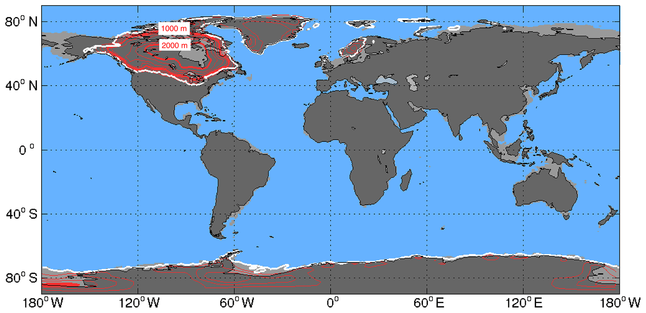
Figure 2 Land–sea mask (light grey/blue shading; dark grey indicates modern land), ice sheet extent (white line) for the MIS3 experiment, and the difference of ice sheet orography relative to PI (red contours with an interval of 250 m; the 1000 and 2000 m isolines are highlighted with bold red lines).

The configuration of global ice sheet extent and height (Fig. 2) is derived from a data-constrained ice sheet model for 38 kyr BP consisting of the Antarctic (Briggs et al., 2014), Greenland (Tarasov and Richard Peltier, 2002), North American (Tarasov et al., 2012), and Eurasian (Lev Tarasov, personal communication) ice sheets. NorESM1-F does not include a dynamic land ice component, and the assumed ice sheet extent and elevation for MIS3 are fixed. The altitude of the land surface is kept at pre-industrial values outside the ice sheet areas. In the areas covered by land ice, the maximum value of the original pre-industrial topography and MIS3 reconstructed ice sheet topography is used; this procedure prevents jumps to high topography adjacent to the ice sheet margin. The resulting MIS3 Laurentide Ice Sheet reaches altitudes higher than 2500 m but is significantly smaller, both in terms of ice extent and height, when compared to the LGM ice sheets such as ICE-6G (Peltier et al., 2015). The southeastern margin of the Laurentide Ice Sheet is further north and the surface is 300–900 m lower than during LGM. Similarly, the Eurasian Ice Sheet is smaller, but there is a significant amount of land ice over Fennoscandia. The Laurentide Ice Sheet is merged with the Cordilleran Ice Sheet in our MIS3 ice sheet configuration. However, the shape of the MIS3 ice sheet is highly uncertain; studies have also shown separated Laurentide and Cordilleran ice sheets before the LGM (e.g. Abe-Ouchi et al., 2007).

For the configuration of land–sea mask in the Barents Sea, care needs to be taken, as this region is an important pathway allowing warm and saline Atlantic water travelling north; therefore, opening or closing it has significant consequences for Arctic ocean circulation and climate (Smedsrud et al., 2013). Unfortunately, there is a lack of reliable geological evidence for the existence of land ice in the Barents Sea before the LGM. However, sparse evidence from the Barents Sea–Svalbard region suggest there was little or no land ice here during MIS3 (Mangerud et al., 1998, 2008; Ingólfsson and Landvik, 2013). Therefore, the Barents Sea is kept free of land ice with a reduced water depth (by 70 m) in the MIS3 configuration of the model. The Canadian Archipelago is covered by land ice, blocking the passage of water between Baffin Bay and the Arctic. In Antarctica, the Ross and Weddell seas are covered by grounded ice rather than floating ice shelves as today.

The land surface vegetation type in the MIS3 configuration is set equal to the pre-industrial values, and the extra land points caused by sea level lowering are assigned as tundra (20 % grass plus 80 % bare ground).

With the adjusted MIS3 land–sea mask and surface topography, a new river-routing map is produced (Fig. S1 in the Supplement). For the ice-free land surfaces, the river routing corresponds to the PI simulation. Where there is new land, due to the lower MIS3 sea level, the river outlets are extended to the ocean. For the ice covered areas, a new map is generated based on the land ice topography, routing the water from the land ice along the steepest gradient, either directly to the ocean or to the nearest river if the ice margin terminates on land.

Salt equivalent to 0.6 g kg⁻¹ is uniformly added to the ocean, to account for the large amount of freshwater stored as ice on land. The vertical coordinate in MICOM is potential density with reference pressure of 2000 dbar and is adapted from a present-day range of 28.202–37.800 to 28.672–38.270 kg m⁻³ below the mixed layer, in order to account for the change in salinity and thus density. As for the PI experiment, the ocean model is initialised with modern temperature and salinity (Steele et al., 2001) with the abovementioned salinity increment applied. Note that no specific protocols on ocean initialisation are defined for glacial simulations; e.g. within the Paleoclimate Modelling Intercomparison Project (PMIP), the groups chose to initialise their models either from present-day conditions or from a glacial ocean state. As illustrated by Zhang et al. (2013), equilibration time for the deep ocean can be significantly reduced (50 % in their model) if a glacial, rather than present-day, ocean state is utilised for initialisation. Note, however, that MIS3 is not a full glacial state and has a climate in between LGM and PI. The PI experiment, that the MIS3 experiment is evaluated against, is performed with the same model, NorESM1-F, and is documented and assessed in Guo et al. (2019). Model equilibration for the NorESM MIS3 experiment will be addressed and discussed in Sect. 3.1.

3 Results

3.1 Model spin-up

The MIS3 experiment was run for 2500 years and the PI experiment for 2000 years. When comparing the two simulations, the model years between 1800 and 2000 are averaged.

Both the PI and MIS3 experiments reach a quasi-equilibrium climate state after the multi-millennial integration, as indicated by the time series shown in Fig. 3. The differences between the global mean MIS3 and PI climate are summarised in Table 2.

Table 2 Global mean values for the MIS3 and PI experiments (both averaged between years 1801 and 2000).

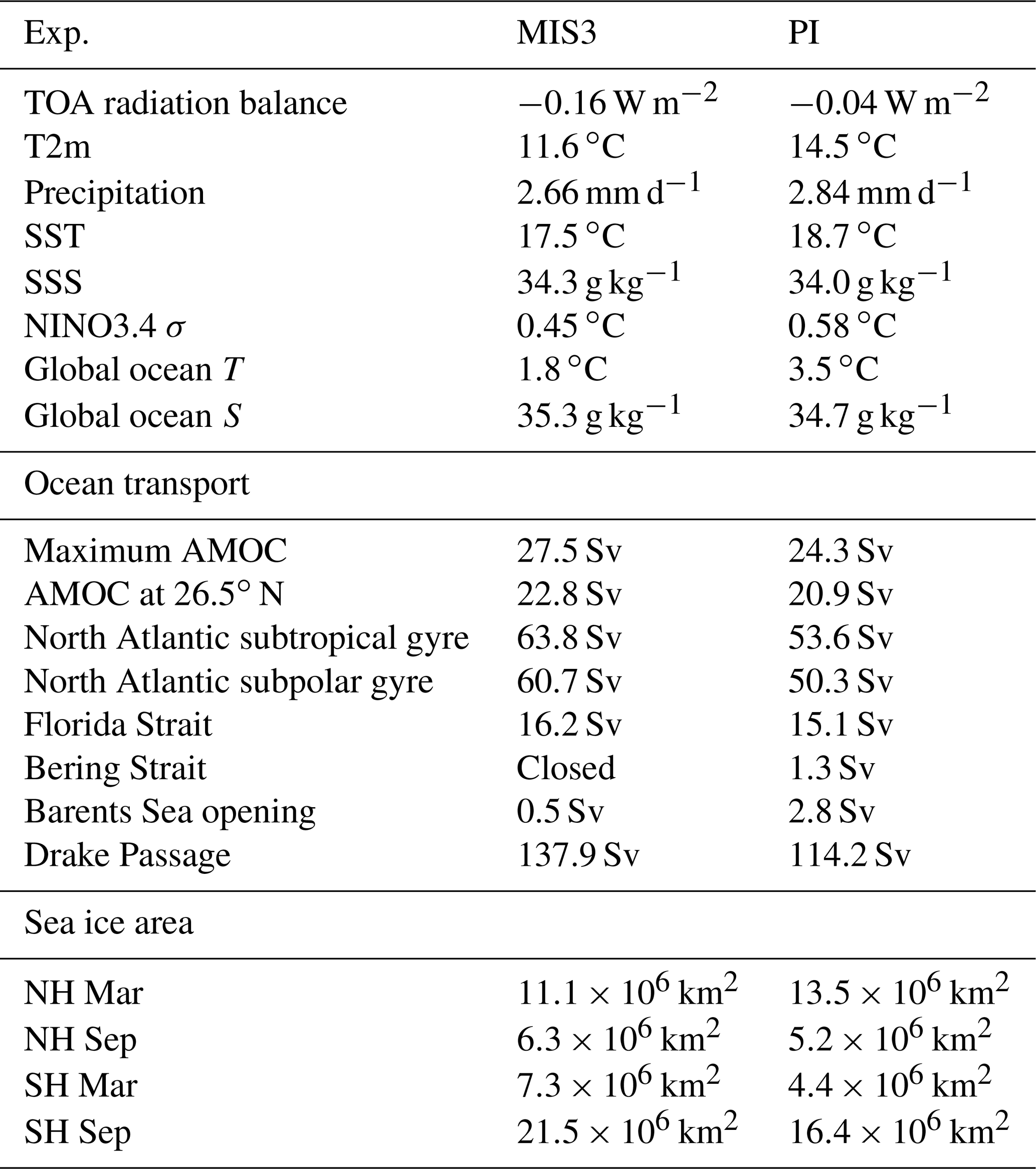
Figure 3 Time series of (a) TOA radiation balance, (b) SST, (c) SSS, (d) global mean ocean temperature, and (e) AMOC strength at 26.5^∘ N for the MIS3 (black) and PI (red) experiments. Light colours denote annual mean values, and dark colours denote 10-year running mean values.

In the following results, the statistical significance of the calculated trends is tested using the Student's t test with the number of degrees of freedom, accounting for autocorrelation, calculated following Bretherton et al. (1999). Trends with p values <0.05 are considered to be statistically significant.

The MIS3 experiment exhibits a small negative TOA radiation balance (−0.16 W m⁻² averaged between model years 1801 and 2000, and −0.08 W m⁻² between 2301 and 2500; Fig. 3a). This results in a negative ocean heat flux at the surface and cooling of the global ocean (Fig. 3d). The cooling trend is −0.05 ^∘C per century over model years 1801–2000 and decreases to −0.02 ^∘C per century over model years 2301–2500; both are statistically significant. Averaged between model years 1800 and 2000, the global mean MIS3 ocean temperature is 1.7 ^∘C colder than that of the PI experiment.

At the ocean surface, sea surface salinity (SSS) in the MIS3 experiment exhibits negligible drift over the model years 1801–2000 (Fig. 3b, c), whereas SST shows a small statistically significant cooling trend of 0.04 ^∘C per century. For MIS3, the global mean SST and SSS are 1.2 ^∘C colder and 0.3 g kg⁻¹ saltier, respectively, compared to the PI experiment. Simulated time evolution of sea ice extent in the Northern and Southern hemispheres shows a small drift towards the end of the evolution (Sect. S1 in the Supplement).

While the simulated MIS3 surface properties reach a quasi-equilibrium state, the ocean interior experiences a multi-millennial cooling trend (Fig. 3d). The slow adjustment of the deep ocean is considered to be important for the evolution of ocean stratification and overturning circulation (Zhang et al., 2013; Marzocchi and Jansen, 2017). As a consequence, care should be taken, and deep ocean equilibration should be assessed. For the deep ocean, the salinity trend in the Atlantic is found to be smaller than 0.006 g kg⁻¹ per century during the model years 1800–2000 (not shown), which is the threshold proposed by Zhang et al. (2013) for an ocean state of quasi-equilibrium.

Both experiments exhibit an increasing AMOC at the beginning of the model integration, followed by a gradual equilibration to a weaker state (Fig. 3e). The simulated pre-industrial AMOC at 26.5^∘ N is 20.9 Sv, which is close to present-day observations (∼18 Sv; RAPID data from http://www.rapid.ac.uk/rapidmoc, last access: 21 June 2019). For the first few hundred years of the MIS3 integration, the AMOC is significantly stronger than in the PI (by up to 10 Sv), but the difference between the two experiments is gradually reduced as the integration continues. Averaged between model years 1801 and 2000, the simulated MIS3 AMOC at 26.5^∘ N is 22.8 Sv, only 1.9 Sv greater than in the PI experiment. Similarly, the simulated maximum strength of the AMOC during MIS3 is 27.5 Sv, 3.2 Sv stronger than that in the PI (24.3 Sv).

The weakening of the AMOC, after the initial overshoot, occurs concurrently with a shoaling of North Atlantic Deep Water (NADW) and more intrusion of Antarctic Bottom Water (AABW) as a manifestation of an adjustment of the deep ocean. Previous studies relate this behaviour to an expansion of Antarctic sea ice in a colder climate (Ferrari et al., 2014; Jansen, 2017): e.g. as Antarctic sea ice grows (Fig. S2), more brine is rejected, favouring the formation of AABW. These processes will be further discussed in Sect. 4.1.

3.2 Simulated MIS3 climate

Atmospheric surface temperature and circulation

Simulated annual mean surface air temperature change with respect to PI is shown in Fig. 4. Significant cooling occurs at high latitudes in both hemispheres. This is particularly clear above the MIS3 Laurentide Ice Sheet, where cooling reaches 25 ^∘C, as well as in the Barents Sea and parts of the Nordic Seas, where sea ice expands (see Fig. 9). The MIS3 experiment also exhibits noticeable cooling over the Kuroshio extension.

Figure 4 Simulated MIS3 minus PI annual mean near-surface air temperature (^∘C).

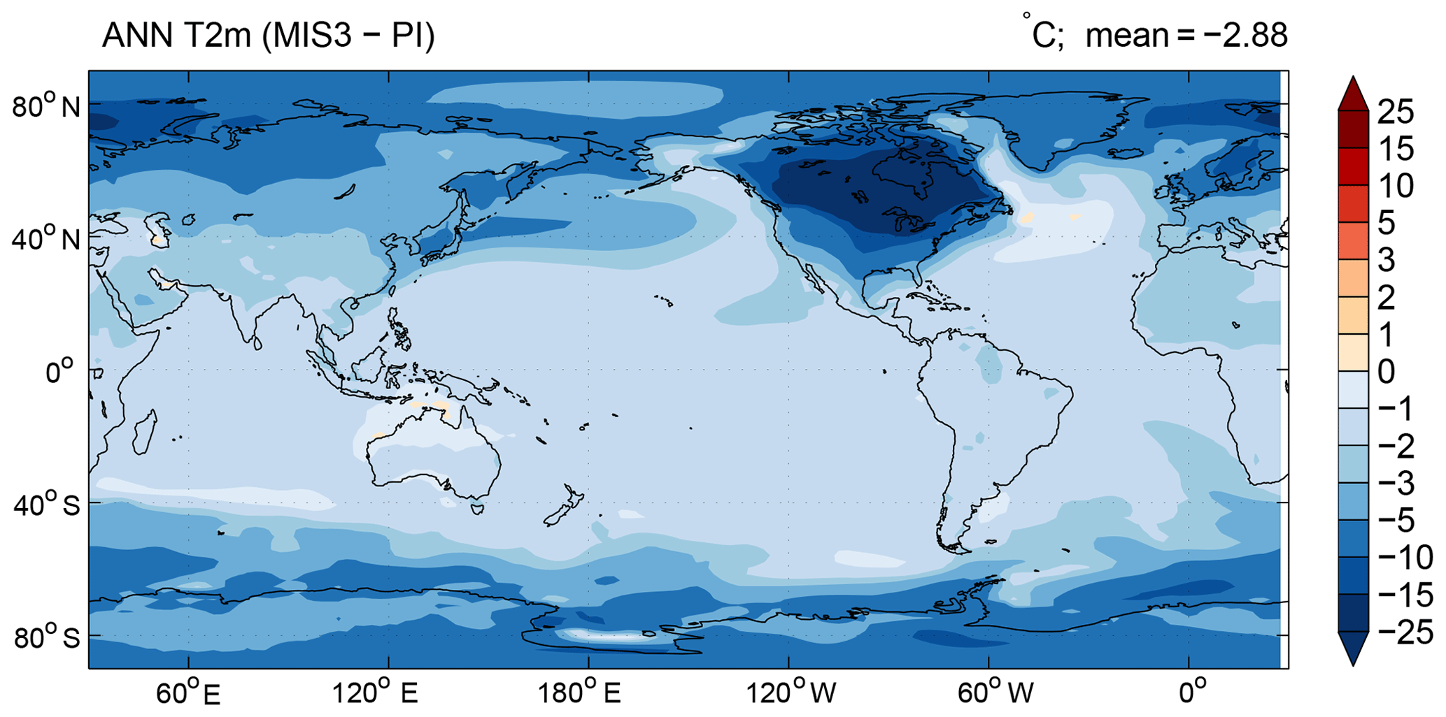
Simulated global mean near-surface air temperature during MIS3 is 2.9 ^∘C cooler than the PI (Table 2). For comparison, the CCSM3 MIS3 simulation (with 35 kyr boundary conditions) by Merkel et al. (2010) showed a cooling of 3.4 ^∘C, whereas using a different version of CCSM3 configured with 38 kyr boundary conditions, Zhang et al. (2014b) reported a cooling of 3.5 ^∘C. A stadial simulation with 44 kyr boundary conditions (Brandefelt et al., 2011) shows a much cooler climate, e.g. 5.5 ^∘C compared to the recent past.

In contrast to the limited number of MIS3 studies, there is a rich literature on the LGM climate. With both similarities as well as apparent differences with regard to the external forcing and the climate, it can be useful to compare the climate of the two periods: our simulated MIS3 cooling is smaller than the reconstructed LGM global mean cooling of 4.0±0.8 ^∘C (Annan and Hargreaves, 2013) and the PMIP2 (Braconnot et al., 2007) and PMIP3 (five models; Braconnot and Kageyama, 2015) simulated LGM cooling range of 3.6–5.7 and 4.4–5 ^∘C, respectively. The simulated cooling during MIS3 is not as intense as that suggested for the LGM, as the continental ice sheets used as forcing are smaller and the atmospheric CO₂ concentration is greater than that during LGM.

The elevated surface of the MIS3 Laurentide Ice Sheet modifies the atmospheric stationary waves, rendering an enhanced, meandering wave pattern in the vicinity of the North American continent (Fig. 5); the displayed 500 mbar geopotential height in winter shows enhanced troughs in the northwestern Pacific and eastern Canada, and enhanced ridges in western Canada. A stronger, more zonal, and northward-shifted (by $\sim \mathrm{4}{}^{\circ }$ in latitude) subpolar jet above the North Atlantic is revealed by the 200 mbar zonal wind (not shown). At the ocean surface, a deepened Aleutian low and the associated development of cyclonic surface wind is found in winter (not shown). The cyclonic wind anomaly advects warm air to Alaska and contributes to the reduced cooling, as seen in Fig. 4. In the Atlantic, a southwestward migration of the Icelandic Low and Azores High leads to broader, stronger, and more southerly located westerlies over the North Atlantic (Fig. 6). The ice-sheet-induced wind anomalies over the North Atlantic are common features also seen in the PMIP3 LGM simulations (Muglia and Schmittner, 2015). The zonal mean NH westerlies (surface zonal wind stress) increase by ∼20 % relative to PI in NorESM and shift equatorward by $\sim \mathrm{4}{}^{\circ }$ in latitude. Furthermore, surface wind stress is significantly increased just off the edge of the sea ice in the Nordic Seas (see Fig. 9) and in the Irminger Sea, possibly caused by the expanded Laurentide Ice Sheet (e.g. Sherriff-Tadano et al., 2018). In the Labrador Sea, a strong northerly wind anomaly is also induced by the nearby Laurentide Ice Sheet.

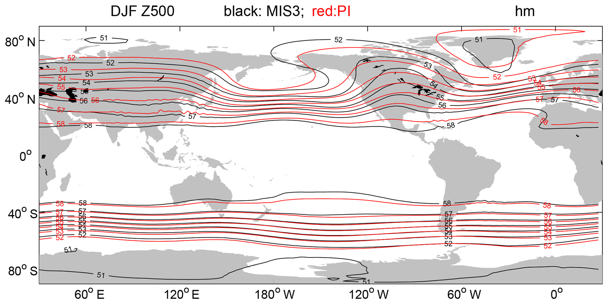
Figure 5 Simulated MIS3 and PI DJF 500 mbar geopotential height (hm). The black and red contours are for the MIS3 and PI experiments, respectively.

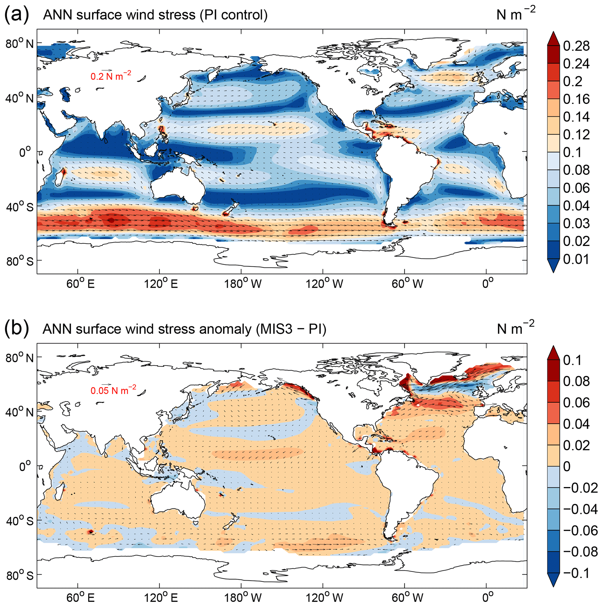
Figure 6 Simulated annual surface wind stress over the ocean for (a) PI and (b) MIS3 minus PI (N m⁻²).

In the tropics, the northeasterly trade winds are strengthened in the NH, while in the SH the southeasterly trade winds are relatively unchanged. In the Southern Ocean, the westerlies are strengthened in the Pacific Ocean sector and weakened in the Indian Ocean sector. The zonal mean of the westerly wind stress in the Southern Ocean shows a slight strengthening during MIS3 (∼4 %), with nearly no latitudinal shift.

In the colder MIS3 climate, simulated global mean precipitation is 0.18 mm d⁻¹ lower, with both seasonal and geographical changes including a southward shift of the Intertropical Convergence Zone (ITCZ) compared to that in PI. More details are given in Sect. S2 in the Supplement.

Ocean circulation and sea surface features

The reduced atmospheric CO₂ concentration during MIS3 causes a lowering of SST and an expansion of sea ice. Simulated global mean MIS3 SST is 1.2 ^∘C colder with respect to the PI. The geographical distribution of the cooling (Fig. 7a) reflects the change in surface air temperature, as shown in Fig. 4. The cooling is relatively modest (1–2 ^∘C) in the tropical and subtropical oceans, and increases towards higher latitudes, in particular in the North Pacific, the Barents Sea, the Nordic Sea, and the Southern Ocean. In contrast, the central North Atlantic exhibits less cooling and even exhibits warming near the centre of the subpolar gyre and at the western rim of the Labrador Sea. While the “warm blob” in the subpolar gyre can be attributed to a shift of the North Atlantic Current at MIS3 (as suggested from the surface velocity and sea level fields; not shown), the relatively weak cooling in the NA subpolar region is likely caused by a stronger AMOC (Fig. 8) and a stronger and slightly more contracted subpolar gyre (Fig. S4) bringing more ocean heat from the tropics to this region (Fig. S5) (Atlantic Ocean heat transport increases by 15 % at 40^∘ N). The overall pattern of weak cooling in the North Atlantic during MIS3 can be compared to the recent 20th century global warming, with a North Atlantic cooling anomaly, suggested to be caused by a reduction in the AMOC (Rahmstorf et al., 2015). The simulated warming along the western rim of the Labrador Sea (1–2 ^∘C), apart from the contribution from a strengthened subpolar gyre (21 % stronger compared to PI), is related to the locally reduced MIS3 sea ice cover (Fig. 9a).

Figure 7 Simulated MIS3 (a) SST and (b) SSS anomalies relative to PI.

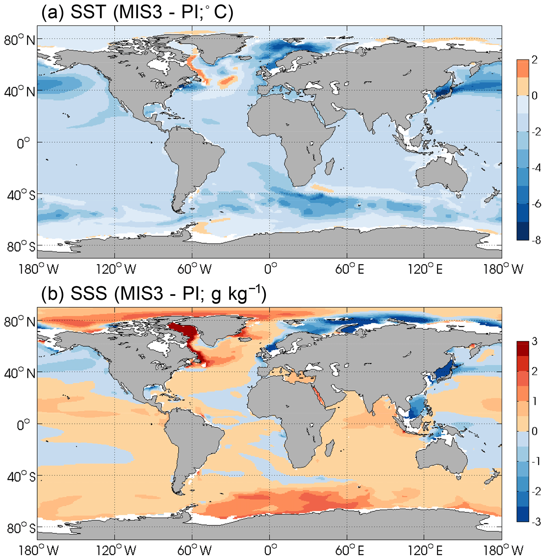
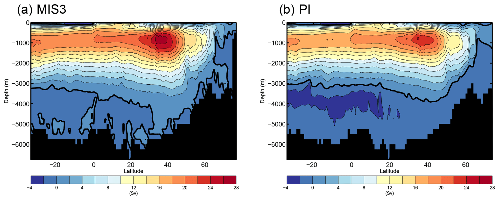
Figure 8 AMOC for (a) MIS3 and (b) PI simulations. The thick black line denotes the zero contour line.

The cooling in the North Pacific is partly associated with a reduction of northward ocean heat transport in this region (Fig. S5); e.g. ocean heat transport is 23 % smaller at 30^∘ N during MIS3. In addition, the cooling is accompanied by expanded winter sea ice cover in the northwestern Pacific (Fig. 9a) and a southward shift of the North Pacific subpolar gyre (Fig. S4).

As northward ocean heat transport in the North Pacific decreases, southward ocean heat transport in the South Pacific and Indian Ocean increases (e.g. 13 % increase at 30^∘ S). Further to the south, the MIS3 simulation shows enhanced meridional ocean heat transport across the Antarctic Circumpolar Current (Fig. S5). However, significant cooling is simulated in this region and is associated with an equatorward expansion of sea ice (particularly in the western Indian Ocean sector; Fig. 9), concomitant with a northward shift of the Antarctic Circumpolar Current (not shown).

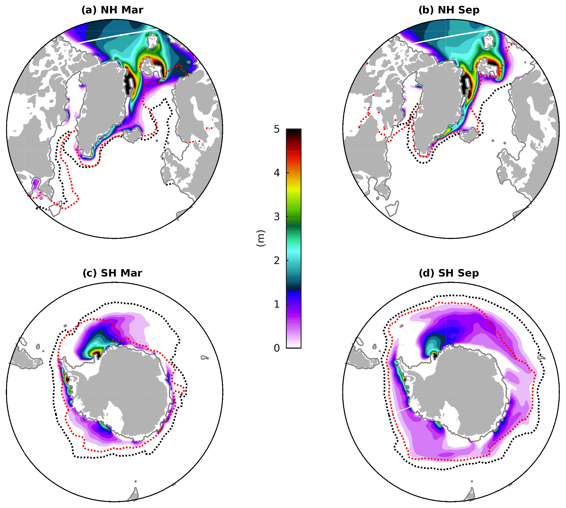
Figure 9 Simulated MIS3 – PI sea ice thickness anomalies (shading; m) for (a) NH March, (b) NH September, (c) SH March, and (d) SH September. Black and red dashed lines denote the 15 % sea ice concentration for MIS3 and PI, respectively. The grey line marks the MIS3 coastline.

For the surface salinity (Fig. 7b), MIS3 is more saline as a result of the addition of 0.6 g kg⁻¹ salt into the global ocean due to expansion of ice on land. Exceptions are the North Pacific subpolar area, South Pacific subtropical area, South China Sea, eastern Atlantic, and off the Eurasian shelf. Strong salinity increases are found in Baffin Bay, the western Labrador Sea, the North American sector of the Arctic, and within and east of the Weddell Sea. The salinity decrease in the North Pacific and salinity increase in the Arctic and in Baffin Bay can be partially attributed to the closure of the Bering Strait (Hu et al., 2010, 2015) at MIS3. The Bering Strait acts as a passage of freshwater from the Pacific to the Arctic Ocean, with an impact on salinity in Baffin Bay and the North Atlantic via the Canadian Arctic Archipelago. The Bering Strait, with a depth of ∼50 m at PI (and at present), is closed due to the lower sea level at MIS3, while the passage through the Canadian Arctic Archipelago is blocked by the presence of expanded MIS3 ice sheets (Fig. 2). A net volume transport of 1.3 Sv low-salinity water, through the Bering Strait in the PI control run (present-day observations are ∼0.8 Sv; Woodgate et al., 2005), is thus removed in the MIS3 run and contributes to the pattern described above.

Dramatic freshening takes place in the Eurasian sector of the Arctic at MIS3. Here, the Arctic river outlets extend further out to the open ocean, relative to the present-day locations, due to the change of land–sea mask (Fig. 2). Such changes in the locations of river outlets, and thus freshwater input, lead to a decrease in salinity, including the region southwest of Norway, where a large glacial river is generated due to the presence of the nearby Fennoscandian Ice Sheet (see Fig. S1). In addition, the volume transport of saline water, of North Atlantic origin, into the Arctic via the Barents Sea opening (from the southern tip of Svalbard to the northern tip of Norway), is reduced from 2.8 Sv at PI to 0.5 Sv at MIS3, contributing to the salinity decrease in the Eurasian sector of the Arctic.

The fresh surface water in the South China Sea during MIS3 is caused by increased runoff from the new river routing in this region due to the change of land–sea mask. In the southwest Pacific, surface freshening is due to a southward shift of the ITCZ and an overall decrease of evaporation minus precipitation in the region. Off the coast of Antarctica, enhanced formation of sea ice (Fig. 9), and the associated brine release, leads to an increase in surface salinity; the effect is especially pronounced in the Weddell Sea region.

AMOC and Atlantic hydrography

Our NorESM experiments show a strengthened AMOC at MIS3 (27.5 Sv) relative to the PI (24.3 Sv) (Fig. 8). The depth of the AMOC maximum for MIS3 is unchanged and located at 800 m. The vertical extent of the AMOC is deepened from 3500 m in the PI to 4200 m at 26^∘ N (present-day RAPID observations give a depth of ∼ 4300 m; Smeed et al., 2016). The deep overturning cell associated with AABW is contracted and weakened. Zhang et al. (2014b) reported a similar strengthening of AMOC during MIS3 (38 kyr boundary conditions), e.g. 15.4 Sv, which is 1.5 Sv stronger than their PI control simulation but is much weaker than our simulated strength of AMOC at MIS3. In contrast to the NorESM simulation, Zhang et al. (2014b) also simulated a shoaling of the AMOC.

Together with the changes to the AMOC, the deep Atlantic ocean exhibits changes in the distribution of water masses. The zonal mean Atlantic (including the Nordic Seas and the Atlantic sector of the Southern Ocean) temperature (Fig. 10a, b) shows that cooling occurs nearly over the entire water column in the Atlantic basin, with the strongest cooling detected near the bottom of the thermocline (>4 ^∘C) and in the deep ocean below 3500 m (1.5–3 ^∘C). The larger temperature decrease in the deep North Atlantic compared to the South Atlantic suggests a more homogeneous deep water distribution in the Atlantic basin with a smaller interhemispheric gradient during MIS3 (Fig. 10b).

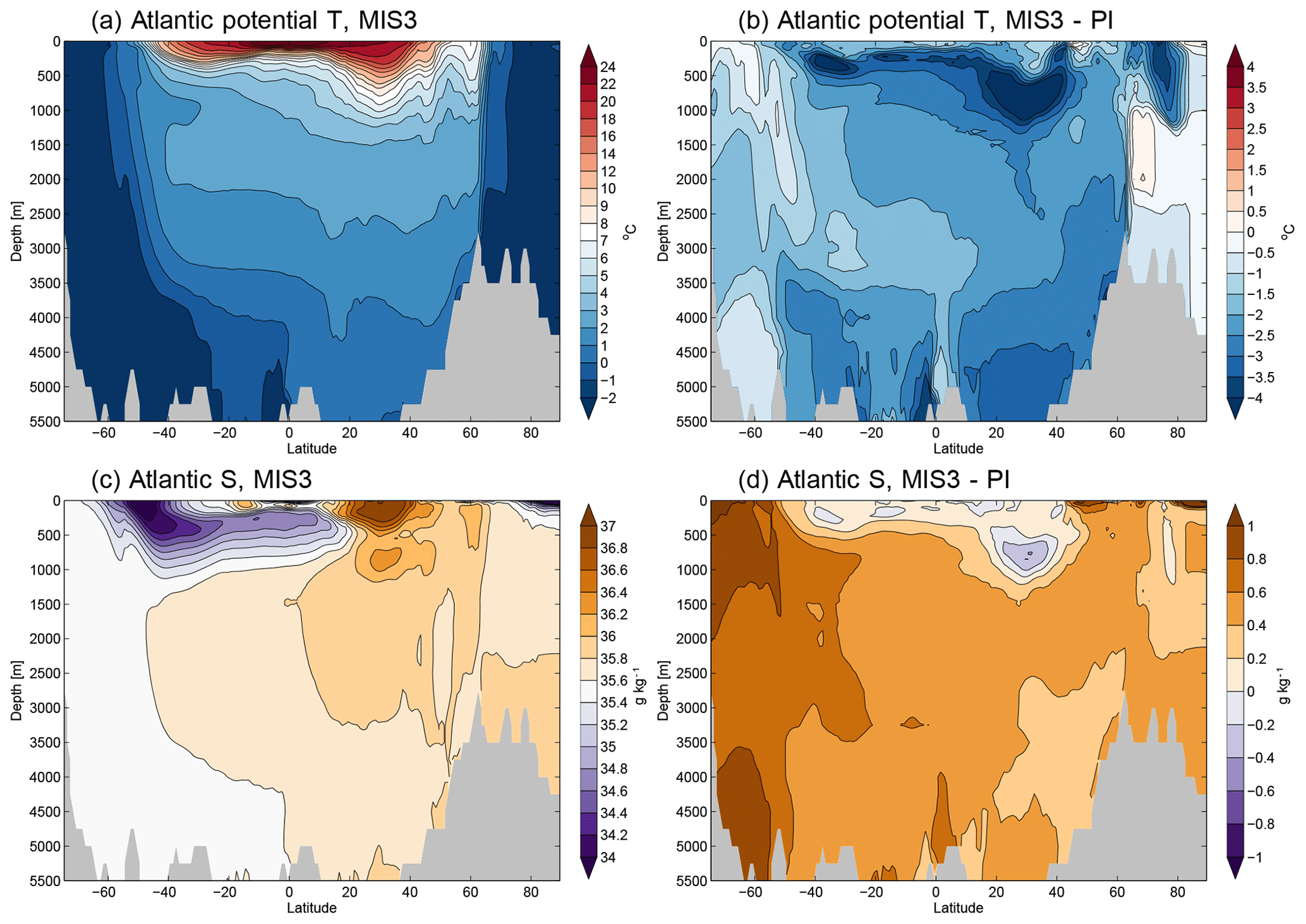
Figure 10 Atlantic zonal mean (a) potential temperature and (c) salinity for the MIS3 experiment and (b, d) anomalies relative to PI.

With more vigorous deep water formation in the NH (associated with a stronger AMOC) and in the SH (as discussed later) during MIS3, enhanced upward motion of sea water is expected away from the sinking regions (Munk, 1966). This leads to a thermocline that is displaced upwards with a sharper vertical gradient, contributing to the cold anomaly near the base of the thermocline as seen in Fig. 10b. Similar upward displacement of the thermocline and an associated cold anomaly are also seen in the Pacific Ocean (not shown). We further note that the cold anomaly centred around 30^∘ N, 500–800 m depth in the Atlantic (Fig. 10b), is primarily caused by reduced warm Mediterranean outflow during MIS3 (not shown).

The Atlantic zonal mean salinity anomaly (Fig. 10c, d) shows an overall increase in salinity, except near the bottom of the pycnocline/thermocline, where the waters are subject to enhanced upwelling as discussed above. Greater freshening is also observed in the saline Mediterranean outflow region where it is reduced during MIS3. For the deeper layers, there is a north–south asymmetry, with more saline bottom water in the South Atlantic (∼0.4 g kg⁻¹) compared to the deep North Atlantic. Geological reconstructions of the glacial deep Atlantic hydrography from pore water measurements suggest a reversed north–south salinity gradient at the LGM (Adkins et al., 2002), e.g. with AABW being more saline than NADW. In our MIS3 simulation, while the gradient is effectively lowered, the reduction is not sufficient to cause a salinity reversal.

In the cold deep ocean, the salinity effect dominates the change of density, manifested by a larger increase of potential density in the Atlantic sector of the Southern Ocean (0.6–0.8 kg m⁻³) compared to that in the Atlantic (0.5–0.6 kg m⁻³) (not shown). A comparison of the ideal age of the water mass (defined as the time since the water mass last made contact with the surface) shows that the Southern Ocean zonal mean ideal age during MIS3 is relatively homogeneous in the vertical and is younger by ∼300 years compared to the PI experiment (Fig. S7), indicating enhanced ventilation of AABW. Kobayashi et al. (2015) reported a similar response of simulated water mass age for the LGM in the Southern Ocean due to enhanced open ocean convections.

Sea ice

As documented by Guo et al. (2019), the PI simulation of sea ice agrees well with observations, both in terms of thickness and extent. The simulated MIS3 sea ice extent and the difference in thickness relative to the PI are shown in Fig. 9. In the NH, MIS3 sea ice is thicker by ∼2 m in the central Arctic in both March and September. In March, sea ice extends further equatorward in the Pacific (reaching 40^∘ N; not shown), and is associated with a cooling in the North Pacific (Figs. 4, 7a) and a southward migration of the Pacific subpolar gyre (Fig. S4).

In the Atlantic at MIS3, there is more winter sea ice south of Newfoundland and in the northeastern Labrador Sea (Fig. 9a). However, there is less sea ice in the western Labrador Sea, which is likely due to the strong northerly katabatic wind induced by the presence of the adjacent Laurentide Ice Sheet (Fig. 6) that moves the ice away. The Nordic Seas are partly ice-covered, with sea ice present off the coast of Norway in winter. However, the central part of the Nordic Seas is ice-free even in winter, due to the intrusion of warm Atlantic water across the Iceland–Scotland ridge. Note that the presence of winter sea ice, in particular in the region southwest of Norway, is not solely governed by the surface climate and inflow of Atlantic water; the simulated nearby river runoff from the Fennoscandian Ice Sheet contributes roughly 0.05 Sv of freshwater input (see also the SSS field in Fig. 7) to the region (about a fourth of the Amazon River discharge), favouring the formation of winter sea ice (Fig. 9a).

In September, the simulated MIS3 sea ice retreats and nearly coincides with PI sea ice extent in the Pacific side (not shown) and in the Labrador Sea (Fig. 9b). Greater sea ice extent is found along the coast of south Greenland and in the Nordic Seas. The Barents Sea is fully ice-covered also in summer at MIS3, in contrast to the PI experiment where this region is seasonally ice-free.

In the SH, MIS3 shows extended Antarctic sea ice cover in both seasons. The seasonal cycle is large in both MIS3 and PI experiments, with the total sea ice area varying by a factor of 3 and 4 between March and September, respectively (Fig. S2; Table 2). Furthermore, sea ice is thicker during MIS3, especially in the Weddell Sea region.

Modes of variability

We briefly evaluate the simulated change of two important climate internal variabilities: the El Niño–Southern Oscillation (ENSO) and the Northern Annular Mode (NAM). Simulated ENSO variability is weakened in the MIS3 compared to the PI simulation. For the NAM, simulated centres of action over the Arctic and North Pacific are both weakened, with the latter much reduced due to the presence of the elevated Laurentide Ice Sheet. More details are given in the Supplement (Sect. S3).

4 Discussion

4.1 Simulated AMOC during MIS3

Abrupt climate changes such as D-O events have been shown to involve changes in both the geometry and strength of the AMOC, as indicated by a number of marine proxy reconstructions (e.g. see the review by Lynch-Stieglitz, 2017) and numerical simulations (e.g. Peltier and Vettoretti, 2014; Brown and Galbraith, 2016). In this study, a stronger and deeper AMOC is simulated during a typical MIS3 interstadial as compared to the PI (Fig. 8). Given its crucial role in the climate of MIS3, we further discuss the simulated AMOC and the associated distribution of NADW and AABW in this section.

Previous studies have argued that the increased production of AABW during glacial times is driven by expanded Antarctic sea ice and enhanced brine rejection during sea ice formation in the Southern Ocean (Shin et al., 2003; Ferrari et al., 2014). The brine induces a negative buoyancy flux, leading to enhanced formation of highly saline AABW (Fig. 10d). Jansen (2017) shows that the changes in the deep ocean stratification and circulation can be interpreted as a direct consequence of atmospheric cooling during glacial times, which induces Antarctic sea ice growth and initiates the processes described above.

The simulated ventilation of AABW is enhanced in our MIS3 simulation compared to the PI (Fig. S7). However, in the Atlantic, the volume of AABW is not comparable with that of the LGM, during which benthic foraminiferal δ¹³C data suggest that AABW dominated the water column in the Atlantic up to a depth of ∼2 km (Curry and Oppo, 2005), together with a shallower NADW production. However, measurements of ²³¹Pa∕²³⁰Th, in combination with ¹⁴³Nd∕¹⁴⁴Nd (ϵ_Nd), indicate that a strong AMOC existed at the LGM despite of a shallow upper cell (Böhm et al., 2015). Böhm et al. (2015) also show that an active AMOC, neither weaker nor shallower than the present day, prevailed over the last glacial cycle, including the D-O interstadials (the exceptions are Heinrich stadials exhibiting weaker and shallower NADW). The AMOC during interstadials is accompanied by active deep water formation in the North Atlantic, with persistent contributions from northern sourced water. Our simulated MIS3 interstadial AMOC agrees with these reconstructions based on chemical tracers, and the difference with the AMOC at the LGM can be partly (if not fully) attributed to less Antarctic sea ice formation due to the MIS3 climate being milder than that at the LGM.

While deep water production in the Southern Ocean has the potential to displace and reduce the strength of the NADW production, competing effects are at play in the North Atlantic. For example, the altered surface westerlies in the North Atlantic caused by the elevated Laurentide Ice Sheet (Figs. 2, 6) are shown to be able to induce a deeper and stronger AMOC by transporting more salt northward within an intensified gyre circulation, favouring deep ocean convection (e.g. Montoya and Levermann, 2008; Oka et al., 2012; Muglia and Schmittner, 2015; Klockmann et al., 2016; Sherriff-Tadano et al., 2018); the closure of Bering Strait leads to an increase of surface salinity in the North Atlantic thereby invigorating deep ocean convection and strengthening the AMOC (Hu et al., 2010, 2015). To isolate and assess the relative impact of these different processes requires a suite of dedicated sensitivity studies which is beyond the scope of this paper, but it is worth mentioning that the processes that take place in both hemispheres act together to create the AMOC shown in Fig. 8.

During the last glacial, sea level lowering and the removal of shallow continental shelves (Fig. 2) result in enhanced tidal dissipation in the open ocean (Egbert et al., 2004), implying enhanced deep ocean mixing and a strengthened AMOC. Schmittner et al. (2015) demonstrated that such tidal effects can dominate over surface buoyancy effects and lead to a strengthening of AMOC by ∼40 %. Such tidal effects are not considered in the current study, but once included, the AMOC is expected to strengthen and deepen, potentially displacing the lower AABW cell in the Atlantic.

4.2 MIS3 simulation forced by typical stadial conditions

The NorESM MIS3 simulation presented above is representative of an interstadial climate, i.e. a relatively warm period during the last glacial; in agreement with paleo-reconstructions, this includes Greenland temperatures only 5–8 ^∘C colder than PI (Huber et al., 2006), a strong and active AMOC (Böhm et al., 2015; Henry et al., 2016), and enhanced sea ice cover in the Nordic Seas (Rasmussen and Thomsen, 2004; Dokken et al., 2013). In particular, using a high-resolution benthic Mg∕Ca temperature record in the Denmark Strait, Sessford et al. (2018) inferred that during the baseline interstadial mode, ocean circulation and the associated water mass properties are similar to the present day; furthermore, a high-resolution reconstruction of MIS3 sea ice, based on analysis of biomarkers from a marine sediment core in the south Nordic Seas (Sadatzki et al., 2019), finds near-perennial sea ice cover during cold stadials, and ice-free periods during warm interstadials. Both proxy studies support our modelled ocean and sea ice state as simulated for the MIS3 interstadial climate state. However, questions remain as to the state of the cold stadial climates of MIS3, which is characterised by much colder Greenland temperatures, near-completely ice-covered Nordic Seas, and reduced AMOC compared to the present day (based on the same references as above). These changes are reinforced during stadials including Heinrich events, when the AMOC shows a further weakening, due to the massive release of icebergs into the North Atlantic (e.g. Henry et al., 2016).

It is unclear if the baseline climate during MIS3 should be a stadial or interstadial state, nor is it clear that there is indeed a baseline climate, as the climate states can be inherently oscillatory (Peltier and Vettoretti, 2014; Brown and Galbraith, 2016; Klockmann et al., 2018). To examine the possibility of simulating a cold MIS3 stadial climate with NorESM, an additional experiment is branched off and initialised from the MIS3 interstadial control experiment after 1700 model years. The MIS3 “stadial” experiment is run for 800 years with 40 kyr orbital forcing and reduced GHG levels (e.g. CO₂ – 200 ppm, CH₄ – 450 ppb, N₂O – 220 ppb) according to Schilt et al. (2010). The major difference compared to the interstadial experiment is that in the “stadial” experiment, the CO₂ is lowered by 15 ppmv.

In the MIS3 “stadial” experiment, the global near-surface temperature cools by 0.4 ^∘C relative to the MIS3 interstadial experiment (Fig. S11). Winter sea ice slightly expands southwards in the Nordic Seas and in the northwestern Pacific, whereas in the Labrador Sea, sea ice distribution is nearly identical in the two experiments. Furthermore, there is a negligible change to the AMOC. Together, these results indicate that given the changes to the GHG levels that are typical of a stadial state, a cold Greenland climate with a weak AMOC cannot be reproduced in our MIS3 setup without additional freshwater forcing.

4.3 MIS3 sensitivity to CO₂ and ice sheet size

With the multi-millennial long integration of the MIS3 simulation presented in this work, only one stable climate state is found, and the model reaches a quasi-equilibrium with a small drift towards the end of the integration. In this section, we explore the potential for model bi-stability associated with the transition between the warm interstadial and cold stadial climate states of MIS3. We do so by perturbing the model with changes in atmospheric CO₂ concentrations and the size of the Laurentide Ice Sheet.

Our NorESM MIS3 simulations agree with that of Van Meerbeeck et al. (2009) using the LOVECLIM model: given MIS3 boundary conditions, the interstadial climate is the equilibrium climate state, whereas the stadial climate is a perturbed state. A CO₂ change of 15 ppmv (typical of stadial conditions) is not sufficient to induce transitions between the two states (Sect. 4.2). However, Zhang et al. (2017) reported that a gradual change of CO₂ concentrations by 15 ppmv in their experiment with intermediate glacial conditions can be sufficient to trigger transitions between weak/strong AMOC modes and therefore stadial/interstadial states. In contrast, Klockmann et al. (2016) examined the effect of CO₂ changes on the AMOC strength and geometry in an LGM setup and found a weakening and shoaling of AMOC with decreasing CO₂ (from 284 to 149 ppmv) but without transitioning into a weak AMOC mode. They argued that the presence of LGM ice sheets could enhance the AMOC by impacting the surface wind stress in their model and thus help maintain the stability of the AMOC. Interestingly, Klockmann et al. (2018) later reported that with a PI ice sheet configuration, the AMOC exhibits oscillatory behaviour at a CO₂ level of 206 ppmv, above (below) which a strong (weak) AMOC mode persists. In addition, the MIS3 simulation reported by Zhang et al. (2014b) is close to disequilibrium and model bi-stability, as indicated by a series of equilibrium freshwater perturbation experiments.

The studies by Klockmann et al. (2016, 2018) and Zhang et al. (2017) on the sensitivity of climate states to CO₂ levels and ice sheet sizes, together with the studies of, e.g. Zhang et al. (2014a), Brown and Galbraith (2016), and Galbraith and de Lavergne (2019), point to the possibility that there could exist a certain range of CO₂ levels and ice sheet sizes in which the model is subject to a mode transition and even excitation of self-oscillatory behaviour in North Atlantic climate. The existence and range of such a “window” of CO₂ levels and ice sheet heights, however, is expected to be model dependent. In order to explore the potential for model climate transition with NorESM and the existence of a cold stadial state given MIS3 boundary conditions, we investigate the model response to large variations of CO₂ and ice sheet height, using the interstadial simulation as the baseline experiment. Another motivation for seeking a cold climate is that, as discussed by Peltier and Vettoretti (2014), a cold Heinrich stadial-like state is required to “kick” the system into a self-oscillatory behaviour. Even without the self-oscillation, a cold stadial state would serve as a useful baseline experiment for investigating potential triggers of the abrupt cold-to-warm D-O transitions.

It is not within the scope of this paper to perform a complete examination of the model response to every combination of CO₂ and ice sheet changes. Rather, we report the model response in the more extreme cases, with a primary focus on the response of the AMOC and sea ice. For the CO₂ sensitivity experiments, we reduce the values from 215 to 160 and 140 ppmv. For the ice sheet sensitivity experiments, we reduce the height of the Laurentide Ice Sheet by 50 % and 100 % (the latter is equal to the pre-industrial orography), while keeping the ice mask unchanged. All the sensitivity experiments are branched off and initialised from the MIS3 interstadial simulation, and all other parameters are kept fixed.

Contrary to the studies cited above, the NorESM MIS3 experiments exhibit surprising stability without any significant changes in Greenland temperature, sea ice, or AMOC (Fig. 11). For the low CO₂ experiments, there is a slight expansion of winter sea ice in the Nordic Seas (Fig. S13), without any notable changes in the strength and locations of convection. As a consequence, the AMOC, although weakened, still remains strong (Fig. 11). For the experiments with a reduced Laurentide ice sheet, surface wind stress fields are altered (mainly shifting northwards in the North Atlantic; not shown), whereas the strength of AMOC is only slightly reduced.

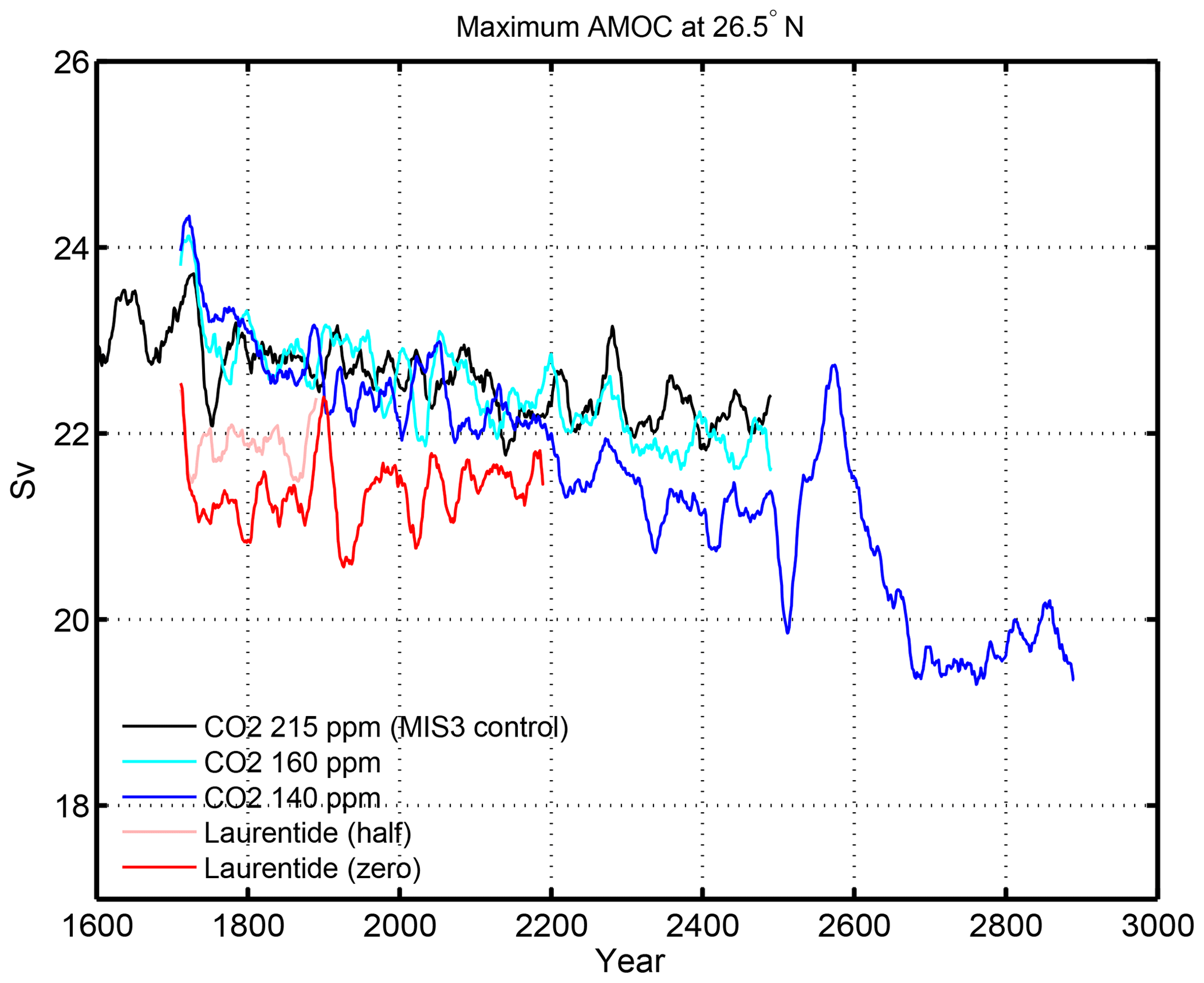
Figure 11 Time series of AMOC at 26.5^∘ N for the experiments with reduced CO₂ levels and reduced Laurentide Ice Sheet heights. The sensitivity experiments are branched off from the MIS3 control run at year 1700 and year 2500, respectively, and the latter are shifted forward by 800 years in the figure.

Further analysis of key relevant metrics, e.g. spatial distributions of SSS, winter sea ice extent, and AMOC geometry for the sensitivity experiments, are included in the Supplement (Sect. S4). As the changes are highly related to the strength of the AMOC, which is only weakly reduced in the sensitivity experiments, changes in these metrics are also relatively small.

The results of the sensitivity experiments to CO₂ and ice sheet height underscore the question of model dependence on the background climate in simulating AMOC transition/bi-stability, despite the fact that the simulations are limited in length (200 to 1000 years), and we therefore cannot fully exclude that further equilibration could bring the climate into a more unstable regime. In our simulation, where the Labrador and Norwegian seas are the major convection sites, a significant change of ocean circulations is not expected unless the Labrador and Norwegian seas are covered by sea ice, thereby inhibiting convection through its insulating effect. However, the NorESM MIS3 and PI experiments both appear to be in a stable regime with a strong AMOC and strong convection in the Labrador and Norwegian seas (Fig. S6). As a consequence, the model state is relatively distant from a potential threshold, including a bi-stability of the AMOC and sea ice. In addition, the NorESM1-F model features a relatively low climate sensitivity (the equilibrium climate sensitivity in response to a doubling of atmospheric CO₂ is 2.3 ^∘C) which plays a role in the weak response of the MIS3 climate to a further CO₂ decrease.

To trigger a cold stadial-like climate state in the NorESM, other mechanisms including enhanced iceberg calving and freshwater input to the North Atlantic from the Laurentide, Greenland and Fennoscandian ice sheets should be considered. There is a rich literature on applying freshwater flux of different magnitudes and locations to study climate response and transitions (e.g. Stouffer et al., 2006; Roche et al., 2010). The prospects of perturbing the MIS3 interstadial climate with freshwater fluxes will be explored in detail in a companion study.

5 Conclusions

In this paper, we present an equilibrium simulation of Marine Isotope Stage 3 forced by 38 kyr BP boundary conditions, with a recently developed version of the NorESM featuring a horizontal resolution of 2^∘ in the atmosphere and 1^∘ in the ocean. The fast performance of the model allows the experiments to be integrated for 2500 years. The boundary conditions are notably different from the pre-industrial due to changes in orbital forcing, greenhouse gases, and the height and extent of the global ice sheets.

The reported simulation, with its current length of integration, does not produce spontaneous transitions between colder stadial and warmer interstadial climate states. Rather, we obtain a MIS3 background climate state with a state-of-the-art climate model that can serve as a baseline for investigating mechanisms behind D-O events by discriminating different factors that can invoke abrupt transitions, e.g. freshwater input, changes in GHG concentrations, ice sheet size, orbital forcing, and ocean diapycnal mixing.

Despite a small drift due to ocean cooling, the model reaches a quasi-equilibrium state in terms of both surface properties and deep ocean hydrography. We analyse the large-scale features of the mean climate states and the model internal variabilities, and compare the results to previous studies of MIS3 and LGM climates. The major findings are as follows:

• Globally, the simulated MIS3 interstadial climate is 2.9 ^∘C cooler than the PI, with amplified cooling in the high latitudes, especially above the ice sheets and near the edges of the newly formed sea ice. The presence of the Laurentide Ice Sheet amplifies the atmospheric stationary waves, leading to an enhanced and northward-shifted jet stream, with stronger and southward-shifted wind stress at the ocean surface.

• The global mean SST at MIS3 is 1.2 ^∘C colder than that at PI, with a pattern of modest cooling in the tropics and enhanced cooling at high latitudes. The North Atlantic subpolar region is characterised by less cooling due to enhanced AMOC and ocean heat transport. Greater cooling is simulated in the North Pacific associated with the expansion of sea ice and southward shift of the subpolar gyre.

• Despite the uniform addition of salt into the global ocean (by 0.6 g kg⁻¹), the distribution of SSS exhibits an inhomogeneous pattern of both salinity increase (e.g. in the central Arctic, the Baffin Bay, and the Weddell Sea region) and decrease (e.g. off the Eurasian shelf, in the North Pacific, and western Pacific and the South China Sea). The closure of the Bering Strait, the increase in sea ice formation, and the change of glacial river routing all play important roles in determining the SSS pattern.

• The upper cell of the AMOC is deepened and intensified under the influence of competing factors from both hemispheres: the cutoff of freshwater input due to the closed Bering Strait and the strengthened surface wind stress in the NH subpolar region both tend to invigorate the AMOC. In the Southern Ocean, expansion of Antarctic sea ice stimulates AABW production by enhanced salt rejection and deep water production. The results are supported by marine proxy records indicating an AMOC comparable to the present day during the last glacial (except during Heinrich stadials). The enhanced deep ocean ventilation in the Atlantic sector of the Southern Ocean leads to reduced (but not reversed) deep north–south salinity gradients in the Atlantic Ocean. The Atlantic displays pronounced cooling below 3000 m in both hemispheres and near the base of the thermocline, the latter due to stronger upwelling of deep water as a result of enhanced deep water formation in both hemispheres. Reduced Mediterranean outflow during MIS3 contributes to the notable cooling and freshening observed around 30^∘ N, 500–800 m depth.

• Sea ice is notably thicker and greater in extent during MIS3 in both hemispheres and seasons. Arctic sea ice is about 2 m thicker and extends further equatorward in the Pacific during winter. The Nordic Seas are partly ice-covered in boreal summer; in winter, sea ice extent is greater but includes an opening in the south due to the intrusion of warm Atlantic water. In the Southern Hemisphere, Antarctic sea ice is thicker (mainly in the western Indian Ocean sector) and extends further north.

• A sensitivity experiment with boundary conditions typical of MIS3 stadial conditions does not reproduce the cold temperatures observed in Greenland, indicating that the interstadial climate in NorESM is relatively stable, and forms the baseline climate during MIS3. Further sensitivity experiments including large changes in atmospheric CO₂ levels and Laurentide Ice Sheet heights, aimed at perturbing the system into a cold stadial-like climate, show that the model is not subject to any bi-stability of the AMOC or sea ice. This underscores the role of model dependency in studying abrupt climate transitions during MIS3 and potentially in the future.