The Late Pliocene jet stream: Changes and drivers of the mean state and variability

Studies of the Late Pliocene have frequently been used as a means to improve our understanding of the climate system in a warmer state. Large scale features of Late Pliocene climate, such as Arctic Amplification, will impact global circulation including the jet stream. To date, the majority of Late Pliocene studies have focused on long term mean climate. However, considering interannual variability is important to fully understand the response of the climate system to different forcings. Using data from the Pliocene Model Intercomparison Project Phase 2, we find a more poleward, yet weaker jet stream in the North Pacific during winter months, and increased interannual jet stream variability in the Late Pliocene compared to the pre-industrial control. This result is consistent across the majority of models, although there is variation in the magnitude of change across the ensemble. Using new simulations from the Hadley Centre Climate Model Version 3 (HadCM3), we find that changes in jet stream variability are due to orographic boundary conditions and are correlated with sea ice feedbacks. Carbon dioxide has little impact on the interannual variability in HadCM3 suggesting that the Late Pliocene is not an analogue for future jet stream variability. This change in jet stream variability in the Late Pliocene could lead to a change in the distribution of temperature and precipitation which could have implications for how proxy data and model simulations are compared.

1 Introduction

1.1 Palaeoclimatology and Late Pliocene climate

As the global climate warms, the frequency and intensity of extreme events have increased, and events are occurring that are outwith the observational record (Robinson et al., 2021). Examining past climates can help the understanding of the behaviour and response of a warmer climate system to different forcings, such as changes to Carbon Dioxide (CO₂) and ice sheet configurations.

One time period well suited to this is the Late Pliocene, specifically Marine Isotope Stage KM5c, 3.205 Ma (within the mid-Piacenzian Warm Period) (Haywood et al., 2024). During this time, both orbital forcing and CO₂ levels (around 400 ppm) were similar to present day values (Haywood et al., 2016; Lan et al., 2025). Reconstructing CO₂ is challenging, so there is an uncertainty on this value, with many strands of proxy evidence. From Boron isotope analysis, De La Vega et al. (2020) report that CO₂ values during the KM5c interval to be ${\mathrm{391}}_{-\mathrm{29}}^{+\mathrm{30}}\mathrm{ppm}$ with 95 % confidence. A value of 400 ppm was chosen for some climate modelling studies to account for the forcing derived from other greenhouse gases that have no proxy reconstructions available (Haywood et al., 2016). Both the Greenland and the Antarctic ice sheets were reduced in size (Dolan et al., 2015; de Boer et al., 2015), leading to higher sea levels (Dowsett et al., 2016). Palaeogeography differs from modern day, including the closure of Northern Hemisphere gateways such as the Bering Strait and the Canadian Archipelago (Dowsett et al., 2016).

Through the Pliocene Model Intercomparison Project (PlioMIP), Late Pliocene climate was simulated by a number of climate models. PlioMIP phase 2 saw 17 climate models complete experiments to understand the behaviour of Late Pliocene climate, and the large-scale features of these simulations are described in Haywood et al. (2020), with the results of HadGEM3 presented separately in Williams et al. (2021). The ensemble multi model mean (MMM) temperature increase from pre-industrial was 3.2 °C with a global increase in precipitation of 7 % (Haywood et al., 2020). Some other significant features of Late Pliocene climate include polar amplification (Haywood et al., 2020), a strengthened Atlantic Meridional Overturning Circulation (AMOC) (Zhang et al., 2021; Weiffenbach et al., 2023) and lower El-Niño variability (Oldeman et al., 2021; Pontes et al., 2022).

To date, the majority of studies focused on the Late Pliocene have looked at changes to the mean state. As the Late Pliocene gains momentum as a potential analogue for the future (Burke et al., 2018; Burton et al., 2025), and to improve our understanding of the climate during this time, it becomes important to consider higher-frequency variability. Considering variability and extremes within a palaeoclimate context could provide important considerations for the interpretation of both proxy and climate model data. In climate projections, distributions of temperature and rainfall shift, with more extremes expected (Kodra and Ganguly, 2014; O'Gorman, 2015). It can be assumed that these distributions were also skewed, compared to pre-industrial, in past warmer climates like the Late Pliocene.

Obtaining well-dated proxy data at the temporal resolution needed to perform analysis on extreme events is challenging. It is therefore important to understand the drivers of extreme events and examine how they change, using climate models, before thinking about how they could occur in the proxy record. Furthermore, looking at extreme events in simulations of a warm climate where the mean state has been validated against proxy data (McClymont et al., 2020; Tindall et al., 2022), can help us understand how climate models represent large scale climate features. Understanding the large scale features, and how well a model captures them, is a necessary first step to understanding the variability, extremes and their drivers seen in the climate system.

1.2 Jet stream controls variability and its relationship to extremes

One key feature in the mid-latitudes that can impact extreme events is the jet stream. Jet streams are fast-flowing, narrow bands of air in the upper troposphere. In each hemisphere, there are two main jet streams, the polar jet which forms at the polar front, and the sub-tropical jet which forms at the upper boundary of the Hadley Cell. These jet streams form in response to meridional temperature gradients and the Coriolis Force (Woollings, 2010).

As observations and climate projections show an amplified rate of warming in Arctic surface temperatures (Rantanen et al., 2022; McCrystall et al., 2021), the surface meridional temperature gradient is reduced. This would suggest an equator-ward shift in the jet stream. Despite this surface change, the jet has been observed to be shifting polewards and becoming more wavy (Martin, 2021). Woollings et al. (2023) link this trend to an increase in meridional temperature gradient in the upper troposphere, with changes to the tropopause height also being important for jet stream dynamics (Lorenz and DeWeaver, 2007).

Many other factors can impact jet stream behaviour both globally and regionally. For example, the topography of the Greenland Ice Sheet can influence the North Atlantic jet (White et al., 2019). Sea ice cover has also been related to changes in mid-latitude circulation. Decreasing sea ice cover is linked to an equatorward shift in the jet stream in future projections, which could inhibit the poleward shift of the jet stream in future climate (Zappa et al., 2018; Screen et al., 2018). Feedbacks in the climate system from sea ice loss are also an important factor to consider when thinking about Arctic influence on the jet stream. Observational studies show links between sea ice loss and changes to cold season weather in the mid-latitudes (Cohen et al., 2014; Overland et al., 2015), although short observational records make it difficult to draw statistically significant conclusions from them. The same connection is debated in modelling studies with some studies finding no link (Cohen et al., 2019) and other studies finding weak, but significant links (Smith et al., 2022).

Shifts in the jet stream may lead to changes in the occurrence of extreme events in the mid-latitudes. Jet waviness has been linked to changes in extreme weather, although this is regionally dependent (Röthlisberger et al., 2016). This is a similar result to a study finding that jet stream tilt produces different regional responses over the European region (García-Burgos et al., 2023). The relationship between the jet and mid-latitude winter extremes can also be related to atmospheric blocking (Sillmann and Croci-Maspoli, 2009; Buehler et al., 2011), with atmospheric blocking being associated with Rossby wave breaking (Pelly and Hoskins, 2003).

It is clear that no one change in the climate system is solely responsible for changes in jet stream behaviour, and is in response to a combination of forcings, which palaeoclimatology may be well placed to investigate.

1.3 Jet stream in the Late Pliocene

To date, a few studies have investigated the behaviour of the jet stream during the Late Pliocene. Li et al. (2015) looked at mean state changes to the westerly winds across the mid-Piacenzian Warm Period with data from PlioMIP1 and found that the westerly winds were displaced poleward compared with the pre-industrial. A difference was noted in the response of the atmosphere-only and coupled ocean–atmosphere models, with ocean–atmosphere models exhibiting a smaller polar shift compared to the atmosphere only models. This highlights the importance of ocean heat transport and sea ice dynamics on mid-latitude circulation. As PlioMIP2 provided new boundary conditions, including the closure of Arctic Ocean gateways, leading to a better data-model comparison in the higher latitudes (Haywood et al., 2020), the PlioMIP2 ensemble will likely provide more insights into circulation changes in the Late Pliocene, relative to PlioMIP1.

Work has also been carried out looking at the drivers of jet stream change and variability. Using CCSM4-UoT it was noted that CO₂ had little impact on changes to the jet stream and that ice sheet and orography changes were more significant in the generation of a wave train (Menemenlis et al., 2021), although the forcing decomposition employed was not full as suggested by Lunt et al. (2021), that may neglect nonlinearities. Oldeman et al. (2024) also investigated jet stream variability in the North Pacific and found that in the Pliocene the jet stream was weaker and more variable in position due to increased Rossby wave breaking. It was also found that non-CO₂ boundary conditions created the majority of the differences. Both of these studies only used one climate model in their analysis and may not capture the true change in the jet stream, as the representation of the jet stream varies between models due to model resolution and how drag is parameterised (Zappa et al., 2013; Pithan et al., 2016).

One challenge in examining changes to jet stream behaviour in the Late Pliocene is the lack of a direct proxy for jet stream behaviour to perform data-model comparisons. However dust flux proxies can be used to reconstruct past atmospheric circulation (e.g. Abell et al., 2021), and more proxy derived information about interannual variability in the Pliocene may be available in the future. For this study we note that mean Pliocene climate variables have been reconstructed from proxy data (e.g. McClymont et al., 2020), hence Pliocene model simulations have a level of data validation that is not possible for future studies. This means that understanding modelled jet stream behaviour in the Pliocene can indicate how the jet stream may have responded to a real world warm climate, and can contribute to our overall understanding of the jet stream and how it is modelled.

This study aims to examine Late Pliocene jet stream change, in the mean state and monthly variability, to understand more about the climate system from a multi-model perspective. We also present new HadCM3 simulations with an aim to understand the drivers of the change. This will provide a perspective on the usefulness of the Late Pliocene as a past analogue for future jet stream variability. Details of the simulations and analysis techniques used are in Sect. 2. Section 3 contains the results and an interpretation of the mean state jet, the variability in the jet stream and explores the roles of different forcing to the changes observed. In Sect. 4, we then provide a perspective on how future studies can build upon this work, enabling a deeper understanding on Late Pliocene climate, and how that can help inform future changes in the climate system.

2 Methods

2.1 Model simulations and data

2.1.1 The PlioMIP2 ensemble

The PlioMIP2 ensemble consists of simulations completed by 17 coupled climate models. Each model contributes to the core experiments, a pre-industrial control simulation (E²⁸⁰) simulation and a Late Pliocene simulation (Eoi⁴⁰⁰) simulation following the PlioMIP2 experimental design (Haywood et al., 2016). Here we follow the naming convention used in PlioMIP2 (Haywood et al., 2016). In the experiment names, “o” indicates Late Pliocene orography (including land–sea mask and vegetation), “i” indicates Late Pliocene ice sheets and the number represents the CO₂ value used.

This means that the E280 simulation has pre-industrial orography and ice sheets with CO₂ at 280 ppmv, while the Eoi⁴⁰⁰ simulation has Pliocene orography and ice sheets with CO₂ at 400 ppmv. Both experiments have non-CO₂ greenhouse gases set as pre-industrial. Pliocene ice sheets (in Eoi⁴⁰⁰) are reduced relative to pre-industrial over Greenland and Antarctica, while Pliocene orography includes closed northern hemisphere ocean gateways (Canadian Archipelago, Bering Strait and Hudson bay) and changes to vegetation. The boundary conditions used in each experiments are in Table 1, where we also include the PlioMIP3 names for ease of comparison to future studies. A full description of the boundary conditions and experimental design can be found in Dowsett et al. (2016) and Haywood et al. (2016).

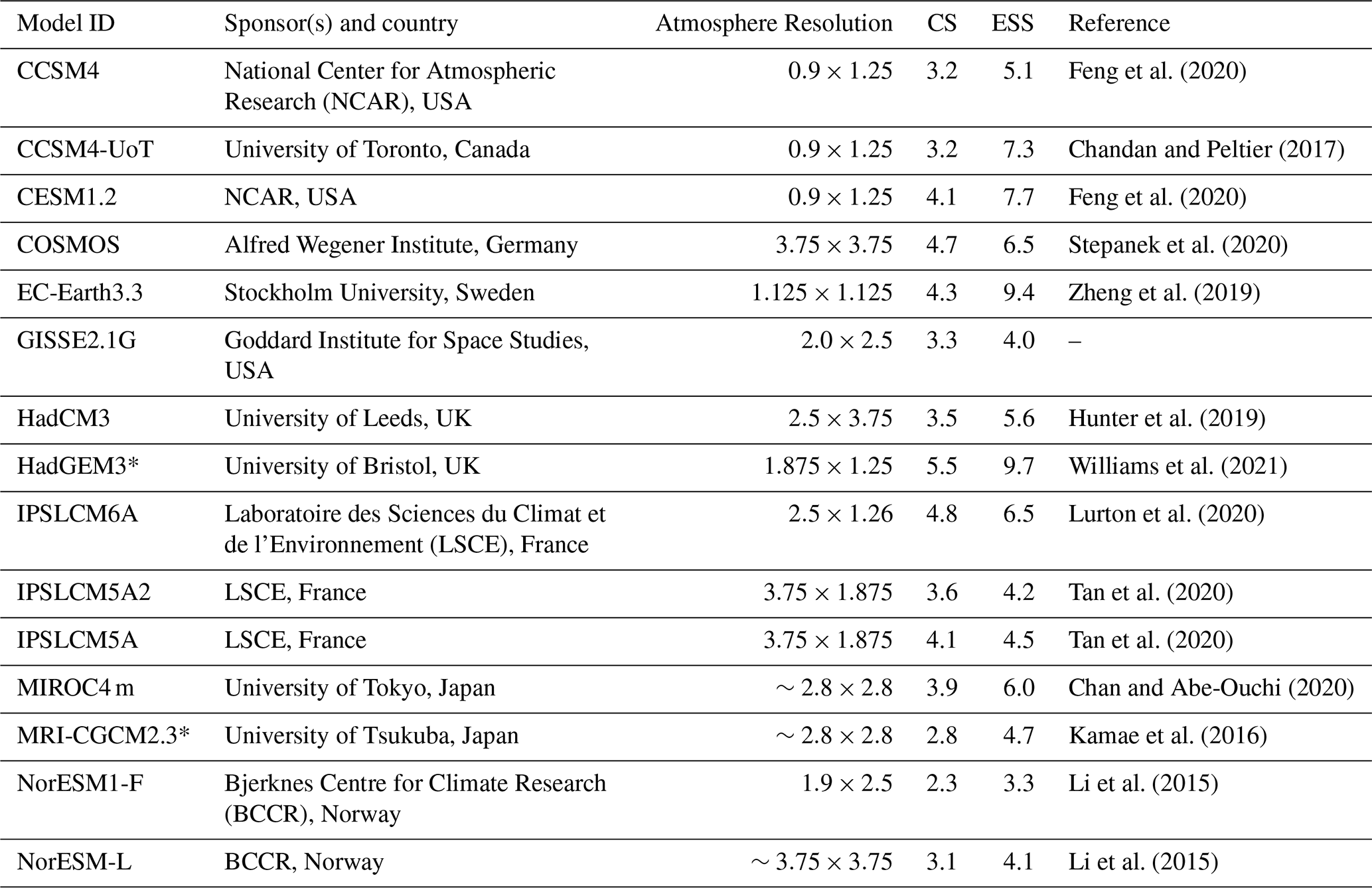
The boundary conditions used in each experiment are in Table 1. We also include the PlioMIP3 names for ease of comparison to future studies. The 15 PlioMIP2 models used to examine the mean state behaviour in this paper are found in Table 2. Two models in the PlioMIP2 ensemble, CESM2 and CCSM4_Utrecht, are not examined here due to difficulties in regridding to a common grid.

Table 1 Boundary conditions from a selection of PlioMIP2 runs. These simulations are set up following the PlioMIP2 guidance (Haywood et al., 2016) and overlap with the PlioMIP3 experimental design (Haywood et al., 2024). We include the experiment names for both PlioMIP2 and PlioMIP3 to allow for comparison between both phases. Here, orography also includes vegetation and land–sea mask changes.

Feng et al. (2020)Chandan and Peltier (2017)Feng et al. (2020)Stepanek et al. (2020)Zheng et al. (2019)Hunter et al. (2019)Williams et al. (2021)Lurton et al. (2020)Tan et al. (2020)Tan et al. (2020)Chan and Abe-Ouchi (2020)Kamae et al. (2016)Li et al. (2015)Li et al. (2015)

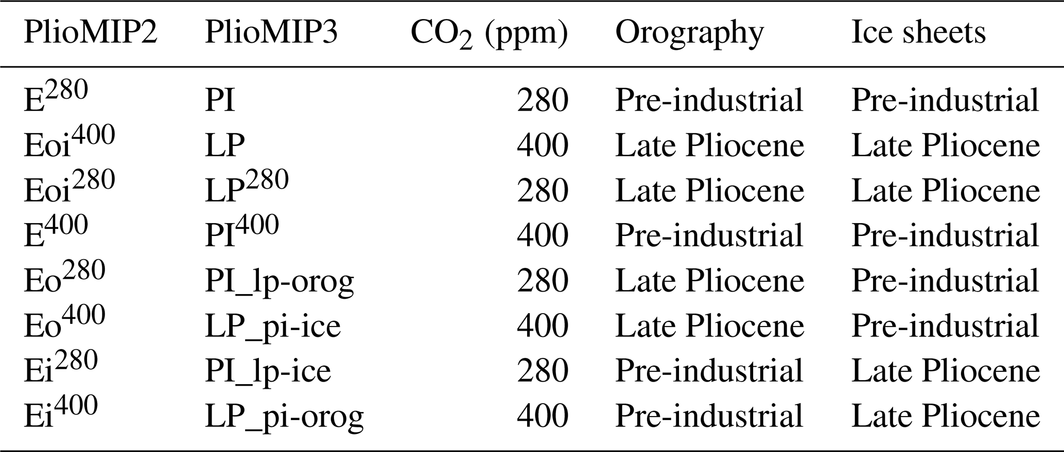
Table 2 The PlioMIP2 models used in this study. The Climate Sensitivity (CS) and Earth System Sensitivity (ESS) are taken from Haywood et al. (2020) and Williams et al. (2021). Models with an asterisk (*) use the land sea mask of the pre-industrial control simulation (E²⁸⁰) for the Late Pliocene (Eoi⁴⁰⁰) experiments.

2.1.2 New model simulations using HadCM3

To disentangle the contributions of change in the jet stream from CO₂, ice sheet and orography forcings, four new forcing factorisation experiments using the Hadley Centre Model Version 3 (HadCM3) were used. These simulations form part of the HadCM3 contribution to PlioMIP3. For a description of the model structure see Gordon et al. (2000) and updates in Valdes et al. (2017).

HadCM3, a coupled atmosphere–ocean general circulation model, has been extensively used for palaeoclimate studies including simulations of the Pliocene (e.g. Hunter et al., 2019). Due to a runtime of 50–100 model years per day, it can be run for long enough that the climate can reach an equilibrium state. The atmosphere component has a horizontal resolution of 3.75° longitude by 2.5° latitude, with 19 vertical layers and a 30 min time step. This makes it one of the lower resolution models within the PlioMIP2 ensemble (Table 2). It simulates a Late Pliocene warming of 2.9 °C, close to the MMM (3.2 °C), within the model range (5.2–1.7 °C) and is in reasonable agreement with proxy reconstructions (Haywood et al., 2020). The model is run with prescribed static vegetation and uses the MOSES2.1 land surface scheme.

The ocean is a rigid-lid model with a horizontal resolution of 1.25° by 1.25° and 20 unevenly spaced vertical layers with a time step of one hour, which is coupled to the atmosphere at the end of each model day. Each atmospheric grid cell is associated with 6 ocean cells, meaning that the coastlines in the ocean surface layer have a resolution that matches the atmospheric component. For further information on the setup of HadCM3 for PlioMIP2 see Hunter et al. (2019).

To set up the forcing factorisation experiments (Eo²⁸⁰, Ei²⁸⁰, Eo⁴⁰⁰, Ei⁴⁰⁰), the PlioMIP2 experimental design in Haywood et al. (2016) was followed. These experiments have also been retained as optional experiments in PlioMIP3 (Haywood et al., 2024). It was decided to produce the full suite of forcing factorisation to be able to achieve a full forcing factorisation as described by Lunt et al. (2021). There is a slight divergence from the original protocol, the enhanced Late Pliocene boundary conditions were implemented, as opposed to the standard Late Pliocene land–sea mask. The enhanced boundary conditions contain the full palaeogeographic reconstruction, whereas the standard boundary conditions retain a modern land–sea mask with the exception of closing the Hudson Bay, Bering Strait and Canadian Archipelago. The enhanced boundary conditions were implemented to be more comparable with the other experiments.

The forcing factorisation experiments were constructed by combining the boundary conditions and initial conditions (ocean temperature and salinity) from other PlioMIP2 experiments (E²⁸⁰, E⁴⁰⁰, Eoi²⁸⁰ and Eoi⁴⁰⁰). For experiments with pre-industrial ice sheets and Late Pliocene orography, the boundary and initial conditions outside of the ice sheet regions from the Late Pliocene runs were used, and the ice regions were changed to match the pre-industrial boundary conditions. The same approach was used for experiments with Late Pliocene ice sheets and pre-industrial experiments. One limitation of this setup is that it does not fully separate the impact of ice sheets from orography as changing the ice sheets requires changes to the orography and vegetation within the ice sheet regions. The experiments were branched off at model year 3500 from fully spun up from HadCM3 PlioMIP2 experiments and ran for a further 3500 to allow for the climate to reach an equilibrium state (measured by top of atmosphere radiation balance). These experiments were run using the same model parameters as the PlioMIP2 runs presented in Hunter et al. (2019). As the experiments were branched off from fully spun up runs, and ran to equilibrium, the results are comparable between the forcing factorisation experiments and the pre-existing simulations presented in Hunter et al. (2019).

2.1.3 The Lunt et al. (2021) factorisation method

These new simulations can be combined with existing experiments (E²⁸⁰, Eoi⁴⁰⁰, E⁴⁰⁰ and Eoi²⁸⁰) to allow for a full forcing factorisation to be completed. To separate out the contribution of each of the factors listed in Table 1 on the Late Pliocene climate we employ the linear-sum factorisation developed by Lunt et al. (2021):

$$\begin{array}{}\text{(1)}& {\displaystyle }& {\displaystyle }\begin{array}{rl}{\displaystyle }\mathrm{\Delta }{x}_{\mathrm{1}}& {\displaystyle }=\mathrm{1}/\mathrm{6}\left[\mathrm{2}\right(x_{\mathrm{100}}-x_{\mathrm{000}})+(x_{\mathrm{110}}-x_{\mathrm{010}})\\ {\displaystyle }& {\displaystyle }+(x_{\mathrm{101}}-x_{\mathrm{001}})+\mathrm{2}(x_{\mathrm{111}}-x_{\mathrm{011}})]\end{array}\text{(2)}& {\displaystyle }& {\displaystyle }\begin{array}{rl}{\displaystyle }\mathrm{\Delta }{x}_{\mathrm{2}}& {\displaystyle }=\mathrm{1}/\mathrm{6}\left[\mathrm{2}\right(x_{\mathrm{010}}-x_{\mathrm{000}})+(x_{\mathrm{110}}-x_{\mathrm{100}})\\ {\displaystyle }& {\displaystyle }+(x_{\mathrm{011}}-x_{\mathrm{001}})+\mathrm{2}(x_{\mathrm{111}}-x_{\mathrm{101}})]\end{array}\end{array}$$

$$\begin{array}{}\text{(3)}& {\displaystyle }{\displaystyle }\begin{array}{rl}{\displaystyle }\mathrm{\Delta }{x}_{\mathrm{3}}& {\displaystyle }=\mathrm{1}/\mathrm{6}\left[\mathrm{2}\right(x_{\mathrm{001}}-x_{\mathrm{000}})+(x_{\mathrm{101}}-x_{\mathrm{100}})\\ {\displaystyle }& {\displaystyle }+(x_{\mathrm{011}}-x_{\mathrm{010}})+\mathrm{2}(x_{\mathrm{111}}-x_{\mathrm{110}})]\end{array}\end{array}$$

where x is the climate variable of interest and the subscript represents the combination of CO₂, ice sheets, and orography used in that simulation. 1 represents Late Pliocene conditions and 0 represents pre-industrial conditions. For example, x₁₀₀ would be the experiment with Late Pliocene CO₂ but with pre-industrial orography and ice sheets, the E⁴⁰⁰ experiment. x₀₁₀ would represent the Ei²⁸⁰ experiment with pre-industrial CO₂ and orography, but Late Pliocene ice sheets. This factorisation is complete, unique, pure and symmetric (Lunt et al., 2021).

2.1.4 Reanalysis data

ERA5 reanalysis data (Hersbach et al., 2023) is used to understand how well the pre-industrial control model simulations capture observations. ERA5 reanalysis data uses data assimilation from observations in combination with a model to provide a record of global atmospheric conditions (Hersbach et al., 2020). ERA5 data spans from 1940 to the present, producing a record shorter than the modelling runs presented here which may impact some of the variability metrics. Therefore, data from the NOAA–CIRES–DOE Twentieth Century Reanalysis version 3 (NOAA CR20) is also included here, as the record begins in 1806 (here we use data beginning in 1916). NOAA CR20 only incorporates surface based observations which can lead to bias in the upper atmosphere (Slivinski et al., 2021). The reanalysis data will also contain influences of anthropogenic climate change, so is not a perfect comparison to model runs in climate equilibrium, however reanalysis data becomes less reliable the further back in time due to limited data sources so the more recent reanalysis data is used. Therefore, there is also potential for uncertainty in the comparison of the PlioMIP2 control runs to reanalysis data.

2.2 Analysis of model simulations

For the analysis, we take the final 100 years of each simulation and use the zonal wind speed and temperature fields at different pressure levels in the atmosphere. The model data was bi-linearly regridded to a 1° by 1° grid to allow for comparison between models and to construct a MMM.

Here we define the jet stream using the maximum zonal wind speeds. Following the methods employed by Li et al. (2015), the latitude of the jet stream is defined as the latitude of maximum zonally averaged zonal wind, and the speed is taken as the maximum speed of the zonal wind. Although taking a single maximum may remove any zonal variability in position, it is sufficient for this study examining monthly averages. As in Li et al. (2015), the zonal wind is examined on three pressure levels (850, 500 and 200 hPa). The analysis of the variability is concentrated at the 200 hPa level as all the models studies present data on this level, and the impact of the vertical movement of the jet is minimal (Fig. S1 in the Supplement). The latitude of maximum speed is found by performing a cubic spline interpolation around the points of maximum speed to achieve a latitude to 0.1°. As the jet stream and its impacts are regionally dependent, we study North Pacific and the North Atlantic separately to improve how. The North Atlantic region is defined as 15–75° N, 60° W–0° E following Woollings et al. (2010). We define the North Pacific region as 15–75° N, 160–220° E to be consistent with previous Pliocene studies of North Pacific jet stream variability (Oldeman et al., 2024). To understand the mechanisms of change we use the Lunt et al. (2021) method described in Sect. 2.1.3 on the zonal wind speeds and upper level temperature change. We focus on Northern Hemisphere winter (December, January and February, DJF) for this analysis as the jet stream is strongest during this time due to an increased meridional temperature gradient. Similar analysis could be repeated for the Southern Hemisphere, but is not done so here to allow for more focused analysis on one region.

To measure the variability of the jet stream latitude (referred to as jet stream variability), we calculate the standard deviation of the latitude of maximum wind speed in the month of January at 200 hPa. Focusing on one pressure level will not account for the vertical displacement of the jet stream, but this vertical displacement was found to have little change on the results in HadCM3 (Fig. S1). As the surrounding pressure levels are not common to all the model output we chose to focus on one level to include as many models as possible in the variability analysis. Only one month was studied for the variability metrics to not smooth any changes in latitude across a season. The variability analysis is focused on the North Pacific, as a persistent wave breaking pattern in the North Atlantic and the presence of a double peak in some of the models complicated the analysis.

3 Results and interpretation

3.1 Changes to the mean state jet stream

Unlike previous studies on the Late Pliocene jet stream that consider global zonal averages (Li et al., 2015), the behaviour of the zonal winds is studied separately for different regions. In the North Pacific region, the pre-industrial control MMM captures the reanalysis well (Fig. 1). In the simulations, the zonal wind speeds are reduced in the Late Pliocene compared to the pre-industrial with a slight poleward shift seen in the MMM (Fig. 1). The MMM poleward shift of the latitude of maximum zonal wind speed is 0.6, 1.8 and 2.0° at 200, 500 and 850 hPa respectively. This is in line with the expected response due to weakening of the meridional temperature gradient reported in the PlioMIP2 ensemble (Haywood et al., 2020).

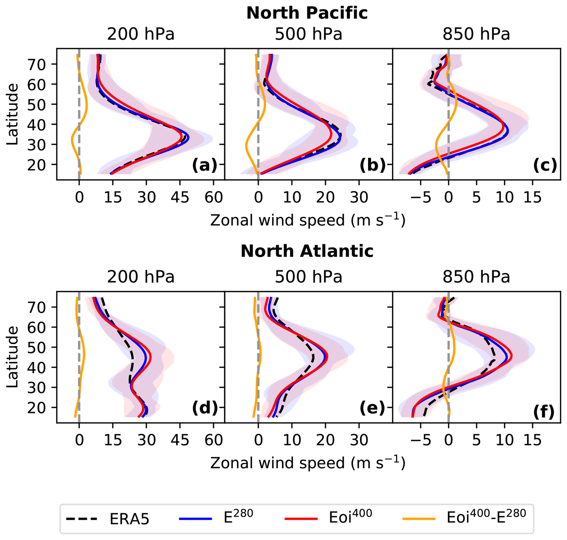
Figure 1 Boreal winter (DJF), multi-model mean zonal wind speeds for the pre-industrial (E²⁸⁰), Late Pliocene (Eoi⁴⁰⁰) and the anomaly (Eoi⁴⁰⁰–E²⁸⁰). ERA5 reanalysis data is shown in the dashed black line. (a–c) is for the North Pacific region and (d–f) is for the North Atlantic. Shading represents the multi model range.

Although the MMM shifts, the range of model response can not be ignored. As demonstrated in Figs. 1 and 2, the models feature a large range of possible jet stream changes. Eight of the models agree with a poleward shift at 200 hPa and 13 of the 15 models agree with a poleward shift in at least one pressure level (Fig. 2). Each model in the ensemble captures the general feature of the jet stream when comparing the pre-industrial control simulation against ERA5 reanalysis data, although some models are a closer fit than others (Fig. S2).

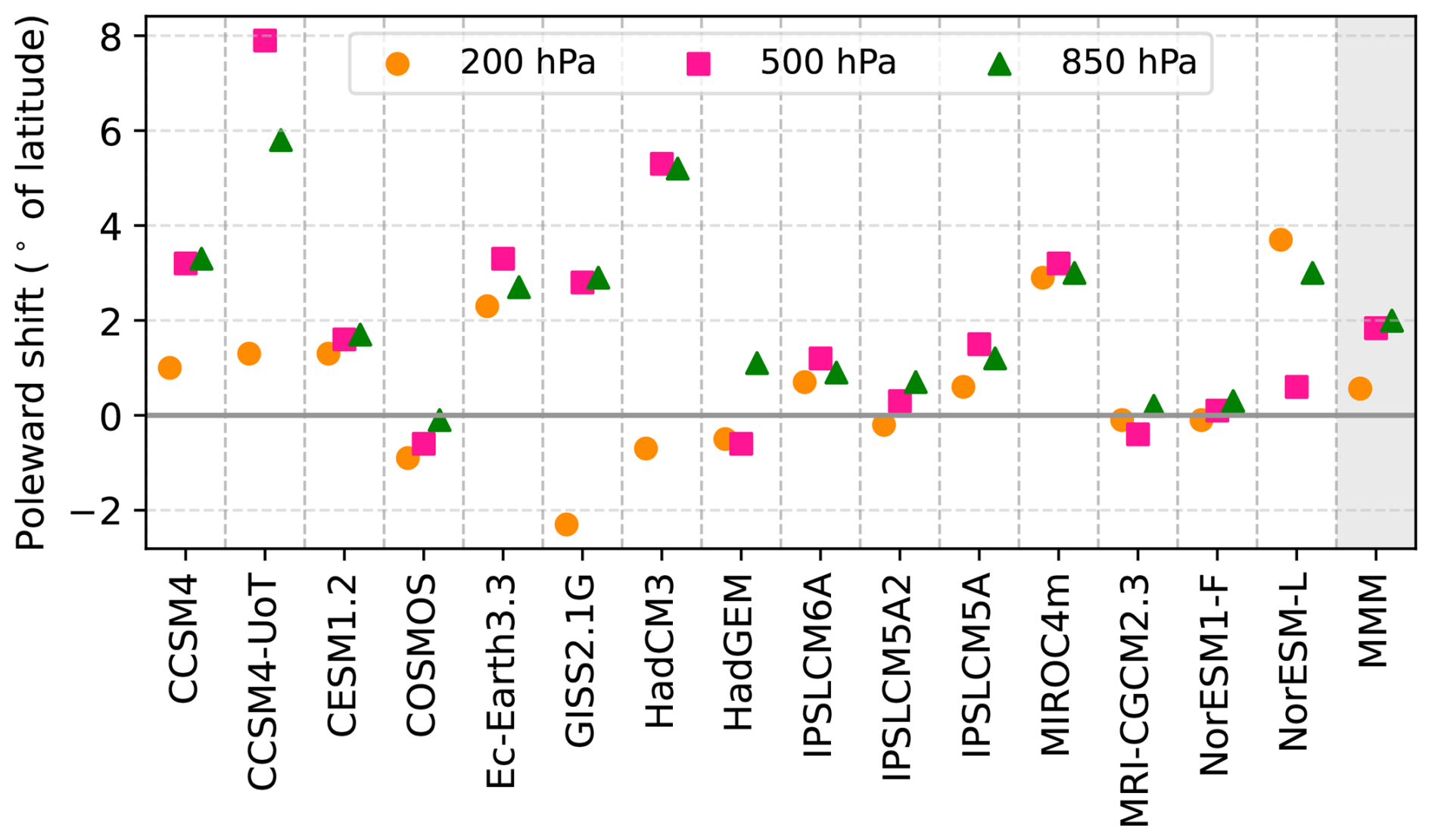
Figure 2 Poleward shift of the latitude of maximum zonal wind in the North Pacific region in boreal winter (DJF) at three pressure levels across all the models and the multi-model mean (MMM). Positive values indicated the jet is poleward in the Late Pliocene experiments compared to the pre-industrial control simulations.

In the North Atlantic region, a double peak in the zonal wind speeds can be seen, likely due to the presence of Rossby wave breaking (Fig. 1d), which can also be seen in Fig. 3. None of the models, with the exception of HadGEM3, capture the reanalysis well at this level (Fig. S3), with the MMM zoanl wind speed being higher than the reanalysis. This is expected as models often underperform in the North Atlantic region (Anstey et al., 2013). When considering the MMM change, a poleward shift and a slight strengthening in the winds are observed. After removing the data points at 200 hPa from CCSM4-UoT and CESM1.2 (due to large shifts in the maximum from increased wave breaking), the North Atlantic jet stream shifts by 1.9, 0.4 and 1.1° at 200, 500 and 850 hPa respectively. There is also lower model spread with only two models exhibiting a large equatorward shift. The MMM, however, is driven by some models with larger changes, such as HadCM3 and MRI-CGCM2.3 (Fig. S3).

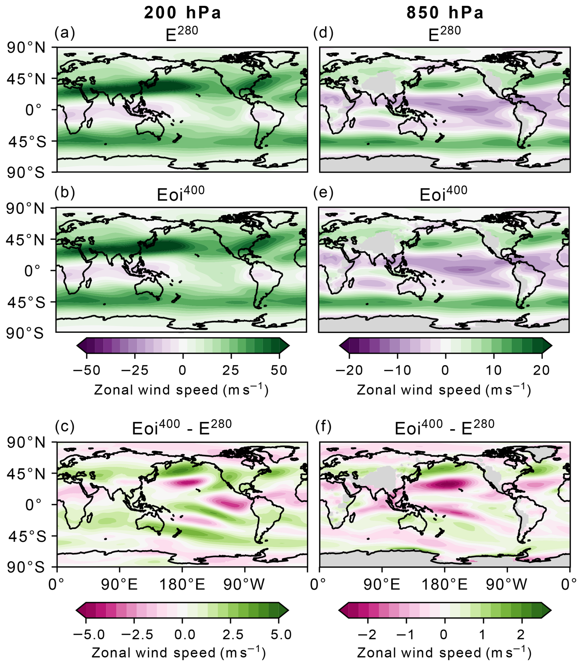
Figure 3 Multi-model mean zonal wind speeds for 200 hPa (a–c) and 850 hPa (d–f). The lower plots show the difference between the Late Pliocene (Eoi⁴⁰⁰) and the Pre-Industrial (E²⁸⁰). Note the difference in scales between the two pressure levels.

Considering the spatial variations, the change is seen as a strengthening on the poleward flank and a weakening at the equatorward flank at both the 200 and 850 hPa level (Fig. 3). The MMM difference in Fig. 3 is muted compared to the differences seen when examining the individual model differences. This may be due to differences in the placement of the jet stream and the magnitude of poleward shift cancelling in the MMM (Figs. S4 and S5).

In the North Pacific, the weaker and poleward shifted westerly winds at 850 hPa are consistent with proxy data. Abell et al. (2021) examine changes in the strength and position of the jet stream using dust flux records in the warmer Pliocene climate compared to cooler glacial climates. They report that in warmer climates, like the Late Pliocene, the westerly winds are poleward and weaker compared to cooler climates matching what is found in this modelling study. More work is needed to fully assess the dust flux records in different ocean basins to understand the full proxy signal. However, it is difficult to obtain data at a high enough temporal resolution to support this analysis. It is also possible that changes in dust flux and aerosols may lead to changes in atmospheric circulation if there is a change in land surface type although Abell et al. (2021) argue that atmospheric circulation is the dominant driving factor of the observed flux changes.

There are several reasons for differences between models. First is the resolution of the model. Models with grater spatial resolution are able to capture more complex ocean–atmosphere interactions that play a large role in the representation of atmospheric circulation (Athanasiadis et al., 2022). Models with finer spatial resolution will also include a better representation of orographic features affecting both ocean and atmospheric circulation. Some models are obvious outliers from the reanalysis data, such as IPSLCM5A, IPSLCM5A2, COSMOS, HadCM3 and NorESM-L (Figs. S2 and S3). These are the models among the lowest spatial resolution of PlioMIP2 (Table 2). This indicates that model resolution is an important factor to consider when examining changes in the jet stream. There is also added uncertainty in the representation of the jet stream within the ERA5 reanalysis, as observations higher in the atmosphere are sparse. Some models also better capture proxy reconstructions of sea surface temperatures, for example, CCSM4-UoT, CESM1.2, IPSLCM6A and MIROCm4m (Haywood et al., 2020). These models may also be able to provide a better representation of jet stream changes during the Pliocene as they capture the general climate of the Pliocene well.

To examine possible causes of the change to the mean state jet, the change in jet stream latitude is compared to the ratio of the earth system sensitivity (ESS) and the equilibrium climate sensitivity (ECS) to assess the relative contribution of CO₂ and non-CO₂ forcings. However, no strong or significant relationship was detected (Fig. S6) suggesting that drivers of the change in the jet may not be consistent across the range of models. To fully understand the drivers of jet stream change, each model will need to be individually examined.

3.2 Controls on the mean state shift using HadCM3

To understand which of the Pliocene boundary conditions contribute to the change in the mean state jet stream we use the HadCM3 forcing factorisation experiments described in Sect. 2.1.2. HadCM3 displays a small (0.7°) equator ward displaced jet in DJF at 200 hPa, but it does show poleward movement of 5.3° and 5.2° at 500 and 850 hPa respectively, and a weaker jet. Although considering MMMs is important, there is limited data to perform full forcing decomposition with the full range of the PlioMIP2 models. It should also be noted that it is impossible to fully disentangle the contribution of ice sheets and orography because the two are inherently interlinked per the boundary condition design in PlioMIP2. The ice sheet itself provides a change in orography, which is especially important for controlling changes in the North Atlantic jet stream with the position of Greenland being important for the pattern of the jet stream in that region (White et al., 2019).

The HadCM3 DJF surface temperature forcing decomposition can be seen in Fig. S7. This highlights the regional influences of changes to temperature from ice sheets and orography with the largest changes occurring where the changes to ice sheets and land sea mask were made. The Late Pliocene experiment has a stronger AMOC compared to the pre-industrial simulation, consistent with other models in the PlioMIP2 ensemble (Zhang et al., 2021; Weiffenbach et al., 2023). The experiments employing Late Pliocene orography (including land–sea mask changes) show a stronger AMOC than the experiments with pre-industrial orography (Fig. S8). This is likely due to changes in the Northern Hemisphere ocean gateways. This is consistent with previous studies, which relate the increase in Late Pliocene AMOC to the closure of the Arctic Ocean gateways (Otto-Bliesner et al., 2017; Weiffenbach et al., 2023). This enhanced AMOC, due to ocean gateway changes, is one contributor to the reduced meridional temperature gradient, as more heat is transported northward. In the forcing factorisation experiments, vegetation changes are included in the orography boundary condition. A change in vegetation can also lead to a large change in temperature, due to different plant types having different impacts on temperature through albedo and evapotranspiration (Bonfils et al., 2012). Studies examining other time periods have reported that changes in vegetation in response to climate reinforce the signal, especially at high latitudes (O'ishi and Abe-Ouchi, 2013; O'ishi et al., 2021).

Figure 4 shows the total change in zonal wind speed between the pre-industrial and the Late Pliocene simulations in HadCM3 and the contribution of CO₂, ice sheets and orography. In the North Pacific, the change in wind speed due to CO₂ is small (and opposite in sign to the other forcings), with the largest contribution being orography (including land–sea mask and vegetation) and ice sheets following as the second leading cause in the change. Following the discussion about AMOC and vegetation impacts, this change could be due to changes to meridional temperature gradients. Over the North Atlantic, changes to the ice sheets have a larger effect, which is expected due to changes in the Greenland Ice sheet.

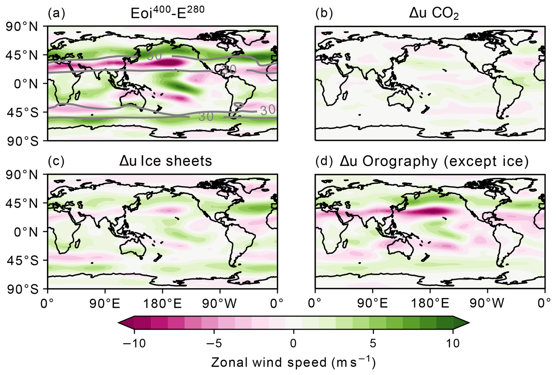
Figure 4 Change in boreal winter (DJF) 200 hPa zonal wind speed between the Late Pliocene (Eoi⁴⁰⁰) and the Pre-industrial (E²⁸⁰) in HadCM3 and the contribution of the change from CO₂, ice sheet and orography forcing to the total change. In plot (a) the grey contours show the 30 m s⁻¹ value in the E²⁸⁰ experiment.

The leading contribution from orography is also apparent when considering the North Pacific vertical profile of the zonal wind speeds (Fig. 5). The contributions from CO₂ and ice sheets are also small here. Examining the change in the North Pacific vertical profiles of temperature (Fig. 6a), the decreased meridional surface temperature gradient is seen and is attributed to a change in the CO₂. Orography contributes to warming in the mid-latitudes troposphere and cooling aloft in the high latitudes. This pattern of warming may be contributing to changes in the geopotential height (Fig. S9) with CO₂ increasing the height globally. However, ice sheet and orography changes produce strong spatial variation, especially over the Allusion low region, consistent with previous studies (Menemenlis et al., 2021; Oldeman et al., 2024). It is unclear what is causing this warming over the North Pacific region. There is a pattern of warming from orography in the surface temperature (Fig. S7), although it is not known if this is due to a change in ocean circulation or a response to the changes in atmospheric circulation. It is also acknowledged that the North Pacific jet stream is impacted by other areas of the world, including changes in the Tropics (Oldeman et al., 2024).

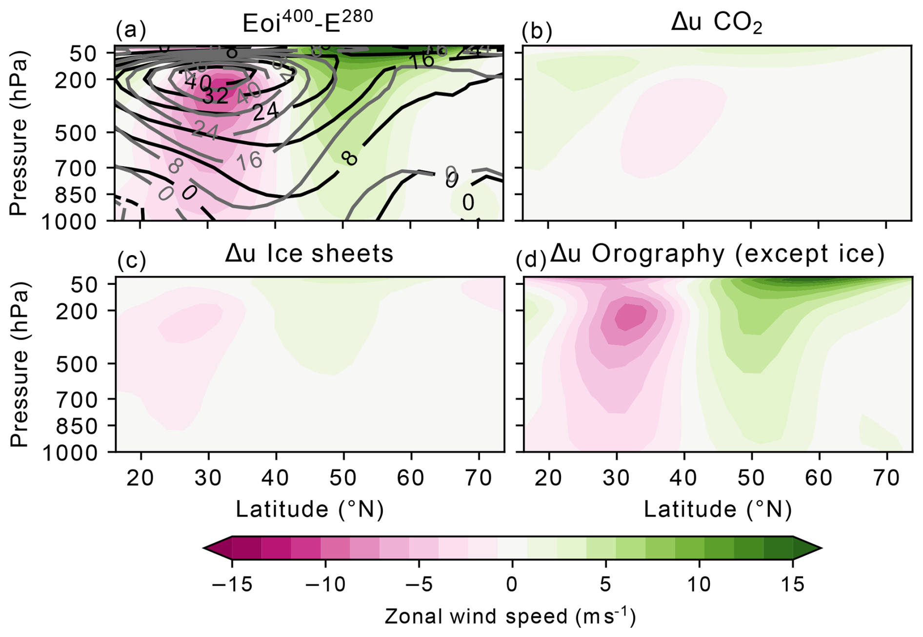
Figure 5 Change in boreal winter (DJF), zonally averaged, North Pacific zonal wind speed between the Late Pliocene (Eoi⁴⁰⁰) and the Pre-industrial (E²⁸⁰) in HadCM3 and the contribution of the change from CO₂, ice sheet and orography forcings to the total change. In plot (a) the grey contours represent the E²⁸⁰ values and the black contours represent the Eoi⁴⁰⁰ values.

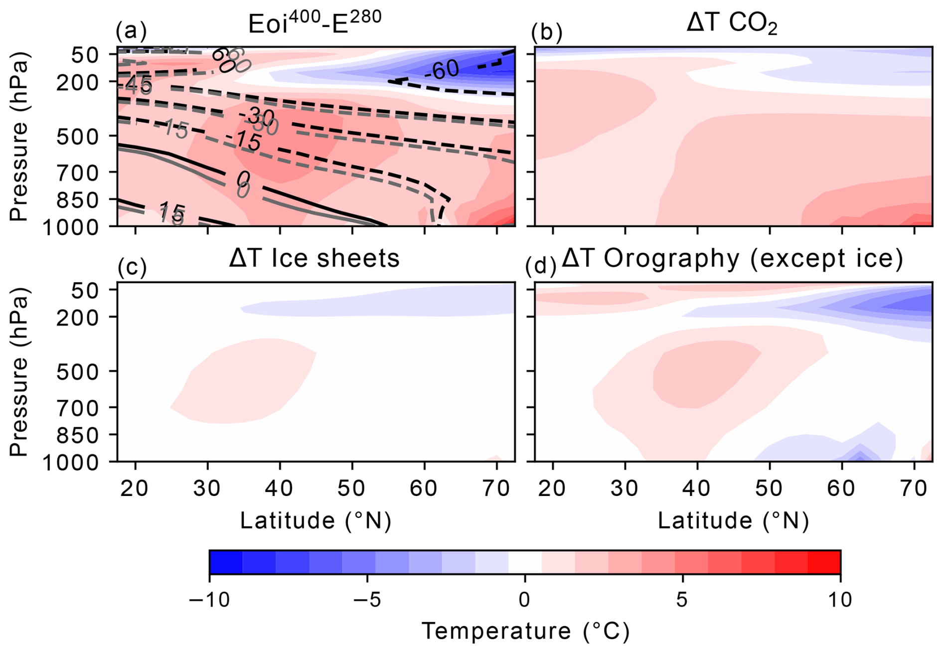
Figure 6 Change in boreal winter (DJF), zonally averaged, North Pacific temperature profile between the Late Pliocene (Eoi⁴⁰⁰) and the Pre-industrial (E²⁸⁰) in HadCM3 and the contribution of the change from CO₂, ice sheet and orography forcings to the total change. In plot (a), the grey contours represent the E²⁸⁰ values and the black contours represent the Eoi⁴⁰⁰ values, and dashed lines indicate negative values.

Two other models, CCSM4-UoT and COSMOS also provide the simulations needed for a full forcing factorisation. The results of the vertical profiles of the North Pacific zonal wind speeds are found in Figs. S10 and S11. In COSMOS (Fig. S10), each boundary condition change contributes small amounts to the total change and in CCSM4-UoT the orography contribution is similar to HadCM3, but also contains a pattern from the ice sheets resembling the orography pattern. The main differences in the setup of these experiments between models are the implementation of different land sea masks. COSMOS uses the standard boundary conditions (Stepanek et al., 2020), and CCSM4-UoT uses the enhanced boundary conditions but retains a Late Pliocene land sea mask in the Ei experiment. This suggested the change in the wind due to orography is driven by changes to the land sea mask used. To fully understand this an analysis of ocean circulation in each model and experiment would be needed, but is beyond the scope of this study.

3.3 Jet stream variability in the North Pacific

Although jet stream variability has been investigated in similar manner before within CCSM4-Utrecht only (Oldeman et al., 2024), as discussed in Sect. 3.2, there are large differences in the mean state shift across the ensemble. This range in responses for the mean state may also suggest differences in simulated variability across the ensemble, highlighting the importance to examine variability in a multi-model setting. To assess the model performance against ERA5 reanalysis data we compare the mean latitude and variability in position in the pre-industrial simulations over the North Pacific against reanalysis data (Fig. 7). The majority of models capture the jet latitude variability but there is a larger spread in the mean jet latitude. Models that are furtherest away from the reanalysis tend to have lower spatial resolutions (COSMOS, MRI-CGCM2.3 and MIROC4 m). The impact of multi-decadal variability cannot be ignored in this assessment and some longer modes of variability may be influencing the 100 year mean.

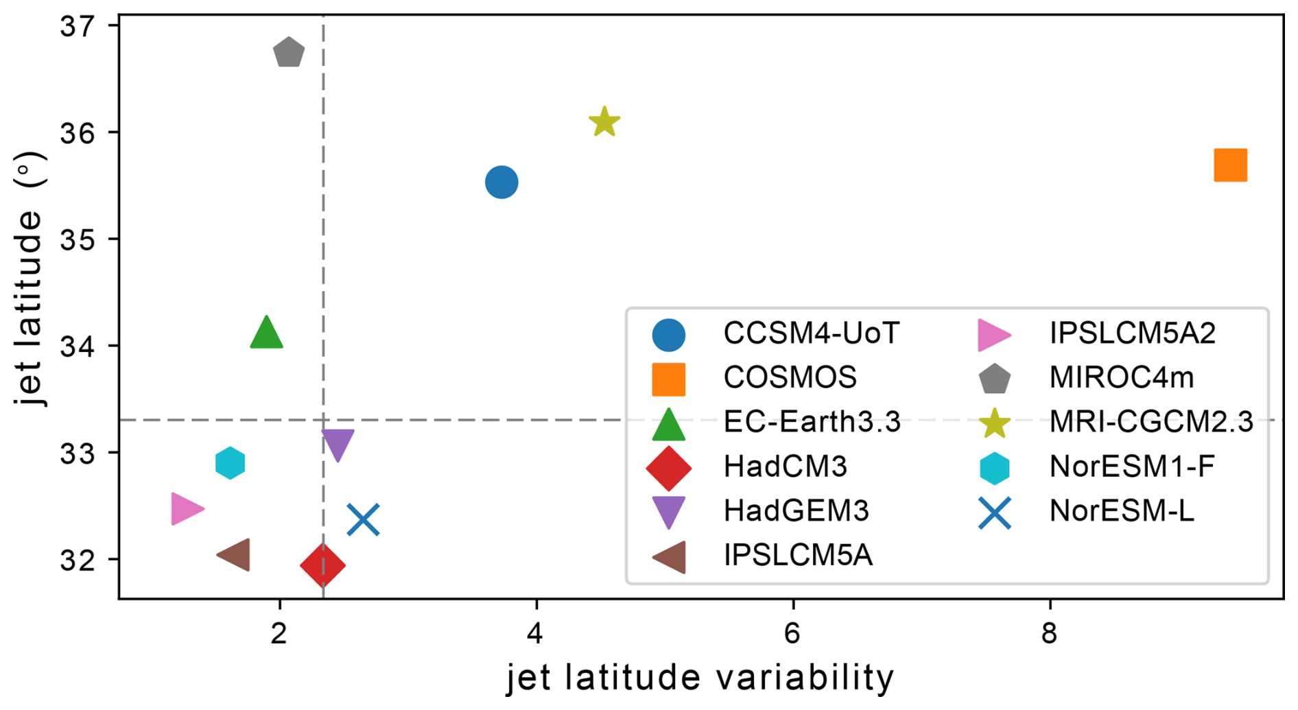
Figure 7 Latitude of maximum zonal wind speed and standard deviation of this latitude (jet latitude variability) in the PlioMIP2 E²⁸⁰ (pre-industrial) simulations compared to the ERA5 reanalysis data (dashed grey lines) in the North Pacific region for January.

The response to Late Pliocene boundary conditions across models is diverse (Fig. 8). The difference between models is larger than the difference caused by a change from pre-industrial to Late Pliocene boundary conditions, indicating that care should be taken in the interpretation of these results as the model uncertainty is large. However, some models may be better at capturing the change in the jet stream variability than others. For example, HadGEM3 and MRI-CGCM2.4 have an unchanged land–sea mask. Since we expect the differences observed in the jet to be partially caused by land–sea mask changes, we do not expect a large change in the jet stream in these models, as is seen in Fig. 8. The impact of model resolution is also clear from Fig. 8 with the lower resolution models displaying a more diffuse maximum (COMSOS, MRI-CGCM2.3 and NorEMS-L).

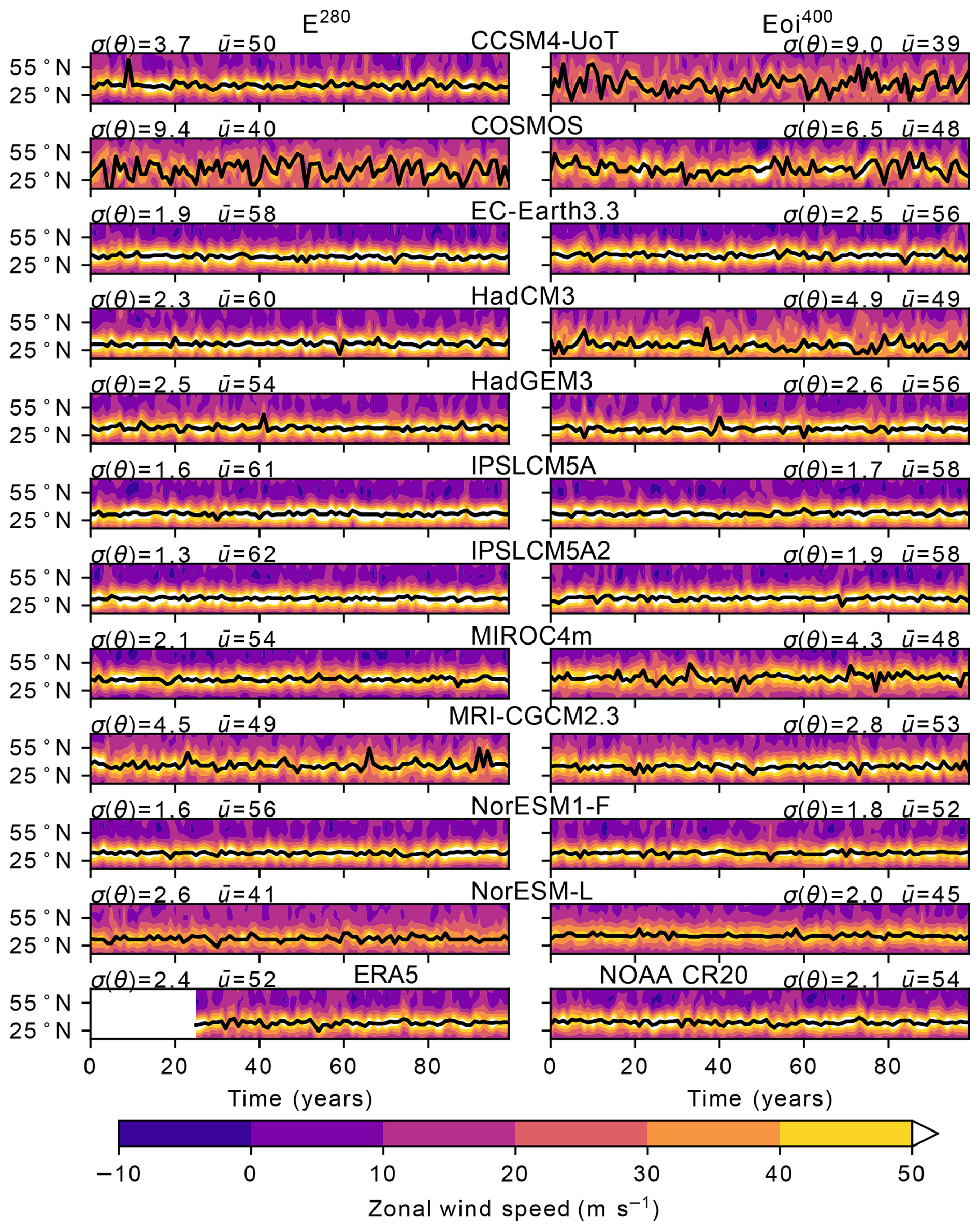
Figure 8 Hovmöller diagrams for the zonal mean wind speed at 200 hPa in January for 100 years for the North Pacific. The left-hand side is from the E²⁸⁰ (pre-industrial) experiments and the right-hand side is from the Eoi⁴⁰⁰ (Late Pliocene) experiments with the exception of the bottom two panels which show the reanalysis data. The black line indicates the latitude of maximum zonal wind speed. The standard deviation in the latitude (σ(θ)) and mean maximum zonal wind speed ($\stackrel{\mathrm{‾}}{u}$) are shown for each subplot.

The jet stream latitude variability (σ(θ) in Fig. 8) is higher in the Late Pliocene than in pre-industrial experiments in most models. However, a lot of this change is only small (Fig. 9). HadCM3, CCSM4-UoT and MIROC4 m all show a larger change in the variability of the jet stream. Two models that show an increased speed and a decreased variability, COSMOS and NorESM-L, are the two models with the lowest resolution out of the PlioMIP2 ensemble. This reinforces that resolution does matter when considering jet stream dynamics. MRI-CGCM2.3 also shows an increase in speed and a decrease in variability which could be related to the unchanged land–sea mask in the Late Pliocene experiment in this model. The models with a Late Pliocene land–sea mask and higher spatial resolution indicate that the jet stream is weaker and more variable in the Late Pliocene. The change in the variability of the latitudinal position of the jet stream could be related to increased wave breaking in the Late Pliocene (Oldeman et al., 2024).

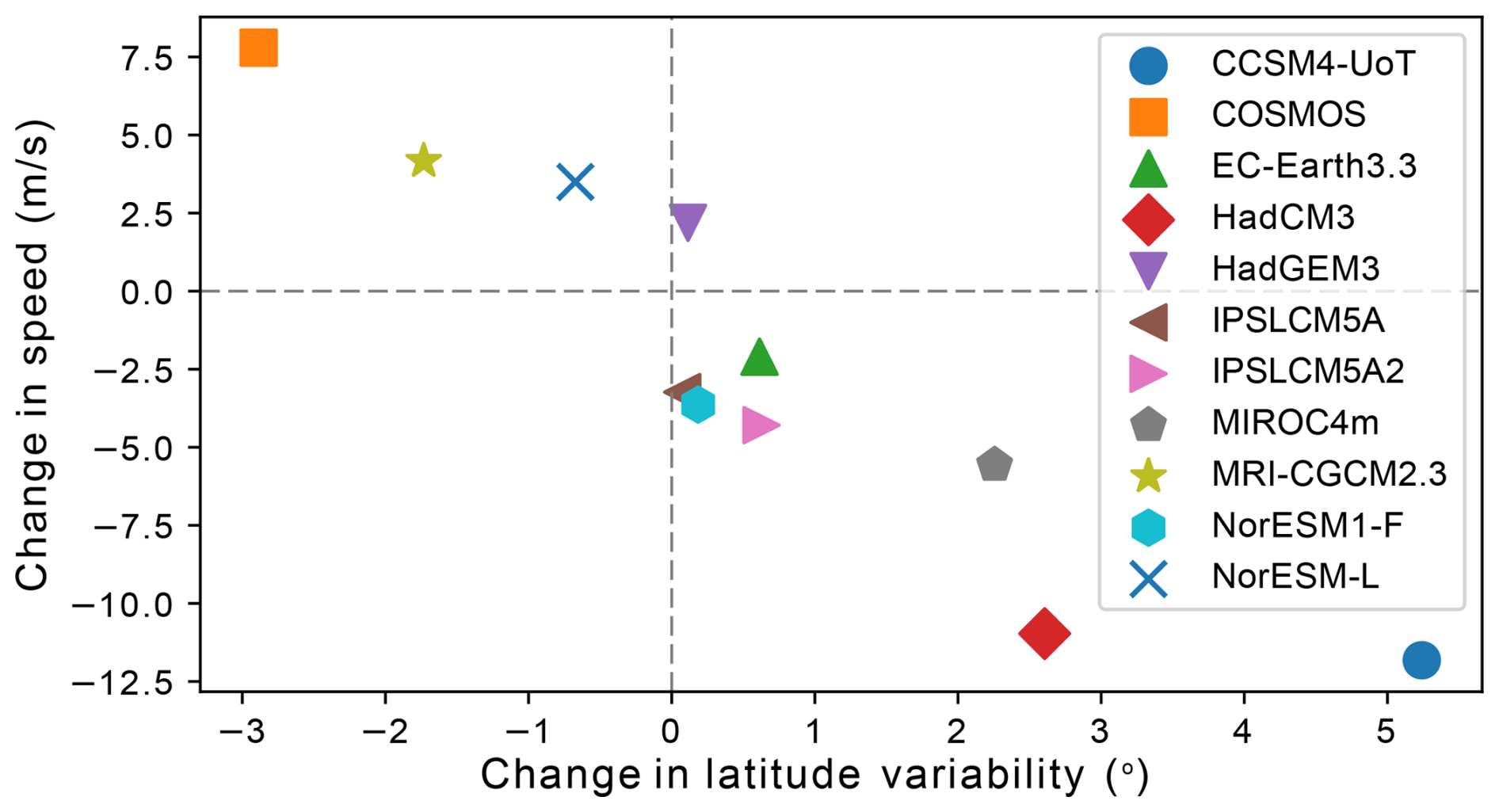
Figure 9 Change in the mean speed of the January North Pacific jet stream and the change in the variability of the jet stream position. Each model in the ensemble is labelled. The dashed grey lines divide the graph into quadrants, where the upper left section shows models with an increased speed and decreased variability and the lower right quadrant contains models with a slower speed and increased variability.

3.3.1 Forcing decomposition of jet stream variability

In HadCM3, the North Pacific Late Pliocene simulation jet stream is weaker and more variable in position than in the pre-industrial simulation (Fig. 9) in agreement with the majority (7 of 11) of the models. Using the new forcing factorisation experiments the contribution of each boundary condition change can be assessed to understand if the drivers of the mean state also drive changes to the variability. Figure 10 shows the jet stream variability (σ(θ)) in each of the 8 simulations. There is little contribution of CO₂ to the total change, evidenced by experiments with the same ice sheets and orography, but a change in CO₂ having no large change in speed or variability. The largest change in interannual variability comes from the alterations to the orography boundary conditions. This relates to the change in the mean state with the orography having the largest impact on the zonal wind speeds (Figs. 4 and 6). As the largest changes in variability are due to non-CO₂ boundary conditions, this suggests the Late Pliocene is not an analogue for future, CO₂ driven, jet stream variability.

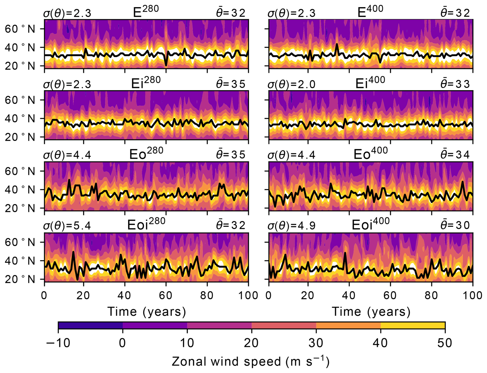
Figure 10 Hovmöller diagrams for the zonal mean wind speed at 200 hPa for 100 Januaries for the North Pacific from the eight HadCM3 experiments. The black line indicates the latitude of maximum zonal wind speed. The mean latitude of the jet ($\stackrel{\mathrm{‾}}{\mathit{\theta }}$), and the standard deviation in the latitude (σ(θ)) are shown for each experiment.

As declining sea ice has been shown to have links with changes in mid-latitude winter time circulation (Smith et al., 2022), the relationship between sea ice area and some jet stream metrics has been included here. Figure 11 shows a clear grouping of the experiments using Late Pliocene orography vs. experiments with pre-industrial orography. This grouping in the sea ice could be explained by either a stronger AMOC or a reduction in Arctic sea surface area due to the implementation of Late Pliocene boundary conditions (or a combination of both). Sea ice area reinforces Arctic amplification, with a reduction in sea ice cover lowering albedo, which in turn warms the Arctic (Jenkins and Dai, 2021). This Arctic amplification, leading to a weakening in the meridional temperature gradient, could create a slower jet stream (Francis and Vavrus, 2015; Smith et al., 2022).

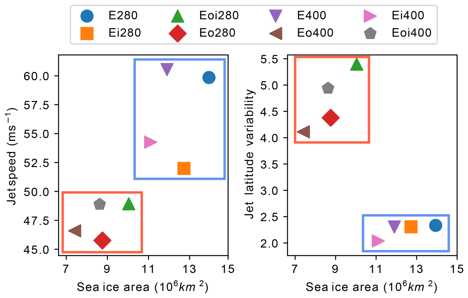
Figure 11 January Northern Hemisphere sea ice area and January North Pacific jet stream speed (left), and jet latitude variability (right) at 200 hPa in HadCM3. The red box groups experiments with Late Pliocene orography and the blue box groups experiments with pre-industrial orography.

The CCSM4-UoT and COSMOS models also provided forcing factorisation experiments. The variability in the jet stream across the 8 simulations for these models can be found in Figs. S12 and S13. The COSMOS model differs from the other two models with the forcing fractionation experiments as the jet stream was stronger and less variable in the Late Pliocene simulation. However, it is unclear from the forcing factorisation what causes this (Fig. S12). There is little change between all of the experiments with the exception of a strengthening in the full Late Pliocene experiment, potentially a feature of a lower resolution model and consistent with the zonal wind changes in Fig. S10. In CCSM4-UoT CO₂ has little impact on the speed and variability of the jet, but both orography and ice sheets contribute to the slowdown and increased variability observed in the Late Pliocene experiment (Fig. 13). This equal contribution from ice sheets and orography was also noted in previous studies that examined upper troposphere dynamics (Menemenlis et al., 2021) and again is consistent with the vertical profile of zonal wind speeds (Fig. S11). Sea ice extent was also examined in CCSM4-UoT (Fig. S14). Here, a larger contribution from ice sheet changes to variability and speed is also seen. In CCSM4-UoT, there is no significant difference in the AMOC amongst the forcing factorisation boundary experiments (Chandan and Peltier, 2018), meaning that northward heat transport may not be different between the runs. This could explain why the jet CCSM4-UoT is more sensitive to ice sheet changes than HadCM3. Part of this could be due to the boundary conditions being slightly different in each model, with the land sea mask around Antarctica being treated differently in each model which may create some of the differences observed in the AMOC. The model dependency of this jet stream latitude variability change highlights the need for climate variability to be studied from a multi-model perspective, especially in a palaeoclimate setting where there is often only one realisation of each experimental setup, limiting the ability to assess internal variability of climate models.

4 Conclusions and future directions

By examining models within the PlioMIP2 ensemble, it is found that during the Late Pliocene, the jet stream was weaker and exhibited a poleward shift in the North Pacific region compared to the pre-industrial control period. The effect varies between models due to a number of factors including the extent of land sea mask modification and potentially model resolution. Examining higher frequency variability shows that the jet stream may be more variable in the Late Pliocene, although again this is model dependent. However, the models with the largest reduction in jet stream speed also show the largest increase in variability. From new experiments using HadCM3, it is found that a change in the orography, including land–sea mask and vegetation, is the leading cause of the change in the jet stream. This could also explain why models that do not change the land–sea mask do not see a weaker or more variable jet in the Late Pliocene.

As we approach a warmer, unknown future, studies have invoked the Pliocene as an analogue for future climate given the similarity of global mean Pliocene temperatures to projections for the end of this century (Burke et al., 2018; Burton et al., 2023). As the majority of the difference in the jet stream variability is caused by changes to orography, this element of the Late Pliocene climate system is not relevant to future change. Although the mechanism of change (a change in upper level temperature gradient) may be similar to modern climate (Woollings et al., 2023), as the direct causes of this are different, comparisons need to be made with care. Impacts of the reduced ice sheets may be relevant for longer time scales as a reduction in the ice sheet size occurs, but as the climate is a complex system with many interactions and feedbacks, it may not be possible to apply this result directly to future projections. This agrees with previous studies on jet stream variability, which state that the Late Pliocene is not an analogue for future Northern Hemisphere winter time variability (Oldeman et al., 2024).

This work could however have impacts on the study of the Late Pliocene climate. As the jet stream becomes weaker and more variable, more persistent weather patterns may occur leading to a change in the frequency and intensity of extreme events. A change in the distribution of key climate variables (such as temperature and precipitation) could impact the way that model comparison with proxy data is interpreted. As higher frequency temporal variability is lost when performing proxy analysis, a change in variability between the reference period and the time period in question could change the way that the climate signal is transferred into a proxy variable, e.g. temperature. Further work is needed to fully understand how this change in the jet stream relates to surface changes, for example, by studying how the jet stream interacts with different modes of climate variability (for example, the North Atlantic Oscillation and the Pacific Decadal Oscillation).

This paper shows the importance of considering climate variability, and the drivers of it, for studies of the Late Pliocene, particularly when thinking of it as an analogue for future climate. As there is a range of responses across models, this work also highlights the need for multi-model comparisons for assessing a change in internal variability.