Information loss in palaeoecological data from process and observer error

Palaeoecological data provide insight into how ecosystems have changed in the past, and, with the development of new sources of proxy data and statistical methods, they are being used to address questions around the underlying mechanisms of change, such as biotic- and climate-ecosystem interactions. However, inferences from palaeoecological data can be hindered by uncertainties inherent in core-type samples that arise from environmental processes and observer-introduced error. Environmental processes, core extraction methods, sub-sampling strategies, laboratory methods, and data processing can potentially mask “true” signals in the data. How different sources of uncertainty influence the inferences drawn from palaeoecological data is rarely assessed, but is critical to the confidence of our conclusions. To address this concern, we use a virtual ecological approach to assess the effects of environmental and observer introduced uncertainty to better understand which of them most influence statistical methods applied to the data. Quantifying information loss from uncertainty can inform study design before a project is carried out, and so increase the likelihood of detecting a given signal of interest and make more robust inferences from statistical analyses of palaeoproxy data. We generate synthetic “error-free” core-type samples of pseudoproxies, on which environmental and observational processes are systematically introduced to impose uncertainties on the simulated pseudoproxies. The influence of three sources of uncertainty (core mixing, sub-sampling, and proxy quantification from sub-subsamples), are assessed for their individual and combined effects on two statistical methods used to synthesise palaeoecological records: Fisher Information and principal curves. Increasing sub-sampling intervals has the most influence on the two statistical methods applied to the pseudoproxy data. When combined, the interaction between increasing sub-sampling interval, and decreasing the number of proxies counted per sub-sample has the strongest influence on Fisher Information and principal curves. Fisher Information and principal curves are not affected in the same way by introducing uncertainty, with principal curves being less influenced by simulated proxy counting and sub-sampling of the core. Virtually assessing uncertainties is a powerful method to better understand the influence that uncertainties introduced at different parts of the analytical process have on conclusions drawn from palaeoecological data.

1 Introduction

Palaeoecological data extends the temporal extent over which we can investigate ecosystem change well beyond the observational record (Kosnik and Kowalewski, 2016). These long-term records are crucial for understanding ecosystem trajectories and climate-ecosystem interactions, as such dynamics may unfold over centuries or millennia (Jackson, 2007). Many proxies and statistical methods are used to address how ecosystems respond to environmental and human pressures through time. Palaeoecologists use these data to go beyond describing past changes in, for example, the relative abundances of species, to uncover underlying mechanisms of change such as biotic interactions and species-environment relationships (Williams et al., 2011). However, the inferences drawn from palaeoecological data may be limited by their uncertainties, such as a paucity of observations over time and space, environmental degradation of samples, and observer-introduced error. Thus, to make robust inferences from palaeoecological data, such uncertainties need to be better understood and quantified. Here, we focus on proxies reflecting species community data such as fossil pollen extracted from a core sample and quantified on microscope slides.

1.1 Uncertainties in palaeoecological data

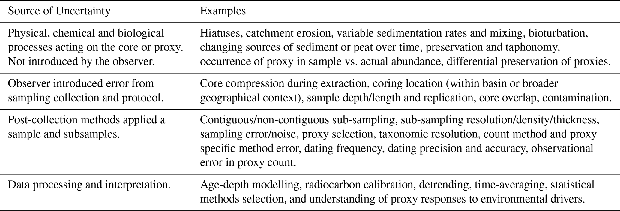
Palaeoecological data derived from core-type samples are subject to numerous uncertainties, including: (i) environmental effects and landscape processes affecting the sample before extraction; (ii) the methods used in the field to extract the sample; (iii) laboratory techniques applied to extract and quantify data from the core; and (iv) quantitative analyses applied to the data (Table 1). Environmental processes and observation error can affect the representation of species in the data (e.g., their observed relative abundances; Goring et al., 2013). Sub-sampling strategies may alter the chronological placement of events (Liu et al., 2012; Parnell et al., 2008). Manipulation of data, such as interpolation to satisfy statistical assumptions, can introduce statistical artifacts and increase type-I error rates (i.e., a false positive). Such uncertainties affect the robustness of statistical results and the inferences we may draw from them.

Table 1 Sources of uncertainty from pre-sampling natural processes to statistical analyses of data. Uncertainties are not independent across categories and can propagate through the observational process and subsequent analyses.

1.2 Pseudoproxy experiments and virtual ecology

Virtual ecology (VE) can be used to assess the influence of uncertainty on statistical methods and associated inferences (Zurell et al., 2010). In the VE approach, simulated data are used as testbeds for recreating, in simulation, observational processes. The synthetic data provide an “error-free” benchmark against which to assess simulated observational processes and analytical methods. The underlying concept is that the synthetic data mimic the statistical properties of empirical data without being subject to the same issues of, for example, limited grain size or extent (Smerdon, 2012). Similarly, the simulated observational process aims to recreate the statistical properties of the observer, such as the chance of observing a species occurring at low abundances. Here, we adopt a VE approach to (i) assess uncertainties introduced by environmental processes and observer-introduced error by simulating data analogous to a sediment core-type sample, and (ii) to virtually recreate environmental processes acting on a core, and the observational methods used to extract data from the core sample. The VE approach follows the form: generate data → simulate the observational process → analyse the “true” and “observed” data → assess the analyses of the observed data against the “true” data. We extend this approach to include simulated environmental process errors that occur before the observational process. The steps of our adapted VE approach: data generation, degradation, observation, analysis, and assessment are described in Sect. 2.1 through 2.3. Empirical data typically lack an “error-free” control, and even high-quality empirical data (e.g., highly resolved proxy data from a laminated lake sediment core) incorporate multiple uncontrollable sources of uncertainty. Virtual experimentation allows for the effects of sources of uncertainty to be explored for their individual and interaction effects in a systematic and controlled way (Smerdon, 2012).

The VE approach is similar to pseudoproxy experiments where modified observational data or pseudoproxies (i.e., simulated proxy data) are used in place of empirical observations (Mann and Rutherford, 2002) and analysed in the same way as empirical measurements (Asena et al., 2024). Pseudoproxy experiments originated in climatology where they are a method of assessing palaeoclimate reconstructions (Bothe et al., 2019; Christiansen et al., 2009; Mann and Rutherford, 2002); here, we apply the same concepts to palaeoecological data. We use the term virtual ecology to describe the approach by which synthetic data are generated, sampled from and analysed in ways comparable to empirical data (Zurell et al., 2010). While simulated data cannot substitute entirely for reality, they provide an experimental platform (sensu Peck, 2004) with which to understand the processes that influence the formation and analysis of empirical data.

Pseudoproxies have been widely used in climatology (Bothe et al., 2019; Mann and Rutherford, 2002), but virtually assessing sampling methods and statistical approaches on palaeoecologically relevant data is less common (although see Asena et al., 2024; Benito et al., 2020; Blaauw et al., 2010). The lack of understanding of how uncertainties in palaeoecological data affect the inferences made from them has raised concern (Blaauw, 2012; Blaauw et al., 2020). We address this knowledge gap by:

• i.

  generating multivariate pseudoproxy archives (considered analogous to a time series of proxy data from a core sample);

• ii.

  introducing environmental uncertainty to the pseudoproxy archives via simulated core mixing;

• iii.

  introducing process and observer error by virtually recreating the observational processes of sub-sampling the core and quantifying proxies from the sub-samples; and

• iv.

  applying two multivariate statistical methods independently, Fisher Information (FI; Fisher, 1922) and principal curves (PrC; Hastie and Stuetzle, 1989), to analyse the “error-free” and degraded/sub-sampled data.

• v.

  feature analysis methods (a dimensional-reduction method that collapses time-series to a set of metrics) are then applied to the FI and PrCs to quantify the effect of increasing levels of uncertainty

Our overarching aim is to quantify the information loss in palaeoecological analyses from environmental uncertainties, and process and observer error, and how this influences statistical analysis and inference using such data. We use FI and PrCs as examples that capture the underlying drivers of a system in different ways. FI captures shorter-term variance e.g., those driven by short-term stochastic processes. PrCs, as a method of indirect gradient analysis, primarily captures the long-term ecosystem trends in the pseudoproxies resulting from the primary driver in the scenarios. A better understanding of how individual and combined sources of uncertainty affect statistical results and interpretation can help inform study design (e.g., determining the number of replicate cores or the sub-sampling resolution needed to detect a signal of interest) and the confidence in the statistical results of a study.

2 Methods

2.1 Simulating pseudoproxies

Pseudoproxies are simulated using the model described in Asena et al. (2024), following the proxy system model (PSM) framework (Evans et al., 2013) where a sensor (e.g., terrestrial vegetation) responds to environmental drivers and records that response via proxies (e.g., fossil pollen) counted in an archive such as a lake sediment (in this case a pseudoproxy record). The model we use follows the conceptual framework of a PSM, but is not process-based. We adapt the PSM conceptual framework (Evans et al., 2013) to explicitly include degradation models that describe archive-altering processes before observations are drawn (Fig. 1). Asena et al. (2024) describe the three sub-models that generate the pseudoproxy data: (i) a driver model representing the environment in which the archive forms; (ii) a sensor model representing the response of a sensor (e.g., terrestrial vegetation) to the environment; and (iii) an archive model that represents how the response of the sensor is recorded (e.g., as fossil pollen) in a medium such as a sediment core.

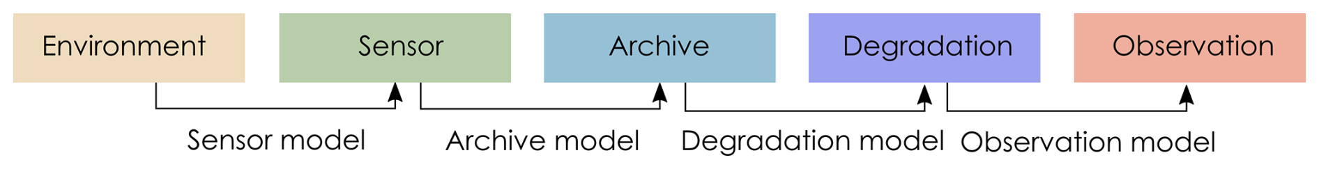
Figure 1 Adapted Proxy System Model framework (Evans et al., 2013) describing the process by which environmental drivers act on a sensor, which records its response in an archive, from which observations are drawn. We have included degradation models to describe processes acting on the archive before observations are drawn.

“Error-free” pseudo proxies are simulated – in the environment, sensor, and archive sub-models (Fig. 1). The model consists of four components: (i) environmental driver change over time (environment); (ii) species' niches with respect to the driving environment (the sensor response); (iii) pseudoproxy abundances recording the response to driver change in an archive (archive record); and (iv) a representation of the formation of the core (archive characteristics such as core length and accumulation rate). In summary, the model generates archives of pseudoproxies consisting of 200 potential species representing a palaeoecological record free from the process and observer error associated with empirical data. Pseudoproxy abundances are a response to extrinsic and dynamic environmental drivers with intrinsic variability from disturbance events, introduction to the population via dispersal, and variation in carrying capacity over time. Each species has a tolerance for each environmental driver that, together, defines the species niche and determines the population growth rate of a species at any given time-step as a function of the environmental drivers. If any of the environmental drivers fall outside of a species tolerance to that driver, the species will have a negative growth rate and may eventually become locally extinct. Species that are tolerant of the current environmental conditions can be introduced via dispersal, thus creating a species turnover as conditions change. Simulating 200 species covers a wide range of the driver parameter space and allows different species assemblages to emerge as driver conditions change. Only a subset of the 200 species will be presented in the simulated community at any one point in time.

Thirty-one replicate models were run for a duration of 5000 time-steps with a burn-in period of 500 time-steps applied to allow species to stabilise with respect to the driving environment. We aimed for a minimum of 30 replicates to account for model variance, and 5000 time-steps (ca. 5000 years) was sufficiently long to represent ecological turnover in the model The scenario we present here has two environmental drivers: (i) an abrupt environmental driver switching between constant conditions; and (ii) a random walk driver weighted to 0.15 of the total environmental effect. The magnitude of change in the abrupt driver is insufficient to cause a complete species turnover, and generalist species survive the shift in extrinsic conditions. The random walk driver may amplify or dampen the effects of the abrupt driver, but in general is favourable to most species in the system. The parameters for each species are randomised for each replicate model run around the same baseline parameters (Table S2 in the Supplement). The results of an additional three scenarios with different environmental drivers can be found in the Supplement. We present the abrupt change scenario for two reasons: (i) there are empirical examples of such events (e.g., the termination of the Younger Dryas and the Bølling–Allerød warming; Williams et al., 2011), and (ii) an abrupt shift in community composition is more likely to be detected by statistical analyses. If the statistical methods we assess perform poorly on the abrupt scenario, they are unlikely to perform better on more gradual community turnover.

Each simulated core is characterised by simulated age, considered to be one year per time-step, and an increase in depth per time-step. The accumulation rate is represented by a combination of a linear decrease with time, with a smoothed random walk superimposed to represent core compression in addition to landscape variability. Variable sedimentation rates result in a different core length (and accumulation per time-step) for each replicate simulation and change the number of model time-steps included in a sub-sample of one-centimetre thickness. Variable change in depth per time-step is calculated as a smoothed and scaled random walk (similar to Benito et al., 2020) representing landscape changes and possible hiatuses. A gradual decrease in depth with age can occur from compaction or compression during extraction (Taranu et al., 2018). The simulated data represent a core-type sample from which sub-samples are taken, proxies quantified, and data analysed similar to real-world core samples. The simulated core is used as an “error-free” benchmark against which methodological and statistical processes are assessed and represents the complete (and un-degraded) absolute abundance of proxy data.

2.2 Degradation and sampling of pseudoproxies

In this section, we describe the degradation model representing post-depositional processes affecting the pseudoproxy data (in this case, core mixing), and the observation models (Fig. 1) representing how proxies are quantified from a core sample (here, sub-sampling and the count method applied to micro-fossils on microscope slides). For details and visualisations of the degradation models, see Asena et al. (2024). We apply three treatments to each of the model replicates: mixing (degradation), sub-sampling and proxy counting (observation), applied at 10 levels each individually and combined (Fig. 2). Together, the degradation and observation models represent process- and observer-introduced error that affect the data before quantitative analyses are applied. Each of the 31 replicate archives results in 1210 datasets from the “error-free” reference core to the most uncertain.

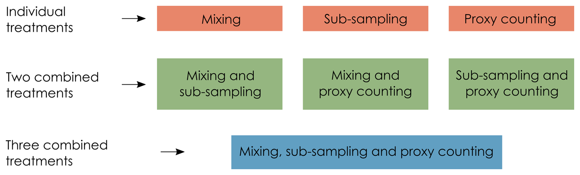
Figure 2 Each uncertainty (treatment) is applied to the “error-free” pseudoproxy archive to systematically introduce uncertainty individually, and in combination.

2.2.1 Virtual mixing: degradation model

Core mixing is applied as a centrally weighted rolling-average over time-windows of the archive ranging from unmixed (the “error-free” benchmark) to a window of 10 time-steps. Simulated mixing is represented as consistent over time, rather than being a depth-dependent process such as bioturbation.

2.2.2 Virtual sub-sampling: observation model

An absolute proxy abundance per time-step is generated by the model and is sub-sampled at regular depth intervals ranging from one to ten centimetres. Each sub-sample has a thickness of one centimetre; the number of time-steps spanned by the sampled thickness is determined by the simulated accumulation rate. If the one-centimetre sub-sample covers multiple time-steps, the proxy abundances in that sub-sample are summed. All sub-sample treatment data are converted to relative abundances before analysis so that the analyses are not influenced by excessive values from the summed proxies of multiple time-steps. When applied in combination with simulated proxy counting, values are converted to relative abundance after the proxy count treatment.

2.2.3 Virtual proxy count: observation model

The process of counting proxies in a sub-sample (e.g., counting several hundred pollen grains or diatoms on a microscope slide) is simulated by random sampling from the absolute proxy abundances with resolutions increasing from 100 to 1000 by 100. The probability of a proxy occurring in the random sample is based on the abundance of that proxy. The sample is then converted to relative abundances comparable to empirical proxy data. The simulated count treatment is applied to the raw, mixed, and sub-sampled data. Increasing levels of uncertainty in the proxy counting treatment are represented by a decrease in the proxy count resolution.

2.3 Quantitative analyses

After the application of the degradation and observation models, the pseudoproxy data span a gradient of uncertainty from the “error-free” data to the uncertain data that reflect what we observe from a system. We then apply statistical analyses along this gradient to determine the influence of each source of uncertainty (the penultimate step of the VE approach). FI and PrCs are used to analyse each treatment level from each replicate core (treatment level being the severity of each of the treatments, mixing, sub-sampling and proxy counting). FI and ordination methods have been suggested as appropriate where there are an unlimited number of input variables of any data type that do not require a priori knowledge of the driving state variables of a system (Roberts et al., 2018). The FI and PrC produce a large amount of data, so we use feature analysis for time-series (FATs; Nun et al., 2015) to synthesise them and reduce each time-series to a small number of metrics (or “features”) that we can compare across treatment levels (detailed below). Each replicate core results in 1210 FI time-series and PrCs, and by extracting a set of features, the difference among treatment levels can be calculated as a measure of distance, we use Euclidean distance. The data analysis process is as follows: (i) calculate FI and PrC for each treatment level; (ii) extract features from the FI and PrC outputs; and (iii) calculate the distance between the features of each treatment level (Fig. 3).

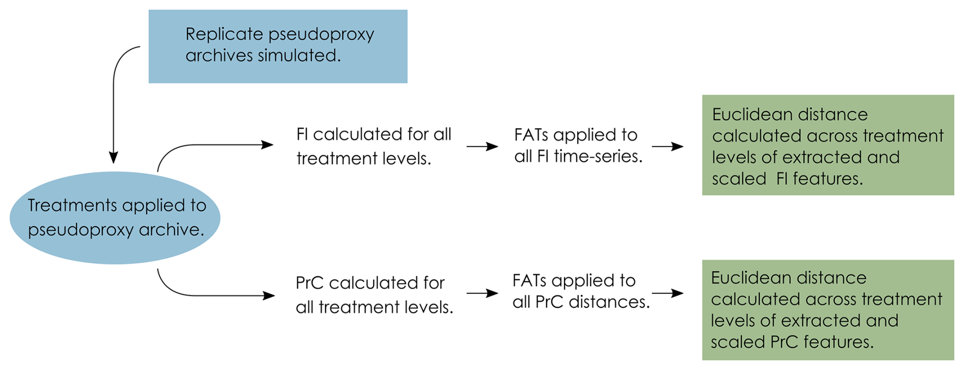
Figure 3 Conceptual data-flow of the degradation, sampling and analysis process. Treatments of mixing, sub-sampling and proxy counting are applied individually and in combination to the replicate pseudoproxy archives (Fig. 2). Fisher information (FI) and principal curves (PrC) are applied separately to each treatment and subsequently analysed using feature analysis for time-series (FATs). Extracted features are scaled and Euclidean distance between each treatment level and the “error-free” reference core is calculated.

2.3.1 Fisher Information (FI)

Fisher information was developed to quantify information about an unknown parameter from measurable variables (Fisher, 1922) and has since been used as a measure of ecosystem stability (Cabezas and Fath, 2002; Eason et al., 2016; Karunanithi et al., 2008; Mayer et al., 2006). Fisher information has been applied to palaeoecological data, with the suggestion that it can be used as an indicator of an approaching regime shift, such as a shift in diatom species' composition (Spanbauer et al., 2014). Fundamentally, FI evaluates the probability of detecting different system states over time, or the “stability” of the system; thus, FI changes with the variance in the system. Pseudoproxies from each replicate core, and each level of uncertainty, are analysed using FI, using a custom R package (Asena et al., 2023).

2.3.2 Principal curves

Principal curves can be used to identify the underlying variables (e.g., a steadily changing variable over time) that describe a system characterised by multiple state variables and can be considered as a form of non-linear principal components analysis (De'ath, 1999). In short, a PrC is a one-dimensional curve fit through the “middle” of an n-dimensional space (e.g., species composition data; (Hastie and Stuetzle, 1989). The curve represents species compositions by mapping (or projecting) the sites, e.g., the species' composition at a given sample, onto a low-dimensional space, and using similarity or dissimilarity measures to measure the distance between sites (assessing, for example, the species' compositional change through time). The arrangement of sites reflects the composition of species in the reduced dimension space as the distance between sites is proportional to the distance in species composition (De'ath, 1999). Principal curves can be used as a method of gradient analysis, the underlying concept being that the species abundances change in a predictable way along an ecological gradient. Here, we use PrCs to represent change in species composition over time and as a method of indirect gradient analysis using the distances along the PrC. Cubic smoothing splines are used to fit the PrC to the data. Hastie and Stuetzle (1989), De'ath (1999), and Simpson (2012) detail the implementation of PrCs. PrC analyses were conducted for all replicate pseudoproxy datasets for each level of increasing uncertainty using the analogue package (Simpson and Oksanen, 2020) in R (R Core Team, 2020).

2.4 Assessing results: Feature analysis for time-series

The final step of the VE approach is to assess the outcomes of the statistical analyses applied to the degraded and sampled data against the “error-free” pseudoproxies. To compare the FI and PrC time-series across treatment levels, we use feature analysis. Feature analysis is a method of reducing a two-dimensional time-series to a one-dimensional set of “features”. Features are metrics that describe a time-series in terms of summary statistics (e.g., mean and variance), and more complicated descriptors such as autocorrelation length (Nun et al., 2015). We developed a set of 62 features (Table S4) drawing on feature analysis for time-series (Kim et al., 2011; Nun et al., 2015; Richards et al., 2011; Sokolovsky et al., 2017) and change point analysis (Killick and Eckley, 2014). The individual and combined degradation and sampling treatments result in 1210 time-series per replicate, yielding 31 × 1210 = 37 510 virtual cores per scenario. Describing the FI time-series and PrC as a series of features allows comparison between the 1210 treatments by calculating a distance measure (we use Euclidean distance) between the extracted features of each treatment level. The feature analysis process is as follows:

1. Features are extracted from the FI time-series and distances along the PrCs for all replicate model runs of the “error-free” archive.

2. A correlation matrix of the features from the replicate “error-free” datasets is constructed, and features with a Pearson's correlation coefficient greater than $\left|\mathrm{0.7}\right|$ are excluded sequentially, recalculating the correlation matrix until all highly correlated features are dropped, starting with the highest correlation coefficient (Dormann et al., 2007).

3. The remaining features (with a Pearson's correlation coefficient less than $\left|\mathrm{0.7}\right|$) are then calculated for all replicates across all treatment levels, resulting in a number (ranging between 14–26 per scenario) of single metric features per treatment that describe the FI time-series and PrC.

4. The features are scaled (by subtracting the mean of the entire series from each point and dividing it by the series' standard deviation), and the Euclidean distance is calculated across treatment levels, resulting in a single distance measure between the “error-free” core and each treatment level.

5. Summaries of the Euclidean distances are calculated for all treatment levels across replicates, resulting in a single distance measure for each treatment from the “error-free” benchmark.

3 Results

3.1 Effects of individual sources of uncertainty

In the extracted features for FI, sub-sampling causes the largest overall increase in the median Euclidean distance from the “error-free” core, followed by proxy counting and then mixing; however, there is overlap in the confidence envelopes across all three treatments (Fig. 4A). Distance from the “error-free” core increases consistently with uncertainty in the mixing treatment, showing a steeper increase in distance across uncertainty compared with the other two treatments. Between successive treatment levels, proxy counting shows little increase in the median Euclidean distance as uncertainty increases. In the sub-sampling treatment, distance increases more in the lower uncertainty levels than in the higher levels, plateauing somewhat at higher uncertainty (Fig. 4A). There is some variability across the treatment levels resulting from the stochasticity in the underlying model and simulated observational processes (i.e., proxy counting is a random sampling process, and sub-sampling is dependent on the variable accumulation rates of the core).

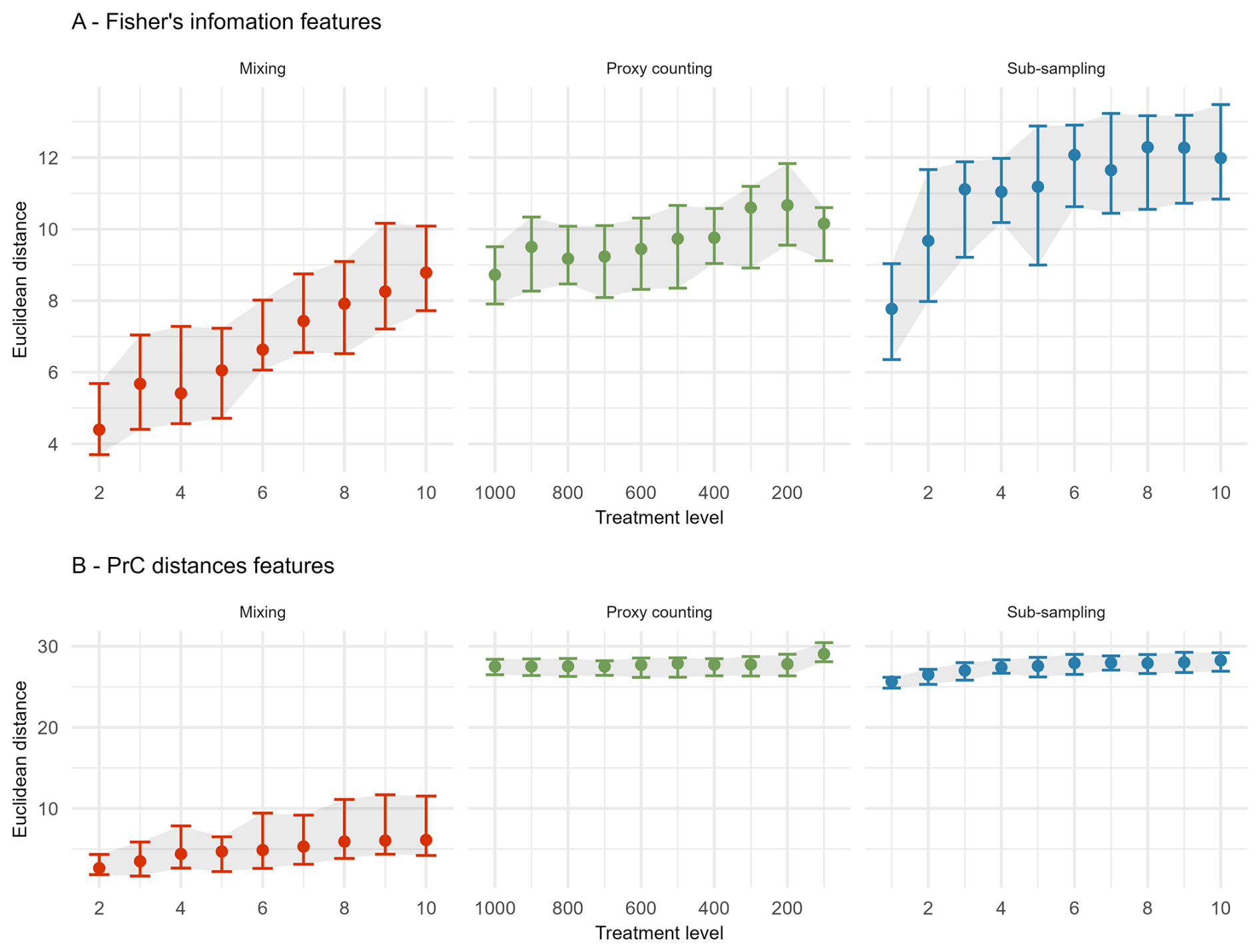
Figure 4 The median (dots), 25th, and 75th quantiles (error-bars and shaded area) of the Euclidean distance from the “error-free” core of features extracted from the Fisher information (A) and PrC distances (B) calculated across replicate simulations. Note the x-axis is organised so uncertainty consistently increases from left-to-right.

For the PrC features, across all scenarios the mixing treatment has the least effect on median Euclidean distance (Fig. 4B). Proxy counting and sub-sampling have overlapping confidence envelopes, although they are much smaller than those of the mixing treatment. Proxy counting shows no consistent pattern in median Euclidean distance between successive treatment levels until the lowest count resolution. Conversely, the sub-sampling treatment shows an increase in the lower treatment levels, plateauing as sub-sampling interval increases (Fig. 4B).

3.2 Effects of two combined sources of uncertainty

In the following section, treatments are applied simultaneously to determine which combinations cause the greatest effect on analyses of the core. The greatest increase in mean Euclidean distance on the features extracted from FI from the “error-free” core arises from the interaction of the sub-sampling and proxy counting uncertainties increasing together (i.e., along the diagonal; Fig. 5A), with a stronger effect from the subsampling treatment. Mixing combined with sub-sampling or with proxy counting shows no clear interaction effect as the treatments increase in severity together. The smallest increase in distance is from the combination of mixing with proxy counting, suggesting that sub-sampling tends to have the greatest influence of the three treatments (Fig. 5A). The effect of the mixing treatment on the mean Euclidean distance is small when compared to those of either sub-sampling or proxy counting (Fig. 5A). Variability across the surface of each plot emerges from underlying model stochasticity, random sampling in the simulated count method, and the variable accumulation rates of the replicate cores.

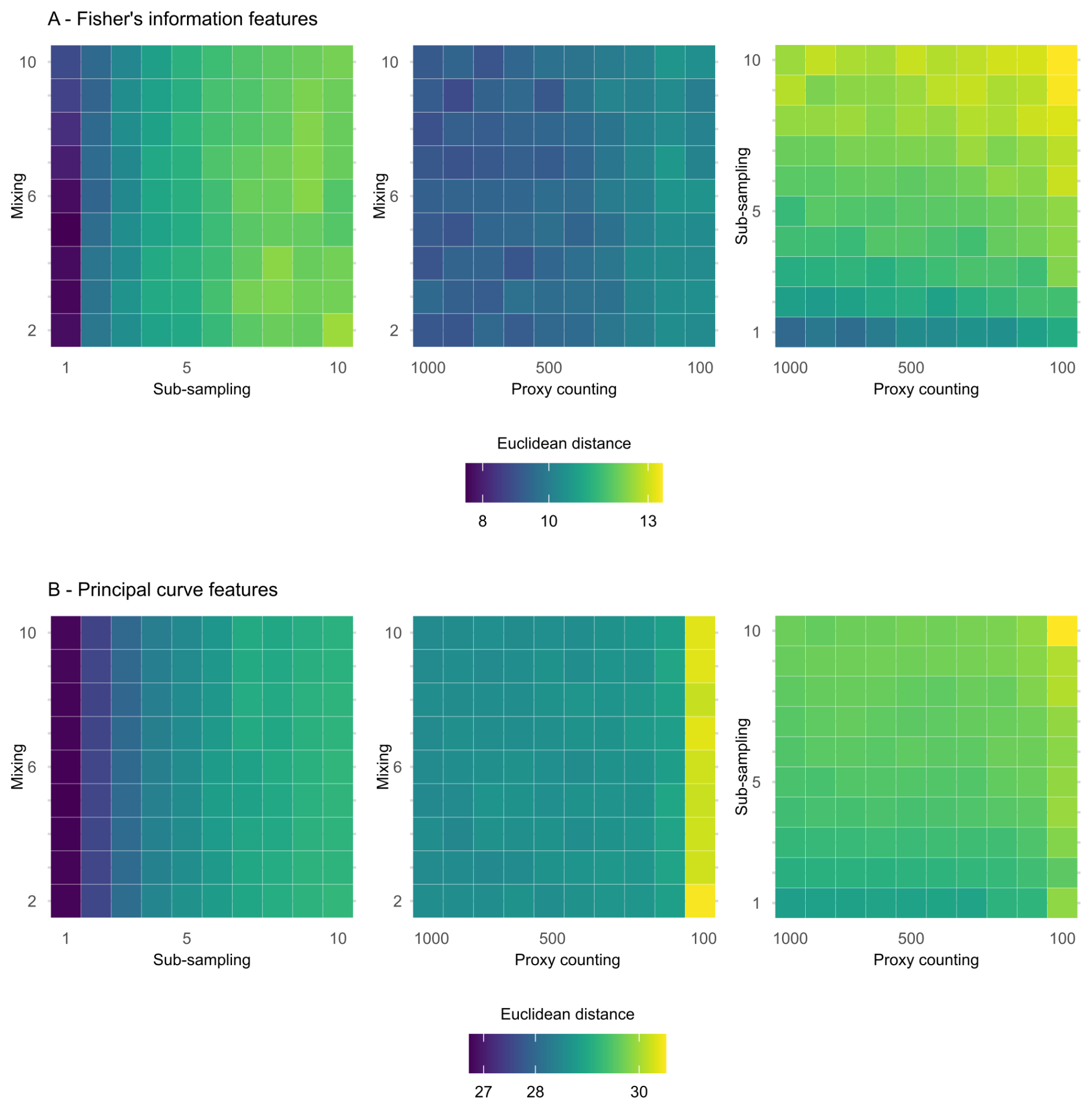
Figure 5 Mean Euclidean distance of features from the “error-free” core of two treatments combined calculated across replicate simulations for Fisher information (A) and principal curves (B). The mixing axis shows the number of time-steps over which mixing occurs. Along the sub-sampling axis, the frequency of sub-sampling in centimetres is shown, and the proxy counting axis displays count resolutions in number of individuals counted per sample. In the proxy counting treatment, uncertainty increases as count resolution decreases.

In the extracted features from the distances along the PrCs, the combined effects of sub-sampling with proxy counting show the largest increase in the mean Euclidean distance of all the combined treatments, with a weak interaction effect as proxy count and sub-sampling uncertainties increase together (Fig. 5B). No interaction effect is visible in either the combined treatments of mixing with sub-sampling or mixing with proxy counting (Fig. 5B).

3.3 Effects of three combined sources of uncertainty

Interaction effects of all three uncertainties applied simultaneously were assessed for the extracted FI and PrC features (Fig. 6). An interaction effect is visible in the increase of mean Euclidean distance as the sub-sampling interval increases (along the x-axis), together with proxy counting resolution decreasing (across facets from top left to bottom right); however, no clear increase is visible along the mixing axis, indicating little contribution from mixing to the interaction of the three treatments (Fig. 6). Overall, the greatest increase in the mean Euclidean distance among treatments is at the lowest proxy count and largest sub-sampling interval.

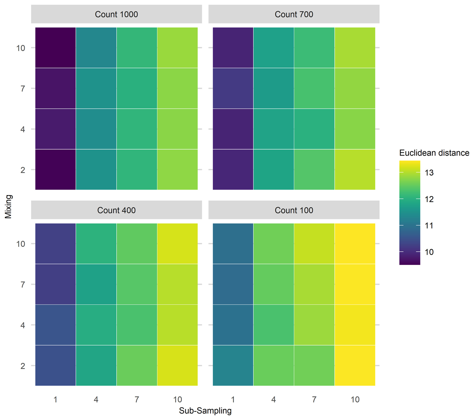
Figure 6 Mean Euclidean distance of Fisher's Information from the “error-free” core for three treatments applied in combination. To demonstrate the three treatment dimensions, results are displayed such that each plot axis shows mixing (number of time-steps over which mixing occurs) and sub-sampling (frequency in centimetres) treatments, and each facet (sub-plot) is the proxy counting treatment (number of individuals counted in sub-sample). Uncertainty from proxy counting increases from the top left to the bottom right.

In the PrC features, applying three treatments in combination does not show a clear three-way interaction as uncertainty increases (Fig. 7). An increase in mean Euclidean distance is visible along the sub-sampling axis (as sub-sampling interval increases), but there is little visible effect of the proxy counting treatment (reducing in resolution across facets from top left to bottom right) until the lowest resolution. Mixing contributes relatively little to the overall increase in mean Euclidean distance showing no visible increase along the mixing axis (Fig. 7).

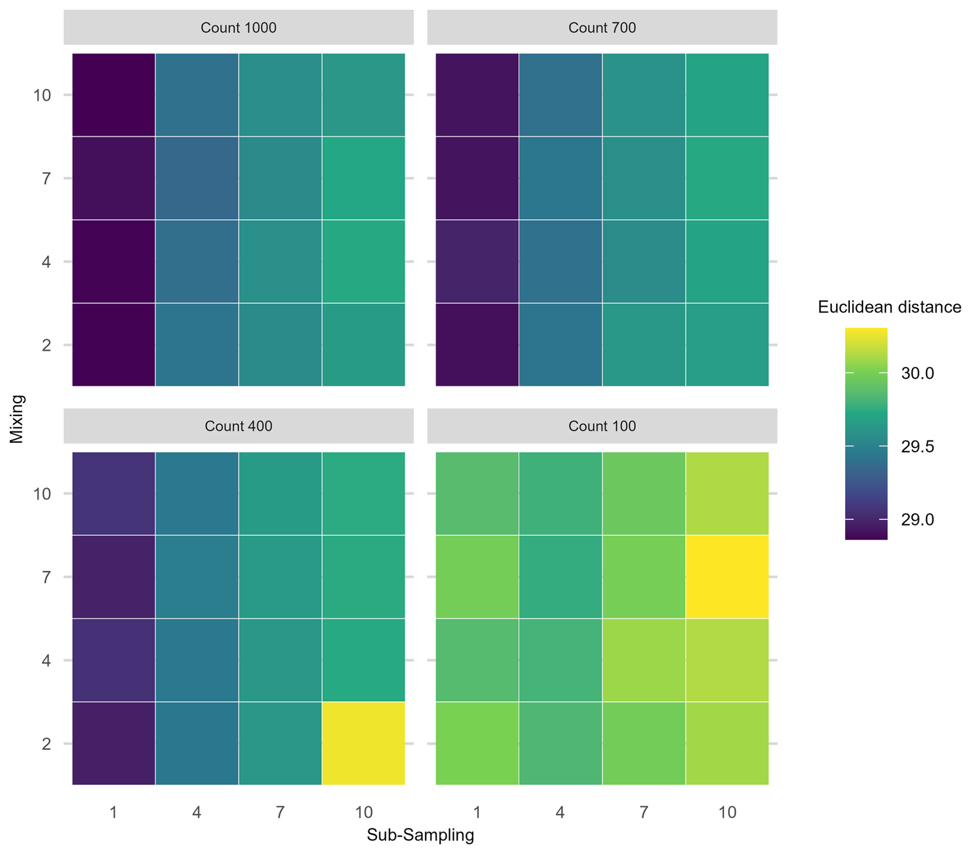
Figure 7 Mean Euclidean distance of the principal curves from the “error-free” core of all uncertainties increasing in combination. Same plot layout and interpretation as Fig. 6.

4 Discussion

To draw reliable conclusions from palaeoecological data, it is crucial to view our inferences in the context of the uncertainties they integrate. Our goal in this paper was to address how process and observer error affect statistical methods applied to palaeoecological data and the inferences we draw from them. Here, we have assessed some of the uncertainties that affect species proxy data. Additionally, uncertainty arises from building chronologies (Blaauw et al., 2018; Parnell et al., 2008; Telford et al., 2004) and measuring abiotic system variables, such as isotopic records and lake level reconstructions, which carry their own uncertainties.

4.1 Effects of individual sources of uncertainty

Without exception, sub-sampling treatments show the largest effect on the median Euclidean distances of the FI features (with some overlap in the confidence envelope with the proxy counting treatment), followed by the proxy counting process. For the PrC features, both sub-sampling and proxy counting treatments had a similar effect on Euclidean distance. For both the FI and PrC features, the smallest effect on Euclidean distance between the “error-free” and degraded cores came from the simulated mixing degradation process.

Perhaps the most interesting implication of our analyses in the context of empirical ecology is how the effects of sources of error differ between the two statistical metrics (FI and PrC). Beyond the initial increase in Euclidean distance in the PrC from the application of proxy counting and sub-sampling (an unavoidable cost), there was little further effect until the lowest proxy count and sub-sampling resolutions. Thus, PrCs may be a useful measure of a system's trajectory for patchy data (e.g., initial analysis of low sub-sampling resolution data before deciding where to focus sampling effort). For FI, treatment effects have a more consistent increase in distance from the “error-free” core with treatment intensity. The short-term variability captured by FI may provide useful system indicators (sensu Eason and Cabezas, 2012) but may also require high-quality data (e.g., high sub-sampling resolution and proxy counting) for reliable inferences. The required temporal resolution of the data is also likely to increase if accumulation rates are slow and species turnover is rapid. Increased sub-sampling frequency is required in systems that change rapidly compared with more stable systems where the difference between successive time-steps is small. Slow accumulation rates mean that a one-centimetre-thick sub-sample integrates multiple years of ecological change; thus, uncertainty from sub-sampling resolution will increase if the accumulation rate is slow and ecological change is rapid. An observer may interpret FI results with the knowledge of which sources of uncertainty, whether controllable (e.g., sub-sampling and proxy counting resolution) or uncontrollable (e.g., mixing and accumulation rates), have the greatest influence. After introducing uncertainties to the pseudoproxies, the primary patterns, such as long periods of increase in FI, remain visible and offer a useful depiction of community change.

4.2 Effects of combined sources of uncertainty

For both FI and PrC, when two treatments are applied in combination, the greatest overall increase in mean Euclidean distance from the “error-free” core resulted from sub-sampling uncertainty in combination with proxy counting uncertainty. For the PrC the maximum increase in mean Euclidean distance for two simultaneous treatments occurred at the lowest proxy count resolution in combination with mixing, but such a low proxy count resolution is unlikely in any empirical study. In our analyses, mixing has relatively little effect compared with sub-sampling or proxy counting, and the effect tends to be obscured by other sources of stochasticity (disturbance, dispersal, and temporal changes in carrying capacity), variable accumulation rates, and randomised sampling of the proxy abundances. Similarly, when three sources of uncertainty are combined, mixing shows the least effect, and no apparent interaction with sub-sampling or proxy counting. However, it is worth noting, that our implementation of mixing is relatively simple in that the effect on the pseudoproxy data is a centrally weighted smoothing. More extreme mixing, and time-varied mixing effects are likely to show a stronger effect.

In the case of FI, the greatest benefit in terms of reducing the distance from the “error-free” core came from increasing sub-sampling resolution followed by proxy count resolution. However, from the standpoint of an observer, increasing the resolution of an FI time-series may not increase the information content, at least in terms of capturing long-term patterns. Simple driving environments (e.g., the single driver simulations) are likely to be adequately represented by FI applied to low-resolution data; however, interpretation of FI from environments influenced by multiple drivers is potentially challenging without considerable knowledge of the underlying driving conditions. The benefit of the VE approach is that it allows us to examine how the underlying dynamics manifest in multivariate indicators of change, such as FI; however, such near-complete information is rarely, if ever, available. Ultimately, an observer must base sampling and analysis decisions on their specific aims. If accurate evaluation of short-term variability is a goal (e.g., for studies of ecosystem resilience), then dedicating resources to sub-sampling resolution is likely to be beneficial to analyses such as FI. Reducing observer error, a more controllable source of error, may help detect a short-term signal of interest if the uncontrollable sources of error, such as sediment accumulation rates, mixing, and driver variability, are sufficiently small that the signal remains detectable.

PrC shows little increase in distance (after the initial increase from the application of the treatments) from the “error-free” reference with combined treatment levels. Thus, as a representation of compositional change, it may be robust to low-resolution data (e.g., infrequent sub-sampling). Short-term changes in abundance (e.g., small disturbances) will likely become less evident in the PrC; however, our results suggest that overall patterns seen in a PrC are robust to multiple sources of error. Thus, from the perspective of an observer, high-resolution data may only be required for PrC to identify short-term compositional changes, such as perturbations that take a few generations to recover from.

4.3 Lessons from virtual ecology for empirical studies

Using virtual ecology to estimate the influence of sources of uncertainty on quantitative analyses helps us to understand what can be done to mitigate their effects and where to focus limited resources, such as time spent analysing an individual core. Trade-offs are inherent in any sampling design. For example, is it more advantageous to focus effort on spatial coverage by taking multiple cores rather than increasing sub-sampling resolution on fewer cores? Such questions, of course, depend on the intention of the study and knowledge of the study site/system (i.e., some knowledge of the uncertainties that will be encountered, such as landscape changes through time). Virtual ecology allows us to make a more informed decision about what field and laboratory methods, and quantitative analyses will be most appropriate given the question of interest. For example, if analysing a network of core data over a large geographic region, where the observer is interested in the spatial consistency of the system's trajectory but there are not the resources to extract highly resolved data from each core, methods such as PrC may be more informative than FI. Conversely, if an observer is interested in short-term change in a single core (or a region of particular interest in a core), it may be worth allocating the time to extracting highly resolved data to increase the reliability of analyses sensitive to variance such as FI. PrC and FI provide different representations of a system's trajectory. Principal curves reflect the system's overall trajectory (De'ath, 1999) and, as a form of indirect gradient analysis, PrC reflects the primary driver of the scenario. In contrast, FI is more sensitive to short-term variability (Eason et al., 2016) and so reflects driver interactions. Although FI does capture the long-term system trajectory, these trends can be obscured by short-term variability such as that caused by the random walk driver. Similar analyses (e.g., other ordination methods) may be affected by sources of uncertainty in similar ways. Of course, FI and PrC are only two of a suite of available statistical analyses (Birks et al., 2012; Blaauw et al., 2020), and an observer should apply more than one.

Alongside considerations of the sensitivity of analyses to uncertainty, there are questions of how sensitive different proxies are to driver change and, consequently, how informative the analyses are. The question of how different proxies respond to drivers at different temporal and spatial scales (e.g., Wilmshurst et al., 2002) remains poorly resolved. Interestingly, the sensitivity of different proxies to environmental change may be ecosystem-specific. Phytoliths have been reported as more sensitive than pollen to changes in dry forests, with the reverse being true of evergreen forests at a site in Bolivia (Plumpton et al., 2019). In savannahs, pollen and phytoliths are equally sensitive to changes in the environment (Plumpton et al., 2019). Thus, ecosystem-specific and proxy-specific knowledge are important considerations, as increasing sub-sampling efforts to obtain a higher resolution representation of change from numerical analyses may not be useful if the proxy is not a reliable sensor at that resolution. Furthermore, compositional change is not the sole (or necessarily the most appropriate) measure of system change, and other descriptors such as body-size distributions, physiognomic, and functional and phylogenetic diversity can be included (Adesanya Adeleye et al., 2023; Clements and Ozgul, 2016; Goring et al., 2013; Reitalu et al., 2015; Spanbauer et al., 2016).

The advantage of using a phenomenological modelling approach designed to mimic the statistical properties of empirical data, is that the results are informative without attempting to recreate species abundances of a specific system and addressing the challenges faced by more process-based models. Our model and virtual approach can be used to assess, for example, the performance of statistical methods, the influence of observational and chronological uncertainty, and explore a range of driving environments. It becomes possible to address questions such as “what statistical method is likely to be appropriate for my data and research question?” However, without recreating a specific system, it cannot answer questions such as “should I use a 2 or 4 cm resolution sub-sampling procedure for this core?”. To answer such questions, process-based VE approaches are necessary. Of course, process-based models face numerous challenges of accurately representing mechanisms and being able to reasonably recreate a given system to address such questions. The VE approach can be applied using process-based models to generate data, or simulating data from a statistical model fit to the empirical data, and following the same process of degrading, sub-sampling and fitting/re-fitting, to assess how parameters change.

Finally, we can consider, empirical, experimental, semi-empirical approaches to advance our understanding of uncertainties in palaeoecology. Empirical approaches could involve collecting high-quality data (e.g., well-dated sediment cores with frequent sub-sampling resolution), ideally with replicate cores from the same location, to use as a benchmark against which to assess analyses when sub-sampling resolution is reduced (e.g., Liu et al., 2012). Experimental approaches might include laboratory and in situ manipulation; for example, Payne and Gehrels (2010) monitor the movement of tephra in the field and under controlled laboratory environments to understand the influence of tephra taphonomy on tephrochronology. Semi-empirical approaches would combining empirical-virtual methods could be developed using (virtually) modified empirical data; for example, applying a simulated mixing process to empirical sediment core data (such as those from varved sediments that are subject to minimal mixing) and assessing the subsequent analyses. Mann and Rutherford (2002) demonstrate this approach by generating pseudoproxy data by subjecting instrumental data to degradation, such as various noise processes and spatial sampling strategies, to assess sea surface temperature reconstruction methods. They used simulation to create a continuous sea surface temperature record from the patchier instrumental data before applying the degradation processes. Although the implications of such methods are different for ecological data, similar approaches could fruitfully be applied.

5 Conclusion

Palaeoecological uncertainty can be considered at four levels: environmental processes, field methods, laboratory methods, and quantitative analyses (Table 1). The effects of different sources of uncertainty are challenging to disentangle and quantify from empirical studies alone, and virtual ecology provides a useful approach as different uncertainties can be manipulated. However, virtual ecology has its own set of limitations. The data degradation and sampling processes described here still represent a relatively ideal situation in that the timespan of the data is long relative to the driving processes, and the sub-sampling treatment is at regular depth intervals for example. Thus, investigation of uncertainty through both empirical and virtual approaches is necessary to better understand the influence of process and observer error on the analysis of palaeoecological data. A better understanding of the how different proxies record environmental signals in an archive (e.g., how closely coupled a signal recorded by a proxy data is to the environmental change) and the uncertainties around quantifying and analysing proxy data can bring us closer to understanding long-term climate and ecosystem dynamics. Although we have assessed sources of uncertainty on pseudoproxy data representing species communities, all proxies such as isotopic data, or tree ring data, have their own idiosyncratic sources of uncertainty. Virtual Ecological approaches can help towards assessing their uncertainties.