North Atlantic Oscillation (NAO) in the Paleoclimate Modelling Intercomparison Project (PMIP)

The North Atlantic Oscillation (NAO) is one of the main modes of climate variability and the dominant mode of large-scale atmospheric variability in the North Atlantic basin and has large impacts on the European climate, yet the behaviour of NAO in the future remains uncertain. Here we assess the NAO response in the past and in a warming climate by looking at a comprehensive set of coupled model simulations performed by the Paleoclimate Model Intercomparison Project (PMIP) and the Coupled Model Intercomparison Project (CMIP) for four experiments: the mid-Holocene (6 ka; midHolocene), the Last Glacial Maximum (21 ka; lgm), the Last Interglacial (127 ka; lig127k) and an idealised greenhouse gas (GHG)-forced experiment from the CMIP DECK with abrupt quadrupled CO₂ (abrupt4xCO2). Although there are various setups across experiments, the midHolocene and lig127k are mainly characterised by altered orbital configurations, inducing variations in the seasonal cycle and redistributing energy across latitudes. The lgm and abrupt4xCO2 are characterised by GHG forcings that induce substantial global temperature change, and the lgm includes large ice sheets that alter the storm-tracks. Our results show that the NAO alters in these latter two experiments, but is not sensitive to the orbital configurations. NAO weakens in response to cooling and strengthens as a result of warming. The associated teleconnections change consistently with the theory and are sensitive to the change in NAO amplitude. The two orbital experiments do not show a clear change in associated temperature and precipitation. The weakened NAO in the lgm is associated with a cooler and drier northern Europe, while the enhanced NAO in the abrupt4xCO2 causes a warmer and wetter northern Europe as compared to the piControl. No clear relationship is found in the ENSO-NAO teleconnection.

1 Introduction

The North Atlantic Oscillation (NAO) represents one of the main modes of climate variability and the dominant mode of large-scale atmospheric variability in the North Atlantic basin (Hurrell et al., 2003), which affects regional climate (Woollings et al., 2015) – most pronounced during boreal winter (Walker and Bliss, 1932). NAO is defined by two commonly used frameworks: the principal component (PC) as the leading empirical orthogonal function (EOF) of sea level pressure (SLP) variance during boreal winter over the North Atlantic-Europe sector (IPCC, 2021b), or based on observations from fixed locations such as the difference of normalised SLP anomalies between stations located in the Azores-Ponta Delgada and Iceland (Jones et al., 1997) or the difference between London and Paris (Cornes et al., 2013). This study adopts the PC-based definition to ensure consistency with large-scale circulation analyses. Characterised by seesaw sea level pressure anomalies between the Icelandic Low and the Azores High, the relative strength and spatial configuration of the two pressure centres determine the phase and intensity of the NAO. The positive phase of the NAO is formed by a deepening of the subpolar low (Iceland low) and strengthening of the subtropical high (Azores high), while its negative phase shows the opposite.

The interplay between the two pressure systems creates a pressure gradient that influences the temperature and precipitation variability over the North Atlantic and Eurasia, and the strength and direction of westerly winds and storm tracks across the North Atlantic (Woollings et al., 2014). The positive phase of the NAO, with enhanced pressure gradient, leads to an enhanced and northward shift of the jet stream, strengthened trade winds, and a northward shift of extra-tropical storms, which typically results in a warmer and wetter northern Europe and a colder and drier Mediterranean. Conversely, the negative phase of the NAO shows the reverse change in pressure systems, leading to a wavier jet stream that extends southward and a southward shift of storms, resulting in a colder northern Europe and a warmer southern Europe.

NAO variability is driven by multi-scale mechanisms, which can be categorized into internal dynamics and external forcings. Internally, NAO is predominantly driven by the internal atmospheric variability of mid-latitude dynamics (Lorenz and Hartmann, 2003) related to the interaction between eddy-mean flow (Feldstein and Franzke, 2017; Kimoto et al., 2001) and the coupling between troposphere and stratosphere (Wang and Ting, 2022; Omrani et al., 2022), and the coupling among atmosphere, land, and ocean (Marshall et al., 2001). External forcings include sea surface temperature (SST) (Mosedale et al., 2006; Hurrell et al., 2004), greenhouse gas (GHG) forcing (Stephenson et al., 2006; Barnes and Polvani, 2013), sea ice (Pedersen et al., 2016; Smith et al., 2017), and snow cover changes (Henderson et al., 2018; Spencer and Essery, 2016). In paleoclimate contexts, additional forcings such as altered orbital configuration (e.g., during the mid-Holocene (MH; 6 ka) and the Last Interglacial (LIG; 127 ka)) and ice sheet topography (e.g., during the Last Glacial Maximum (LGM; 21 ka)) also affect NAO behaviours (Lü et al., 2010; Otto-Bliesner et al., 2006). Specifically, Justino and Peltier (2005) demonstrated that topographic forcing and ice-albedo feedback associated with the Laurentide and Scandinavian Ice Sheets during the LGM are crucial for generating distinct atmospheric variability patterns.

Several studies have carried out proxy-based reconstructed NAO (e.g. Vinther et al., 2003; Cook et al., 2019), though the reconstructions are limited by significant uncertainties arising from the limitations of archives and chronologies (Hernández et al., 2020), diverse methodologies (Michel et al., 2020), or the time scale effect on NAO variability (Woollings et al., 2015). For example, a positive NAO-like configuration was suggested during the mid-Holocene (MH; 6 ka) based on reconstructed terrestrial temperature over Europe (Mauri et al., 2014) and SSTs (Rimbu et al., 2003).

Earlier studies have explored the NAO in model simulations; however, the exact behaviour of NAO remains uncertain. The MH simulations from the Palaeoclimate Modeling Intercomparison Project 2 (PMIP2) show diverse changes in NAO variability relative to pre-industrial (PI) conditions, with studies reporting reduced variability (Lü et al., 2010), no change (Otto-Bliesner et al., 2006), or enhanced variability (Gladstone et al., 2005). The results of the PMIP3 are also model-dependent (Găinuşă-Bogdan et al., 2020). Under the cooler-than-present condition of the LGM, simulations show that the NAO pattern and variability weaken drastically in simulations, and the centres of the NAO pattern shift southward compared to both the PI and the MH (Lü et al., 2010; Otto-Bliesner et al., 2006). Future simulations predict a more positive mean state of the NAO index, although the response is highly model dependent (Miller et al., 2006; Osborn, 2004; Bader et al., 2011). As compared to averages from 1995–2014, the mean state of the NAO index is projected to shift towards being more predominantly in its positive phase under high-emission scenarios and has less robust change under low-emission scenarios by the end of the 21st century, with a large diversity across the Coupled Model Intercomparison Project (CMIP) simulations (Lee et al., 2021). The large spread is partly due to the contrasting influences of the negative phase of the NAO induced by Arctic amplification (Harvey et al., 2015; Peings et al., 2017; Screen et al., 2018) and the positive phase associated with enhanced warming in the tropical upper-troposphere (Vallis et al., 2015) in particular models in response to anthropogenic forcing (Harvey et al., 2014, 2015; Vallis et al., 2015; Oudar et al., 2017). McKenna and Maycock (2021) suggested that model structural differences contribute to two-thirds of the spread and internal variability to the rest in future NAO projections.

Research around changes in the NAO involves some confusing terminology, e.g., distinguishing NAO indices from mean state shifts vs. variability changes. Here, we adopt the definition of NAO as the leading EOF of December–January–February (DJF) SLP anomalies and consider the NAO to be a mode of variability, which can be described by the interannual changes in the NAO index (see Sect. 2 for details). Changes in the mean state of the Icelandic Low and Azores High will also project onto the pattern of that mode of variability – leading to secular shifts in the NAO index (i.e., shift in the mean state of the NAO), even if the oscillation itself remains the same. These are easy to distinguish in equilibrated climate model experiments, such as those used here. However, it is harder when looking at continuous NAO indices that capture a large range of frequencies, such as from palaeoclimate reconstructions or long transient simulations. Issues around lining up chronologies mean that capturing synchronous year-to-year spatial variations in NAO from reconstruction compilations is a substantial challenge.

In this study, we assess NAO change through time and NAO's response to distinct forcings based on the analysis of the PMIP3 and PMIP4 simulations. Four experiments are analyzed: orbitally dominated midHolocene for the MH and lig127k for the LIG – characterized by altered seasonal insolation with minor GHG adjustments; GHG/ice-sheet dominated lgm for the LGM-characterised by low GHG concentrations and large ice sheets; and an idealized warm experiment with quadrupled CO₂ from CMIP DECK (abrupt4xCO2). Section 2 introduces the models, experimental design, and analysis methods. A comparison between the piControl experiment with observation is provided in Sect. 3 for model evaluation. Section 4 describes changes in the mean state relative to the piControl. Section 5 presents the description of the change in NAO and the associated discussion. NAO teleconnections change, and discussion is given in Sect. 6. A brief conclusion is provided at the end as Sect. 7. Comparison between PMIP simulations with proxy data is not the aim of this study, and it has been done in assessing single experiments (see Brierley et al., 2020; Otto-Bliesner et al., 2021; Kageyama et al., 2021), so it will not be discussed in detail below.

2 Methods

This study involves a group of simulations across 2 CMIP/PMIP generations, 5 experiments, and 34 climate models (Table 1). Studies on individual experiments (Brierley et al., 2020; Otto-Bliesner et al., 2021; Kageyama et al., 2021) and single-model evaluations have been done by model groups (e.g. Otto-Bliesner et al., 2020). Therefore, we will keep the description of models and experimental design brief here, whilst references will be provided to find details.

Sidorenko et al. (2015)Xin et al. (2013)Gent et al. (2011)Gettelman et al. (2019)Voldoire et al. (2013)Voldoire et al. (2019)Budich et al. (2010)Rotstayn et al. (2011)Phipps et al. (2012)Hazeleger et al. (2012)Döscher et al. (2022)He et al. (2020)Li et al. (2013)Li et al. (2020)Bao et al. (2013)Kelley et al. (2020)Schmidt et al. (2014)Collins et al. (2011)Collins et al. (2011)Williams et al. (2018)Volodin et al. (2018)Dufresne et al. (2013)Boucher et al. (2020)Park et al. (2009)Hajima et al. (2020)Sueyoshi et al. (2013)Giorgetta et al. (2013)Mauritsen et al. (2019)Yukimoto et al. (2012)Yukimoto et al. (2019)Cao et al. (2018)Guo et al. (2019)Seland et al. (2020)Peltier and Vettoretti (2014)

Table 1 Models contributing to the control experiment (piControl), the PMIP experiments (midHolocene (MH); lig127k (LIG); lgm (LGM)) and an idealised CO₂ experiment (abrupt4xCO2 (4xCO2)) under the CMIP5 and the CMIP6. Numbers in column Participation represent the length of model years of each simulation.

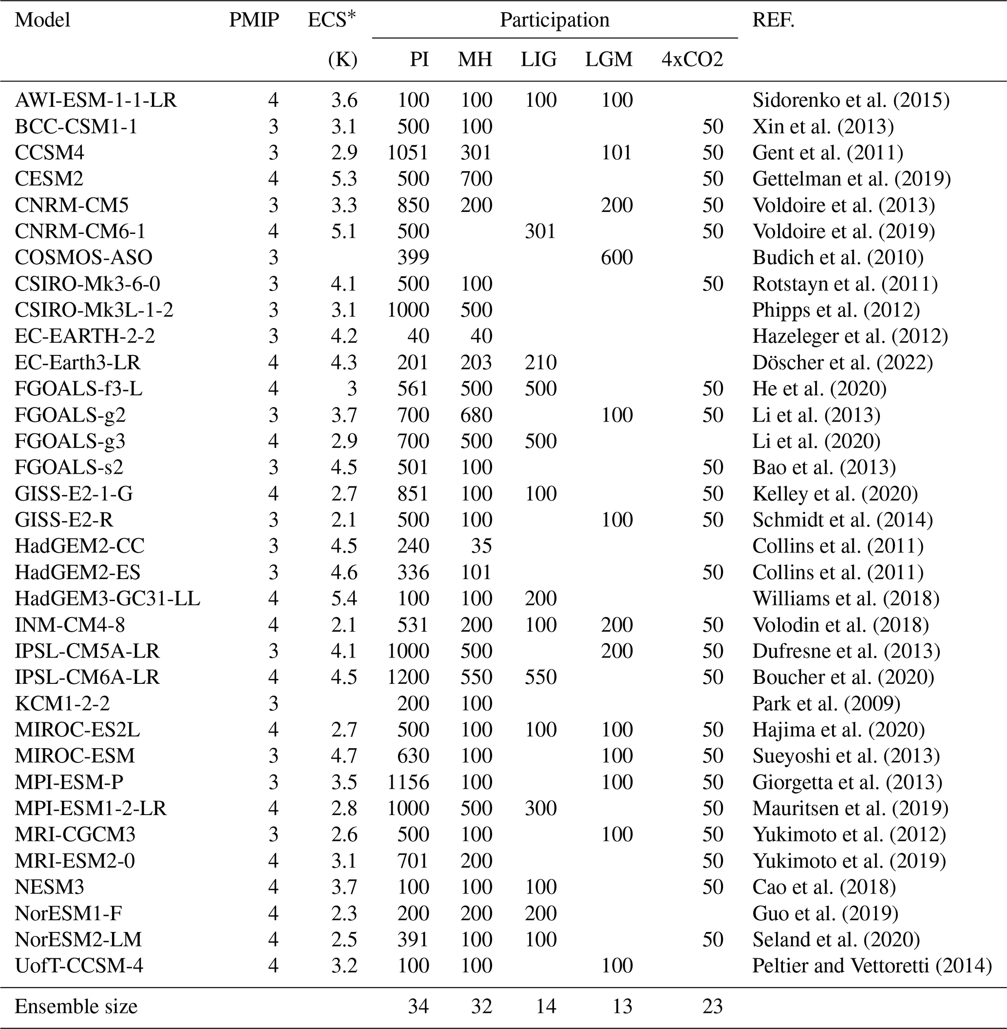
^∗ No values for the ECS of COSMOS-ASO and KCM1-2-2 were found.

2.1 Models

The CMIP has become a significant international multi-model research activity to investigate the Earth system response to forcing, evaluating the state-of-the-art coupled global climate models and assessing future climate changes and their uncertainties in scenarios (Eyring et al., 2016; Taylor et al., 2012). Simulations from the PMIP look at the past and serve as out-of-sample tests to study the roles of forcings and their feedbacks that establish the palaeoclimate and to evaluate the performance of models that are used to project future climate changes (Kageyama et al., 2018). Here, we choose the models that have completed the piControl simulations and at least one of the PMIP simulations (see Sect. 2.2) and have provided monthly surface temperature, precipitation and SLP for at least 30 years for all the simulations. Table 1 lists the 34 chosen models and their participation in the six experiments (see Sect. 2.2). Further details of the model design can be found in the listed references in Table 1 here, Table 9A.1 of Flato et al. (2013) for the CMIP5 models and Table AII.5 of IPCC (2021a) for the CMIP6 models.

2.2 Experimental design

This study uses simulations from five experiments with the protocols defined under the CMIP (Taylor et al., 2012; Eyring et al., 2016) or the PMIP (Kageyama et al., 2018): a PI control, one idealised CO₂-forced future warming experiment and three past climate experiments, which include a colder lgm and two altered orbital configurations midHolocene and lig127k. Model participation in each experiment is detailed in Table 1.

The DECK piControl was performed by all selected models, employing coupled atmosphere-ocean and boundary conditions approximately constant to 1850CE (Eyring et al., 2016). Depending on the individual model design, aerosol, vegetation, and ice sheet configurations are either interactive or prescribed as modern conditions. The CMIP6 piControl uses more realistic GHG concentrations (284.3 ppm, 808.2 ppb and 273 ppb for the atmospheric CO₂, NH₄ and N₂O concentrations, respectively) and a lower solar constant (1360.747 W m⁻²) compared to its earlier generation, the CMIP5, which set the atmospheric CO₂, NH₄ and N₂O concentrations at 280 ppm, 760 ppb and 270 ppb, respectively, and the solar constant at 1365 W m⁻². The piControl serves as a baseline for assessing changes in other experiments. Model groups run their piControl simulations for a few hundred to a few thousand model years to reach an equilibrium state.

The idealised CO₂-forced experiment, abrupt4xCO2, is also a requirement of the DECK CMIP experiments (Eyring et al., 2016). It is designed to reveal the basic feedback response of a model to high GHG forcing (Eyring et al., 2016) by having the atmospheric CO₂ concentration suddenly and immediately quadruple relative to the 1850 CE condition prescribed in the piControl at the beginning, and then maintaining constant (Eyring et al., 2016). The abrupt4xCO2 simulations enable the estimation of a model's equilibrium climate sensitivity (Zelinka et al., 2020). Its protocol remains unchanged as in the CMIP5, facilitating comparisons across CMIP generations.

The lgm experiment is designed to examine the effect of altered ice sheets, continental extent due to reduction in sea level, and lower GHG forcings (Kageyama et al., 2018). The concentrations of CO₂, NH₄ and N₂O are set to 190 ppm, 375 ppb and 200 ppb, respectively, in the PMIP4, and 185 ppm, 350 ppb and 200 ppb in the PMIP3. The major difference between the PMIP3 and PMIP4 lgm simulations is the choice of the prescribed ice sheets. While the PMIP3 simulations all used the same composite ice-sheet reconstructions (Abe-Ouchi et al., 2015), the PMIP4 simulations chose one of the three as summarised in Kageyama et al. (2021): the original PMIP3-CMIP5 ice sheet (Abe-Ouchi et al., 2015), GLAC-1D (Ivanovic et al., 2016) and ICE-6G_C (Peltier et al., 2015; Argus et al., 2014). Although these reconstructions have similar ice sheet extent, they differ in the heights of the Laurentide, Fennoscandian, and West Antarctica Ice Sheet.

The midHolocene and lig127k experiments are designed to examine the climate system responses to orbital forcings that differ from the PI (Kageyama et al., 2018). The experimental designs for the two experiments are outlined by Otto-Bliesner et al. (2017). In the PMIP4, the concentrations of CO₂, NH₄ and N₂O in the midHolocene experiment are set to 264.4 ppm, 597 ppb and 262 ppb, respectively, while those in the lig127k experiment are set to 275 ppm, 685 ppb and 255 ppb, respectively. The midHolocene, included since the beginning of the PMIP (Joussaume and Taylor, 1995; Braconnot et al., 2000), set to an orbital configuration at 6 ka following Berger (1978) and Berger and Loutre (1991). The orbit at 6 ka was characterised by larger obliquity, and its perihelion occurred near the boreal autumn equinox. The prescribed GHG concentrations in the PMIP4 midHolocene use more realistic concentrations derived from ice cores and observations (Otto-Bliesner et al., 2017) than the PMIP3, which contributes to a decrease of 0.3 W m⁻² in effective radiative forcing (Otto-Bliesner et al., 2017). The concentrations of CO₂, NH₄ and N₂O in the PMIP3 midHolocene experiment are set to 280 ppm, 650 ppb and 270 ppb, respectively. The lig127k uses the orbital configuration at 127 ka (Berger and Loutre, 1991), characterised by a larger eccentricity than the PI and its perihelion close to the boreal summer solstice. Both periods were characterised by receiving more insolation at the top of the atmosphere (TOA) in the Northern Hemisphere during June–July–August (JJA) and less incoming solar radiation in both hemispheres during DJF compared to 1850 CE, with the LIG having stronger orbital forcing than the MH.

2.3 Analysis and definitions

The analysis in this work follows the workflow described by Zhao et al. (2022). We create a curated replica of the relevant simulation outputs available on the System Grid Federation (ESGF; Balaji et al., 2018), which stores the CMIP6 outputs in a standardised format (Juckes et al., 2020). Digital Object Identifier (doi) for each simulation downloaded from the ESGF can be found in the Supplement. We also require some simulations from the model groups if they are not available on the ESGF. Then we apply calendar adjustment on the midHolocene, lig127k and lgm monthly output that re-aggregate the monthly output from a present-day calendar to those representing the past via the PaleoCalAdjust software by Bartlein and Shafer (2019).

The PMIP simulations do not have a fixed length. The length depends on when the simulations meet the criteria: (a) the absolute trend in global mean sea surface temperature is less than 0.05 K per century, and (b) the Atlantic meridional overturning circulatiom (AMOC) is stable (Kageyama et al., 2018). For the piControl experiment, CMIP6 requires a minimum of 500 years to ensure an equilibrium state (Eyring et al., 2016). For these equilibrium simulations, we take the average of the simulations (see Table 1 for the length of model years of each simulation). The CMIP protocol specifies a minimum length of 150 years for the abrupt4xCO2 simulations (Eyring et al., 2016). For consistency in our analysis, we take the last 50 years of the abrupt4xCO2 simulations for a direct comparison with other simulations employed in this study.

The Climate Variability Diagnostics Package (CVDP; Brierley and Wainer, 2018) had been modified for palaeoclimate purposes (Brierley and Wainer, 2018). We run the modified CVDP on each simulation to calculate multiple pertinent time series and spatial fields. The CVDP outputs have been regridded to 1° by 1° before analysing to eliminate the effects of different native resolutions across all the models. Multi-model mean anomalies take the average of regridded anomaly (experiment – piControl) across the ensemble members (Brierley and Wainer, 2018). Please see Zhao et al. (2022) for more details. We evaluate ensemble consistency via the threshold at which at least two-thirds of the models agree on the sign of the multi-model mean. Results of the PMIP4 and PMIP3 have not shown fundamental differences in statistics (Brierley et al., 2020; Kageyama et al., 2021), so we, therefore, combine the two indistinguishable phases in the purpose to enlarge the size of ensembles, which have been adopted in analysing ENSO (Brown et al., 2020) and Indian dipole (Brierley et al., 2023) across experiments.

Here, we adopt the definition of NAO as the leading EOF of DJF SLP anomalies over the Northern Hemisphere north of 20 to 80° N and 90° W to 40° E (hereafter referred to as the NAO pattern). The NAO index is the normalised PC time series of the EOF. Instead of using the NAO index, we use the amplitude of NAO to show its strength, which is measured as the standard deviation of the renormalised PC time series (i.e. the NAO index times the standard deviation of the spatial NAO pattern over the region). We also present spatial patterns associated with the NAO by linearly regressing the monthly temperature and precipitation onto the NAO index to evaluate the association between the NAO and surface climate variables (Brierley and Wainer, 2018). We also examine the similarity between the NAO and the Northern Annular Mode (NAM) in the PMIP experiments. All the experiments show that NAM and NAO are strongly correlated in the time series of the NAO indices, explained by variance and amplitude (not shown). Therefore, the following sections do not distinguish the NAO from the NAM.

3 Comparison with observations

Before looking at the response in experiments, we first evaluate the ability of the CMIP models used in this study to reproduce the North Atlantic climate states during the PI by comparing the piControl simulations with the C20 Reanalysis dataset (Compo et al., 2011), as shown in Fig. 1. Models generally capture the spatial pattern of observed mean DJF surface air temperature (SAT), but are biased in producing too cold Arctic, especially over Greenland and Nunavut (Fig. 1a, b). The cold bias has been detected by earlier PMIP analyses on a single experiment (Brierley et al., 2020; Otto-Bliesner et al., 2021), both showing a large spread across the models in Arctic regions between 60 and 90° N. The bias is partly associated with the model's representation of cloud radiative processes (Zhang et al., 2023) and atmospheric dynamics (Hall et al., 2021) and may also be affected by Arctic hydrography (Khosravi et al., 2022). Figure 1c and d show that models capture the DJF mean precipitation pattern over the North Atlantic Ocean, though they underestimate the amount of precipitation and shift the maximum location westward slightly as compared to the observation. The simulated SLP generally agrees with the observation (Fig. 1e, f), although it produces lower pressure along the coast of Greenland.

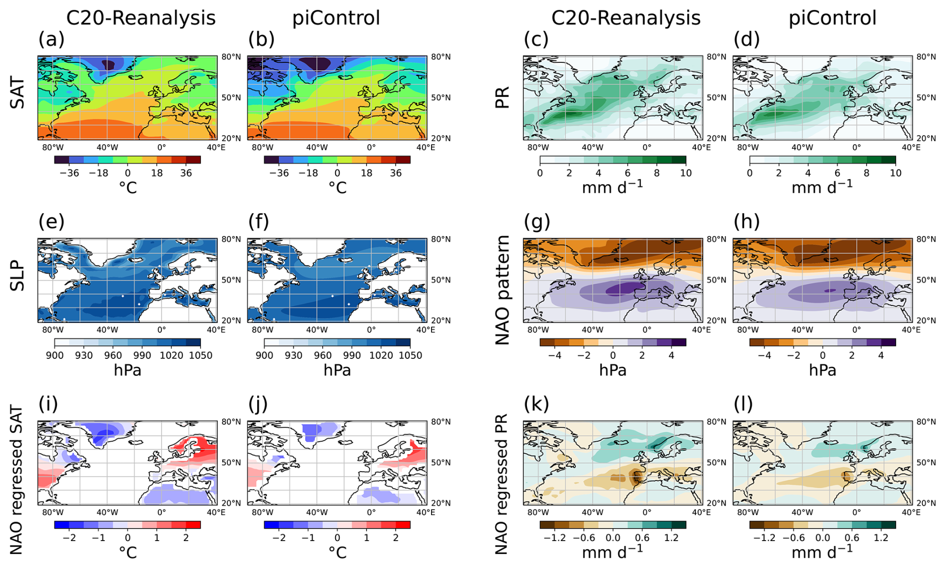
Figure 1 Comparison between observations taken from the 20th-Century Reanalysis (Compo et al., 2011) and the multi-model mean of the piControl simulations. Panels show DJF mean variables over the North Atlantic sector (see Sect. 2.3 for region definition). Panels present the (a, b) surface air temperatures in °C (SAT), (c, d) precipitation in mm d⁻¹ (PR), (e, f) sea level pressure in hPa (SLP), (g, h) NAO pattern in hPa, and teleconnections between NAO and (i, j) SAT in °C and (k, l) PR in mm d⁻¹ computed by regression against the NAO.

The NAO is the leading EOF of DJF SLP over the North Atlantic-Europe sector, showing a dipole structure with the negative anomaly over the northern centre and the positive anomaly over the southern centre (see Sect. 2.3). The piControl simulations show a distinguishable positive phase with a strong negative SLP centre over the northeast of Iceland and a positive centre over the northeast of the Azores (Fig. 1g, h). The simulated pattern shows such a dipole structure during the PI, which is consistent with observations, but the simulated negative anomalies extend further into the centre of Greenland, and the positive anomalies around 30–40° N North Atlantic Ocean are underestimated. Notably, 9 out of the 34 models display an eastward shifted positive centre over Europe along with varying degrees of pattern strength, and one model produces dipole positive centres over the Mediterranean and the central USA (not shown). In the piControl simulations, the NAO accounts for 41.5 % of the total variance (34.3 %–52.0 %; corresponding to the PI explained variance shown by the vertical range of black dots in Fig. 2a and the horizontal range of dots in Fig. 2b), slightly less than the 42.3 % observed in observational data (pink dashed lines in Fig. 2).

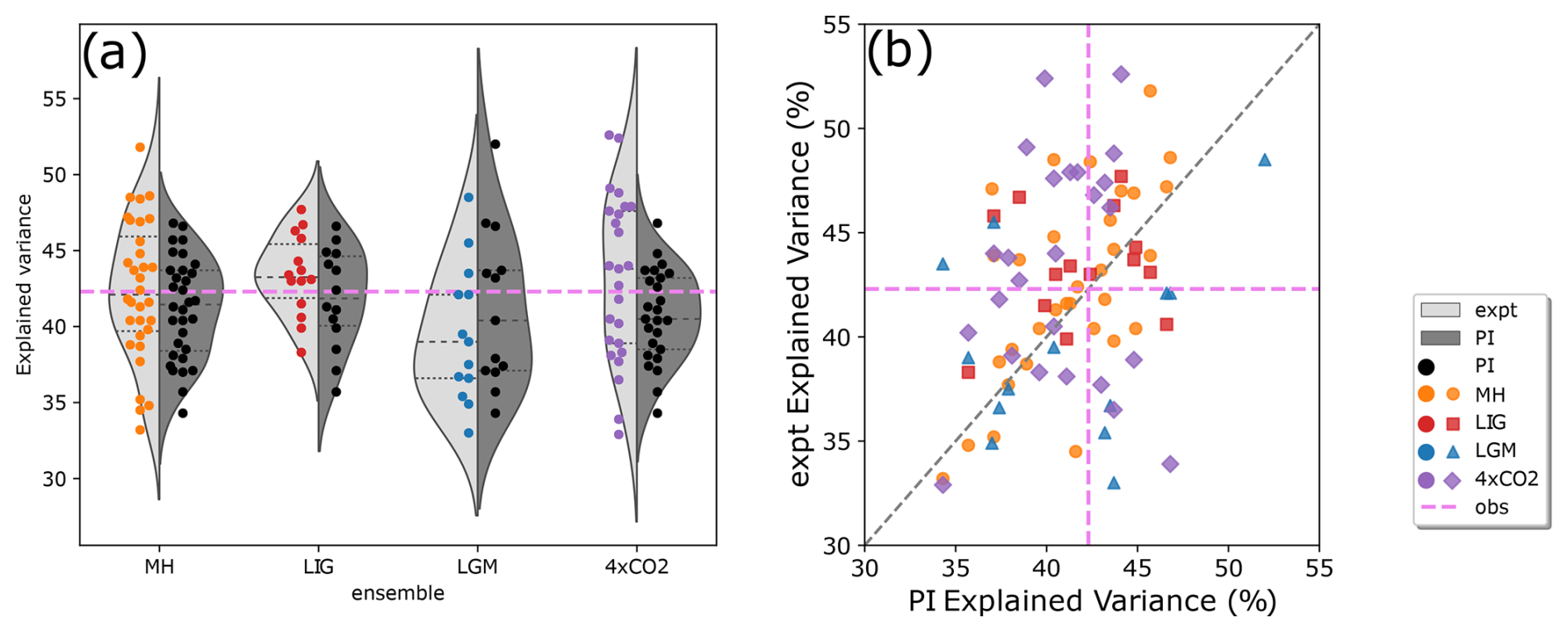
Figure 2 Total variance (%) explained by the NAO for (a) the experiments and (b) the models. Experimental names are abbreviated to MH for the midHolocene, LIG for the lig127k, LGM for the lgm, 4xCO2 for the abrupt4xCO2, and PI for the piControl, respectively. (a) For each column, the dots (corresponding to the left y-axis) show the explained variance by models. The distributions are computed via a kernel density estimation (Waskom, 2021): The curves and shading show the distributions of the explained variance by models for each experiment (left, shading in light grey) and the corresponding piControl (right, shading in dark grey); horizontal black dashed and dotted lines within each curve represent the median and 75 % and 25 % quartiles, respectively; pink dashed line across the panel represents the explained variance from the observation. The horizontal location of dots within each column has been offset for better visibility. (b) Each dot shows the comparison of the explained variance between the experimental simulation and the piControl by the model; pink dashed lines represent the explained variance from the observation.

The piControl SAT imprint of the NAO shows a pattern of warmer mid-latitudes and colder subpolar and subtropical regions than the observation (Fig. 1i, j), with the effect of a stronger jet stream located further north, stronger trade winds and northward shift of extratropical storms associated with a positive phase of NAO (IPCC, 2021b). The related northward shift of storm tracks with positive NAO phases results in a wetter northern Europe, a drier southern Europe and a northward shift of precipitation over the ocean. Both observations and models capture the pattern (Fig. 1k, l), but the simulated pattern is smoother than the observation with underestimated change magnitudes.

4 Change in mean state

Both the MH and the LIG were characterised by receiving less incoming solar radiation globally during DJF compared to 1850 CE, with a stronger reduction at 127 ka, suggesting an expectation of cooling in both experiments. The meridional SAT gradients of the midHolocene and lig127k experiments are weaker than the piControl, and the lig127k displays a stronger signal (Fig. 3a, d). The DJF mean temperature change averaged over the North Atlantic sector in the midHolocene experiment is 0.07 °C cooler than the piControl. The cooling is stronger in the lig127k experiment at −0.52 °C. Both experiments produce polar amplification, though the signal is inconsistent across the ensembles. The lig127k simulations show a large spread across the models in producing Arctic warming, and the midHolocene simulations show a larger ensemble spread over the whole region of the North Atlantic sector (Fig. 3a, d). The Euro-Atlantic precipitation fields show a drier Europe and an apparent drying off of the North American east coast in both experiments as compared to the piControl (Fig. 3b, e). There is a wetting over the rest of the Atlantic in the ensemble average, although the models do not all agree on the sign of the change. The signal of multi-model mean precipitation change is affected by NorESM2-LM, which produces a much larger precipitation increase north of 40° N than other models in both experiments. Figure 3c, f shows that SLP increases over lower latitudes and decreases over high latitudes.

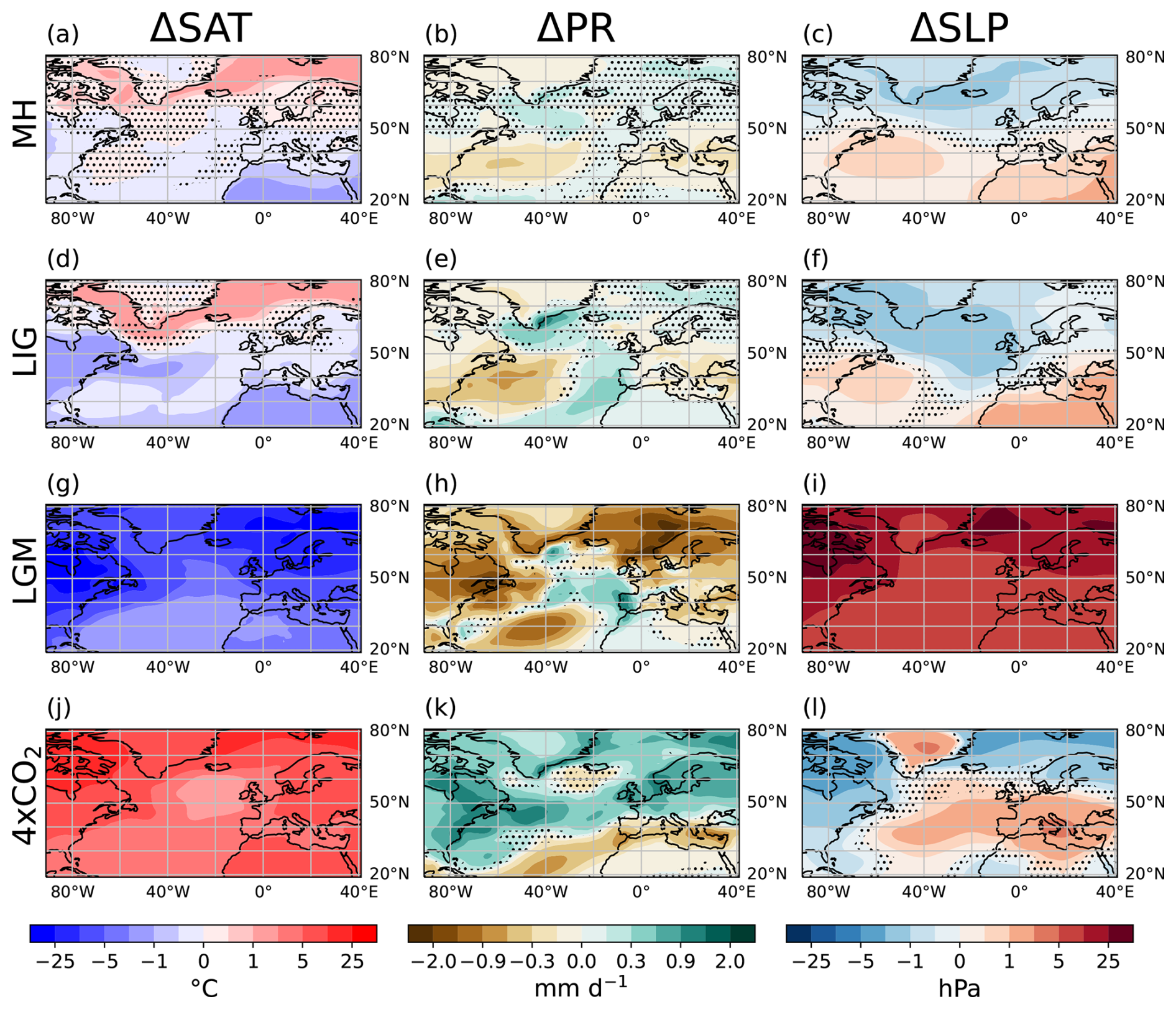
Figure 3 Multi-model mean change in mean states between experiments and the piControl. The columns from left to right show the DJF mean surface air temperature in °C (SAT; a, d, g, j), precipitation in mm d⁻¹ (PR; b, e, h, k), and sea level pressure in hPa (SLP; c, f, i, l). The rows from top to bottom represent the ensemble mean difference for the (a, b, c) midHolocene (MH), lig127k (LIG; d, e, f), lgm (LGM; g, h, i), and abrupt4xCO2 (4xCO2; j, k, l) experiments. Stippling indicates where the ensemble is inconsistent in the direction of change, i.e., at least two-thirds of the models disagree on the sign of the multi-model mean.

The Arctic warming during the boreal winter suggests other important processes, e.g., polar amplification with smaller and thinner sea ice in the Arctic (Serreze and Barry, 2011) and ocean memory (Marino et al., 2015; Govin et al., 2012). Meanwhile, neither of the two experiments (midHolocene and lig127k) incorporates some regional processes that can cause regional coolings. For example, the lig127k simulations did not include meltwater from ice sheets over Scandinavia and Canada related to the cooling in the Nordic Seas and south of Greenland shown by LIG reconstruction (Barlow et al., 2018; Otto-Bliesner et al., 2021). Earlier studies have compared the experiments with reconstructions and have confirmed that both experiments underestimate the Arctic warming (Brierley et al., 2020; Otto-Bliesner et al., 2021). The underestimated MH Arctic warming has existed since the PMIP3-CMIP5 (Harrison et al., 2015; Yoshimori and Suzuki, 2019). The regional temperature bias in the CMIP5 midHolocene, piControl and historical are similar (Ackerley et al., 2017; Harrison et al., 2015), which indicates the persistent errors in representing the climate system.

The LGM was characterised by a colder climate with a global mean cooling of 5–7 °C (Gulev et al., 2021) and large ice sheets covering the mid- to high-latitudes in the Northern Hemisphere (Clark and Mix, 2002; Clark et al., 2009). The averaged DJF cooling over the North Atlantic sector is −9.86 °C in the lgm simulations compared to the piControl. The lgm simulations show consistent cooling over the sector with a greater temperature decrease over land than over sea (Fig. 3g). The greatest cooling is found over the Norwegian and Barents Seas and parts of Scandinavia and North America, which reflects the change in surface height and albedo related to ice sheet change (Kageyama et al., 2021). The cooling is also partly affected by the advection of the cold temperature anomalies downwind of the ice sheets (Kageyama et al., 2021) and is partly related to a weakened AMOC (Jonkers et al., 2023). Though the cooling signal is consistent, the ensemble shows a large spread in simulating the magnitude of cooling affected by the choice of ice sheets of the PMIP3 simulations shown in Kageyama et al. (2021). Shi et al. (2023) decomposed the contributions of individual boundary conditions and forcings to the LGM cooling, finding that the cooling over the sea within the region is mainly due to the GHG forcings, and cooling over the continent is caused by changes in ice sheets. The lgm simulations show enhanced precipitation over the mid-latitudes of the North Atlantic Ocean as compared to the piControl, but the signal is not consistent across the ensemble (Fig. 3h). The SLP increases uniformly in the lgm simulations (Fig. 3i), consistent with the enhanced SAT cooling (Fig. 3g). The higher SLP over the polar regions, coupled with a cooler and drier climate, is related to the large Laurentide Ice Sheet (Otto-Bliesner et al., 2006).

The abrupt4xCO2 simulations contrast with the lgm, showing consistent warming across the whole North Atlantic region, with greater warming over land (Fig. 3j), amounting to 6.4 °C over the sector. The weakest warming appears over the ocean south of Iceland, where the surface current of the AMOC densifies and sinks to form deep water. Earlier studies suggest the AMOC weakening in the abrupt4xCO2 experiment in response to warming (Zhu et al., 2023; Madan et al., 2024). The switch of precipitation change signal represents a northward shift of the jet stream (Fig. 3k) relative to the piControl, whereas the inconsistency shows the uncertainty in producing the location of the jet stream, arising from both model bias and internal variability. Though the increase in the multi-model mean of abrupt4xCO2 precipitation change is consistent (Fig. 3k), the spatial pattern of the change by individual models is complex (not shown). The weakened precipitation south of Iceland is inconsistent across the abrupt4xCO2 ensemble (Fig. 3k), as about half of the models produce such a reduction. The pattern of abrupt4xCO2 SLP change (Fig. 3l) is not consistent with temperature change. The inactive prescribed Greenland Ice Sheet in simulations (Eyring et al., 2016) causes the SLP to increase over the region.

5 Change in NAO

The NAO patterns of the two orbital experiments (midHolocene and lig127k) are not distinguishable from the piControl (Fig. 4a, c). The similarity in the NAO pattern between the midHolocene and the piControl agrees with the findings of earlier modelling studies (Otto-Bliesner et al., 2006; Gladstone et al., 2005; Stephenson et al., 2006). It is also consistent with the PMIP2 simulations (Lü et al., 2010) that found the MH leading EOF of DJF SLP is similar to the PI. Models produce complex changes in the NAO pattern in both experiments and show a spread south of Greenland and Iceland near 50° N (Fig. 4b, d). Of the 32 models, 11 display a clear weakened, and 7 show an enhanced positive NAO phase in the midHolocene, respectively, as compared to the piControl; a similar result of spatial change occurs for the lig127k experiment, as 6 (5) out of the 14 models display weakness (enhancement) in the lig127k as compared to the piControl (not shown).

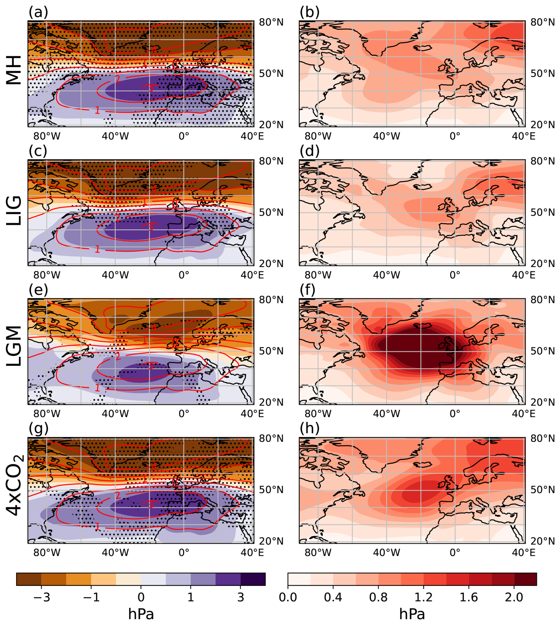
Figure 4 Multi-model mean DJF SLP spatial pattern for NAO (hPa) in each experiment (shadings, left column) and ensemble variation (right column), including the midHolocene (MH; a), lig127k (LIG; c), lgm (LGM; e) and abrupt4xCO2 (4xCO2; g). Red contours represent the pattern of the piControl, and stippling indicates where the ensemble is inconsistent in the direction of change. Ensemble variation is presented as the standard deviation across the ensemble (b, d, f, h).

The average percentage of explained variance during the midHolocene is 42.4 % (33.2 %–51.8 %), whose range is close to the piControl (Fig. 2a). The absence of clear changes in explained variance between midHolocene and piControl is consistent with Gladstone et al. (2005), which, in conjunction with inter-model inconsistencies, leads to uncertainties about the MH NAO behaviour. Changes in explained variance vary across the ensemble (Fig. 2b), ranging from −7.1 % to 10.1 %. In the lig127k simulations, models display an averaged explained variance at 43.4 % (38.3 % to 47.7 %), different from the 42.7 % (35.7 %–52.0 %) in the corresponding piControl simulations (Fig. 2a). Changes in explained variance by individual models vary across the ensemble and do not show a trend (Fig. 2b).

Figure 5 shows that the NAO amplitude in the midHolocene simulations is 2.31 hPa (0.77–3.15 hPa). The range and distribution of the midHolocene NAO amplitude is similar to those of the piControl (Fig. 5), though the differences between midHolocene and piControl by individual models range from −0.30 to 0.79 hPa. Though 19 out of 32 models present increased NAO amplitude, the ensemble mean change in the NAO amplitude is 0.06 hPa (Fig. 5). The slight increase is largely affected by 3 models, which contribute an intensification at 0.79, 0.50 and 0.43 hPa, respectively. The lig127k NAO amplitude is 2.18 hPa, similar to the piControl at 2.28 hPa with a more concentrated distribution (Fig. 5). The results of the two orbital-driven experiments suggest that the NAO response is unaffected by the seasonal variation induced by altered orbital configurations.

Figure 5 Same as Fig. 2a but for the NAO amplitude (hPa) for the experiments. The amplitude is measured as the standard deviation of the renormalised NAO PC time series (Sect. 2.3).

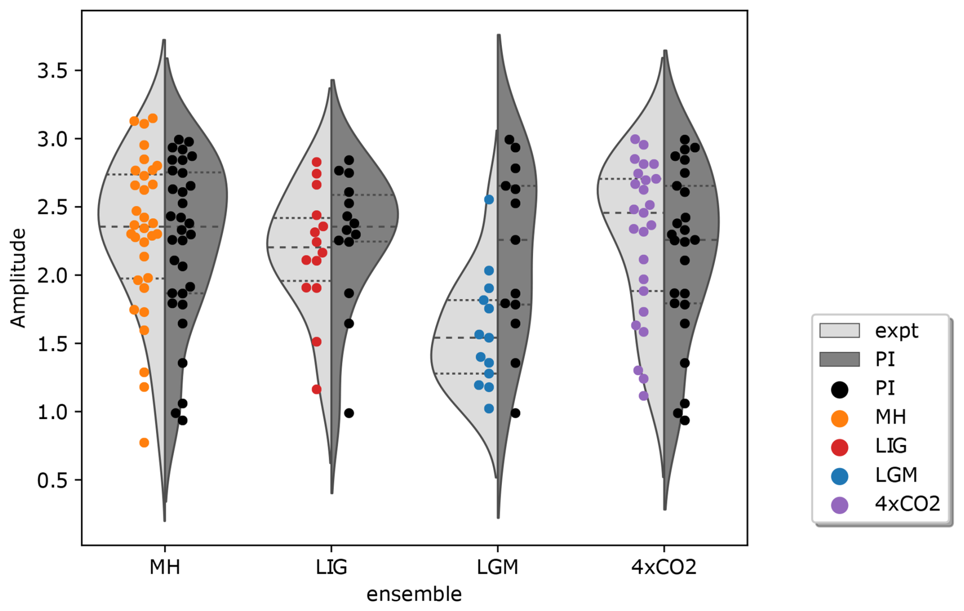
In the lgm experiment, the NAO is weaker as compared to the piControl (Fig. 4e). There is a southward shift of both the negative and positive centres of the NAO as compared to the piControl (Fig. 4e), though with a large model spread over the N. Atlantic Ocean between 40 and 65° N (Fig. 4f). The weakened NAO and centre shifts in the lgm are consistent with the results of Lü et al. (2010) and Otto-Bliesner et al. (2006). Models show large variations in producing the location of positive and negative centres of the NAO. 8 out of the 13 models display the switch of signal between 50 and 60° N, where a model displays its negative centre while another model shows its positive centre (not shown). The NAO explains 39.6 % (33 %–48.5 %) of SLP variability in the lgm that is −1.6 % less than the corresponding piControl simulations (Fig. 2a). The majority of the models show a reduction in explained variance (Fig. 2b), except three models show enhancements at 9.2 %, 8.7 % and 3.3 %. The lgm NAO amplitude is 1.58 (1.02–2.55) hPa, which is 0.59 hPa weaker than the piControl (Fig. 5), and one model contributes to the largest reduction in amplitude at −1.61 hPa. Only three models contribute to enhanced amplitude in the lgm simulations. Quartiles and median in Fig. 5 show a general reduction in lgm amplitude with respect to the piControl, which implies a weaker NAO in the lgm. The reduction is partly related to the presence of the Laurentide and Scandinavian Ice Sheets (Braconnot et al., 2007). Justino and Peltier (2005) suggested that these two ice sheets induce changes in the stationary waves, sea-ice extent and the oceanic meridional overturning circulation, which provides key context for the LGM NAO responses in this study.

The abrupt4xCO2 experiment shows the opposite change in the NAO pattern by showing enhancement and a slight northward shift in centres than the piControl (Fig. 4g, h). Models produce increased explained variance (Fig. 2) and stronger amplitude (Fig. 5) than the piControl. The abrupt4xCO2 simulations explain 43.2 % (32.9 %–52.6 %) of the SLP anomalies, which are 2.4 % (−12.9 % to 12.5 %) larger than the corresponding piControl simulations. Only 6 out of 25 models produce a reduction in explained variance, in which one model presents the largest reduction by −12.9 %, even larger than that in the lgm simulation at −4.7 % as compared to the piControl. The NAO amplitude in the abrupt4xCO2 experiment is 2.28 hPa on average (ranging from 1.12 to 3.00 hPa). Though the mean NAO amplitude of the abrupt4xCO2 is 0.11 hPa higher than the corresponding piControl, the median of abrupt4xCO2 NAO amplitude is slightly lower than that of the corresponding piControl (Fig. 5). Overall, the NAO is sensitive to GHG forcing and temperature change, as the warming strengthens the NAO, which implies that GHG changes in the future might play a role in modulating NAO behaviour.

As described in Sect. 1, the NAO variability is primarily driven by the internal variability of mid-latitude atmospheric dynamics (Lorenz and Hartmann, 2003). The findings of Rind et al. (2005a, b) show that both tropospheric and stratospheric climate changes influence the NAO response via altering propagating waves, angular momentum transport, and planetary wave energy. SST (Mosedale et al., 2006; Hurrell et al., 2004), GHG forcing (Stephenson et al., 2006; Barnes and Polvani, 2013), sea ice (Pedersen et al., 2016; Smith et al., 2017) and snow cover changes (Henderson et al., 2018; Spencer and Essery, 2016) could also be potential drivers. Rind et al. (2005b) stated that the Arctic Oscillation response during the Ice Age was dominated by changes in the eddy transport of sensible heat and local high-latitude forcing. Lü et al. (2010) examined the drivers of the NAO variability in the PMIP2 midHolocene and lgm experiments and found that the upward-propagating stationary Rossby waves might lead to NAO amplitude weakening. Based on four simulations, their midHolocene experiment presented a slight reduction in the Arctic Oscillation intensity. Our results show the opposite change as the NAO amplitude is slightly strengthened, but this finding is affected by a few models that produce a large enhancement. Our results of the lgm and abrupt4xCO2 experiments agree with the findings of Rind et al. (2005a, b), as the NAO increases under warmer states and decreases under colder states. They stated that the NAO index change is related to the eddy angular momentum transport change. The weakened lgm NAO amplitude is possibly due to cooler SST and reduced atmospheric moisture content as well as a shift of stationary waves and a weakened polar vortex linked to wave-mean flow interaction, and thus a reduction in polar westerlies (Lü et al., 2010). The internal variability is less important in contributing to model spread in this study, as the results are averaged over substantially longer periods (Sect. 2). The large model spread here is mainly attributed to the differences in model structure (McKenna and Maycock, 2021).

6 Associated Changes in the Climate Teleconnections

A positive NAO in the piControl is associated with warmer and wetter northern Europe and central North America and colder and drier Mediterranean and northern North America (Fig. 1j, l). Compared with the piControl, the midHolocene experiment shows a warmer continent associated with the NAO (Fig. 6a), with the warming extending farther into central Eurasia and central North America (not shown). Differently, the lig127k shows cooler conditions over northern North America and central Europe than the piControl (Fig. 6c). The DJF mean precipitation associated with the NAO increases over the North Atlantic Ocean north of 30° N and over northern Europe, while it decreases over central Europe and North America in the midHolocene (Fig. 7a). The lig127k experiment shows a similar pattern but with less precipitation over east of 20° W and north of 50° N relative to the piControl (Fig. 7c). However, mean changes in the DJF mean temperature and precipitation associated with the NAO are not robust in the midHolocene and lig127k as compared to the piControl, and the changes are not consistent across the ensembles (Figs. 6a–d and 7a–d). The MH models capture changes in the mean state (Fig. 3a) that project onto the positive phase of the NAO (Fig. 1h), as reconstructed by Funder et al. (2011). Proxy reconstructions also suggest that regional temperature patterns over Europe were primarily forced by a positive NAO-like phase during the MH as opposed to radiative responses forced by changes in the seasonal insolation cycle (Rimbu et al., 2003; Mauri et al., 2014). However, none of these papers include archives with sufficiently high temporal resolution to compare with the inter-annual variability being investigated here.

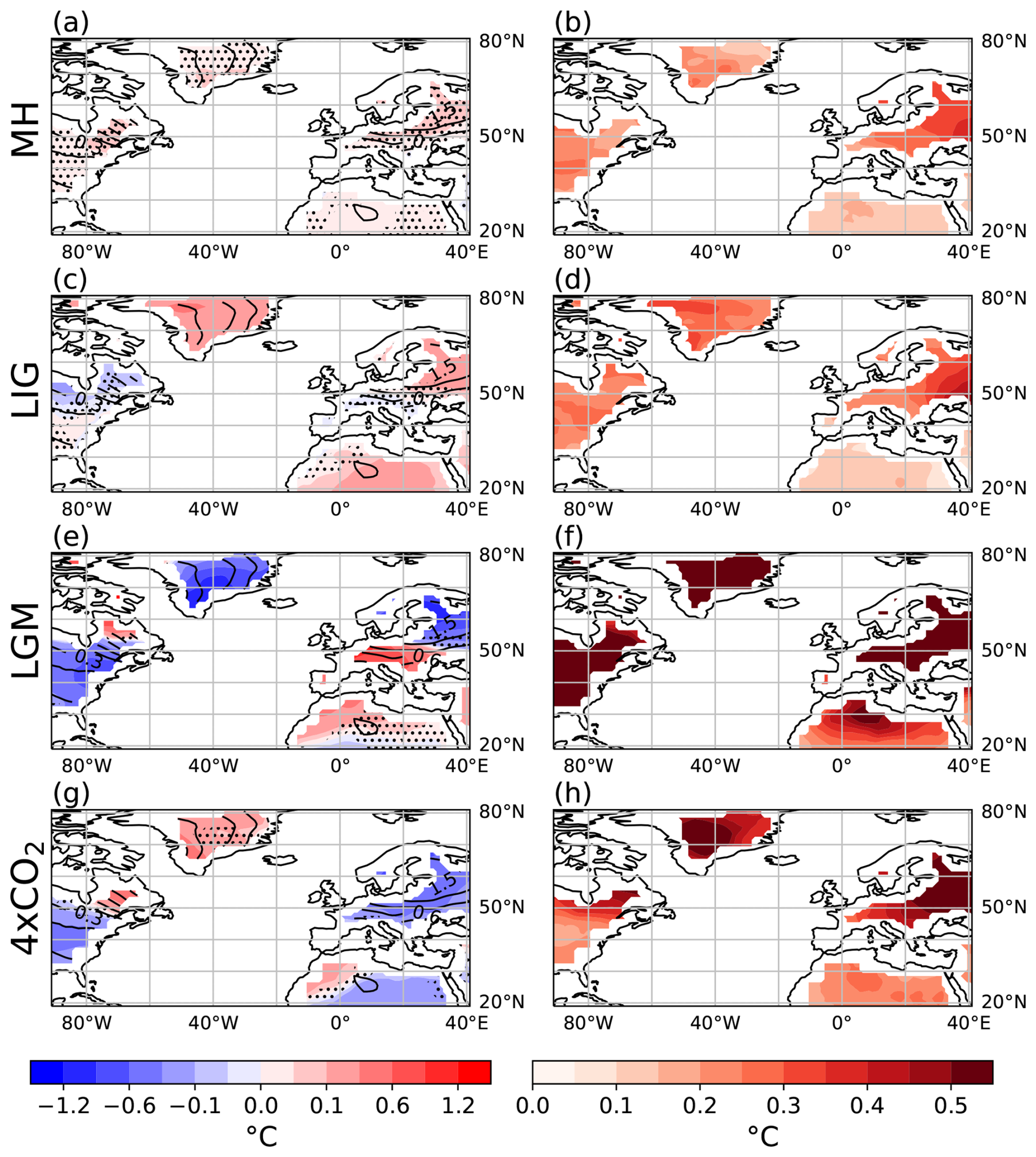
Figure 6 Multi-model mean change in DJF surface air temperature (°C) associated with the NAO as compared to the piControl (shadings, left column) and ensemble variation (right column). Experiments include midHolocene (MH; a), lig127k (LIG; c), lgm (LGM; e) and abrupt4xCO2 (4xCO2; g). Black contours show the pattern of the piControl. Stippling indicates where the ensemble is inconsistent in the direction of change. Ensemble variation is presented as the standard deviation across the ensemble (b, d, f, h).

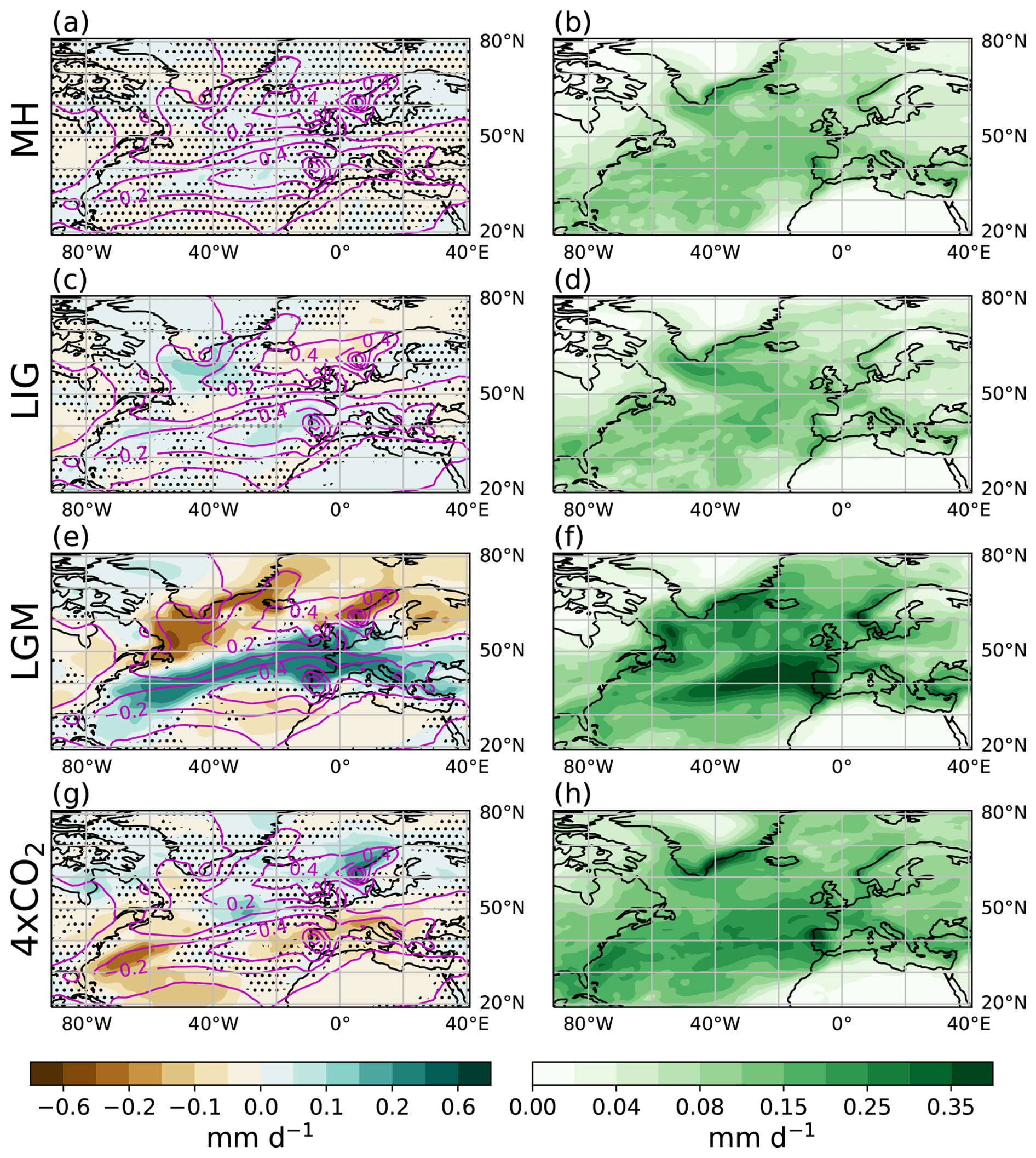
Figure 7 Same as Fig. 6 but for muti-model mean change in DJF precipitation (mm d⁻¹) associated with the NAO. Magenta contours show the pattern of the piControl. Stippling indicates where the ensemble is inconsistent in the direction of change.

The temperature and precipitation patterns associated with the NAO shift southward in the lgm experiment (Figs. 6e and 7e), which suggests a reduction of features of the positive boreal winter NAO. Associated with the NAO, the lgm experiment presents colder and drier central North America and northern Europe and warmer and wetter Mediterranean and northern North America than the piControl, with the patterns extending to central continents (not shown). As the strengthened precipitation teleconnection pattern over the western Iberian Peninsula is also present in the mean-state change (Fig. 3h), it suggests that the strengthened Mediterranean precipitation pattern is not necessarily directly forced by the NAO. In the abrupt4xCO2 experiment, opposite to the lgm, features of the positive boreal winter NAO are enhanced compared to the piControl (Figs. 6g and 7g). The associated changes in temperature and precipitation do not match the pattern and magnitude of robust change in mean state temperature and precipitation (Fig. 3), which implies that changes have less influence on change in mean state climatology in the NAO and have other attributions. For example, the large ice sheets during the LGM limited turbulent air-sea heat fluxes in the high-latitude North Atlantic that influenced the NAO and cooled the temperature (Sect. 4). The warming in the abrupt4xCO2 can be explained by the thermodynamic processes affecting heat and moisture transport without changing the large-scale atmospheric circulation patterns (Stephenson et al., 2006). The enhanced warming of the surface boundary layer enhances vertical latent heating, which in turn influences the atmospheric moisture content and baroclinic stability (Lorenz and DeWeaver, 2007).

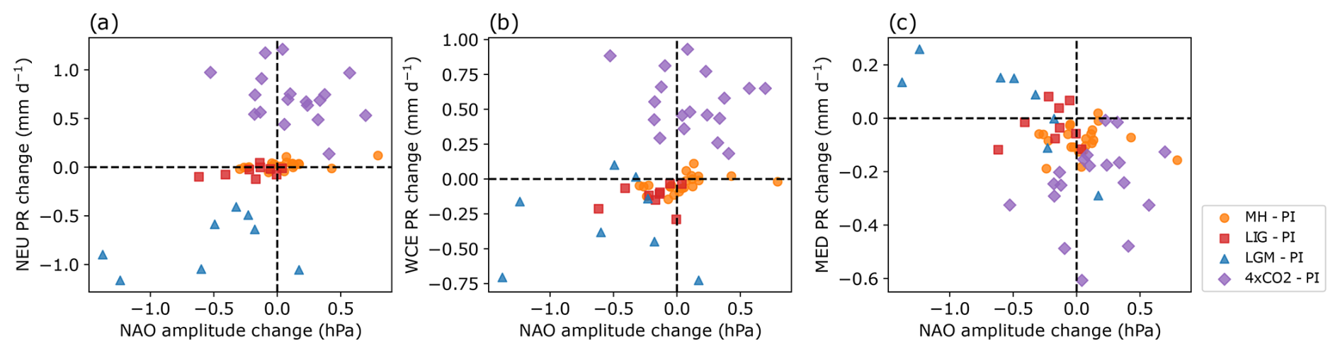
Figure 8 Relationships across all experiments and all models between the changes in NAO amplitude and the changes in European mean state of DJF mean precipitation (mm d⁻¹; labelled as PR in panels a to c). Regions follow the definition of IPCC AR6: northern Europe (NEU), west and central Europe (WCE), and Mediterranean (MED). All changes are relative to the piControl.

NAO greatly impacts the European climate (Sect. 1). Figure 8 shows the relationships between the changes in NAO amplitude and changes in DJF mean precipitation over northern Europe, central Europe, and the Mediterranean relative to the piControl. The change in NAO amplitude is found to have positive correlations with the change in DJF mean precipitation over northern and central Europe (Fig. 8a, b) and a negative correlation over the Mediterranean (Fig. 8c). The lgm experiment displays a weakened NAO amplitude along with colder mean temperatures, while the other three experiments do not show a clear relationship between the change in NAO amplitude and the temperature change (not shown). Terrestrial proxy data suggest a warmer winter in Europe during the MH (Bartlein et al., 2011) and the LIG (Brewer et al., 2008). However, models do not capture this warming in Europe in both experiments and even present a uniform cooling in the lig127k. Mauri et al. (2014) suggested that models do not capture a positive NAO-like pattern due to failing to capture the full extent of high-latitude warming over Northern Europe and underestimate the cold Mediterranean temperatures. This might indicate that the changes in climatological sea level pressure (Fig. 3 right column) are underestimated in the ensemble. Notably, our findings should be interpreted alongside the perspective from Hurrell et al. (2003): although NAO is the dominant mode of atmospheric circulation variability over the North Atlantic, it explains only a fraction of the total variance, and most winters cannot be characterized by the canonical NAO pattern. This implies that while our results highlight NAO's sensitivity to GHG forcing and temperature changes, the actual contribution of NAO variability to European climate may be constrained by its limited explanatory power of total circulation variance.

Earlier studies have noticed a teleconnection existing between ENSO and NAO (Geng et al., 2024; Toniazzo and Scaife, 2006; Hardiman et al., 2019; Zhang et al., 2015; Joshi et al., 2021), though it remains controversial with large uncertainty (López-Parages et al., 2015; Zhang et al., 2019). The ENSO signals reach the North Atlantic region via the stratosphere (Ineson and Scaife, 2009) and tropospheric pathways (Jiménez-Esteve and Domeisen, 2018). Here we investigate whether a weakened/strengthened ENSO could remotely influence the NAO amplitude. The NAO-ENSO relationship responds nonlinearly to changes in ENSO strength (Hardiman et al., 2019). Enhanced ENSO events affect NAO variability by exciting Rossby waves reaching the North Atlantic through strengthened convection anomalies in the Gulf of Mexico and the Caribbean Sea (Ayarzagüena et al., 2018) and in the tropical Indian and Pacific Ocean (Abid et al., 2021; Joshi et al., 2021). Here, we examine the relationship between change in the strength of ENSO, measured as the standard deviation of nino3.4 index, and change in NAO amplitude (Fig. 9). Consistent with Brown et al. (2020), ENSO strengths in the two orbital-forced experiments are weakened (more obviously in the lig127k experiment), while they are ambiguous in the lgm and abrupt4xCO2 (Fig. 9). In contrast, the NAO amplitude weakens in the lgm and its changes are ambiguous in the abrupt4xCO2, midHolocene and lig127k experiments (Fig. 9). There is no clear relationship between the amplitude changes of ENSO and NAO (Fig. 9). It implies that changes in ENSO strength do not remotely influence the NAO amplitude and, therefore, suggest a more nuanced teleconnection than posited by earlier studies.

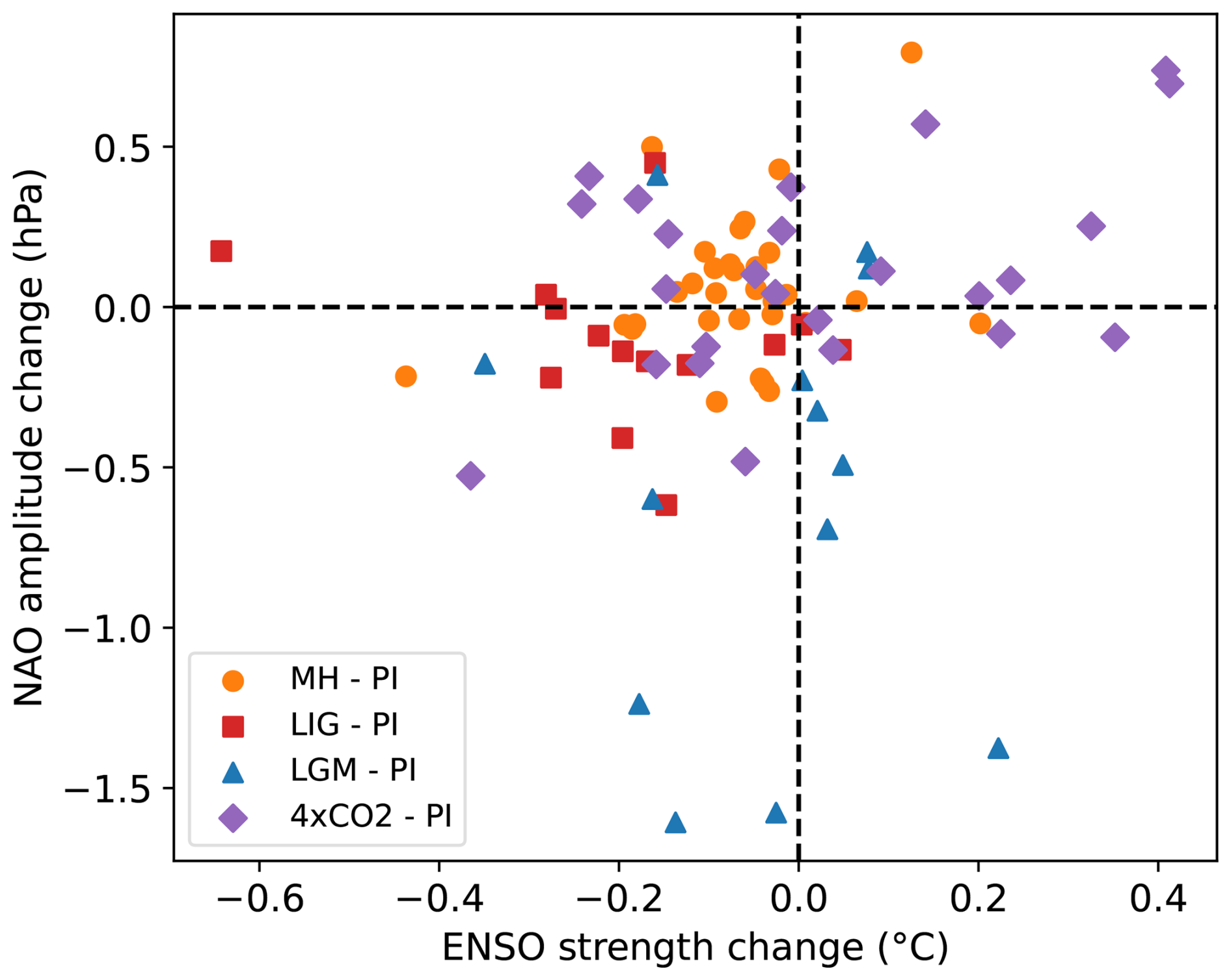
Figure 9 Relationship between the change in ENSO strength and NAO amplitude across all models and all experiments relative to the piControl. The ENSO strength is measured as the standard deviation of the nino3.4 index of each simulation.

7 Conclusions

We assessed changes in NAO amplitude and teleconnections in a combination of CMIP5 and CMIP6 models. The simulations for past climates include two altered orbital configurations at the MH (midHolocene) and LIG (lig127k) and a colder-than-present LGM (lgm), and an idealised GHG-forced warming experiment of abrupt quadrupling of CO₂ (abrupt4xCO2). For model evaluation, we compared the piControl simulation with the C20 Reanalysis dataset (Compo et al., 2011), as shown in Sect. 3. The piControl ensemble reproduces the observed mean state, but with biases. The patterns of the positive phase of the NAO and associated teleconnections are consistent between observation and the piControl but with variations across the simulations. We explored changes in NAO spatial patterns and explained variance and amplitude. NAO weakens in response to cooling and strengthens as a result of warming. Some of our results are inconsistent with earlier studies, but the inconsistencies are likely affected by the outputs of a few models. The underlying mechanisms are unclear, but previous studies have highlighted the influence of tropospheric and stratospheric climate changes on NAO behaviour (Rind et al., 2005a, b; Lü et al., 2010). We also discussed changes in NAO teleconnections. The simulated spatial teleconnection patterns associated with the NAO are generally consistent with the theory (see Sect. 1) and are sensitive to the change in NAO amplitude. The midHolocene and lig127k experiments do not show a clear change in temperature and precipitation associated with the NAO. The weakened NAO in the lgm is associated with a cooler and drier northern Europe, while the enhanced NAO in the abrupt4xCO2 is associated with a warmer and wetter northern Europe as compared to the piControl. We did not find the ENSO-NAO teleconnection suggested by other studies. Further work is required to fully understand the underlying mechanisms driving the NAO change and the associated teleconnections.