Simulating global ice volume across the Mid-Pleistocene Transition with a ramp-like increase in the deglaciation threshold

During the Quaternary period, spanning the last 2.6 million years, the characteristic frequency and amplitude of glacial-interglacial cycles evolved from low-amplitude 41 000-year cycles to high-amplitude 100 000-year cycles. This transition occurred around 1.2 to 0.8 million years ago and is referred to as the Mid-Pleistocene Transition (MPT). The absence of any significant change in the external orbital forcing during this period suggests the existence of some fundamental change within the Earth-climate system, leading to non-linearities or feedback mechanisms. The temporal structure of such a change is still under debate. Here, we present a new conceptual model of the Quaternary global climate, the so-called RAMP model, which can reconstruct the past global ice volume. The RAMP model incorporates a ramp-like change in its deglaciation threshold to reconstruct the MPT. Parameter optimization finds that the onset of the change occurs in the early Quaternary (2.6–2.3 Ma) and lasts into the 100 kyr world (550–250 ka). These findings support the idea of a long-term shift as a cause of the MPT and imply that the climate shift began early in the Quaternary. The model uses a linear combination of the precession parameter and obliquity as external orbital forcing, which can be optimized to best reconstruct the target curve. The identified orbital forcing differs from the widely used insolation at summer solstice at 65° N, as the latter exhibits a larger precession signal. The RAMP model yields consistent and good results for two different global mean sea level curves. Moreover, we conduct a series of sensitivity tests, in which the RAMP model demonstrates strong robustness. In particular, the identified long-lasting period for the ramp is a very robust feature of the model, underscoring its key role in reconstructing the MPT.

1 Introduction

The Quaternary is the most recent geological epoch, covering the last 2.6 Ma. It is characterized by the alternation of cold glacial climate states and warmer interglacial periods. In the first half of the 20th century, Milutin Milankovitch made significant contributions to the astronomical theory of climate, which links changes in Earth's orbital parameters to changes in the radiative forcing, which ultimately leads to glacial-interglacial variability (Milankovitch, 1941). Earth's obliquity varies on a cycle of approximately 41 kyr, while precession operates over a 19 kyr and a 23 kyr period, and eccentricity fluctuates on a 100 kyr and a 400 kyr timescale (Hays et al., 1976). In his theory, the orbital variations of Earth's eccentricity, obliquity and precession lead to variations in the insolation during boreal summer, which is the dominating driver of glacial cycles (Ganopolski, 2024).

Two central problems arise from this theory. The first is known as the 100 kyr problem: the late Quaternary glacial cycles (approximately the last 800 ka) follow 100 kyr patterns, despite the eccentricity having only a negligible influence on the global insolation compared to the obliquity and precession (Raymo and Huybers, 2008; Imbrie et al., 2011; Barker et al., 2022). The second issue is related to the shift of low-amplitude ∼ 41 kyr cycles towards high-amplitude ∼ 100 kyr cycles during the mid-Pleistocene (∼ 1.2–0.8 Ma) in the absence of any significant change in orbital forcing. This transition is known as the Mid-Pleistocene Transition (MPT) (Imbrie et al., 2011; Barker and Knorr, 2023; Elderfield et al., 2012). The occurrence of the MPT poses one of the most challenging open questions to the paleoclimatological community and has been the subject of intense studies (Willeit et al., 2019; Legrain et al., 2023; Berends et al., 2021b; Ganopolski, 2024). Various internal feedback mechanisms of the climate system and non-linearities have been put forward to explain this major climatic shift (Legrain et al., 2023; Berends et al., 2021b).

Recent studies suggest that the duration and timing of deglaciation and glaciation events over the last 900 ka were largely deterministic and driven by the relative phasing of precession, obliquity, and eccentricity (Barker et al., 2022, 2025). Barker et al. (2025) identified candidate precession peaks, which are precession peaks that begin while obliquity is increasing, as essential for glacial terminations. They found that all glacial terminations during the last 900 ka correspond to the first candidate precession peak after a minimum in eccentricity. This is how the 100 kyr periodicity comes into play for the post-MPT world. On the other hand, it seems like obliquity alone controls the following glacial inception, which is triggered by the start of its next decreasing phase. During and prior to the MPT, the authors found that almost all candidate precession peaks are linked to glacial terminations. Since they depend on rising obliquity values, they are mainly paced by obliquity, resulting in the observed 41 kyr world with no more influence of eccentricity on these cycles. This leaves open the question of why there was a change in the climate response to candidate precession peaks.

While various hypotheses have been proposed to explain the MPT, the following two are particularly popular. The regolith hypothesis suggests that gradual removal of thick regolith layers (10–50 m) on the North American and Eurasian surface during continuous glaciations exposed the high-friction crystalline bedrock underneath, reducing basal ice flow and increasing ice sheet stability, leading to the observed 100 kyr periodicity (Clark and Pollard, 1998; Clark et al., 2006; Willeit et al., 2019). Alternatively, a gradual cooling trend, associated with a decrease in atmospheric CO₂ concentrations throughout the Quaternary, may have triggered the MPT (Scherrenberg et al., 2025). Based on such a long-term cooling trend, various feedback mechanisms in the ice sheet or changes in the ocean circulations have been proposed as a secondary trigger for the MPT (Berends et al., 2021b).

Another open question concerns the temporal structure of the change that might have triggered the MPT. While a gradual scenario involves a linear change over the entire Quaternary (like the CO₂ hypothesis), a more abrupt scenario involves the crossing of some irreversible climatic thresholds over a short period of time (Legrain et al., 2023). One proposed abrupt mechanism involves non-linear feedback effects from the merging of the North American Laurentide and Cordilleran ice sheets (Berends et al., 2021b; Bintanja and van de Wal, 2008; Gregoire et al., 2012).

Moreover, the effects of the MPT on the evolution of global ice volume across the Quaternary remain incompletely understood, as there are currently two contrasting views. The reconstruction of global ice volume is based on benthic foraminifera δ¹⁸O_b, measured in marine records. It consists of two components, a temperature δ¹⁸O_T and a seawater δ¹⁸O_sw component, with the latter serving as a proxy for global ice volume. One common approach to disentangle these two components from the δ¹⁸O_b signal is to apply some kind of regression method. This approach largely reproduces the variability present in the δ¹⁸O_b signal, resulting in small ice sheets in the early Pleistocene, which increase in volume after the MPT. In contrast, a recent study by Clark et al. (2025b) deconvolved δ¹⁸O_b into its seawater δ¹⁸O_sw component, based on ocean temperature data, and subsequently Clark et al. (2025a) applied a mass-balance approach to this δ¹⁸O_sw record, considering time-varying temperature and ice volume effects on the δ¹⁸O of ice sheets, to reconstruct the Global Mean Sea Level (GMSL) over the past 4.5 Ma. This reconstruction no longer shows an increase in global ice volume over the Pleistocene, but just a transition in glacial frequency. Furthermore, this curve exhibits large ice sheets around 2.5 Ma, which is in better agreement with terrestrial (Balco and Rovey, 2010) and marine (Shakun et al., 2016; Rea et al., 2018) evidence. So at present, there are two fundamentally distinct perspectives on how global ice volume varied throughout the Pleistocene and on how the MPT affected the global ice volume variability.

Climate models present a versatile tool for investigating these different hypotheses and open questions. They range from computationally expensive Earth System Models to simple, zero-dimensional (spatial dimensions) conceptual models that focus on key variables while allowing long simulations. Simple models rely on a reduced number of highly aggregated macroscopic variables that try to reconstruct the full dynamics as closely as possible (Saltzman, 2001). Various conceptual models have been developed over the last few decades, varying in their underlying assumptions and hypotheses. Many of them yield good results and can reconstruct the 100 kyr world with its characteristic saw-tooth pattern (Gildor and Tziperman, 2001; Imbrie et al., 2011; Parrenin and Paillard, 2012; Pérez-Montero et al., 2024) or even the MPT with its shift in amplitude and frequency and its specific timing (Paillard, 1998; Paillard and Parrenin, 2004; Legrain et al., 2023; Ganopolski, 2024).

A common approach is to attribute glacial-interglacial variability to relaxation oscillations between multiple equilibria (Paillard, 1998; Parrenin and Paillard, 2012; Legrain et al., 2023; Leloup and Paillard, 2022). In his initial work, Paillard (1998) proposed a three-state model (hereafter referred to as P98) consisting of an interglacial, mild glacial, and a full glacial state. Transitions between model states depend on the ice volume and the insolation. To account for a change in forcing due to decreasing atmospheric CO₂ concentrations, he added a small linear trend in the radiative forcing and linearly increased one of the state thresholds. This model is able to simulate the global ice volume over the past 2 Ma, with good results in the timing of terminations and the change in periodicity due to the MPT. In later work, Parrenin and Paillard (2012) presented an improved version of this model (hereafter referred to as PP12), which only consists of a glaciation and a deglaciation regime. While the deglaciation trigger depends on a combination of ice volume and insolation, the glacial inception is solely controlled by insolation. Moreover, they adapted the solar forcing, such that the model takes a linear combination of three functions of orbital parameters instead of a fixed insolation curve. A similar approach was used in the model of Imbrie et al. (2011). Indeed, the model results seem to depend on the chosen insolation forcing, since they differ in their contributions from obliquity and precession (Leloup and Paillard, 2022). The three model versions by Legrain et al. (2023) (hereafter referred to as L23 models) continued the work by implementing different internal forcing scenarios to test which of them is most likely to reproduce the MPT. In addition to the external solar forcing, they added internal variations to the model in the form of a varying deglaciation threshold. They found that a gradual increase of this deglaciation threshold is more likely to reproduce the MPT than an abrupt change. Based on this finding, they suggested that a gradual decline in atmospheric CO₂ concentrations over the Pleistocene may have increased the deglaciation threshold, potentially causing the MPT.

Imbrie et al. (2011) proposed a phase-space model that again combines ice volume and orbital forcing as a deglaciation trigger. They were able to reproduce the shift in frequency of glacial-interglacial cycles purely by orbital forcing, without changing any model parameters during the MPT. Hence, they linked the occurrence of 100 kyr glacial cycles to the eccentricity-driven amplitude modulation of precession. However, their model-data comparison was limited to a detrended benthic δ¹⁸O curve rather than an ice volume reconstruction, thereby precluding the assessment of whether their model accurately reconstructs the change in amplitude over the MPT.

In a more recent work, Ganopolski (2024) attempted to set up a generalized Milankovitch Theory by incorporating model results from CLIMBER-2 (a more sophisticated Earth-System Model) into a conceptual model. The model can reproduce the glacial cycles of the Quaternary based on the nonlinear response of the climate system to the orbital forcing in the form of the eccentricity-driven amplitude modulation of precession and the existence of supercritical ice sheets. A gradual increase in the critical ice volume is added to model the MPT. The author associates this with the gradual removal of terrestrial sediments in the Northern Hemisphere (NH), which is needed to prolong the late-Pleistocene glacials.

In this study, we improve the 2-state L23 conceptual models. To account for potential feedback mechanisms in the climate system or internal changes in the system, we implement a new ramp-like scenario, called the RAMP model. Here, the focus lies on the general temporal structure of such a change, allowing for its physical interpretation. The RAMP model covers all three temporal scenarios discussed in the L23 models and is characterized by its easy adjustability. In comparison with the L23 models, it can be run on different time scales, simulated into the future, reconstruct different global ice volume curves, and can be easily re-tuned for new parameterizations (e.g. allowing to test the effects of changes in the state thresholds, forcing, etc.). Since the precursor L23 models were designed to simulate an increase in global ice volume amplitude over the MPT, we use the GMSL reconstructions of Berends et al. (2021a) and Rohling et al. (2022) as target curves, instead of the recent reconstruction by Clark et al. (2025a). An adjusted model version, the RAMP-2 model, which can simultaneously reconstruct the Berends and Clark curves, is presented in the Supplement (Sect. S7) and discussed in Sect. 4.4.

2 Methods

2.1 RAMP model

The new RAMP model presents an improved version of the L23 models. In the following, the model formulation is described. A detailed description of the changes compared to the L23 models can be found in the Supplement (Sect. S1).

The RAMP model uses orbital forcing as an input to reconstruct the global ice volume over the Quaternary. Leloup and Paillard (2022) showed that the model outcome depends on the chosen insolation forcing, which differ in their precession and obliquity signals (e.g. summer solstice or caloric summer half-year insolation at 65° N). Hence, the subjective modelling choice of selecting a specific insolation metric, determines the strength of the precession and obliquity signals in the model. Some earlier models (Imbrie et al., 2011; Parrenin and Paillard, 2012; Legrain et al., 2023) use instead a linear combination of the precession and co-precession parameters and obliquity, which can represent insolation at most latitudes and seasons (Imbrie et al., 2011). In the RAMP model, we only use a linear combination of the precession parameter and obliquity. We show that such a linear combination of only two functions of orbital parameters can indeed accurately reconstruct various insolation curves (Sect. S4). The following functions of orbital parameters (normalized and dimensionless) from La2004 orbital solution (Laskar et al., 2004) are used:

$$\begin{array}{}\text{(1)}& {\displaystyle }\text{Esi}:\text{Precession parameter}\sim e\sin \left(\mathit{\omega }\right),\text{(2)}& {\displaystyle }\text{Ob}:\text{Obliquity}\sim \mathit{ϵ},\end{array}$$

with ω the precession angle taken from the vernal equinox and e the eccentricity.

Hence, the global ice volume change per unit time in response to the orbital forcing I(t) (m kyr⁻¹) is defined in the model as:

$$\begin{array}{}\text{(3)}& I\left(t\right)={\mathit{\alpha }}_{\mathrm{Esi}}\text{Esi}\left(t\right)+{\mathit{\alpha }}_{\mathrm{O}}\text{Ob}\left(t\right),\end{array}$$

with the constant weights α_Esi and α_O (m kyr⁻¹). For brevity, we will refer to I(t) simply as the orbital forcing from here on.

The model has two different regimes, the glaciation (g) and the deglaciation regime (d). Depending on the current model regime, the global ice volume v(t), given in meter sea level equivalent (m sl), is driven by two first-order differential equations:

$$\begin{array}{}\text{(4)}& {\displaystyle }g:{\displaystyle \frac{\mathrm{d}v\left(t\right)}{\mathrm{d}t}}=-I\left(t\right)+{\mathit{\alpha }}_{\mathrm{g}},\text{(5)}& {\displaystyle }d:{\displaystyle \frac{\mathrm{d}v\left(t\right)}{\mathrm{d}t}}=-I\left(t\right)-{\displaystyle \frac{v\left(t\right)}{{\mathit{\tau }}_{\mathrm{d}}}},\end{array}$$

where α_g (m kyr⁻¹) is a constant model parameter controlling the glacial rate of advance and τ_d (kyr) is the constant relaxation time, which controls the deglacial rate of retreat.

A state change from a glaciation to a deglaciation (g) → (d) occurs when a combination of the current ice volume v(t) and the orbital forcing exceeds a critical threshold:

$$\begin{array}{}\text{(6)}& \left(\text{i}\right)v\left(t\right)\cdot \stackrel{\mathrm{̃}}{I}\left(t\right)+v\left(t\right)>v_{\mathrm{0}}\left(t\right)\text{and}\left(\text{ii}\right)v\left(t\right)\cdot \stackrel{\mathrm{̃}}{I}\left(t\right)>v_{\mathrm{1}}.\end{array}$$

Vice versa, a transition from a deglaciation to a glaciation state (d) → (g) occurs when:

$$\begin{array}{}\text{(7)}& \left(\text{i}\right)v\left(t\right)\cdot \stackrel{\mathrm{̃}}{I}\left(t\right)+v\left(t\right)<v_{\mathrm{0}}\left(t\right)\text{and}\left(\text{ii}\right)v\left(t\right)\cdot \stackrel{\mathrm{̃}}{I}\left(t\right)<v_{\mathrm{1}}.\end{array}$$

To account for the correct units, the threshold equations use the dimensionless orbital forcing $\stackrel{\mathrm{̃}}{I}\left(t\right)$ (=I(t) without units). The time-dependent deglaciation parameter is denoted as v₀(t) (m), and v₁ (m) is another model threshold but constant in time. Figure S3 visualizes how these thresholds act in the RAMP model and how they initiate state changes and drive the dynamics of the model.

To simulate the MPT, the L23 models (and their earlier precursor models) introduced a temporal change in the deglaciation parameter v₀(t), as orbital forcing alone was not capable of simulating the MPT in their model. In the RAMP model, this parameter is altered ramp-like, i.e. it changes linearly during a period bounded by t₁ and t₂ (kyr) and stays constant before and after:

$$\begin{array}{}\text{(8)}& v_{\mathrm{0}}\left(t\right)=\left\{\begin{array}{ll}{v}_{\mathrm{0},\mathrm{1}},& \text{if}t<t_{\mathrm{1}}\\ v_{\mathrm{0},\mathrm{1}}+\frac{v_{\mathrm{0},\mathrm{2}}-v_{\mathrm{0},\mathrm{1}}}{t_{\mathrm{2}}-t_{\mathrm{1}}}\left(t-t_{\mathrm{1}}\right),& \text{if}{t}_{\mathrm{1}}\le t\le t_{\mathrm{2}}\\ v_{\mathrm{0},\mathrm{2}},& \text{if}{t}_{\mathrm{2}}<t\end{array}\right.\end{array}$$

with v_0,1 (m) the constant value before the ramp and with v_0,2 (m) the constant value after the ramp. The time t is given in kyr. This implementation covers three special temporal scenarios, all included in the three model versions discussed in L23:

• i.

  if $v_{\mathrm{0},\mathrm{1}}=v_{\mathrm{0},\mathrm{2}}$: no change in the deglaciation parameter. RAMP is only externally forced by changes in orbital parameters (equivalent to ORB model in L23)

• ii.

  if t₁=t₂: abrupt jump in v₀(t) (equivalent to ABR model in L23)

• iii.

  if $t_{\mathrm{1}}=-\mathrm{2.6}$ Myr and t₂=0 Myr: gradual trend over entire simulation period (equivalent to GRAD model in L23)

Therefore, the new RAMP model is more flexible than any of the L23 models, and for a linear trend in v₀, it also gives information on when such a trend has started and ended. Tuning the RAMP model to some global ice volume reconstruction reveals the temporal evolution in v₀(t), needed to reproduce this target curve best.

In contrast to the L23 models, the newly developed RAMP model demonstrates superior numerical efficiency, exhibiting a speedup by a factor of approximately 30, and it incorporates a more advanced tuning strategy (more details in Sect. S1). The gain in numerical efficiency in combination with a more refined tuning strategy allowed us to test various parameterizations involving modifications to the model forcing, the evolutionary equations, or the threshold equations (Table S4). These tests enabled us to investigate the influence of various parameters and to identify less important ones that could be excluded from the final model. During this process, we identified the necessity of scaling the orbital forcing I in the threshold equation in such a way that it has a similar magnitude to the ice volume v. Consequently, this allowed for a reduction in the number of parameters in the model compared to the L23 models (by 2 to 4 fewer), while simultaneously covering a broader range of temporal scenarios and improving the performance of the model.

2.2 Tuning targets

The L23 model reconstructed the global ice volume over the past 2 Ma by using the GMSL reconstruction by Berends et al. (2021a) as a tuning target. In addition to this target, the RAMP model is extended to include the GMSL reconstruction by Rohling et al. (2022).

The Berends sea level data reconstructs the past 3.6 Ma, based on an inverse forward modelling approach that aims to disentangle the coupled signals of ice volume and ocean temperature, present in benthic δ¹⁸O records (Berends et al., 2021a). It uses the LR04 stack of benthic δ¹⁸O as forcing (Lisiecki and Raymo, 2005). We keep the Berends curve as a target for global ice volume in the RAMP model, but also include the GMSL reconstruction by Rohling et al. (2022) to have a second target curve. In contrast to Berends et al. (2021a), they used the process modelling approach by Rohling et al. (2021) to deconvolve the sea level signal from the LR04 stack. Despite their different approaches to reconstructing the GMSL signal from the LR04 stack, both produce curves in strong agreement with each other, with a mean offset of 3.3 m (Rohling et al., 2022). In the period before 2.6 Ma, the offset is greater. In general, the Berends curve is smoother compared to the Rohling curve, which arises from a stronger inertia in changes in the ice volume present in the Berends model (Rohling et al., 2022).

3 Results

3.1 RAMP model for Quaternary climate

Tuning the RAMP model to the GSML reconstruction, either by Berends et al. (2021a) (Fig. 1a) or Rohling et al. (2022) (Fig. 1b), yields similar results. The obtained model-data correlation is high for both curves (R = 0.86 and R = 0.85). The RAMP model accurately reproduces an increase in the ice volume amplitude after the MPT, although some of the post-MPT interglacial peaks are too low in the reconstruction. The simulated glacial peaks in the period 1.4–1 Ma are underestimated for the Rohling target. The “double” interglacial peaks during Marine Isotope Stage (MIS) 15 and MIS 7 are accurately reconstructed for both target curves. In both cases, the deglaciation parameter v₀(t) increases over the Quaternary. The timing for the onset and end of the ramp differs between the two curves. While for the Berends target, the ramp starts 2291 ka and ends 546 ka, the Rohling target results in a prolonged ramp, which starts almost immediately in the simulation at 2596 ka and lasts until 252 ka. Hence, both targets require an extended ramp-like increase in v₀(t) in order to capture the amplitude and frequency change associated with the MPT. Comparing the spectral analysis of both reconstructions (Fig. 2a, b) with their respective target curves (Fig. 2c, d) demonstrates that the RAMP model can accurately simulate the frequency shift associated with the MPT. Before the MPT, obliquity dominates the spectral profile, a ∼ 100 kyr cycle emerges around 1 Ma, and precession remains significant throughout the entire simulation. The tuned parameter values are very similar for both GMSL target curves (Table S3). This highlights that the RAMP model yields robust outputs for different tuning targets.

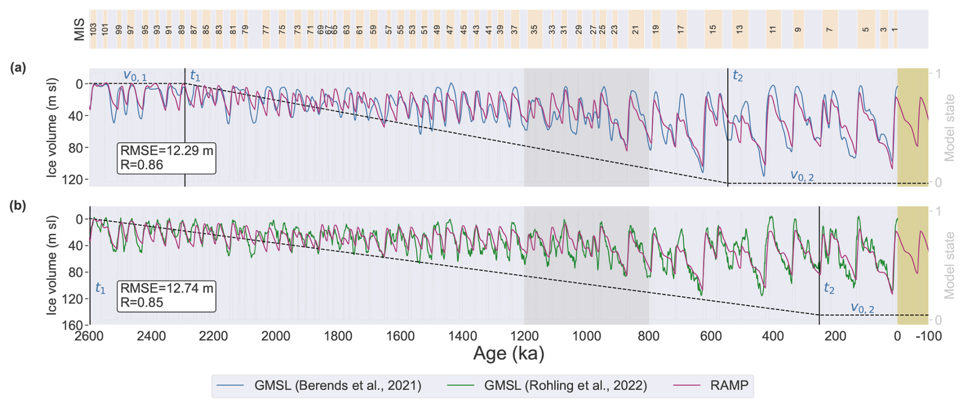
Figure 1 The RAMP model (purple lines) tuned for the two different tuning targets: (a) Berends et al. (2021a) GMSL curve and (b) Rohling et al. (2022) GMSL curve. The vertical black lines indicate the start and endpoint of the ramp and the dotted black lines show the temporal evolution of the deglaciation threshold. The grey-shaded area highlights the classical perspective of where the MPT is located in time. MIS boundaries are given according to Lisiecki and Raymo (2005). Simulations of the future 100 kyr are indicated by the yellow-shaded areas.

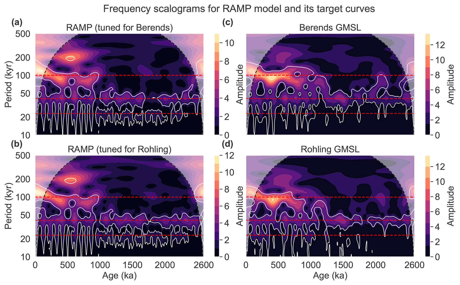
Figure 2 Frequency scalograms from the continuous wavelet transform for the RAMP model (a, b) and its corresponding tuning targets: (c) Berends et al. (2021a) GMSL curve and (d) Rohling et al. (2022) GMSL curve. White contours denote significant regions above the red-noise (AR1) background at the 95 % confidence level. Orbital frequencies of precession (∼ 23 kyr), obliquity (∼ 41 kyr) and eccentricity (∼ 100 kyr) are marked by the red dotted lines.

Simulating the future 100 kyr in the RAMP model yields consistent results for both curves. The next glaciation threshold is crossed for both curves 6 ka and the subsequent glacial cycle reaches its maximum at 64 kyr in the future. The RAMP model underestimates the Holocene minimum in global ice volume for both curves and projects an intermediate, strong future glaciation, compared to the previous glacial cycles.

The extended simulation period and the different tuning targets prevent a direct comparison between the RAMP and the L23 models. Hence, we run the RAMP model for a reduced simulation period of 2 Myr and tune it to the Berends GMSL curve. A comparison with the GRAD model, which is the best-performing model version of L23, demonstrates better model-data agreement with a reduction in RMSE of more than 1 m, while relying on three parameters less, but still providing more information on the temporal change in v₀(t). A complete comparison with all L23 model versions and the new RAMP model is shown in the Supplement (Fig. S1, Table S2).

3.2 Orbital forcing in the RAMP model

The temporal evolution of the global ice volume v(t) in the RAMP model is externally driven by the orbital forcing I(t). It is based on a linear combination of the precession parameter and obliquity (Eq. 3). The two associated tunable model weights α_Esi and α_O determine how the orbital forcing in the RAMP model looks and how strong the precession and obliquity signals are. Figure 3 shows the resulting orbital forcings for the RAMP model, when tuned for each of the two tuning targets. To identify the insolation curve corresponding to the obtained I(t) curve, we compare it to daily insolation curves at specific latitudes, monthly averaged ones, and various integrated summer insolations (ISI)¹. The insolation values are taken from La2004 orbital solution (Laskar et al., 2004). Insolation curves and orbital forcing in the RAMP model are normalized for comparison.

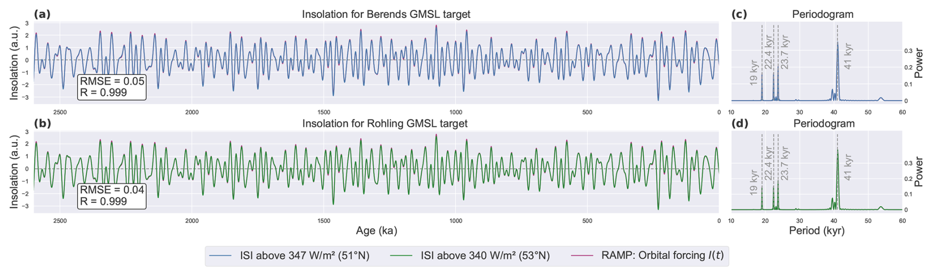
Figure 3 Comparison of the orbital forcing in the RAMP model (purple line), when tuned for the (a) Berends et al. (2021a) GMSL reconstruction, or the (b) Rohling et al. (2022) GMSL reconstruction. For each forcing curve, the best-fitting insolation curve is shown. ISI curves were calculated by code from Leloup and Paillard (2022). Panels (c) and (d) show the corresponding periodograms of both forcing curves.

The tuned weights (α_Esi, α_O) for the orbital forcing in the RAMP model exhibit large similarity for both targets (Table S3). Consequently, it is unsurprising that the obtained orbital forcings for these targets closely resemble one another, leading to a similar identification of the insolation curves with the highest correlation (Fig. 3a, b). For the Berends GMSL target, the closest correlation (R = 0.999) is found with the ISI above a threshold of 347 W m⁻² at 51° N, and for the Rohling GMSL target, the closest correlation (R = 0.999) is found with the ISI above a threshold of 340 W m⁻² at 53° N. The spectral analysis (Fig. 3c, d) of these insolation curves demonstrates that they consist of a dominant obliquity peak around 41 kyr, accompanied by pronounced precession peaks occurring around 19, 22.4, and 23.7 kyr.

3.3 Model sensitivity

We conduct several experiments to assess the sensitivity of the RAMP model to initial conditions, the robustness of the glacial patterns to changes in model parameters and simulation time and how robust the model tuning is. Since both GMSL targets result in very similar outputs, we investigate the model sensitivity for the RAMP model when tuned for the Berends GMSL. We use the optimal parameter set (Table S3) for the RAMP model, keeping all parameters fixed except one. The first parameter that we vary, v_i, sets the initial ice volume for v(t) (Fig. 4a). Lower initial values of 0 %, 50 %, 90 % and 95 % of the optimal value converge to the same output in less than 200 kyr. Similarly, higher values of 105 %, 110 %, 200 % and 1000 % converge to the same output in less than 200 kyr. This demonstrates that the RAMP model is not sensitive to the choice of initial ice volume.

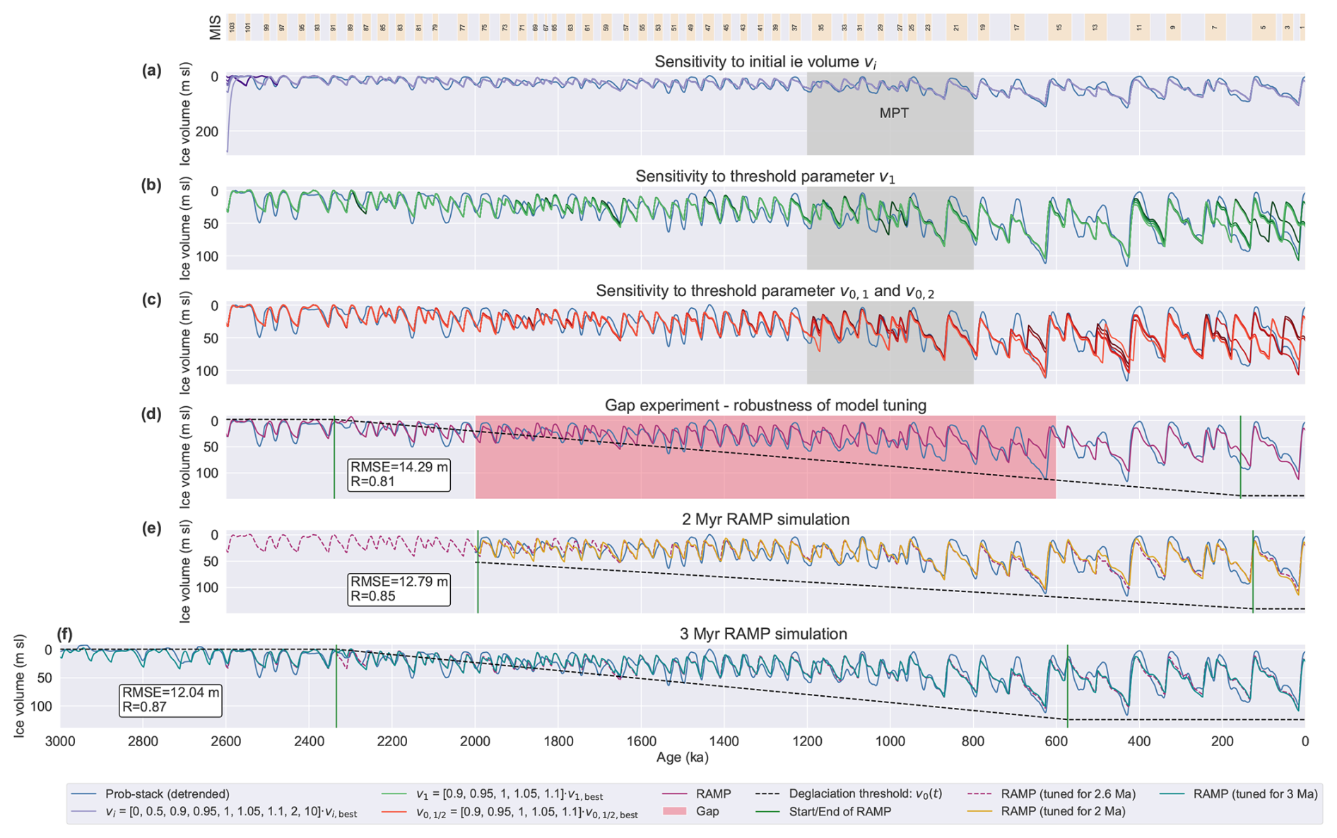
Figure 4 Parameter sensitivity in the RAMP model. (a) Sensitivity to initial ice volume: v_i is varied within $[\mathrm{0},\mathrm{0.5},\mathrm{0.9},\mathrm{0.95},\mathrm{1},\mathrm{1.05},\mathrm{1.1},\mathrm{2},\mathrm{10}]\cdot v_{i,\mathrm{best}}$ (purple lines). (b) Sensitivity to model threshold: v₁ is varied within $[\mathrm{0.9},\mathrm{0.95},\mathrm{1},\mathrm{1.05},\mathrm{1.1}]\cdot v_{\mathrm{1},\mathrm{best}}$ (green lines). (c) Sensitivity to model thresholds: v_0,1 and v_0,2 are simultaneously varied within $[\mathrm{0.9},\mathrm{0.95},\mathrm{1},\mathrm{1.05},\mathrm{1.1}]\cdot v_{\mathrm{0},\mathrm{1}/\mathrm{2},\mathrm{best}}$ (red lines). (d) Robustness of the model tuning. The RAMP model (purple line) was tuned for the Berends GMSL, starting from a unit vector and excluding the period 2–0.6 Ma (red-shaded area) from the tuning target. (e) RAMP model when tuned for a 2 Myr run (golden line) compared to the standard 2.6 Myr tuned version (purple dotted line). (f) RAMP model when tuned for a 3 Myr run (cyan line) compared to the standard 2.6 Myr tuned version (purple dotted line). The blue line shows the Berends GMSL. The grey-shaded area highlights the classical perspective of where the MPT is located in time. MIS boundaries are given according to Lisiecki and Raymo (2005).

The second parameter that we vary is the model threshold v₁, which we alter in an interval of ±10 % ($[\mathrm{0.9},\mathrm{0.95},\mathrm{1},\mathrm{1.05},\mathrm{1.1}]\cdot v_{\mathrm{1},\mathrm{best}}$) (Fig. 4b). There is almost no change in the simulated glacial cycles prior to the MPT. During the MPT, MIS 28 and 29 are affected by the altered model threshold. After the MPT, the interglacial double peak during MIS 7 seems to be most sensitive to this parameter change, and failing to detect this accurately can lead to an error propagation and an early termination of the last glacial period.

The last sensitivity test we perform concerns the deglaciation threshold v₀(t). Here, we simultaneously vary v_0,1 and v_0,2 in an interval of ±10 % ($[\mathrm{0.9},\mathrm{0.95},\mathrm{1},\mathrm{1.05},\mathrm{1.1}]\cdot v_{\mathrm{0},\mathrm{1}/\mathrm{2},\mathrm{best}}$) (Fig. 4c). This produces similar results as for the sensitivity test of v₁, although the model results are more sensitive to changes in v₀(t) than to changes in v₁. Pre-MPT cycles are almost not affected by these changes. During the MPT, MIS 29 and 30 are again affected, as well as MIS 35. Glacial cycles after the MPT are most sensitive to parameter changes. Simulating the interglacial double peak during MIS 7 is again problematic. Furthermore, MIS 17 and MIS 13 are sensitive to changes in v₀(t).

To assess the robustness of the model tuning, the RAMP model is tuned from a unit vector (i.e. initial parameter guess of 1 for all parameters) to the Berends GMSL curve, excluding the time interval from 2 to 0.6 Ma from the target dataset. Consequently, the RAMP model is only tuned for the early Quaternary (2.6–2 Ma) and the late Quaternary (last 600 ka), without any information on the glacial cycles during the gap period. The reconstructed global ice volume closely aligns with the Berends curve (Fig. 4d). In comparison with the reconstructed curve tuned to the complete target (Fig. 1a), the exclusion of the gap results in a slight reduction of the R value from 0.86 to 0.81. The indicated ramp period remains extended with a similar start point at 2339 ka (previously 2291 ka), but a later end at 157 ka (previously 546 ka). Despite lacking any information on the glacial cycles during the gap period (red-shaded area in Fig. 4d), the RAMP model can accurately reconstruct the timings of most glacial terminations. Excluding MIS 16 from the tuning target (it falls within the gap period) leads to a failure in reconstructing its large ice volume extent in the RAMP model. Instead, the first extended ice sheets occur later in the simulation, which is linked to the later endpoint of the ramp. Despite MIS 16, the RAMP model is demonstrating high robustness of the applied model tuning with no signs of overfitting. The strong performance of the RAMP model in reliably reproducing glacial cycles, despite lacking any prior information about them, is demonstrated by the high correlation (R = 0.81) between the gap-tuned RAMP model and the Berends curve.

Finally, we alter the simulation period to verify the robustness of the glacial patterns and whether the identified ramp period changes. When we tune the RAMP model for a reduced period of 2 Myr to the Berends GMSL and compare it with the 2.6 Myr tuned version of the RAMP model, both curves almost perfectly align for the past 2 Myr (Fig. 4e). The end of the ramp occurs later in the Quaternary at 127 ka (previously 546 ka). The onset of the ramp is bounded to 2 Ma, due to the reduced simulation period. However, the optimal value for the onset lies very close to this upper bound at 1993 ka, indicating that t₁ might exceed this upper bound, as it does for the 2.6 Myr run.

We repeat the same experiment, but for an extended simulation period of 3 Myr (Fig. 4f). Over the past 2.6 Myr, both curves align almost perfectly. Without an upper bound of 2 Ma for t₁, as in the previous simulation, the model tuning finds a very similar pattern for the temporal shape of the ramp for the 3 Myr run and the 2.6 Myr run. The 3 Myr run results in an onset of the ramp at around 2334 ka (previously 2291 ka) and an end at 573 ka (previously 546 ka). Hence, altering the simulation period for the RAMP model does not largely affect the simulated glacial patterns, and the long-lasting trend obtained for the ramp is a robust feature for all simulation periods, although the exact duration of the ramp may vary between the simulations.

4 Discussion

4.1 Ramp-like change in the deglaciation parameter

Conceptual models like the RAMP model cannot shed light on the underlying physical mechanisms directly (e.g. whether a long-term trend in v₀ is due to regolith removal or a gradual CO₂ decrease), since they do not include the involved physical or chemical processes directly. However, their strength lies in their capability to investigate the underlying temporal structure of such a change. The advantage of the new ramp formulation is that the RAMP model incorporates multiple scenarios for the temporal change in the deglaciation parameter, particularly all those discussed in Legrain et al. (2023) (ORB, ABR, GRAD). By tuning the model to a GMSL target curve, it selects the most appropriate temporal structure for v₀(t) to reconstruct this curve.

In this study, we applied the new RAMP model to two different GMSL curves. Both targets led to a similar pattern, namely a long-lasting increasing trend in v₀(t), which started between 2.6 and 2.3 Ma and ended between 550 and 250 ka. Hence, for these targets, the RAMP is not in favour of an abrupt change, a rather short and limited change (e.g. which only lasted during the MPT) or no change in v₀(t), which would correspond to a purely orbitally driven climate. These findings agree with the results of the L23 models, where the authors identified a gradual trend over the entire 2 Myr-long simulation period to be more likely than an abrupt one or a purely orbital one. The strength of the RAMP model is that it gives information about a potential start and end of such a gradual change. The L23 GRAD model was only run for the past 2 Ma, therefore, it does not allow earlier changes in v₀, but the RAMP model reveals that the change in v₀ likely started even before 2 Ma. An alternative approach is presented in Ganopolski (2024), where the author prescribes the change in the critical ice volume parameter v_c (similar to our v₀) with a hyperbolic tangent, which closely resembles the temporal evolution of the regolith-free area as described in Willeit et al. (2019). This shows that the regolith-free scenario can reproduce the MPT, but since it relies on a single prescribed temporal structure for this change in v_c, it gives no information on how likely such a temporal structure is.

The RAMP model challenges the possibility that orbital forcing alone could explain the MPT. Despite the flexibility of using different linear combinations of the precession parameter and obliquity (even when including co-precession), tuning the RAMP model did not result in a scenario where v₀(t) remained constant, but always increased over the Quaternary, i.e. implying that an internal change in the system is required to reconstruct the MPT. In contrast, there are recent studies linking the occurrence of the MPT to orbital forcing alone. Ma et al. (2024) introduce the integral of annual mean insolation anomaly (IAMIA), which quantifies successive small step-wise insolation changes over a given period of time. The authors show that IAMIA exhibits a large shift around 935 ka, which they hypothesise to have enabled the onset of the MPT. Another recent study by Verbitsky and Omta (2026) discusses the idea that the MPT is due to a delayed relaxation process, which can lead to an abrupt-like jump in the dominant period. This shift in periodicity can be highly sensitive to the initial conditions, and the sensitivity depends on the amplitude of the orbital forcing. Although our model yields a contrasting view, we cannot exclude the possibility that a different orbital parameterization, e.g. IAMIA, could recreate the MPT.

While the RAMP model supports a long-lasting gradual trend in the Earth-climate system, its underlying physical mechanism cannot be directly inferred but just hypothesized since the conceptual modelling approach lacks the physical representation of these mechanisms. Whether a gradual erosion of regolith (Clark and Pollard, 1998; Clark et al., 2006), a gradual decrease in atmospheric CO₂ (Berends et al., 2021b; Scherrenberg et al., 2025), some sea-ice feedback mechanism, a mixture of these (Willeit et al., 2019) or something else, is the underlying mechanism behind this trend, requires a more physics-based model which can explicitly resolve these mechanisms.

As Verbitsky and Crucifix (2023) point out, while some phenomenological models can very accurately recreate some climatic time series, it does not necessarily reflect their physical similarity to nature. Hence, it is crucial to investigate whether such a ramp-like scenario in the model is justified by paleo records or more sophisticated modelling studies. A synthesis of globally distributed sea surface temperature (SST) records by Clark et al. (2024) found that two long-term cooling stages occurred during the last 4.5 Ma. The first started around 4 Ma, which was followed by a second period of intensified cooling between 1.5 Ma and around 0.8 Ma. Thereafter, temperatures stabilised for the late Pleistocene. A statistical model by Tzedakis et al. (2017) relates glacial terminations with a required energy threshold and shows that this deglaciation threshold had to rise over the Pleistocene. They found that the increase is ramp-like with a linear trend lasting from 1.55 Ma until 0.61 Ma. The conceptual model by Ganopolski (2024) can also recreate the MPT by changing its critical ice volume parameter ramp-like rather than linear. However, it uses a smoother transition function, namely a hyperbolic tangent centered around 1050 ka with a transition time of 250 kyr. The asymptotic behaviour of the hyperbolic tangent leads to quasi-constant parameter values prior to 1.55 Ma (twice the transition time) and after 0.55 Ma. The author stresses the similarity with the modelled regolith mask in Willeit et al. (2019), connecting the ramp-like structure with the erosion of the Northern Hemisphere regolith. The optimal volcanic CO₂ outgassing scenario (V2) found in Willeit et al. (2019) resembles a ramp-like structure for the past 2.6 Ma with a decreasing trend of volcanic CO₂ outgassing between around 2.1 and 0.9 Ma.

In summary, certain proxy records and modelling studies support the concept of a ramp-like internal change. Reaching a constant value for v₀(t) in the RAMP model, after a long increasing trend, aligns with findings from SST records (∼ 0.8 Ma, Clark et al., 2024), a statistical model of energy thresholds (∼ 0.6 Ma, Tzedakis et al., 2017) and with a modelled volcanic CO₂ outgasing scenario (∼0.9 Ma, Willeit et al., 2019), where stable conditions were reached in the late Quaternary, although the endpoint for the RAMP model (0.25–0.55 Ma) occurs later. The volcanic CO₂ outgassing scenario in Willeit et al. (2019) closely resembles the temporal structure in the RAMP model with an early onset around 2.1 Ma. On the other hand, the first cooling trend in global SST records appears earlier (4 Ma), and the intensified cooling trend around 1.5 Ma appears later than the one in the RAMP model. Moreover, the ramp-like energy threshold in Tzedakis et al. (2017) also suggests a later start around 1.55 Ma.

4.2 Simulation of the next glacial cycle

While neglected in many conceptual models, simulating the next glacial cycle can be an important tool of model evaluation, since this represents the only time interval in which a model cannot be tuned or fitted onto some existing paleoclimatic target curve and it can reveal model deficiencies. Since the simulated curves lack anthropogenic CO₂ emissions, they must be interpreted as baseline experiments of how the glacial cycles would evolve in the absence of anthropogenic impacts. The RAMP model consistently crosses the next glaciation threshold 6 ka, lasting until 64 kyr in the future. Some other conceptual models also simualted the next glacial cycle: Calder (1974) projected the next glacial onset 5 ka, lasting until around 119 kyr (see his Fig. 2), Imbrie and Imbrie (1980) estimated a start 6 ka (see their Fig. 7) and Fig. 5 in Paillard (2015) reveals that only a large enough glaciation threshold can lead to a prolonged Holocene in the P98 model, while a lower threshold would have terminated the Holocene already a few kyr ago. While other models like the L23 models and the Leloup and Paillard (2022) model were not simulating future cycles, it can be expected that they would yield similar results as the RAMP model (i.e. a short Holocene), since they are based on similar model dynamics. In their recent study, investigating the influence of precession and obliquity on glacial interglacial cycles, Barker et al. (2025) estimate that the current interglacial conditions would last for 11 kyr, when obliquity reaches its next minimum and the succeeding glacial would be interrupted in around 66 kyr (again neglecting anthropogenic effects).

These results do not agree with more complex models, coupled to the carbon cycle, which project, even without any anthropogenic influence, an unprecedentedly long Holocene, lasting for another 50 kyr (Ganopolski et al., 2016; Talento and Ganopolski, 2021). Hence, the short Holocene, the crossing of the next glacial threshold 6 ka and the failure in stimulating the Holocene minimum in global ice volume do not align with these more complex models. These deficiencies stem from the model design, which does not recognize interglacial states as stable states in the model and yields quick deglaciations followed by long-lasting glaciations. This becomes apparent from the model equations: in the late Pleistocene, when large ice volume is present, the term $\frac{v\left(t\right)}{{\mathit{\tau }}_{\mathrm{d}}}$ (Eq. 5) dominates the deglaciation regime and leads to very quick removal of the large ice sheets. Hence, the next glaciation threshold $v\left(t\right)\cdot \stackrel{\mathrm{̃}}{I}\left(t\right)<v_{\mathrm{1}}$ (Eq. 7) is rapidly crossed in the model, leading to a short interglacial state, which is immediately followed by an increase in global ice volume (Eq. 4). Hence, by its very design, the RAMP model cannot produce extended interglacial states and will instead rapidly transition to the next glaciation. This model limitation could be addressed in a future study, either by modifying the threshold equations or by adjusting the differential equation in the deglaciation regime in such a way that it also allows for stable interglacial conditions, instead of just for rapid ice loss.

4.3 Role of precession and obliquity

While we cannot directly investigate the physical effects of precession and obliquity in the climate system with the RAMP model, we can investigate their influence on the dynamics of the model. By using a linear combination of the precession parameter and obliquity rather than a single insolation metric, we can explicitly see which roles these two functions of orbital parameters play in the model. For instance, this allows us to investigate the spectral power of the obtained orbital forcing in the RAMP model.

The evolution of the global ice volume v(t) in the RAMP model is driven by a linear combination of the precession parameter and obliquity, weighted by the model parameters α_Esi and α_O. Therefore, the orbital forcing in the model depends on the tuned values of these two parameters. Compared to other conceptual models, which rely on a specific insolation metric for the orbital forcing (e.g. Ganopolski, 2024; Paillard, 1998; Leloup and Paillard, 2022), this allows for more flexibility in the model and reduces subjective modelling choices. A similar approach with three functions of orbital parameters has been successfully used in other models (Imbrie et al., 2011; Legrain et al., 2023). Choosing a specific insolation metric does affect the quality of the reconstruction result due to variations in their spectral profiles (Leloup and Paillard, 2022). For instance, the insolation at summer solstice at 65° N has a stronger precession signal than the one obtained from the caloric summer half-year insolation at 65° N (as introduced by Milankovitch, 1941).

Moreover, since using a linear combination of the precession parameter and obliquity can accurately reconstruct various insolation curves at different latitudes and seasons (Sect. S4), the tuning process will select an optimal curve for the orbital forcing. This optimal forcing curve can then be compared to real insolation curves. In addition, available conceptual models use a variety of orbital forcings, e.g. Model 3 (Ganopolski, 2024) uses the maximum summer insolation at 65° N, P98 relies on the same metric, but with an artificial truncation function added, Tzedakis et al. (2017) use the caloric summer half-year insolation at 65° N. Regarding this variety of different orbital forcings in use, it is of interest to see which metric the RAMP model selects. For the RAMP model, we find that the tuned orbital weights (α_Esi, α_O) are almost the same for both target curves and hence are the orbital forcings I(t). We find that the curve with the highest correlation (R = 0.999) is the ISI above a threshold of 347 W m⁻² at 51° N for the Berends curve and the ISI above a threshold of 340 W m⁻² at 53° N for the Rohling curve. These curves consist of a dominant obliquity peak and substantial precessional signals. This contrasts with the widely used insolation curve at summer solstice at 65° N, which exhibits dominant precession signals and a reduced obliquity signal. However, it therefore better resembles the precession-obliquity imprint of the caloric summer half-year insolation curve.

4.4 Model limitations

The RAMP model depends on a specific threshold choice to switch between a glaciation and a deglaciation state. Köhler and van de Wal (2020) challenge this binary view of interglacials and glacials. By classifying interglacials based on the absence of substantial NH land ice outside of Greenland, they found that the classification of interglacials, especially in the early Quaternary, is ambiguous. This classification depends on the defined threshold and the choice of the underlying target curve. This perspective questions the ability of any threshold-based, two-state model to unambiguously classify interglacial states. Therefore, the identified glacial and deglacial states in our model should only be carefully considered in combination with the applied thresholds, defined in Eqs. (6), (7), and for the used target curve.

Available global mean sea level reconstructions exhibit large uncertainties. Between 50 and 30 ka, geological and geochemical reconstructions of GMSL vary up to 60 m and above (Farmer et al., 2023). Model-based deconvolutions of global δ¹⁸O into GMSL, like for the Berends et al. (2021a) and Rohling et al. (2022) sea level reconstructions, exhibit similar large uncertainties. While the Berends curve shows a Last Glacial Maximum (LGM) lowstand of around 100 m, the Rohling curve gives around 108 m. Both values are well below observational-based reconstructions of around 130–135 m for the LGM (Austermann et al., 2013; Lambeck et al., 2014; Yokoyama et al., 2000). Furthermore, the Berends and Rohling reconstructions, although differing in their modelling approaches, both rely on the LR04 benthic δ¹⁸O stack, whose age model was orbitally tuned. Hence, the chosen reconstruction depends on the orbital tuning applied to the LR04 stack. Consequently, the simulated global ice volume in the RAMP model has to be interpreted in light of the large uncertainties already present in the target data.

Our findings are constrained not only by the uncertainties in the Berends and Rohling GMSL reconstructions but also by the specific choice of which GMSL curve to use as the target for our model. On the one hand, GMSL reconstructions (and hence global ice volume), as the ones of Berends et al. (2021a) or Rohling et al. (2022), exhibit small global ice volume during the early Pleistocene, followed by an increase in amplitude and frequency after the MPT. On the other side, the new GMSL curve by Clark et al. (2025a) differs fundamentally from former GMSL reconstructions by no longer exhibiting an increase in ice volume over the Pleistocene, but just a shift in glacial frequency. This leaves us with two contrasting views on the evolution of the global ice volume over the MPT. In this study, we selected the Berends and Rohling GMSL curves as target curves instead of the newly published Clark GMSL. This has the following reason: the RAMP model is based on former models (P98, L23), which were specifically designed to simulate an increase in ice volume through an increasing v₀ parameter, hence, the RAMP model is adapted to reconstruct GMSL curves which do show an increasing trend in global ice volume. So, by its model design, the RAMP model is not suited for a GMSL curve as the one presented by Clark et al. (2025a), since this data set no longer exhibits an increase in ice volume. However, we tested various approaches to adjust the RAMP model to simultaneously reconstruct the structurally different Berends and Clark GMSL curves. It seems that an adjustment of the glaciation threshold in combination with a ramp-like change in these threshold parameters is needed. We present this adjusted model, which we call RAMP-2, in the Supplement (Sect. S7). However, further tests are needed to verify the performance of the RAMP-2 model. Thus, leaving us with the RAMP model, applied to the Berends and Rohling GMSL reconstructions. Since the RAMP model is only applicable to a subset of the available GMSL curves, namely the ones which do show an increase in global ice volume, our finding that a long-lasting trend in the deglaciation parameter is key in reproducing the MPT, is limited to these types of GMSL curves and this specific interpretation of the MPT.

5 Conclusions and outlook

In this study, we constructed a new conceptual model of the Quaternary global ice volume, the so-called RAMP model. It improves the previous L23 models of Legrain et al. (2023) by reducing the model-data mismatch (ΔRMSE > 1 m), increasing the numerical efficiency (speedup of ∼ 30), refining the tuning strategy, simulating the next glacial cycle in the model, testing the model on another target curve, and implementing a more flexible ramp-like parameterization, which includes all former L23 temporal scenarios. Meanwhile, the required number of model parameters has been reduced by two to four. The model is insensitive to its initial conditions, i.e. the initial ice volume v_i. While the early Quaternary cycles are less sensitive to changes in the threshold parameters ($v_{\mathrm{0},\mathrm{1}/\mathrm{2}}$, v₁), the late Quaternary ones are more sensitive, particularly the appearance of interglacial double peaks around MIS 13 and MIS 7. The model tuning is very robust and can yield consistently good results, even when large parts of the tuning targets are excluded, indicating no signs of overfitting. Reducing or extending the simulation period does not largely affect the simulated glacial cycles, and the identified long-term change in the deglaciation parameter is a very robust feature in the model, although the timing for the onset and end of the ramp varies.

The RAMP model yields consistent results for both tested GMSL curves (Berends and Rohling). Both result in a long-lasting increasing trend in the deglaciation parameter v₀, which started in the early Quaternary (2.6–2.3 Ma) and lasted until 550–250 ka, in order to reconstruct the MPT. The RAMP model consistently projects a short Holocene by crossing the next glaciation threshold 6 ka, followed by an intermediate strong glacial, lasting until around 64 kyr in the future. However, it underestimates the Holocene minimum in global ice volume.

Furthermore, the RAMP model selects a very similar orbital forcing curve for both GMSL targets, which is in close agreement with the ISI above a threshold of 347 W m⁻² at 51° N for the Berends curve and the ISI above a threshold of 340 W m⁻² at 53° N for the Rohling curve. Both curves are characterised by a dominant obliquity peak and substantial precession signals. This pattern more closely matches the caloric summer half-year insolation than the insolation at summer solstice at 65° N.

The RAMP model uses only the precession parameter and obliquity as inputs, along with a time-dependent v₀ parameter, to reconstruct global ice volume throughout the Quaternary. Internal feedback mechanisms and forcings are conceptualized by aggregated model parameters. The early onset of the ramp-like change emphasizes the importance of intensifying the work to obtain an even older continuous ice core record than the recently drilled at least ∼ 1.2 Ma old ice from the European Beyond EPICA-Oldest Ice Core project to shed further light on the MPT.