
the Creative Commons Attribution 4.0 License.
the Creative Commons Attribution 4.0 License.
 | 20 Nov 2026
How abruptly did the Holocene Green Sahara end?
Martin Claussen

Anne Dallmeyer
Frank Darius
Philipp Hoelzmann
Michèle Dinies
Discussion about abrupt changes in the Sahara at the end of the African Holocene Humid Period has generally remained qualitative. Here we move the long-standing debate to a quantitative, metric-driven assessment, and we provide a rigorous framework to characterize abruptness of vegetation changes in a transient simulation of the MPI (Max Planck Institute) Earth System model and proxy records (dust flux and pollen data) for the last 8000 years. In the simulations, we find the strongest long-term increase in simulated bare surface in a north-west to south-east oriented strip of some 400 to 800 km in north-south direction between approximately 20° N in the west and 15° N in the east. Grid boxes in this region reveal abrupt, step-like transitions with changes in simulated bare surface, or conversely, in the total vegetation cover, which occur on average some 4 times faster than the approximately linear trend in the orbital forcing. The transitions in simulated grass and tropical tree plant functional types, i.e., in the type of the vegetation cover, appear to be up to twice as abrupt and up to twice as fast as the transition in the total vegetation cover. The reconstructed dust flux into the Atlantic shelf area at around 20° N, which we interpret as spatially aggregated changes in the openness of the landscape in the western Sahara, reveal a step-like transition with a much stronger abruptness than the simulated transition in bare surface in this region. The pollen records, however, indicate a rather gradual increase in desert-like conditions (with only one exception), but in many records, abrupt and fast transitions in Guinean, Sudanian and Sahelian phytogeographical groups occur. Hence our standardized, metric-driven analysis of model and data suggests that vegetation composition in the Holocene Sahara can undergo substantially more abrupt transitions than total vegetation cover, and that a gradual expansion of desert areas on a large scale can be accompanied by abrupt, step-like transitions within local ecosystems.
- Article
(13516 KB) - Full-text XML
- BibTeX
- EndNote


The multiple witnesses documenting a Sahara greener than today during the time period between approximately 11 500 to 4500 years ago (e.g., Hély et al., 2014; Kuper and Kröpelin, 2006), continue to attract attention to this day, as it contrasts sharply with today's largest hot desert environment. Subtle, millennial-scale variations in the Earth's orbit caused changes in the seasonal distribution of insolation which triggered the transitions from wet to drier conditions during the mid-Holocene, between 8200 to 4200 years ago. The resultant changes in climate and ecosystems, however, can only be explained when taking into account the feedbacks between the atmosphere, the ocean and mainly the land surface with its soils, vegetation and lakes as amplifier (e.g., Claussen et al., 2017; Pausata et al., 2020).
Based on theory and climate modeling (Brovkin et al., 1998; Claussen et al., 1999) an abrupt termination of the “Green Sahara” – a term coined by L.E. Almásy in 1934 (Almásy, 1997) – was postulated. Reconstructions of dust deposition in marine sediment records off the West African coast (deMenocal et al., 2000; McGee et al., 2013) and deuterium values from the Horn of Africa region (Tierney and deMenocal, 2013) and Western Africa (Tierney et al., 2017) seemed to support the early modeling studies. In contrast, analyses of pollen and sediment laminations in the Central Sahara and its southern fringes (Francus et al., 2013; Kröpelin et al., 2008; Lézine et al., 2011; Salzmann and Waller, 1998; Waller et al., 2007) indicated a gradual transition of ecosystems. A synthesis of hydrologic reconstructions across Africa (Shanahan et al., 2015) based on different proxies (e.g. arboreal pollen, pollen concentrations and diatom ratios) showed that the termination of the humid condition in Northern Africa was only locally abrupt, dynamics also seen in at least one state-of-the-art climate system model (Dallmeyer et al., 2020). Recently, it was supposed that most climate system models are tuned to stability, but if a model is optimized to reproduce a Green Sahara, then it also displays threshold behavior (Hopcroft and Valdes, 2021).
So far, the discussion of the abrupt termination of humid conditions and associated vegetation changes in the Sahara had developed in a rather qualitative way, although the question of how rapidly vegetation spread throughout the Sahara during mid-Holocene is an important issue as it presumably affected the time frame for human adaptation. Only few attempts have been made to standardize the degree of abruptness. Brovkin et al. (2021) gave an overview of past abrupt changes, tipping points and cascading impacts on ecological and societal systems. They referred to abrupt changes as changes faster than the relevant forcing, i.e., the variations in the Earth's orbit in the paleoclimate context. Trauth et al. (2018) introduced a formal detection of abrupt changes in paleo records by using a changepoint analysis. Dallmeyer et al. (2021) analyzed global climate-vegetation simulations of the last 8000 years and quantified the rapidity of simulated vegetation changes in terms of the strongest slope that emerges in the vegetation time series.
Here, we aim at developing a standardized, metric-driven approach to provide a quantitative framework for consistently comparing abrupt transitions in paleoclimate simulations and paleodata. Our approach is guided by the earlier studies: We search for abrupt, step-like transitions by computing changepoints in linear regression (Trauth et al., 2018) in the vegetation time series, and we calculate the offset at the changepoints relative to the variability in the data as suggested by the edge detection of Bathiany et al. (2020). Thereby, we are able to specify the degree of abruptness and to differentiate between more or less abrupt and gradual changes. In addition, we compute the slope of the data series at the changepoint to provide estimates on how much faster an abrupt transition occurs relative to a change in the approximately linear insolation forcing due to multimillennial variations in the Earth's orbit.
However, developing a metric to answer the question of how abruptly the Green Sahara ended is just a first step. The second challenge concerns the characterization of the Green Sahara, i.e. the vegetation in the Holocene Sahara, in data and models. To trace the history of the Holocene greening and aridification of the Sahara different proxies have been investigated and explored such as lake level fluctuations and occurrences of lakes and wetlands (Hoelzmann et al., 2004; Holmes and Hoelzmann, 2017; Lézine et al., 2011) or geochemical proxies such as plant waxes and/or their isotopic composition (Eglinton et al., 2002). To avoid comparison of various proxies with differing sensitivities to climate and to enable a more direct comparison between data and simulation of Saharan greening, we explore the use of vegetation proxies, such as fossil pollen spectra aggregated into phytogeographical groups, and clusters of simulated plant functional types, complemented by reconstructions of the deposition of Saharan dust into the North Atlantic as a proxy of the openness of the western Sahara landscape (see Egerer et al., 2016, 2018).
We therefore organize our paper as follows. Section 2 presents data and methods: representation of North African vegetation in the Max Planck Institute Earth System Model (MPI-ESM) (Sect. 2.1), palynological data from continental sites including the aggregation of individual pollen taxa into pollen groups (Sect. 2.2), comparison of simulated PFTs and pollen data (Sect. 2.3), dust deposition time series from marine sediments cores (Sect. 2.4), and the development of the new metric for quantifying abruptness and rapidity (Sect. 2.5). In Sect. 3, we first present our results: the patterns of long-term tendencies, abruptness and rapidity (Sect. 3.1) with a focus on regions and individual pollen records (Sect. 3.2). We then discuss how the timing of abrupt changes identified in data and simulation relates to the termination of the African Holocene Humid Period (AHHP) (Sect. 3.3), and we explore the question of whether the abrupt vegetation changes found in our simulation are associated with abrupt changes in precipitation, the main climatic driver of vegetation changes in the Sahara (Sect. 3.4). We discuss limitations and challenges of our analysis in Sect. 4, and we end with a conclusion in Sect. 5.
2.1 Simulated plant functional types
We analyze the transient Holocene simulation presented in Dallmeyer et al. (2021) that was done using the MPI-ESM1.2 (Mauritsen et al., 2019) at a spectral resolution of T63 (approx. 200 km on a Gaussian grid) for the atmosphere and the land. The simulation starts at 6000 BCE, corresponding to approximately 7.95 ka BP, and ends in 1850 CE, corresponding to 0.1 ka BP. In the following, ages are reported in ka BP (in short: ka), with BP referring to years before 1950 CE. The transient simulation reproduces the global patterns of Holocene vegetation transitions (Dallmeyer et al., 2021). A similar simulation from the same ensemble of MPI-ESM Holocene simulations, but with slightly different boundary conditions, demonstrates that the MPI-ESM Holocene simulations also capture the reconstructed time-transgressive termination of the AHHP (Dallmeyer et al., 2020).
For a detailed description of how the vegetation is computed in the land-surface model JSBACH of the MPI-ESM, we refer to Brovkin et al. (2009) and Reick et al. (2013, 2021). Here, we only mention the most important items relevant for our study. In JSBACH, each land grid cell in the land-surface model is partitioned into a fraction of bare surface fbare, unsuitable for vegetation growth, a fraction of natural vegetation fveg, represented by different plant functional types, and a fraction of anthropogenic land use flu. The cover fraction ranges from 0 to 1 such that . Land use is prescribed following the LUH2 land-use forcing by Hurtt et al. (2020). This forcing complies with the CMIP6 protocol, it is read annually, but is calculated daily by linear interpolation. The forcing begins 850 CE with a quasi-linear transition period of 1000 years starting 150 BCE to slowly build up the land use. In the simulations, land use only appears in a few grid boxes in the Niger delta and to the north of it up to some 12° N during the last 2000 years. Hence in the region of this study, holds for almost all grid boxes considered.
The computation of the bare surface fraction is based on the idea that a bare surface develops when the net-primary production (NPP) of plants gets too low so that vegetation is repeatedly not able to grow an extended canopy at least once during a year. Vegetation coverage is computed as function of the biomass that is allocated to leaves. To avoid unrealistic year-to-year fluctuations in bare surface fraction, a delayed development of bare surface is assumed with a time scale of 50 years. In reality, however, fluctuations between a sparse vegetation cover and the expansion of bare surface can happen on a seasonal time scale, especially in semi-desert and desert regions. Implicit in the implementation of such a time scale in our model is the assumption that in such a large area as a grid box, which amounts some 40 000 km2, expansion of bare surface does not occur all the sudden within a year. The time delay is also introduced to avoid annual flickering which would cause numerical problems, specifically regarding the simulated carbon fluxes.
Natural vegetation in the land-surface model JSBACH of the MPI-ESM is represented by eight different plant functional types (PFTs): Tropical or extratropical, evergreen or deciduous tree types, rain green or cold-resistant shrub types, and C3 and C4 grass. In theory, all PFTs can coexist in each terrestrial grid-cell. The occurrence of each PFT is limited by temperature constraints in the model. For the Sahara, the decisive bioclimatic limit is the cold resistance defined in terms of the mean temperature of the coldest month. In the northern hemisphere during the mid-Holocene boreal winter, insolation was weaker than today and, hence, the coldest month colder than today. The temperature of the coldest month is the limiting factor for tropical trees. There are no bioclimatic limits defined with respect to moisture requirements. These are implicitly included in the computation of NPP of each PFT which controls the competition between them.
The time scales of changes in the coverage proportions of PFTs is governed by the time scales implicit in the NPP dynamics of the competing PFTs. The time scales relevant for the present study range from 30 years for tropical trees, 12 years for rain green shrubs and 1 year for grass. If climate changes and if different PFTs can exist within the range of climate variability, then the PFT with the strongest NPP dominates, and the time scale of the transition mainly depends on the difference in the carbon allocation of the competing PFTs. If this difference is small, then the transition is slow. The fastest changes occur, if the climate crosses a bioclimatic threshold. When the temperature of the coldest month drops below 15 °C, for example, then the growth of tropical trees is set to zero in the model. The same happens, if strong wind or fire events occur in the simulated climate. Then, the tropical tree PFTs affected decay exponentially within a few decades. An overview of time series of bare surface fraction and relevant PFTs in the African and Arabian desert belt is given in the Appendix, Fig. A1.
2.2 Pollen data
We use the proven concept of phytogeographical regions to assess and visualize major vegetation changes documented by means of pollen analysis (e.g., Maley, 1973; Ritchie and Haynes, 1987; White, 1983). According to this concept, the various pollen types are assigned into four phytogeographical groups – Saharan, Sahelian, Sudanian and Guinean – according to the region in which they prevail in today's climate. Very briefly, the transition from the Mediterranean region to the Saharan region roughly coincides with the 100 mm isohyet (e.g., Le Houérou, 1990; Olson et al., 2001), while the southern border of the Sahara roughly coincides with the 150 mm isohyet (e.g., Quézel, 1965). The Sahelian climate is characterized by annual mean temperatures above 24 °C (Sayre et al., 2013), a long dry period, with most rainfall occurring during the three to four summer months ranging from 100–250 mm of rainfall per year and a very long dry season in the north to some 250–500 mm of rainfall in the south. In the Sudanian region, there are again distinct differences between humid and dry periods, with an annual rainfall of over 500 mm. In contrast, the Congo-Guinean equatorial region experiences very high levels of precipitation (over 3000 mm yr−1) and consistently high temperatures.
Different plants can also grow outside their main phytogeographical region in, for example, mountains or alongside (temporary) water courses, thus in habitats characterized by differing conditions than the main phytogeographical region. Yet the vegetation outside of these habitats aligns with the regional climate conditions (Walter and Breckle, 1991). This implies that with a changing climate, plants belonging to a phytogeographical group can migrate into regions previously not occupied by them.
The assignments of pollen types to phytogeographical groups applied here are based on the classifications by Vincens et al. (2007) and Hély et al. (2014) with some modifications. For the present study (for details see Dinies et al., 2026) we slightly changed the proportion computation: Rather than calculating the center-log values of the pollen counts, we computed the percentage values, with the sum of all terrestrial types, including grasses, equaling 100 %. These percentages were then multiplied by the phytogeographical proportion established for each pollen type. The proportions summed-up per sample of the four regions, Guinean, Sudanian, Sahelian and Saharan, i.e. the computed phytogeographical affinities of each sample, are shown. For the grasses, the percentage proportions of the sum of terrestrial types are plotted (after the square-root transformation of the counts).
In addition to the phytogeographical groups described, we implement grasses (Poaceae) as independent group. The pollen morphology of grasses does not allow a distinction between “Sahelian”, “Sudanian” or “Saharan” grasses. We thus consider them separately and explore the question of whether their trends follow any of the phytogeographical groups.
The pollen data are retrieved from the African Pollen Database compiled by Phelps et al. (2019). We consider all sites with more than ten samples and age depth models based on 14C dating, located in the investigated region of Northern Africa (see Dinies et al., 2026). We exclude the Mediterranean region and the East African Highlands due to their markedly different ecology, and we exclude pollen records which do not cover the last 8000 years. An overview of the time series of phytogeographical groups and Poaceae and their geographic location is provided in Figs. A1, A2, and Table A1.
2.3 Comparison of simulated PFTs and pollen data
PFTs in an Earth system model are designed to describe the interaction of vegetation and near-surface fluxes of energy, water, momentum and terrestrial carbon for all regions of the Earth rather than to realistically capture the large spectrum of plant functional diversity and landscape characteristics. In contrast, pollen types representing respective plant taxa often are a conglomerate of life forms (trees, shrubs, perennials, annuals), thus not directly equivalent to a PFT, even more so as we have merged the pollen types into phytogeographical groups to obtain a more standardized reference. Therefore, assignment of simulated PFTs to phytogeographical groups cannot be derived from first principles, but is based on conceptual, ad hoc considerations. Here we compare a) the bare surface fraction with the Saharan phytogeographical group, b) the sum of tropical tree PFTs with the Sudanian and the Guinean group, and c) the grass PFT with the Poaceae. In the following, we explain and discuss these assignments.
The taxa of the Saharan phytogeographical group stand for key features of every desert vegetation: plant coverage is extremely low and restricted to wadis, runnels, and bases of rocks, small depressions, and similar structures. These microstructures of the desert landscape are not represented by the coarse resolution of the topography in an Earth system model. But the Saharan plant taxa also are an indicator of the openness of the desert landscape, making a qualitative comparison with simulated bare-ground fraction appropriate. A direct quantitative comparison is not attempted. Although pollen grains are physical remnants of plants preserved in lake and bog sediments, their relationship to surrounding vegetation cover depends on pollen productivity, dispersal, preservation, sedimentation, basin characteristics and source area. An increase in bare ground may thus not produce a proportional change in pollen percentages, potentially leading to an underestimation of changes in landscape openness.
A universally applicable quantitative relationship between pollen abundance and vegetation cover has yet not been established. Modern pollen studies in northern Africa broadly associate grass-pollen proportions with landscape openness and show that pollen assemblages can distinguish regional vegetation formations (Gajewski et al., 2002; Julier et al., 2018; Lézine and Edorh, 1991; Maley, 1972; Salzmann, 1996; Schulz, 1990). However, pollen representation and source areas vary among taxa, vegetation types, basin sizes and sampling locations, as demonstrated by studies from savanna and other regions (Duffin and Bunting, 2008; Gaillard et al., 2021; Hill et al., 2021; Tabares et al., 2021; Yu et al., 2015). Work in progress (not shown here) also points at complex variations in pollen influx and source area for the Lake Yoa record. Because pollen accumulation rates are not available for most records considered in our study, we decided to proceed with ratio-based pollen data.
Comparing simulated tropical trees with reconstructed phytogeographical groups is less straightforward. In the model, the tropical evergreen tree PFT reflects plant cover indicating wettest conditions, followed by the tropical deciduous tree PFT, adapted to a longer dry season. Therefore, the fractions of tropical evergreen tree PFT should correspond to proportions of Guinean taxa, declining first with beginning aridification, followed by a decrease in the fractions of tropical deciduous tree PFT, and the proportions of Sudanian taxa. However, this is not the case for both. There are several potential reasons for it. Though the respective taxa dominate in their respective regions – Sudanian taxa in the Sudanian region, and Guinean taxa in the Guinean region – they also occur outside their core areas due to their large ecological amplitude or habitat (Walter and Breckle, 1991). Thus, representatives of different phytogeographical regions co-exist in today's vegetation. According to vegetation reconstructions based on phytogeographical pollen types, this also seems to have been the case in the past (Fig. A2). In their numerical re-evaluation of White's phytogeographical regions, Linder et al. (2005) demonstrated that the assignment of plant taxa to the Sudanian region, particularly in the western part, is more complex, resulting in a significant transition zone, in comparison to the consistent classification of Guinean taxa. In contrast to Guinean and Sudanian taxa, the simulated tropical evergreen and deciduous tree PFTs more or less outcompete each other in a model grid box, except for relatively short periods of transition (Figs. A4, B1). We therefore choose to aggregate tropical evergreen and tropical deciduous tree PFTs into a tropical tree PFT for a comparison with the Sudanian and Guinean taxa. An additional reason for aggregating tropical tree PFTs becomes evident when studying the transition between tropical evergreen and tropical deciduous PFTs in an increasingly drier climate. It appears that this transition leads to rapid swings between both tropical tree PFTs, also evident in the study by Dallmeyer et al. (2021). Similarly rapid swings between the Sudanian and Guinean groups are missing (Fig. A2a). In Appendix B, we show that a number of simulated rapid swings can be attributed to a model artefact.
Grass PFT and Poaceae are closer regarding plant functional characteristics than tropical tree PFT and Guinean and Sudanian taxa and their abundance can be directly compared. Their progressions thus should be in line. Depending on latitude, grass pollen proportions decline or increase with progressing aridification (Dinies et al., 2026).
We have not included the Sahelian group in the comparison. Only for completeness, we show the time series of the Sahelian group in the Appendix (Figs. A2 and C1). We omit the comparison, because we do not find a direct counterpart of the Sahelian plant types in the model. Sudanian and Guinean taxa are clearly dominated by the abundance of tree species and, hence, can be more or less directly compared with the fraction of simulated tropical tree PFT. The Sahelian group is defined by a mixture of grass, shrub and tree species, depending on the topography, the occurrence of bush fire and climate. Although our land-surface model JSBACH computes co-existing fractions of grass and tree PFTs in a grid box, the Sahelian group cannot realistically be compared with the limited numbers of PFTs simulated in JSBACH (Dallmeyer et al., 2021).
We have also excluded simulated shrubs from the comparison with phytogeographic types. The shrub PFT apparently behaves like a small tree rather than a real shrub. It grows, where the climate appears too dry or too cold for the evergreen tree PFT to grow or in regions with strong and frequent perturbations, like bush fire, because the prescribed time constant for establishment of shrub is much shorter than that of tree (see Appendix B). The shrub PFT and the tropical tree PFTs do not coexist with the exception of very short time periods of transition between these PFTs. And for pre-industrial climate, the shrub PFT is almost absent (Figs. A4, B1).
2.4 Atlantic dust deposition data
Egerer et al. (2016, 2018) identified Saharan land surface characteristics, basically the emergence of bare surface, to mainly control the amount of dust transported from northern Africa. By coupling the part of the MPI-ESM that computes the atmospheric general circulation with a model of mineral dust uptake, transport and deposition, they found that dust originating specifically from the western part of the Sahara and transported into the North Atlantic can explain the rapid mid-Holocene increase in dust accumulation in marine cores GC49, GC68 and ODP658 (Adkins et al., 2006; Albani et al., 2015; McGee et al., 2013). Therefore, we use these dust flux data to compare them with the transient simulated time series of the fraction of bare surface in the western part of the Sahara (see Fig. A3). Please note that the version of the MPI-ESM we use in this study does not describe the dynamics of lakes and playas. Hence, some processes that strongly affect the emission of terrigenous dust cannot be captured in the simulation.
2.5 Calculation of abruptness and rapidity of vegetation changes
2.5.1 Definition of abruptness
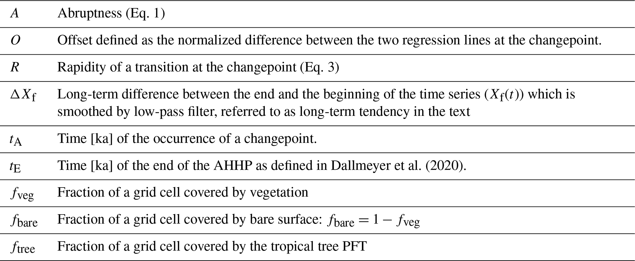
Trauth et al. (2018) suggested to identify abrupt events in paleo records by using the changepoint detection. The changepoint detection is a method of statistical time series analysis. It finds the time points at which the probability distribution of the time series changes. For our analysis, we choose the linear regression as statistical variable, and we decide a priori to find only one changepoint in linear regression, not an arbitrary number of changepoints, to focus on the most significant, step-like transition which we assume to be associated with the end of the Green Sahara.
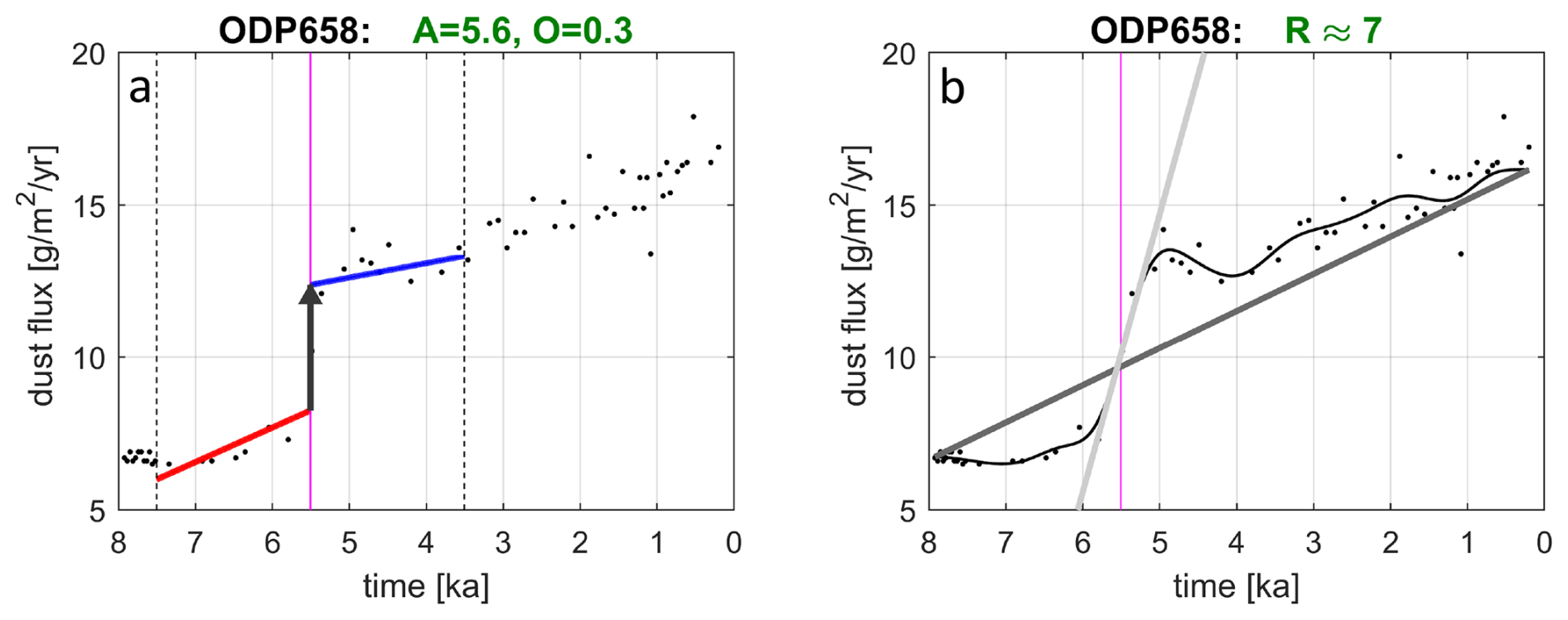
Figure 1(a) Abruptness in the dust flux record ODP658 (McGee et al., 2013). The black dots depict the data. The red line and blue line represent an optimum fit of two regression lines to the data in the interval (marked by vertical black dotted lines) before and after the changepoint (marked by the vertical magenta line). The offset O is defined as the difference between the two regression lines at the changepoint, here indicated by the length of the black arrow. The abruptness A is defined as the ratio of the offset O at the changepoint relative to the standard deviation in the data before and after the changepoint (Eq. 1). The title line indicates the offset O relative to the maximum change in smoothed dust fluxes in all marine cores (Fig. A3). (b) The black thin line shows the smoothed time series Xf(t) using a Butterworth filter of the order 5 and a cut-off frequency of years. The light gray straight line shows the slope at the changepoint which occurs at the time tA marked by the vertical magenta line, and the thick, dark gray line which depicts the long-term linear trend . The title line indicates the approximate rapidity R(tA) of the transition at the changepoint (Eq. 3).
Our analysis proceeds in the following steps: First, the entire time series is considered to find a changepoint in linear regression using the changepoint detection in MATLAB (The MathWorks Inc., 2018). Bathiany et al. (2020) recommend smoothing the time series and identifying the region of the strongest slope prior to the changepoint analysis. However, previous analysis of simulated vegetation time series (Dallmeyer et al., 2020) showed that the timing of the strongest slope strongly depends on the applied filter. In highly variable time series as analyzed in our study, this timing does not converge to a unique value in many cases. We therefore apply the changepoint analysis to the entire unsmoothed time series. We only interpolate the data to annual values to account for variable temporal resolution in the dust and pollen records and to ensure consistency between proxy data and simulations. Second, we follow the proposal by Bathiany et al. (2020), and we compute abruptness A as ratio between the offset O and the weighted sum of the un-detrended standard deviations of the data from the regression lines fitted to the data within a time interval before (i=1) and after (i=2) the changepoint. Hence:
where the weights are the ratios of the time spans before and after the changepoint (see Fig. 1 for visualization). Please note that A is a non-dimensional quantity.
We have investigated whether interpolating proxy data to annual values would affect the detection of changepoints by applying the changepoint detection to the time series with and without interpolation. It appears that the interpolation does not affect the detection of changepoints, except for some marginal cases like the marine record GC49 with an extremely coarse resolution (see Fig. 3). However, the values of abruptness generally differ between the analysis of interpolated and non-interpolated time series. We can attribute this reduction in abruptness to an increase in standard deviations from the linear regressions in the non-interpolated time series. Hence, we find it sensible to interpolate all proxy time series to the same resolution as the simulated time series, thereby putting the statistics of abruptness of data and model on the same basis.
For all dust and pollen records and simulated time series we ad hoc choose time spans of equal length of 2000 years before and after the changepoint (indicated by the vertical dashed line in Fig. 1a), such that as suggested by Bathiany et al. (2020). Only if the interval around the changepoint touches the beginning or the end of the data series, which only happens in a very few cases, we have to take different weights w1≠w2. This procedure limits the dependence of the value of A on the occurrence of the changepoint in the time series.
2.5.2 Definition of rapidity
In addition to the A and O values, we provide estimates of the approximate speed, or rapidity, R relative to a change in the external forcing of the climate system. Because the records considerably differ regarding the time resolution and because they reveal a strong variability, we have to interpolate the data to annual values and we smooth the interpolated time series X(t) by using a Butterworth filter (The MathWorks Inc., 2018) of the order 5 with a cut-off frequency . We use , because the temporal resolution ΔtR of the pollen records ranges from some 50 years to almost 400 years with a mean around 250 years and a median around 110 years (Table A1). This cut-off ensures smoothing of the original time series over at least two data points. For consistency, we apply the same filter strength to the dust-flux data, which show a much larger spread in the resolution with ΔtR≅130, 550, 990 years. For consistency, we also apply the same low-pass filter to the simulated time series, although the available time resolution of the simulations is one year. Next, we calculate the annual change of the smoothed time series Xf(t) at the time tA at which the changepoint occurs. The annual change is normalized by the difference ΔXf of 100-year averages of Xf(t) between the beginning and the end of the time series, divided by the time span ΔT of the record considered. In the following, we will simply refer to ΔXf as the long-term tendency. We define the relative change R(tA) at the time tA of the changepoint as the ratio of normalized change in Xf(tA) to the normalized change in external forcing F(tA) at the changepoint:
where ΔF is the amplitude of the forcing over the time span ΔT. During the mid- and late Holocene, the dominant long-term pre-industrial external forcing F(t) is the change in insolation caused by the variations in the Earth's orbit, i.e., mainly by the change in the climatic precession with a double period of some 19 000 to 23 000 years (e.g., Duque-Villegas et al., 2022; Rossignol-Strick, 1985). Here, we consider a transient simulation which covers the time period between 6000 BCE and 1850 CE and hence, we also use this time period for analysis of dust and pollen records. To a first approximation, the insolation in the tropics, more precisely: the meridional gradient in insolation, changes almost linearly during the last eight millennia. Hence, . Thus, Eq. (2) reduces to:
Because of the normalization, R(tA) is a non-dimensional quantity. There is some ambiguity in the interpretation of A and R values. These values themselves do not indicate whether an abrupt transition is a large or a small one; they just measure the abruptness relative to the internal variability of the time series or rapidity relative to the long-term trend. Therefore, values of A and R have always to be interpreted in view of their absolute values of the offset O and the long-term tendency ΔXf of the times series. Please note that in the simulations and in the pollen records, the long-term tendency ΔXf varies between 0 and 1. For the dust fluxes, we choose the maximum long-term tendency of 15.7 g m−2 yr−1 in the three dust flux records for a normalization. To exclude detection of spurious transitions, we exclude time series from the changepoint analysis with a small tendency ΔXf<0.1 and a small offset O<0.05. Such small differences over the entire mid and late Holocene or such a small jump at the abrupt change had presumably a negligibly small impact on climate and on Holocene fauna and people living in this region.
Please note that the precise values of A and R depend on parameters implicit in the computation of these values, like the thresholds ΔXf<0.1, O<0.05 and the width of the time interval around the changepoint at which the values A and R are computed. Varying these thresholds and parameters (which we did not show here) does change the numbers of A and R, but the general spatial patterns and characteristics of transitions in data and simulation and, hence, the qualitative conclusions remain the same.
3.1 Patterns of long-term tendencies, abruptness and rapidity
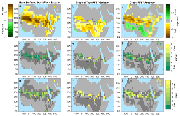
The pattern of simulated long-term tendencies ΔXf of bare surface fraction between mid-Holocene and pre-industrial shows large values in a north-west to south-east oriented strip between 20° N in the west and 15° N in the east, which extends between two and four grid boxes in the north-south direction, corresponding some 400 to 800 km (its center is indicated by a thin black line Fig. 2). To the north and to the south of this strip, long-term tendencies are considerably smaller. In the grid boxes indicated by a light gray color, the long-term tendencies between the beginning and the end of the simulations are smaller than ΔXf<0.1. This simulated pattern of long-term tendencies matches the reconstructed long-term tendencies in the Saharan taxa and in the dust deposition found in the marine sediment cores at around 20° N and north of it at 23° N, as far as we can judge from the few available records (Fig. 2a). The north-west to south-east oriented pattern of changes in bare surface, and hence total vegetation cover, reflects the known tilted moisture gradient across North Africa as documented in present-day's vegetation maps (Dinerstein et al., 2017; Sayre et al., 2013; White, 1983) and palynological records (Dinies et al., 2026). The MPI-ESM apparently captures this tilted gradient in vegetation across the region (Fig. A4).
The pattern of long-term tendencies in the simulated tropical tree PFT, i.e., the sum of the fractions of evergreen and deciduous tropical tree PFTs, is consistent with the tendency in the Guinean group found in the pollen records (Fig. 2b). The long-term tendencies in simulated grass PFT and in Poaceae also by and large match (Fig. 2c). In the Lake Yoa record (Kröpelin et al., 2008; Sylvestre et al., 2026), the proportions of Poaceae decline, so does the fraction of simulated grass PFT in this region during mid- and late Holocene. In almost all pollen records near the Atlantic coast at roughly 15–16° N (with the exception of the Touba N'Daye record, see Sect. 3.2) and in the Manga grasslands at around 13° N and 11° E, the proportion of Poaceae increase. In the model, the increase in the fraction of grass PFT is found south of 15° N in the west and some 10° N in the east, i.e., the border between decrease and increase in grass PFT in the model is located a bit, perhaps one grid box, to the south in comparison with pollen data.
The geographic patterns of abruptness in simulations and proxy data are shown in Fig. 2d–f. Abrupt transitions with an offset O≥0.05 at the changepoint in linear regression, indicated by green to yellow shades, appear within the region of the largest decrease in bare surface fraction and largest increase in Poaceae over the last 8000 years (Fig. 2a, c). In the grid boxes indicated by a dark gray color to the north and the south of the abrupt transitions, either no changepoints, and hence no abrupt step changes, or abrupt step changes, but with a small offset O<0.05 are found as shown in more detail in Sect. 3.2. In some dark gray grid boxes, abrupt transitions with a negative abruptness value are found.
Figure 2d–f show that the abrupt transitions in bare surface fraction fbare generally appear to be less abrupt, measured in terms of A values with A≤3 and indicated by green and dark green colors, than the transitions in the tropical tree and grass PFTs, indicated by lighter green and yellow colors with abruptness values up to A≈6. On average, the abruptness of transitions in the tropical tree PFT and grass PFT are a factor of 2 and 1.3 times, respectively, larger than the abruptness of transitions in bare surface fraction. This result implies that the transition in the type of the vegetation cover, i.e. in tropical tree and grass PFTs, is more abrupt than, and in a very few grid boxes even more than twice as abrupt as, the transition in the total vegetation cover. There are a very few exceptions, almost all of it are located at the Levant and at the northern rim of the Ethiopian Highlands, i.e., in grid boxes outside of our region of interest.
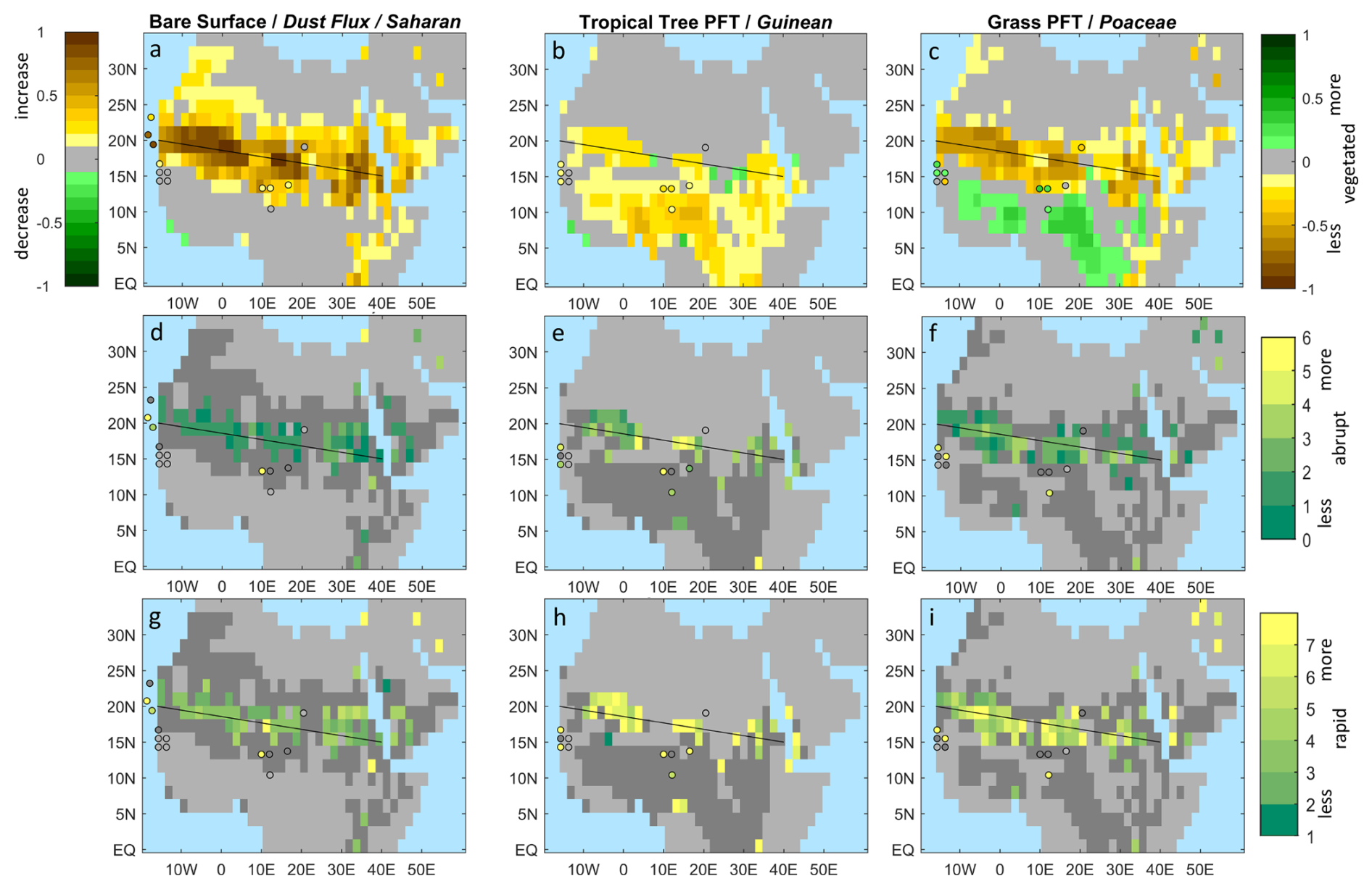
Figure 2Long-term tendencies ΔXf (a-c), abruptness A (Eq. 1) (d-f) and rapidity R (Eq. 3) (g-i) of simulated fractions of bare surface and Saharan taxa and dust flux (a, d, g), simulated tropical tree PFT and Guinean taxa (b, e, h) and simulated grass PFT and proportions of Poaceae (c, e, i). The shades show simulations and the colored dots, data. Gray colors indicate time series with small long-term tendencies ΔXf<0.1 in simulated bare surface, PFTs and data. Dark gray shades in (d–i) indicate grid boxes and records for which no changepoint is found or a change point with a small offset O<0.05 or a negative offset. Please note that the changepoints at which the abruptness and rapidity are evaluated occur at different times for different grid boxes and proxy records. The patterns of occurrence of changepoints is shown in Fig. 7c, d. The scale of color bars is chosen to best visualize the patterns of change. Figure 2d–f and g–i, respectively, share the same color bar. The color bar for Fig. 2a is inverted in comparison with the color bar for Fig. 2b, c.
The geographic patterns of the rapidity R (Eq. 3) at the changepoint are presented in Fig. 2g–i. If a transition in the simulation or in the proxy records would directly follow the approximately linear change in the insolation forcing, then the rapidity is approximately one, i.e., R≅1, shown as dark green color in Fig. 2g–i. On average, the simulated bare surface fraction increases some four times faster than the approximately linear trend in orbital forcing, i.e., R≈4. Only in a very few isolated grid boxes and in the Saharan taxa of the Lake Bal record, more rapid transitions occur. Transitions in tropical tree and grass PFTs obviously occur not only more abruptly, but also more rapidly, with values of R>7, than the transition in bare surface fraction. The high R values for tropical tree PFT and grass PFT are consistent with the high R values found for Guinean taxa and Poaceae in the few pollen records for which abrupt transitions are found (Lake Guiers, Lake Diogo, Lake Bal, Lake Tjéri, Lake Tilla).
3.2 Focus on regions and individual records
In the western Sahara at around 20° N, the degree of abruptness in simulated bare surface is much smaller than the degree of abruptness in the dust fluxes reconstructed from the marine Atlantic cores ODP658 and GC68 (Fig. 3). Figure 3 also shows that the transition in simulated bare surface at around 20° N and south of it is more characterized by a strong increase in the average slope of the time series rather than by a step-like transition. In these cases, the offset at the changepoint is small or even negative. A negative offset implies an abrupt change in the opposite direction of the long-term tendency. Two extreme cases with a negative offset are depicted in Fig. 3 (in the second row of grid boxes). We show that the latter cases can be attributed to a model artefact (see Appendix B).
At approximately 25° N (upper line of grid boxes in Fig. 3), the rather gradual increase in simulated bare surface matches the gradual transition in the dust flux in the GC49 record. In fact, the long-term tendencies in simulated bare surface and reconstructed dust are small (indicated by bright yellow color in Fig. 2a) and if a changepoint is detected, then the offset at the changepoint is very small (O<0.05) or negative (dark gray colors in Fig. 2d).
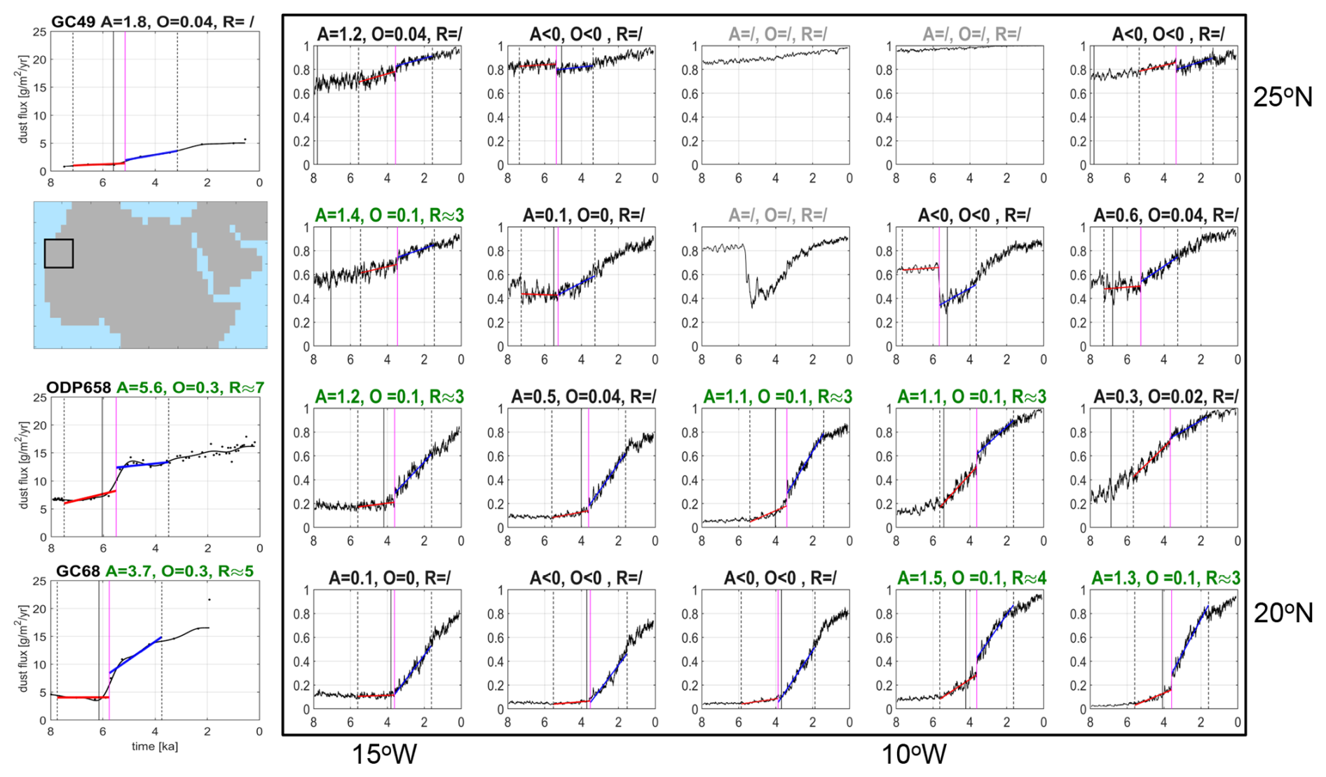
Figure 3Time series of dust flux reconstructed from records GC49, GC68 and ODP658 (left boxes) and simulated bare surface fraction in the western Sahara near the Atlantic coast (see small map at the top left). The x-axes indicate the time ranging from 8 to 0 ka, and the y-axes, the dust flux in g m−2 yr−1 for the marine records and the bare surface fraction for the simulations, where 0 refers to a fully covered by vegetation and 1, a completely barren, non-vegetated surface. The title lines indicate the values of abruptness A (Eq. 1), absolute offset O, and rapidity R (Eq. 3) at the changepoint in linear regression of the time series. The dots in the data boxes indicate the data points, the thin black curve shows the filtered time series Xf(t). The red and blue straight lines represent the linear regression before and after the changepoint. The vertical magenta line depicts the time tA at which the changepoint occurs, and the vertical black dashed lines indicate the time interval around tA used to calculate A. The vertical full black line indicates the beginning of the end of AHHP, labelled tE (explanation see Sect. 3.3). Green titles indicate step-like transition with a long-term tendency ΔXf≥0.1, abruptness values A>1 and an offset O≥0.05, light gray titles, a transition with a small long-term tendency ΔXf<0.1, and black titles, an abrupt jump with a negative offset or a small offset O<0.05 or a time series for which no changepoint is found. In the latter case, one linear regression line is shown.
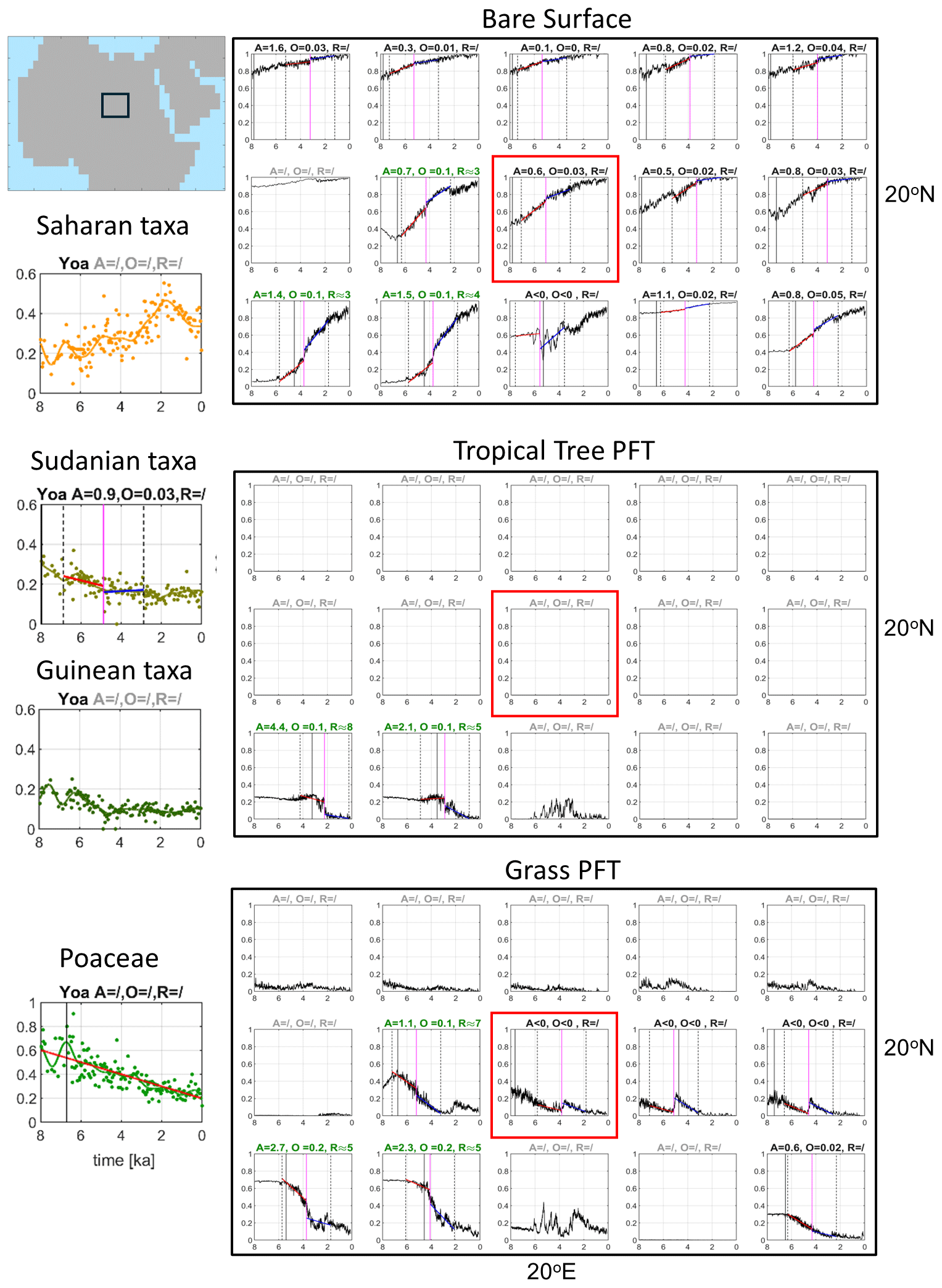
Figure 4Same as Fig. 3, except for time series of Saharan, Sudanian, Guinean taxa and Poaceae from the Lake Yoa record (left boxes) and simulated fractions of bare surface, tropical tree PFT and grasss PFT in the region around the Lake Yoa (large black boxes). Please note that the scale of the y-axes differs: for Saharan, Sudanian, Guinean taxa, the y-axes range from 0 to 0.6, for Poaceae and all simulated time series, from 0 to 1. The location of these grid boxes is shown in the small map at the top left of the figure. The red box inside the large boxes depicts the grid box in which the Lake Yoa is located.
For the Lake Yoa record (Fig. 4), the times series of bare surface and grass PFT in the grid box in which the record is located (marked by a red box) do not resemble the time series of phytogeographical groups found in the record. The Lake Yoa record shows a dominance of Sudanian taxa and high, but fluctuating proportions of Guinean and Saharan taxa during the first millennia (8 to 6 ka), and a dominance of Saharan taxa with small, but clearly visible proportions of Sudanian and Guinean taxa in the late Holocene after around 4 ka. No tropical tree PFT is found in the grid box that includes the Lake Yoa location. The simulated time series to the south-west of the Lake Yoa grid box much better match the pollen record. This is consistent with the dry bias of the MPI-ESM: the model predicts a somewhat smaller northward extent of the mid-Holocene Green Sahara than found in reconstructions (Dallmeyer et al., 2020). A comparison of the Lake Yoa pollen records with the simulated PFTs in the grid boxes to the south-west of the Lake Yoa grid box thus appears to be more sensible.
The simulated bare surface fraction in the grid boxes southwest of the Lake Yoa grid box starts to increase slightly already at 8 ka with an accelerated increase after around 6 ka and a step-like increase with however a small offset and abruptness (). The Saharan taxa fluctuate during 8 and 6 ka, followed by two periods of distinct increase about 6 and 3 ka. The marked decline after 2 ka is presumably caused by increasing land use at the Lake Yoa (Lézine et al., 2011) evident by an increase in doum and date palm (Hyphaene and Phoenix) (Dinies et al., 2026), yet climate variations cannot be excluded (Sylvestre et al., 2026). Without the marked decline at 2 ka, the dynamics of the simulated bare surface and the Saharan taxa would likely be similar.
The tropical tree PFT in the grid boxes southwest of the Lake Yoa grid box decline abruptly with a small offset (O≈0.1) at around 4 ka, roughly some 2000 years later than the Guinean and Sudanian pollen groups which start to decline already around 6 ka. Similarly, the simulated grass PFTs decline more rapidly and later than the Poaceae do. This result is consistent with the tendency of a later end of humid conditions of the AHHP found in the MPI-ESM (Dallmeyer et al., 2020). Pollen records from the Sahelian west coast of Africa (Fig. 5) are characterized by lower proportions of Saharan taxa compared to the Lake Yoa record. An abrupt increase in the Saharan taxa only occurs in the northernmost Lake Guiers pollen record, but with only a very small offset O<0.05 (therefore shown as dark gray dot in Fig. 2a). This transition appears more as a distinct change in the slope of the regression lines fitted to the data rather than as an abrupt jump in the data as seen in most time series of bare surface fraction in the uppermost row of grid boxes in Fig. 5 and in the western Sahara (Fig. 3).
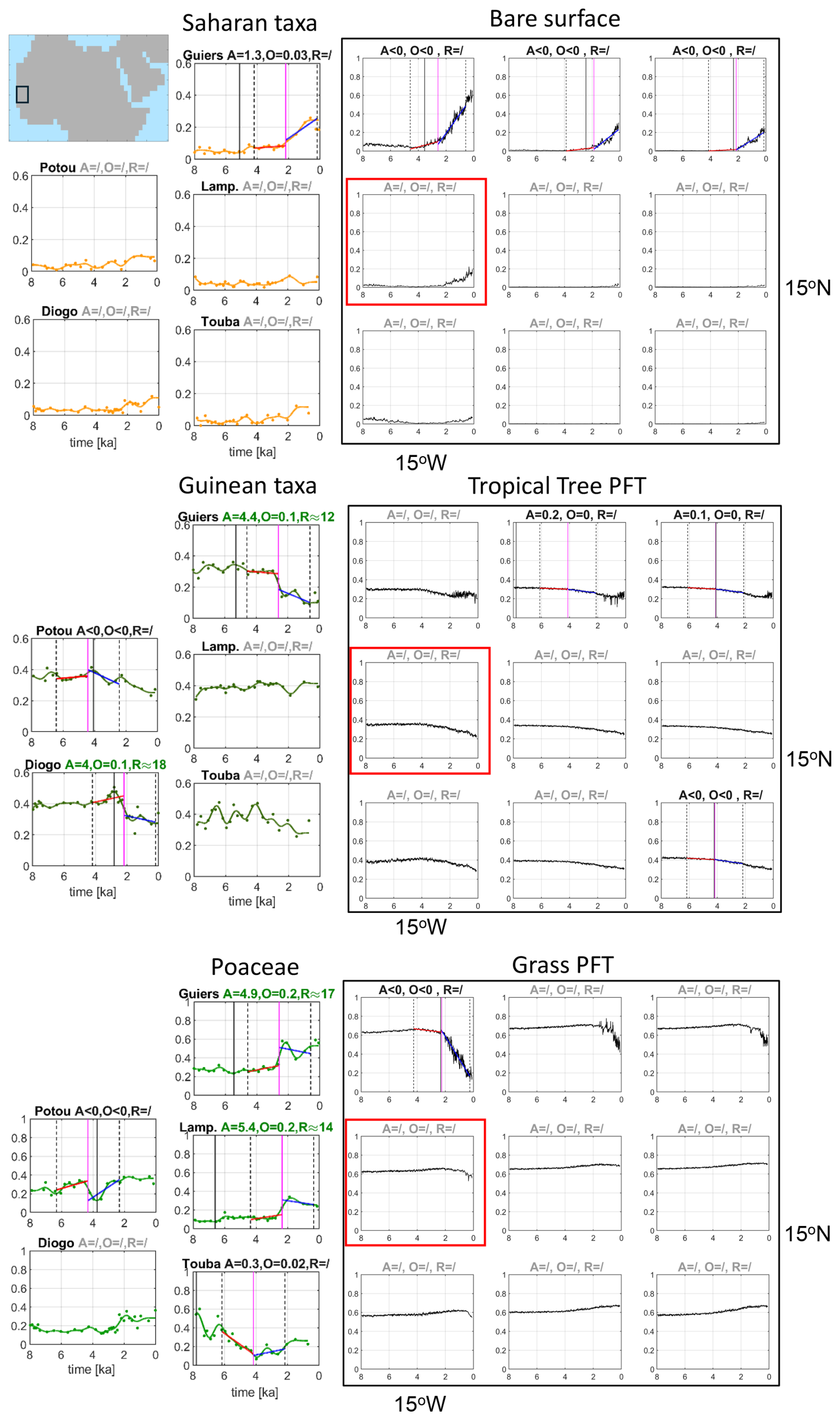
Figure 5Same as Fig. 3, except for time series of Saharan and Guinean taxa and Poaceae from the pollen records in the western Sahelian region (left boxes) and simulated fractions of bare surface, tropical tree PFT and grass PFT in this region (large black boxes) as shown in the map at the top of the figure. All pollen records are located within grid box marked in red.
Guinean taxa (and Sudanian taxa, Figs. A2, C1) display clearly higher proportions at the west coast than at the Lake Yoa, so does the simulated tropical tree PFT. Guinean (and Sudanian) taxa generally decline, like the simulated tropical tree PFT. The long-term decline is, however, small (i.e., ΔXf<0.1) in most grid boxes and records. In the Guiers record, an abrupt decline in Guinean taxa (and in Sudanian taxa, along with an abrupt increase in Sahelian taxa, Fig. C1) is detected at approximately the same time of the abrupt increase in the slope of the time series of Saharan taxa around 2 ka. The other pollen records do not show abrupt changes in the phytogeographical groups, except for the Guinean taxa in the Diogo record. The abrupt decline in Guinean taxa in the latter record is, however, preceded by a rapid increase and could thus be interpreted as part of a large fluctuation.
The dynamics of Poaceae differ considerably among the west Sahelian records which are located in close proximity of some 200 km: step-like increase at the Guiers and Lampoul sites, an increase, but a negative jump (A<0) at the Potou site, no significant long-term tendency at the Diogo site, and an abrupt decline, but rather as a marked change in the slope at the Touba site. The simulated grass PFTs in this region show marginally increasing trends and only in the northernmost grid box, a sharp decline at around 2 ka in contrast to the data.
The trends in the proportions of Saharan taxa in the Lake Bal, Lake Jikariya and Lake Tjéri records, located in the central Sahelian region, and the Lake Tilla record, located in the central Sudanian region, and the simulated bare surface fraction in this region qualitatively agree (Fig. 6). In the central Sahelian records the Saharan taxa abruptly increase between 4 and 3 ka, although only at the Bal site an abrupt step-like increase is found, while in the other two records, the increase emerges as a strong change in the slope of the time series. The simulated bare surface fractions reveal a similarly distinct change in the slope of the time series a bit later, shortly after 3 ka and around 4 ka in the grid boxes in the northern part of this region. The very small fractions of simulated bare surface with their only slightly increasing trends in the southernmost grid boxes are consistent with the small proportions and a slight increase in Saharan taxa at the Lake Tilla site located in the Sudanian region.
Both, the simulated tropical tree PFT and the Guinean taxa decline throughout the last 7000 to 6000 years in the central Sahelian and the Sudanian region, but their dynamics differ. The fractions of simulated tropical tree PFT decline gradually and rather smoothly. The Guinean taxa reveal abrupt declines, although the jump in Guinean taxa at the Tilla site is small (O≈0.1) and at the Jikariya site, it is negative (O<0). The abrupt change in the Guinean taxa in the Tjéri record seems to be caused by the large scatter in the data around 7 ka. The Sudanian taxa (Fig. C1) show a large variability with no clear trend.
Opposite trends are found in simulated grass PFT and in Poaceae, as already seen in Fig. 2c. The proportions of Poaceae in the four records basically increase during the last 8000 years with distinct fluctuations. The simulated grass PFTs increase only slightly, if at all, from 8 to 3 ka and clearly decrease thereafter. Only in the grid boxes, in the very south east of this region, simulated grass PFT tend to increase, qualitatively matching the trend in Poaceae in the Tilla record.
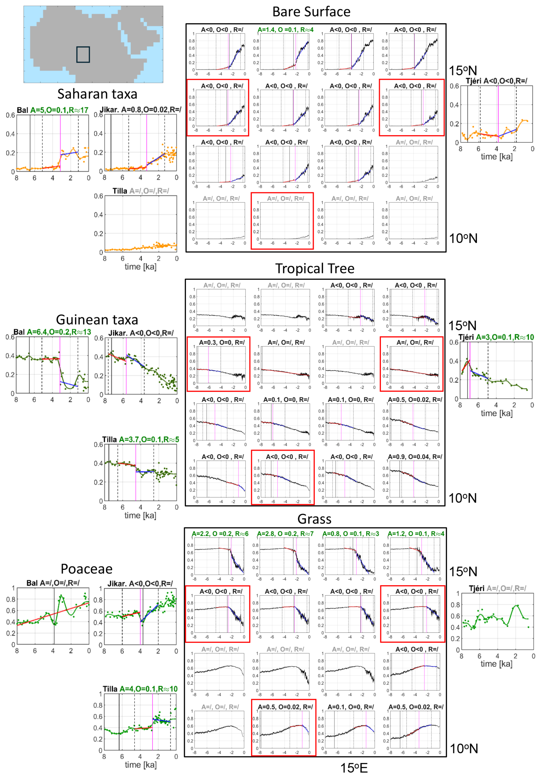
Figure 6Same as Fig. 3, except for time series of Saharan and Guinean taxa and Paoceae from the pollen records in the central Sahelian sites (Lake Bal, Lake Jikariya, Lake Tjéri) and central Sudanian region (Lake Tilla) and simulated fractions of bare surface, tropical tree PFT and grass PFT in this region (large black boxes) as shown in the map at the top left of the figure. The red boxes indicate the location of the pollen records in the model grid. Please note that the Lake Bal and Lake Jikariya sites are located in the same grid box.
To summarize the focus on regions and individual records, most pollen records show large fluctuations in the time series of taxa. In only half of the records, we find clear, step-like abrupt transitions in the taxa with large offset and abruptness values (). The dynamics of the transition in taxa vary even between records in close proximity, like in the western Sahel region at the Atlantic coast and in the Manga Grasslands (Lake Bal and Lake Jikariya) in the central Sahelian region. But it is also evident that dynamics in simulated bare surface fraction are consistent with the dynamics in Saharan taxa: abrupt changes emerge rather as an abrupt increase in the average slope of the time series with a small abruptness A than as an abrupt step-like transition, with the exception of the Lake Bal record (and the Lake Yoa record which, however, we have to ignore in this respect).
3.3 How does the timing of abrupt changes in PFTs and pollen taxa relate to the end of the AHHP?
Dallmeyer et al. (2020) calculated the end of the AHHP based on the smoothed simulated time series of changes in the bare surface fraction and compared the simulations with data by Shanahan et al. (2015). In short, Dallmeyer et al. (2020) formally define the time tE of the end of the AHHP in the following way: The slope between two consecutive time steps of the smoothed time series of simulated bare surface fraction has to exceed the slope of a straight line between the beginning and the end of this time series. In addition, the minimum of the bare surface fraction has to precede tE and after 500 years, the slope has still to be larger than the slope of the straight line (for visualization of the slope method, see Fig. 1 in Dallmeyer et al., 2020).
The pattern and values of tE(fbare) (Fig. 7a) agree with those found in Dallmeyer et al. (2020) which were calculated for a different realization of the same ensemble of MPI-ESM Holocene simulations. Specifically, the simulations show a very early start of aridification in the northern part of the Sahara and a clear transgressive termination tE starting earlier in the north than in the south and earlier in the east than in the west at the same latitude in qualitative agreement with the hydrologic data by Shanahan et al. (2015). In the region south of 20° N in the west and 15° N in the east, indicated by the thin black line in Fig. 7, the simulated bare surface fraction starts to increase only during the late Holocene after around 4 ka. The majority of records, however, indicate an distinctly earlier end in terms of tE for dust fluxes and Saharan taxa, which is also consistent with the tendency of a later end of the simulated AHHP in the MPI-ESM found by Dallmeyer et al. (2020), mentioned above.
The time tE(fbare) precedes the time tA(fbare) of the abrupt change in the simulations and in all dust and Saharan taxa at all sites for which an abrupt change is detected (Fig. 7a, c, e). This result is to be expected, because tE(fbare) indicates more the beginning of the end of humid conditions, i.e. the beginning of an increasing trend of bare surface fraction and Saharan taxa, while at the time tA(fbare) of the abrupt change, the transition towards more arid conditions and, hence, a more barren landscape is in full swing.
Lemonnier and Lézine (2022) suggested that the first decrease of proportions of the wettest plant formation indicates the end of the AHHP. Our simulations are consistent with this suggestion, i.e., tE(ftree)≤tE(fbare), when considering the region south of 15° N, i.e., the region where tropical trees predominantly occurred (Fig. 7a, b). In contrast to the general progression from the north to the south found in the timing tE of simulated bare surface fraction, the fractions of simulated tropical PFTs generally start to decline earlier east of around 10° E than in the west, almost independent of the latitude. Hence the first sign of a decline in simulated tropical PFTs shows a continentality gradient in contrast to the north-south oriented of simulated bare surface fraction. Like for the simulated bare surface fraction, the timing of an abrupt change in simulated tropical tree PFT (and grass PFT, not shown here) and for all other taxa, Sahelian, Sudanian and Guinean (Fig. C1) occur after the earliest indication of a trend towards aridification, i.e., tA(ftree)>tE(ftree) (Fig. 7f). Exceptions are cases of abrupt transitions with A<0, e.g. for Poaceae at the Potou and Jikariya sites (Fig. C1).
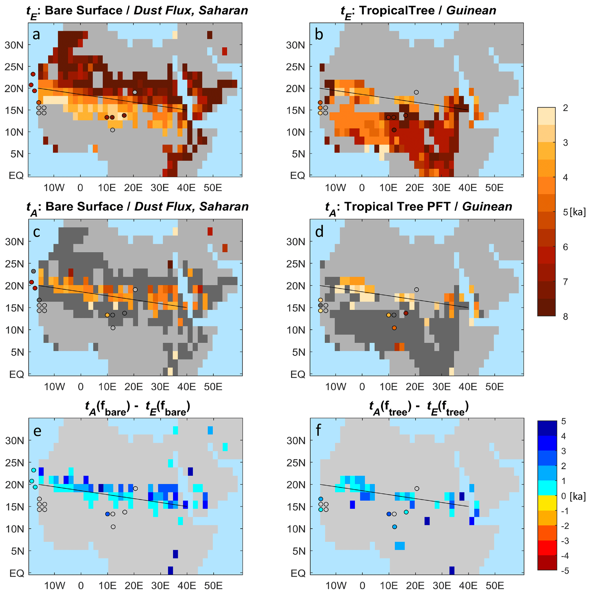
Figure 7(a, b) depict the patterns of tE [ka], defined as timing of the beginning of the end of the Green Sahara as computed by the slope method of Dallmeyer et al. (2020) and (c, d) show the time tA [ka] at which a changepoint in linear regression of time series is found. Gray shades refer to small long-term tendencies with ΔXf<0.1, dark gray shades, to grid boxes for which no changepoint is found or a changepoint with a small absolute offset or a negative offset. (e, f) indicate the differences tA−tE [ka]. Blue colors imply that tE precedes tA.
3.4 Unstable or stable collapse?
Are the abrupt changes in bare surface and PFTs found in our simulation related to abrupt changes in precipitation which, to a first approximation, is the main climatic driver of Saharan vegetation? Liu et al. (2006) proposed distinguishing between an “unstable collapse” and a “stable collapse” of Saharan vegetation cover at the end of the AHHP. An unstable collapse of Saharan vegetation cover is supposed to be caused by a strong positive feedback between precipitation and vegetation which can be detected by a synchronous abrupt change in vegetation cover and precipitation like in the models of Brovkin et al. (1998) and Claussen et al. (1999). A stable collapse emerges from a weakly positive feedback between precipitation and vegetation which leads to an abrupt vegetation decline once a threshold in precipitation is crossed without causing an abrupt change in the precipitation. In his conceptual mathematical model Liu et al. (2006) used a 10-year average of precipitation instead of annual mean precipitation for the following reason: Saharan vegetation does not directly depend on precipitation, but mainly on surface soil moisture and subsurface moisture with a persistence time of decades. This is because perennial grasses and trees especially in seasonally dry tropical environments, also have a proportion of deep roots that can be crucial for their survival through the dry season. As such, subsurface soil moisture provides a long-term memory effect for grasses and trees. These long-term effects of climate variability and soil moisture are approximated as a 10-year running mean of a stochastic annual mean precipitation forcing in the model of Liu et al. (2006).
Do we find any abrupt changes in the 10-year mean precipitation in our MPI-ESM Holocene simulation? The answer to this question is simply: no, we have not found any significant changepoints in the 10-year mean precipitation (nor in annual mean precipitation, not shown here). In most, if not all, grid boxes, the simulated 10-year mean precipitation decreases almost linearly. If changepoints emerge, then the offset at the changepoint and, thus, the abruptness is very small or negative. The grid boxes in the south-west corner of the Lake Yoa region provide an illustrative example (Fig. 8).
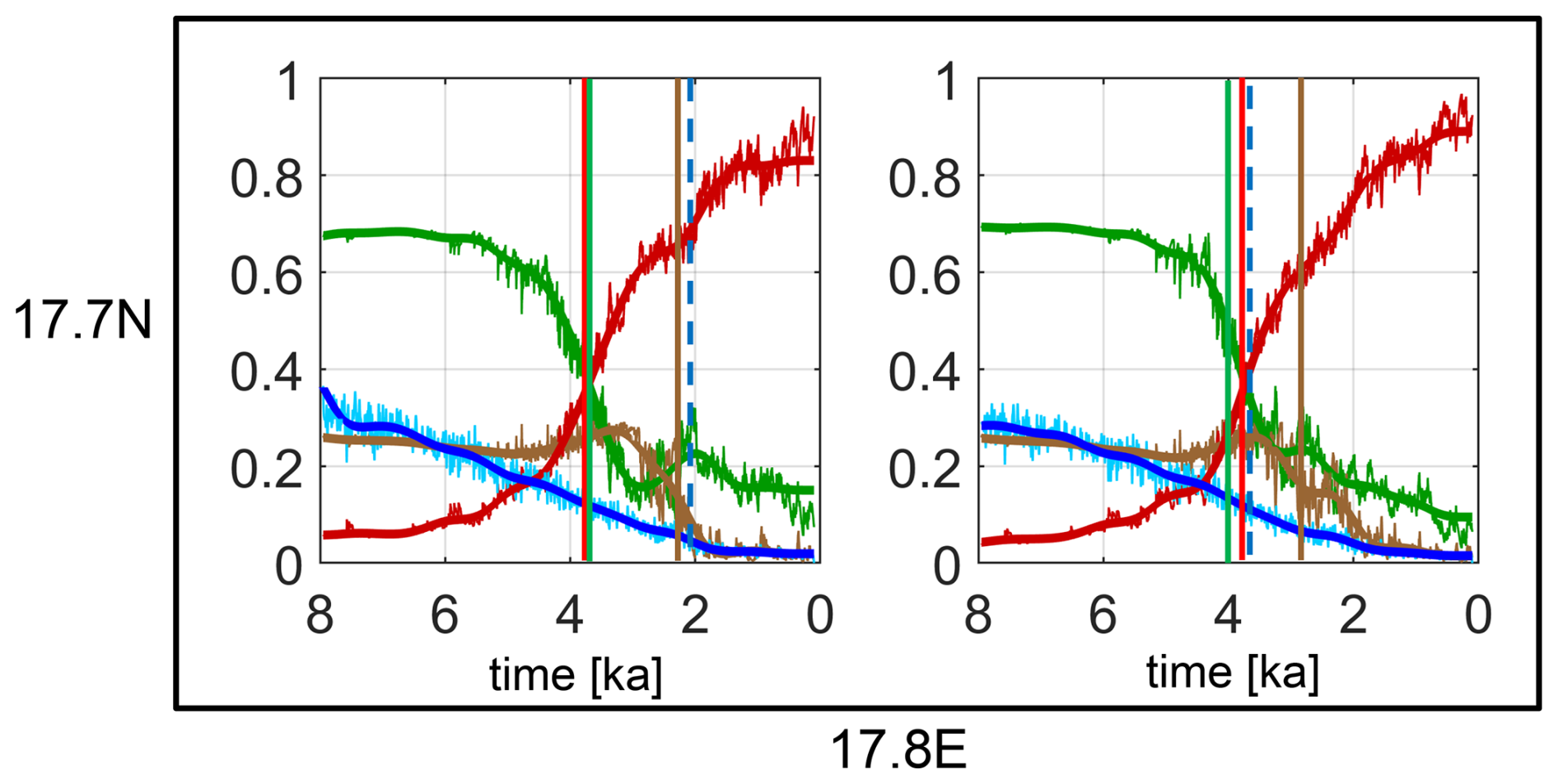
Figure 8Time series of simulated bare surface fraction (red lines), grass PFT (green lines), tropical tree PFT (brown lines), and 10-year mean precipitation (blue lines) for two grid boxes in the south-west corner of the Lake Yoa region (see Fig. 4). The thin lines depict annual mean bare surface fraction, grass PFT, tropical tree PFT and 10-year mean precipitation, respectively, and the thick lines are the smoothed time series. The colored vertical straight lines show the respective changepoints. The dashed blue vertical line indicates that offset at the changepoint in the 10-year mean precipitation is negligibly small.
In the theory of stable vegetation collapse, it is supposed that abrupt vegetation changes occur, once a threshold in precipitation is crossed. To answer the question of whether the abrupt transitions in bare surface and PFTs found in our simulation are related to a threshold in the 10-year mean precipitation, we analyse all abrupt changes in the region of largest long-term changes and abruptness values, i.e., for all grid boxes between 23.3 to 14.0° N and 15.0° W and 35.6° E. Indeed, the histograms for tropical tree PFT and grass PFT show a clear maximum at the intervals between 100 to 150 and 250 to 350 mm yr−1, respectively. In contrast, the histogram for bare surface fraction is rather flat (Fig. 9). The threshold in 10-year mean precipitation at the changepoint for tropical tree PFT is considerably smaller than that for grass PFT. In most grid boxes in question, the transition from a Green Sahara to a desert obviously proceeds from a lush green grass savanna to a sparely vegetated tree savanna and, finally, to a desert – see Fig. 8 as illustrative example. And because of this step-wise change in the ecosystems, the changes in bare surface cannot be associated with a unique threshold in precipitation.
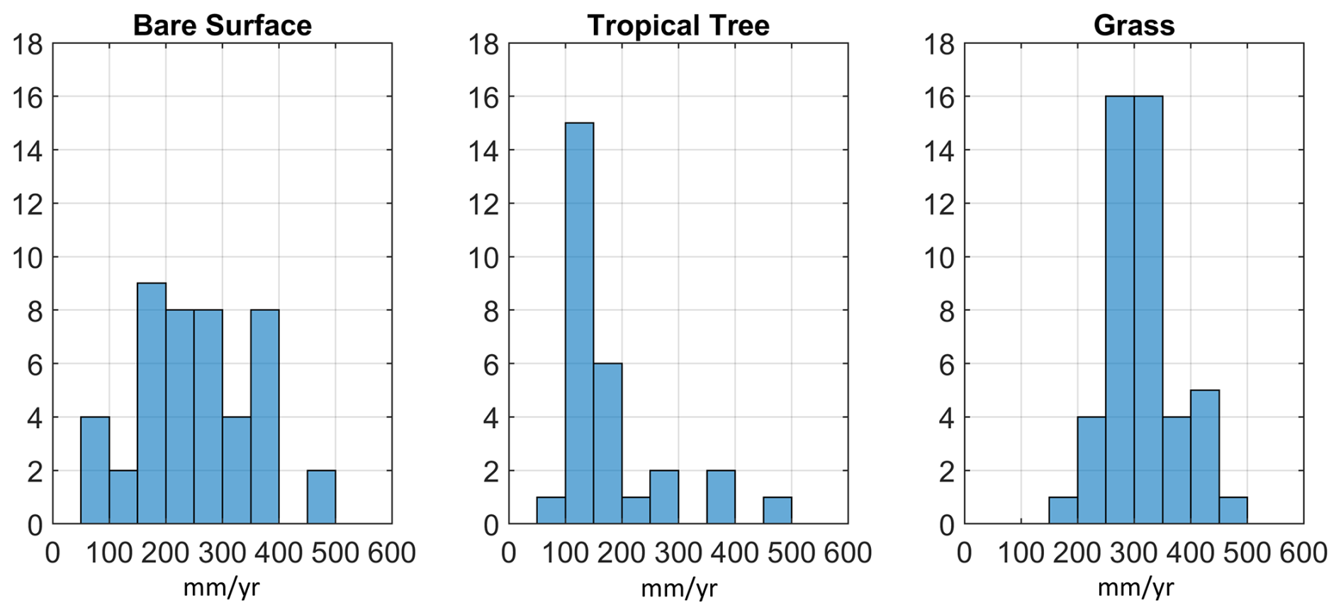
Figure 9Histograms of values of annual mean precipitation at the changepoints in bare surface fraction, tropical tree PFT and grass PFT, respectively. The histograms are computed for all changepoints in the region of the largest vegetation changes, i.e., for all grid boxes between 23.3 to 14.0° N and 15.0° W and 35.6° E.
Perhaps just by fortuitous coincidence, the abrupt vegetation collapse in the model of Liu et al. (2006) is associated with a threshold in 10-year mean precipitation of some 300 mm yr−1 which by and large agrees with the threshold for grass PFT found in our simulation. It should be noted, however, that the conceptual model of Liu et al. (2006) does not distinguish between grass and tree cover, but represents total vegetation cover using parameters characteristic of the predominantly grass-covered southern Sahara. In our complex dynamic vegetation model, we find the threshold behavior in the vegetation composition, rather than in the total vegetation cover. The spread of the histograms shown in Fig. 9 suggests that other climatic drivers than precipitation also affect the abrupt changes found in our simulation.
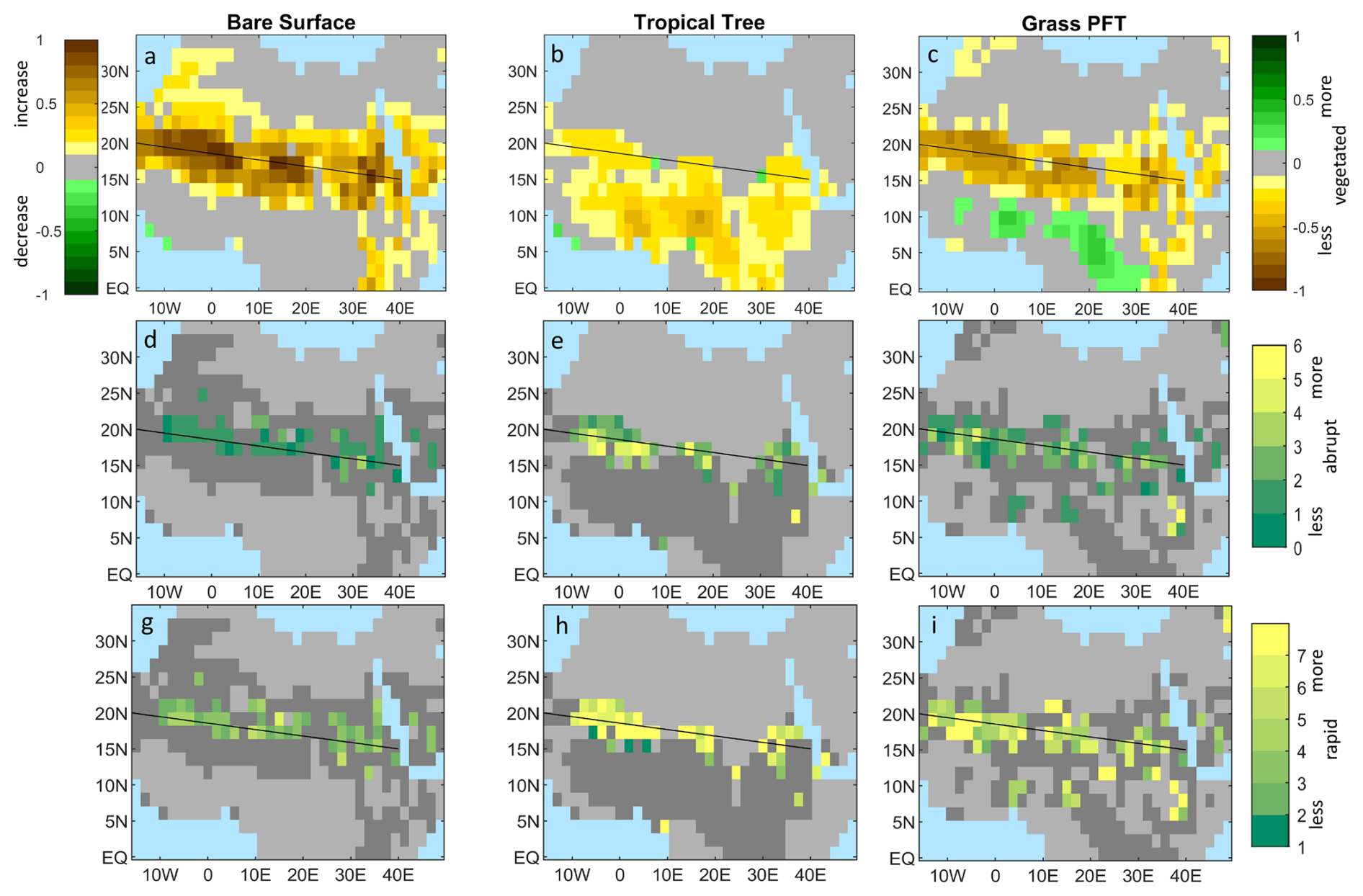
Figure 10Same as Fig. 2 but for a slightly different MPI-ESM Holocene simulation driven by the same orbital forcing, but a stronger volcanic forcing causing a larger internal climate variability (Please note that the region shown in this figure slightly differs from the region shown in Fig. 2.).
4.1 Defining and quantifying abruptness
To move beyond the long-standing qualitative debate on an abrupt versus gradual termination of the Green Sahara at the end of the AHHP, abruptness must be explicitly defined and translated into a standardized and comparable measure. For this purpose, we have developed a changepoint-based metric that quantifies the rate of change during the identified transition relative to the long-term background trend. Although this metric provides a novel, standardized approach, the resulting estimates of abruptness and rapidity depend on several methodological parameters and should therefore not be interpreted as absolute characteristics of the respective time series. Instead, the method provides an internally consistent framework for quantitatively comparing the relative abruptness and rapidity of transitions across simulations and proxy records.
Our metric is based on detecting a single changepoint in linear regression of each time series because our analysis focuses on dominant step-like transitions. Most of the simulated time series and proxy records considered here contain one pronounced transition, expressed either as a step change or as a marked change in trend. In these cases, a single-changepoint framework provides a transparent and readily comparable characterization of the transition. Some grid boxes and proxy records, however, exhibit only weak long-term trends superimposed by large fluctuations or multiple smaller transitions. Our metric was not designed to characterize such variability. These time series could instead be analysed using multiple-changepoint approaches, as applied, for example, to the long Chew Bahir record by Trauth et al. (2018). Extending the framework in this direction would, however, raise new questions about the quantitative meaning of abruptness. It is not obvious whether abruptness should then be represented by the number of changepoints, the magnitude or rapidity of the strongest transition, or an aggregate measure incorporating all detected changes. Developing a metric that consistently captures such complex, multi-stage dynamics therefore remains an important topic for future research.
4.2 Robustness of results
Are the patterns of largest vegetation changes and abruptness presented in Sect. 3.1 and 3.2 robust or are they mainly determined by random climate fluctuations? If internal climate variability dominates, then other Holocene simulations with the same ESM would yield grossly different results. We have not available a large ensemble of transient Holocene simulations with the same MPI-ESM. We can however use a similar Holocene simulation with the same MPI-ESM-1.2 which is driven by the same orbital forcing, but stronger volcanic forcing (Bader et al., 2020; Dallmeyer et al., 2020). The stronger volcanic forcing causes a somewhat stronger internal climate variability than the weaker, and more realistic, volcanic forcing used in the simulation analyzed here. It appears that the geographic patterns of largest vegetation changes, abruptness and rapidity of abrupt changes in the simulation with a stronger volcanic forcing remain very similar to those found in the simulation with the weaker volcanic forcing (compare Figs. 10 and 2).
Indeed, a focus on the western Sahara (Fig. 11) reveals that the two simulations differ only on short time scales, but not on much longer time scales, nor in the long-term trend. Only the “cumbersome” grid boxes discussed as model artefacts in the Appendix B show a somewhat larger deviation between simulations. Such grid boxes are rare exceptions from the rule when considering all grid boxes of our study area. We therefore conclude that our results are robust i.e., they are primarily determined by the deterministic orbital forcing and are influenced only to a small extent by internal climate variability.
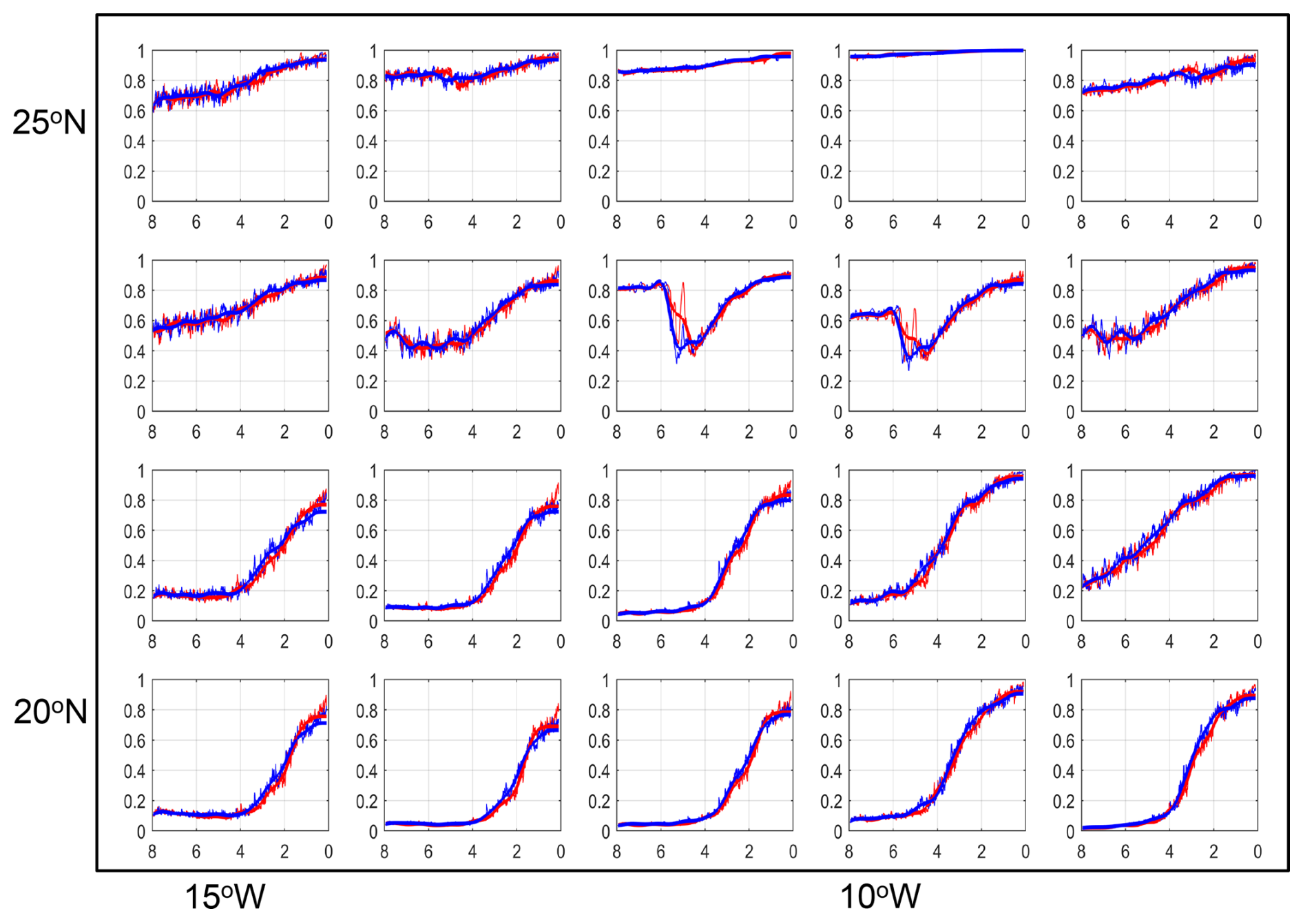
Figure 11Focus on simulated bare surface fraction in the western Sahara region (compare with Fig. 3). The blue lines depict the results of the simulation used in this study. The red lines depict results from a slightly different MPI-ESM Holocene simulation driven by with the same orbital forcing, but a somewhat stronger volcanic forcing causing a slightly larger internal climate variability on short time scale.
4.3 Climatic drivers of simulated vegetation transitions
In Sect. 3.4, we compared abrupt changes in the simulated plant functional types (PFTs) with changes in precipitation to assess whether the transitions identified in our analysis are consistent with strong climate–vegetation feedbacks. We used 10-year mean precipitation as a common indicator of climatic forcing to facilitate comparison with the conceptual framework of Liu et al. (2006). This approach necessarily simplifies the climatic drivers of vegetation change. Neither in JSBACH nor in natural ecosystems is vegetation determined by precipitation alone.
The principal external forcing of the simulated Holocene climate evolution is the orbitally driven change in the seasonal distribution of insolation. Enhanced Northern Hemisphere summer insolation during the early and middle Holocene strengthened the African monsoon, increased moisture availability and supported the expansion of vegetation across the Sahara during the AHHP. As summer insolation subsequently declined, the monsoon weakened and its northern margin retreated. However, orbital forcing also altered the seasonal cycles of temperature, precipitation and radiation, as well as sea-surface temperatures and the land–sea thermal contrast.
Dallmeyer et al. (2021) showed that even within the Sahel–Sahara region, simulated Holocene changes in vegetation composition in MPI-ESM-1.2 were controlled by both precipitation and temperature, with their relative importance varying spatially. In JSBACH, temperature directly constrains the occurrence of individual PFTs through bioclimatic limits based on coldest- and warmest-month temperatures and growing-degree days. Together with moisture availability, radiation and atmospheric CO2, temperature also influences photosynthesis, respiration, evapotranspiration, soil moisture and ultimately PFT-specific net primary production (NPP). Differences in NPP, combined with PFT-specific allocation and mortality timescales, regulate competition among grasses, tropical trees and other PFTs. Fire can further modify vegetation composition and cover, while vegetation-induced changes in albedo and evapotranspiration may feed back on regional climate. A complete attribution of abrupt PFT changes would thus require tracing the causal pathway from orbital forcing through changes in the seasonal climate, sea-surface temperatures and atmospheric circulation to the meteorological variables and ecosystem processes that directly regulate plant growth. For such an analysis targeted sensitivity experiments would be needed which would be an interesting topic for a subsequent study.
4.4 Challenges in comparing model and data
Our analysis is the first of its kind. Hence there are still some challenges to overcome. First, simulated plant functional types are constructed to capture the physical effects of a vegetated surface on the near-surface climate and thus represent groups of plants with similar functional properties. Pollen types represent taxonomic groups that often are conglomerates of different life forms which is all the more true when pollen types are merged into phytogeographic groups. Consequently, pollen types and model PFTs are not directly equivalent. Future studies should therefore test whether the results are robust across Earth system models employing different dynamic vegetation models, particularly models designed specifically for tropical tree–grass ecosystems (e.g., Higgins and Scheiter, 2012; Scheiter et al., 2020). To evaluate model-data agreement, it would also be interesting to develop and implement forward proxy models into Earth system models that directly simulate pollen production, transport and deposition, perhaps in a similar way as an aerosol transport scheme is implemented into a version of the MPI-ESM (e.g., Egerer et al., 2016).
In Sect. 2.3, we mentioned that a direct and quantitative comparison between changes in simulated bare surface fraction and pollen records is challenging and that pollen influx or accumulation rates probably closer match the vegetation cover than our pollen proportion data. However, the relationship between pollen deposition and pollen-producing vegetation depends on multiple factors that are not fully understood. Additional data are required to calculate this relation which would be an interesting task for new studies.
Similarly, a direct comparison of estimates of dust fluxes and simulated bare surface fraction should be considered with caution. The reconstructed dust flux into the Atlantic shelf area at around 20° N yields much stronger values of abruptness than in the simulated bare surface fraction in this region. This difference between data and model should be critically assessed. Although records ODP658 and GC68 provide information about landscape openness in the western Sahara and can be linked to changes in simulated bare surface (Egerer et al., 2016, 2018), dust deposition is not controlled by vegetation cover alone. It is also affected by lake and playa dynamics, wind speed and direction, atmospheric transport, and ocean currents (Egerer et al., 2018; Specht et al., 2024). Several of these processes are absent or insufficiently represented in the MPI-ESM configuration used here and may therefore contribute to the model–data mismatch.
The number, spatial distribution and temporal resolution of the proxy records limit the assessment of abruptness. Lake Yoa is the only available record representing the desert ecosystem, while many other pollen records from or near the Sahara contain hiatuses or are too short for the present analysis (Fig. A2). Temporal resolution around the identified transitions ranges from approximately 220 to 550 years in the dust records and from 120 to almost 400 years in most pollen records (Table A1). The Lake Yoa record has a high resolution of some 50 years, but does not show abrupt transition. The Jikariya record in today's Sahel region has a somewhat coarser resolution of 90 years near the changepoints. There, similarly, changepoints occur, yet with small offsets. Most records therefore allow for only the identification of transitions occurring broadly on centennial timescales, rather than precise estimates of their duration. Although the simulation is available annually, its pronounced centennial variability similarly limits a more precise quantification of transition timescales.
Finally, the role of land use in contributing to the end of the Holocene Green Sahara still is an unresolved issue. For example, Wright (2017) argued that herding with domesticates in combination with climatic changes could have accelerated the end of the Green Sahara. We have found unambiguous indicators of cultivation such as increased frequencies of date or doum palm pollen only in the Lake Yoa record, as mentioned in Sect. 3.2. These indicators appear, however, only during the last some 2000 years, i.e. significantly later than the termination of the AHHP in this region. Brierley et al. (2018) argued that herding may have increased the resilience of grasslands and thus postponed and slowed down the end of the Holocene Green Sahara. The paucity of well-dated, high-resolution and geographically representative paleodata makes it very difficult to unequivocally invoke the need for or against any effect of land use on the termination of the AHHP and the end of the Green Sahara. Land use prescribed in our model (see Sect. 2.1) only occurs for the last 2 kyr in a very few grid cells outside the region of the Sahara – Sahel transition. Our simulation and earlier simulations (e.g., Claussen et al., 1999; Hopcroft and Valdes, 2022) obviously reveal abrupt changes without any early land use in the Sahara. Following Occam's razor, we thus tentatively conclude that land use might have played only a minor role in the large-scale dynamics of the Green Sahara.
How abruptly did the Holocene Green Sahara end? At first glance, this question appears straightforward, yet its answer is far from trivial, as the notion of “abruptness” is inherently subjective and strongly dependent on the proxies used to reconstruct environmental change. To meaningfully address the problem, “abrupt” must therefore be explicitly defined and translated into a comparable metric. Here, we have proposed such a new metric to provide an internally consistent framework for quantitatively assessing abruptness and for comparing paleoclimate simulations and paleodata.
The analysis of our simulations based on the new framework shows the strongest long-term increase in bare surface fraction, which is accompanied with a decrease mainly in grass PFT and, to a lesser extent, in tropical tree PFT, in a north-west to south-east oriented strip of some 400 to 800 km in north-south direction between approximately 20° N in the west and 15° N in the east. Grid boxes in this region reveal clearly identifiable step-like transitions. Most grid boxes to the north and the south of this region are characterized by a strong internal variability such that no changepoint is detected, or if a changepoint is detected, then the offset is small or even negative, or the changepoint only indicates a strong change in the trend rather than an abrupt, step-like transition.
Generally, the abrupt transitions in bare surface, or conversely, in total vegetation cover, occur on average some 4 times faster than the approximately linear change in the orbital forcing. The transitions in simulated grass and tropical tree plant functional types, i.e., in the type of the vegetation cover, appear to be up to twice as abrupt and up to twice as fast as the transition in the total vegetation cover itself. All abrupt transitions occur a few centuries later than the beginning of the end of the AHHP estimated by Dallmeyer et al. (2020) and Shanahan et al. (2015). And like the termination of the AHHP, the abrupt changes show a complex spatial and temporal mosaic: earlier in the north than in the south and in the east than in the west at the same latitude.
The pollen records at the African coast around 16 to 15° N, i.e., some 4 to 5° south of the marine records that reveal an abrupt change in Saharan dust flux, show a gradual increase, or a distinct increase in the trend, in Saharan taxa – as does the simulated bare surface in many grid boxes in that region. In fact, only one pollen record, the Lake Bal record in the central Sahelian region (and only this record out of three records in the central Sahelian region) shows and abrupt step-like increase in Saharan taxa, thus an abrupt aridification. In contrast, the dynamics of Guinean, Sudanian and Sahelian taxa found in the pollen records generally supports the notion of a more abrupt change in the landscape character.
Our new analysis thus suggests a more refined view than that of a general “collapse of the Green Sahara” (e.g., Brierley et al., 2018): vegetation composition in the Holocene Sahara can undergo substantially more abrupt transitions than total vegetation cover, and a gradual expansion of the Sahara can be accompanied by abrupt, step-like transitions within local ecosystems. Consistently, changes in simulated PFTs show a threshold response to decreasing precipitation, whereas the total vegetation cover, or bare surface fraction, does not.
Is there any lesson learnt from the past to assess present-day and potential future climate and ecosystem change in the Sahara and Sahel? The Holocene transitions in North Africa are certainly not a proper analog for present-day and future climate and vegetation change in this region (Claussen et al., 2003; D'Agostino et al., 2019). The Holocene climate drivers, mainly orbital forcing, differ substantially from the present-day climate driver, mainly anthropogenic greenhouse gas emissions. This difference in the forcing leads to different geographic patterns of temperature and precipitation changes and, via stronger CO2 fertilization, to different vegetation dynamics. More importantly, the present climatic drivers change much faster than the natural climate drivers in the early and mid-Holocene. A lesson from the past is therefore quite general in nature: As in the past, future vegetation changes in the Sahara and Sahel are likely associated with threshold dynamics even in the ongoing rapidly evolving anthropogenic forcing. And we might expect more rapid changes in the regional vegetation composition than in the large-scale vegetation cover. Analyses of more sites, if available, and other Earth system simulations using the new metric-driven framework are needed for a more robust assessment.
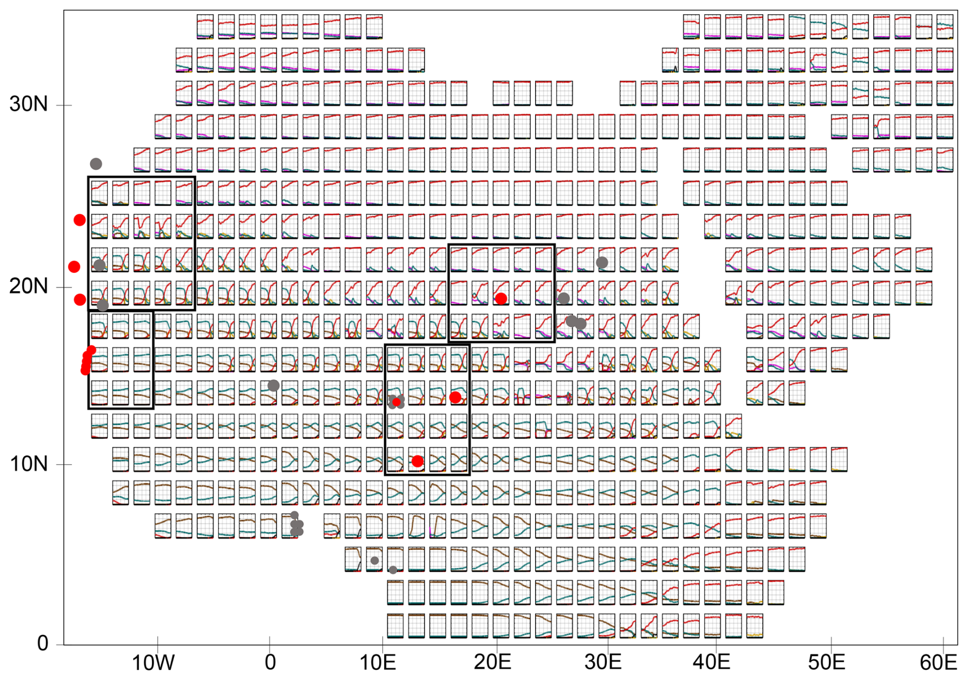
Figure A1Overview of all land grid boxes of Africa north of the Equator and Arabia in the transient MPI-ESM Holocene simulation. Shown are simulated fractions of bare surface (red lines), grass (green), shrub (purple), tropical evergreen tree (dark brown), tropical deciduous tree (light brown), and anthropogenic land cover change (black) as function of time (x-axis) between 6000 BCE and 1850 CE . The annual data are smoothed by using a 500-year Butterworth filter. The red and grey dots indicate the approximate location of marine records and pollen records in the model grid. Only the records marked by a red dot are used in the abruptness analysis, because the other records, marked by a grey dot, are too short or are located outside the area of interest. The black boxes depict the grid boxes which are used for the detailed discussion in Sect. 3. The locations of the marine and terrestrial records are listed in the Table A1.
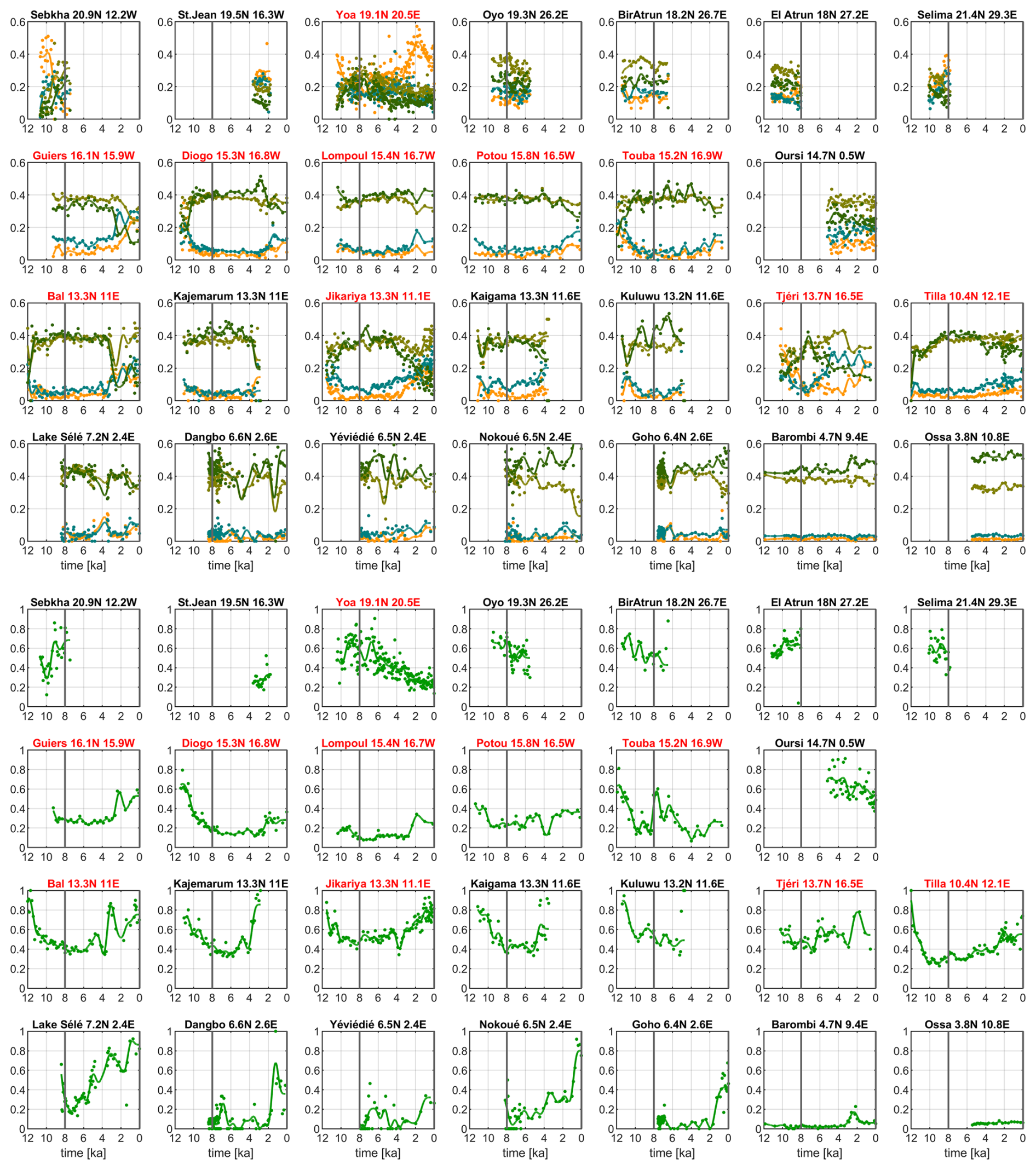
Figure A2Overview of the changing proportions of the phytogeographical groups (upper figures) and the percentage of Poaceae (lower figures) over the last 12 000 years derived from records of the African Pollen Database (Table A1). Dark green color refers to Guinean taxa, olive-green to Sudanian taxa, blue-green to Sahelian taxa, and dark yellow to Saharan taxa. The vertical grey line indicates the year 6 ka, i.e. the start of the time period of analysis. The order of records and boxes basically follows the order of their location in terms of latitude from north to south and longitude from west to east. All sites in the African Pollen Data Base for the Saharan and Sahel regions are shown. For the changepoint analysis, only records covering the last 8000 years in today's Sahara and Sahel region, i.e., records which are located south of 30° N and north of 10° N are considered. Please note that in the upper figure, the values of the y-axes range from 0 to 0.6 and in the lower figure, from 0 to 1.
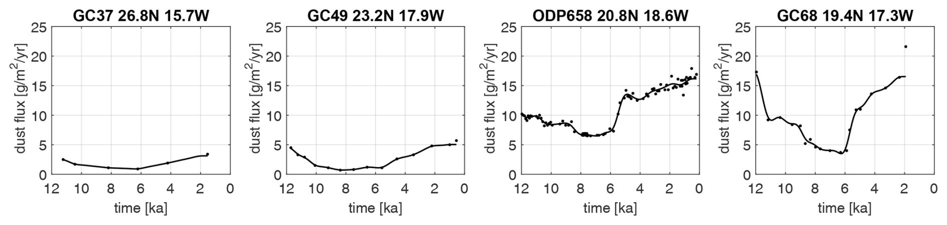
Figure A3Overview of dust flux reconstructions from marine records used for estimating total vegetation change in the western Sahara represented by the dust fluxes reconstructed from the records GC37, GC49, ODP658 and GC68 (Adkins et al., 2006; Albani et al., 2015; McGee et al., 2013). We only consider marine cores located south of 30° N. Marine cores which are located further north reveal climatic conditions and dynamics that differ from the more southerly located cores (Dallmeyer et al., 2020; Tierney et al., 2017). We also disregard the core GC37, because of its very coarse resolution.
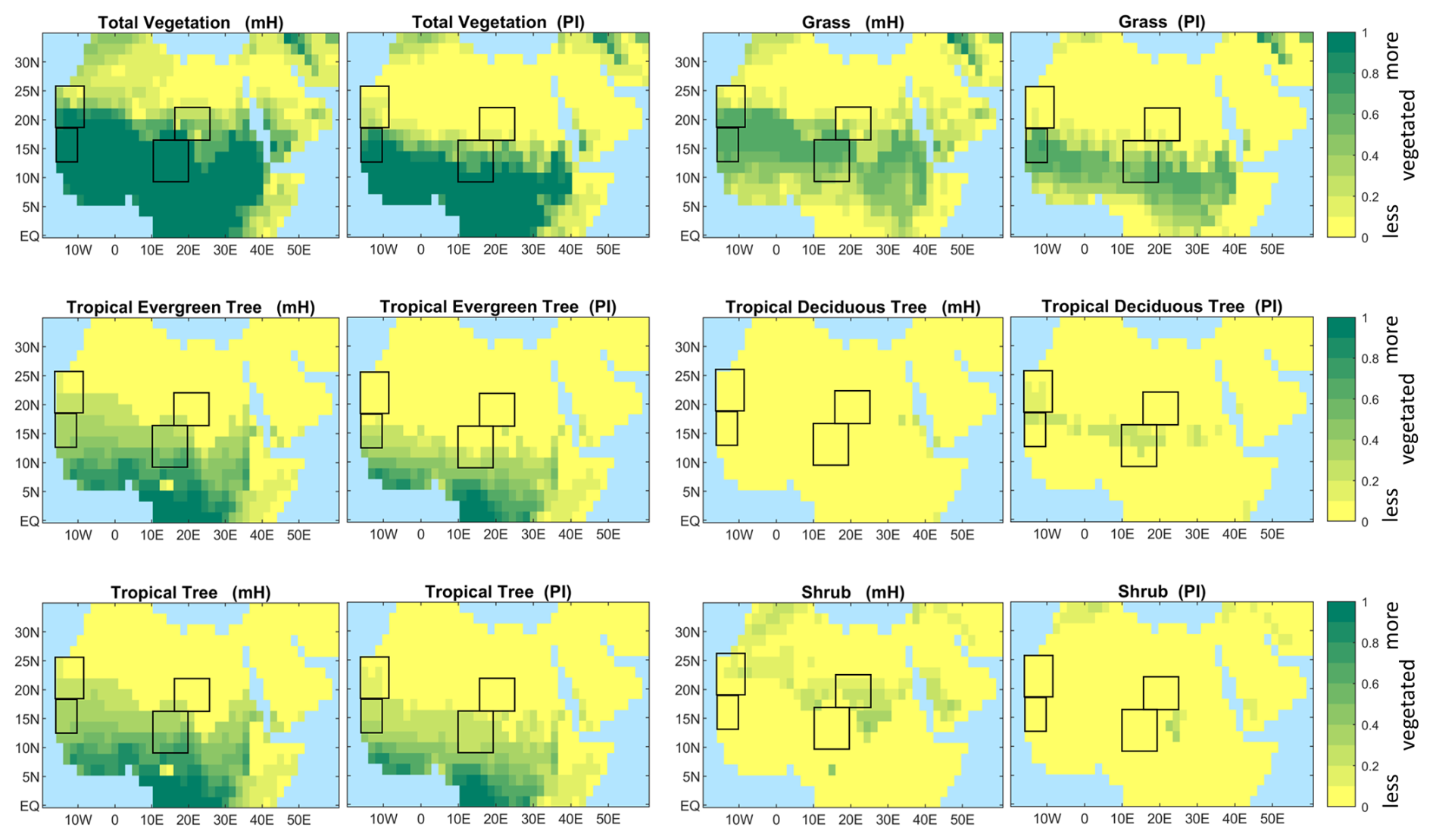
Figure A4Patterns and proportions of total vegetation cover (i.e., the complement to the bare surface fraction) and of the simulated plant functional types grass, evergreen and deciduous tropical tree, and shrub at the beginning and the end of the MPI-ESM simulation. The tropical tree PFT refers to the sum of tropical evergreen and deciduous tree. Shown are the fractional coverage of PFTs in each grid box. The proportions are the average over 100 years for the time 6000 to 5901 BCE, labelled mH, for mid Holocene, and 1751 to 1850 CE, labelled PI, for pre-industrial climate. Two grid boxes in the Adamawa Plateau at around 5° N stand out in the mH plot for tropical tree cover. Because of low mid-Holocene winter temperatures simulated at the mid Holocene in the model and the prescribed bioclimatic temperature limit, only extratropical trees can exist in this region at the mid Holocene.
Table A1Position (Lat, Long), rounded average temporal resolution (Resol), rounded temporal resolution in the vicinity of an abrupt change (Resol. at tA), type of proxy data, and reference to the paper in which the data are published.
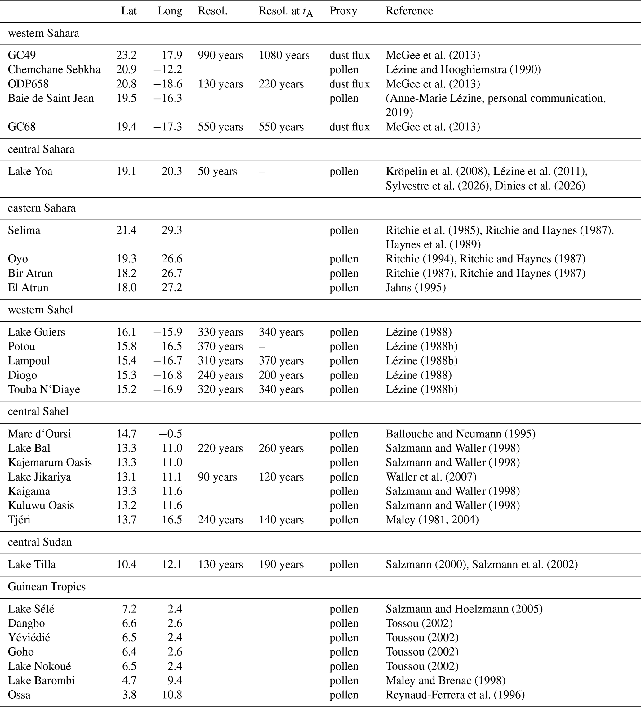
We zoom into a region in the western Sahara between some 18 to 25° N and 15 to 5° W (the upper left black box in Fig. A1) to discuss transitions in bare surface and grass PFT fraction. These reveal some peculiarities in the process description of dynamic vegetation in the land-surface model JSBACH.
The two grid boxes at around 23° N (in the third and fourth column of the second row of Fig. B1) show an apparently abrupt decrease around 6 ka followed by a more gradual increase in bare surface fraction. The rapid decrease in bare surface fraction is a consequence of the rapid increase in tropical evergreen tree fraction and grass fraction. Further analysis indicates that at the beginning of the simulation at t=8 ka, the temperature of the coldest month is below 15.5 °C, i.e., below the threshold at which tropical trees can exist. In the course of the mid Holocene, the temperature of the coldest month increases, because of the orbitally driven increase in insolation in (boreal) winter, the threshold is crossed and tropical trees can exit as shown in Fig. B2.
Thus, this bioclimatic temperature limit acts like a “tipping point” for tropical tree PFTs in our model. Due to their higher productivity, the tropical trees grow and outcompete shrub such that the tropical trees occupy the fraction of the grid box that was earlier taken by shrubs. But this is only one part of the story. Because there is enough moisture available, grass can grow which further reduces the bare surface fraction. If only shrubs and grass can exist, like in some grid boxes in the first row shown in Fig. B1, then shrubs dominate over grass. In the land-surface model JSBACH, tropical trees are not only much more productive than shrubs, but they also produce much more litter and therefore, produce more fuel for fire. And because tropical trees grow much more slowly than shrubs do, grass can grow more widespread in the presence of tropical trees (and enhanced fire activity) than in the presence of only shrubs. Finally, vegetation feeds back to climate such that a tropical tree savanna attracts more rain than a shrub savanna. The latter feature of our dynamic vegetation model is discussed in more detail in Groner et al. (2018) for equilibrium climate simulations. Here, we see the processes at work in a transient simulation.
The rapid transition from tropical evergreen to tropical deciduous tree PFT seen in the two grid boxes mentioned above (Fig. B1) is not triggered by a prescribed bioclimatic limit, but can be attributed to the simulated internal competition between tropical tree types. With increasing aridity, the deciduous tree type has an advantage over the evergreen tree type, because the allocation of carbon into leaves needs more energy than simply dropping the leaves and thereby storing the carbon into stems and roots. However, we suspect that such a transition between tropical evergreen and tropical deciduous tree is realistic. At least it is strongly model dependent. Moreover, the different taxa, Guinean, Sudanian and Sahelian, do not strictly differ by the existence or non-existence of evergreen versus deciduous trees.
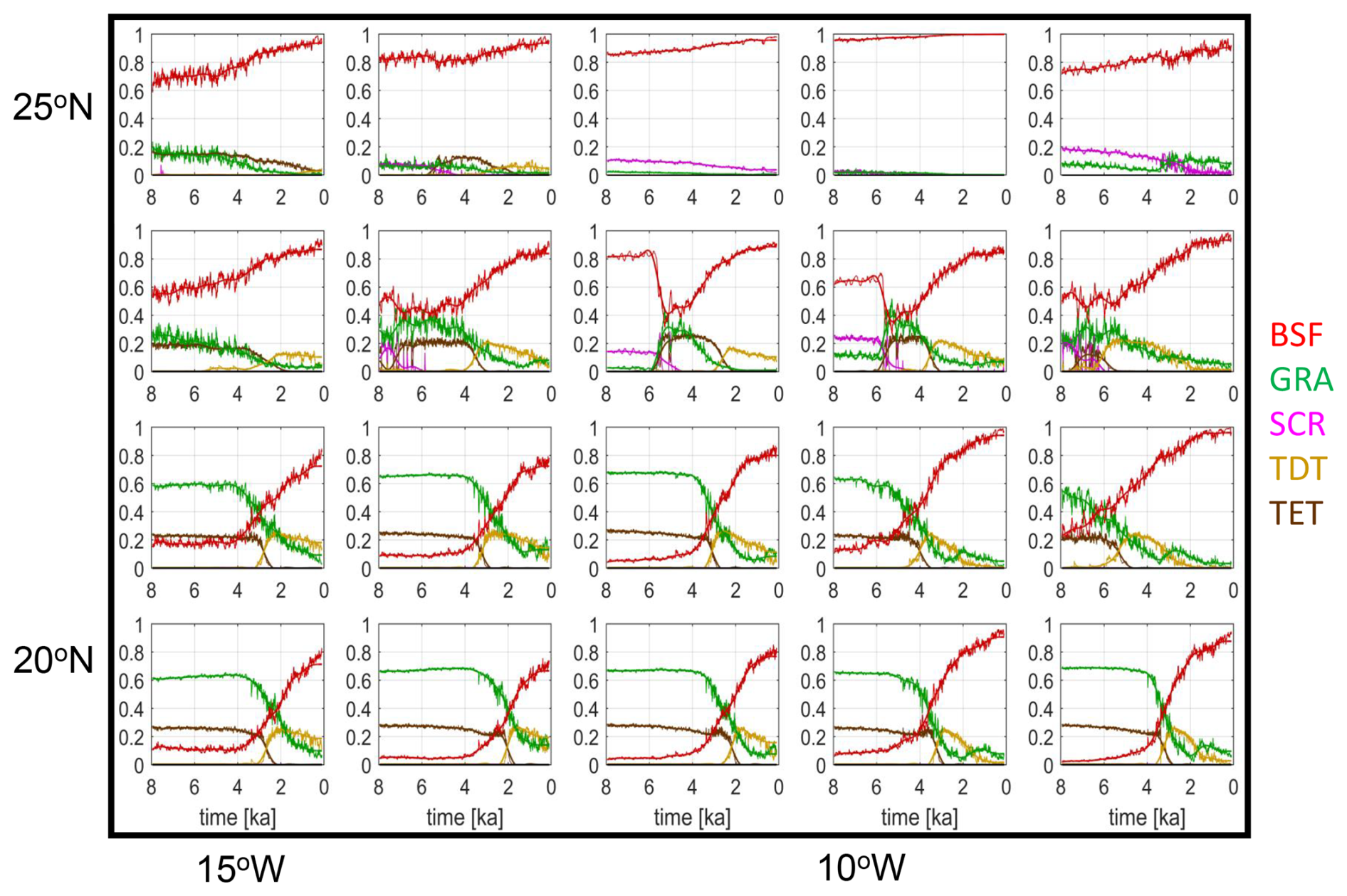
Figure B1Zoom into simulated fractions [0...1] of bare surface (red), grass PFT (blue-green), shrub PFT (magenta), tropical deciduous tree PFT (light brown) and tropical evergreen tree PFT (dark brown) as function of time between 8 ka and pre-industrial climate in the western Sahara (upper left black box in Fig. A1).
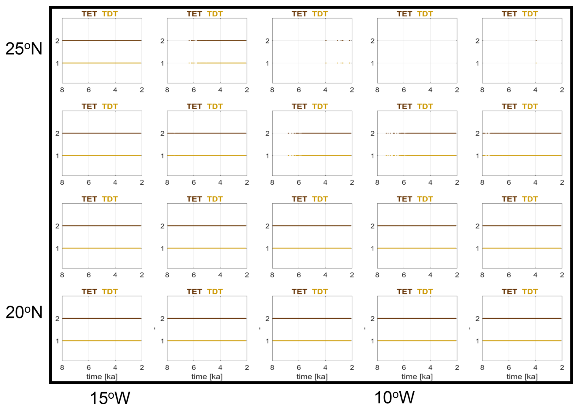
Figure B2Indication of the possible existence of tropical evergreen PFT (TET, colored dark brown) and tropical deciduous PFT (TDT, drawn in ochre). If the temperature values in a grid box are within the range of bioclimatic limits, such that a PFT can exist, then this is indicated by a dot in the sub-figures.
Table C1Time tE, the beginning of a change in a time series of pollen or dust data computed by use of the slope method proposed by Dallmeyer et al. (2020) and time tA at which the changepoint in linear regression of the time series is detected. Values in brackets indicate changepoints with a very small or with a negative offset.
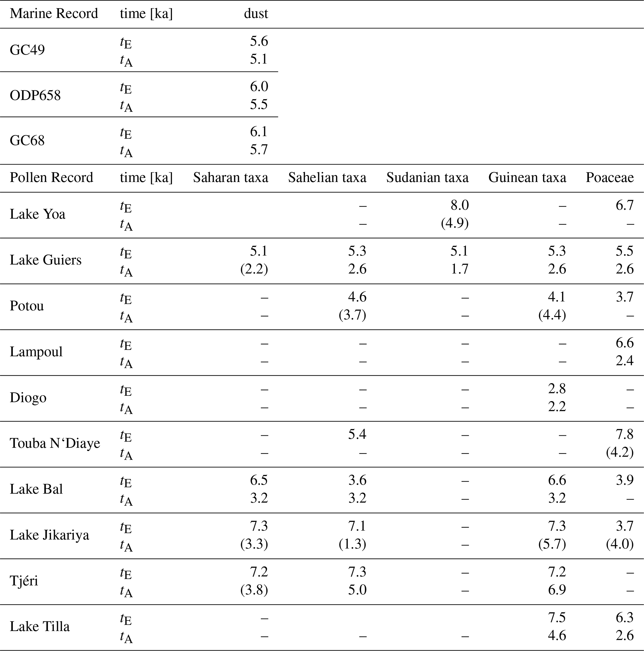
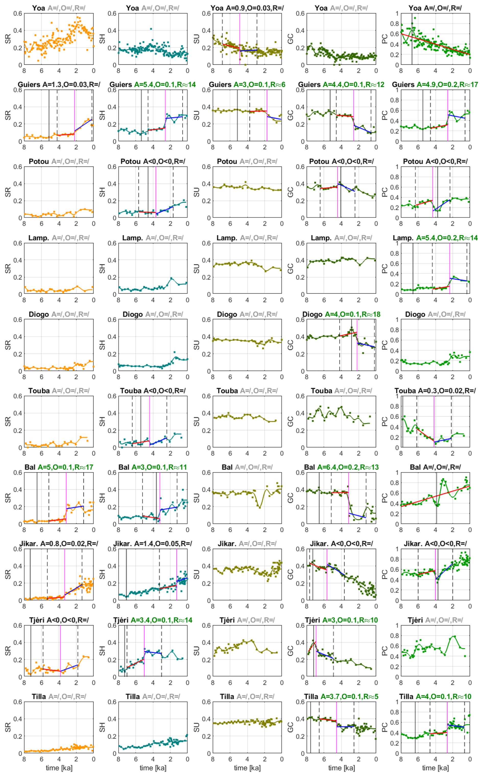
Figure C1Time series of the relative concentration of, from left to right, Saharan (SR), Sahelian (SH), Sudanian (SU), Guinean (GC) phytogeographical groups. The subplots on the far right show the relative concentration of Poaceae (PC) found in the pollen records. The title lines indicate the relative offset A (Eq. 1), the absolute offset O and the rapidity R (Eq. 3) of the transition at the changepoint in linear regression. The vertical magenta line depicts the time tA of the changepoint, the vertical dashed lines mark the time interval around the changepoint which is used for the computation of A, and the vertical black line denotes the time tE. Light gray titles indicate small long-term tendencies ΔXf<0.1, dark gray titles point at time series without a changepoint or with a negative A or a small offset O<0.05. In the latter case, only one linear regression is shown.
The transient Holocene MPI-ESM simulations are described in Bader et al. (2020) and Dallmeyer et al. (2020, 2021). The primary data, i.e. the model code for the MPI-ESM, is freely available to the scientific community and can be accessed with a license (https://mpimet.mpg.de/en/science/modeling-with-icon/code-availability, last access: 24 November 2021). The secondary data, i.e., the MPI-ESM output used for the present study, the Excel files of pollen data, the MATLAB scripts for analysis and plotting and the pptx of all original figures is archived at, and freely accessible for the scientific community from https://doi.org/10.17617/3.A122WY (Claussen, 2026).
MC designed the research and wrote a first draft of the manuscript. MC and AD analyzed the simulations. MD and FC provided and analyzed the pollen data. PH discussed the potential use of other proxy data, particularly the lake-level data. All authors discussed the results and contributed to the manuscript.
At least one of the (co-)authors is a member of the editorial board of Climate of the Past. The peer-review process was guided by an independent editor, and the authors also have no other competing interests to declare.
Publisher's note: Copernicus Publications remains neutral with regard to jurisdictional claims made in the text, published maps, institutional affiliations, or any other geographical representation in this paper. The authors bear the ultimate responsibility for providing appropriate place names. Views expressed in the text are those of the authors and do not necessarily reflect the views of the publisher.
This article is part of the special issue “Understanding past climate variability to enhance future climate-change projections (ESD/CP inter-journal SI)”. It is not associated with a conference.
The authors thank Victor Brovkin, MPI Meteorologie, Hamburg, for the helpful and constructive discussion. The constructive comments by the reviewer Jed Kaplan, an anonymous reviewer and the editor, Gerrit Lohmann, are highly appreciated.
This work contributes to the project PalMod, funded by the German Federal Ministry of Education and Research (BMBF), Research for Sustainability initiative (FONA, http://www.fona.de, last access: 24 November 2021). Anne Dallmeyer is financed by PalMod Phase III (grant no. 01LP2306A) and by the project HESCOR” funded by the program “Profilbildung 2022”, an initiative of the Ministry of Culture and Science of the State of North-Rhine Westphalia, Germany (grant no. HESCOR PB22-081). Michèle Dinies is funded by the DFG Priority Programme SPP 2143 “Entangled Africa” (project no. 404354295). Martin Claussen appreciates the funding of the Emeritus Working Group on Climate Vegetation Dynamics by the Max Planck Society.
The article processing charges for this open-access publication were covered by the Max Planck Society.
This paper was edited by Gerrit Lohmann and reviewed by Jed Kaplan and one anonymous referee.
Adkins, J., deMenocal, P., and Eshel, G.: The “African humid period” and the record of marine upwelling from excess230 Th in Ocean Drilling Program Hole 658C, Paleoceanography, 21, 2005PA001200, https://doi.org/10.1029/2005PA001200, 2006.
Albani, S., Mahowald, N. M., Winckler, G., Anderson, R. F., Bradtmiller, L. I., Delmonte, B., François, R., Goman, M., Heavens, N. G., Hesse, P. P., Hovan, S. A., Kang, S. G., Kohfeld, K. E., Lu, H., Maggi, V., Mason, J. A., Mayewski, P. A., McGee, D., Miao, X., Otto-Bliesner, B. L., Perry, A. T., Pourmand, A., Roberts, H. M., Rosenbloom, N., Stevens, T., and Sun, J.: Twelve thousand years of dust: the Holocene global dust cycle constrained by natural archives, Clim. Past, 11, 869–903, https://doi.org/10.5194/cp-11-869-2015, 2015.
Almásy, L. E.: Schwimmer in der Wüste: auf der Suche nach der Oase Zarzura Neuauflage des Werks “Unbekannte Sahara” von 1939, Neuauflage des Werks “Unbekannte Sahara” von 1939 mit... ergänzenden Kapiteln aus der ungarischen Ausgabe von 1934 sowie einem Geheimdokument über Almásys Operation Salam von 1942, Haymon, Innsbruck, ISBN: 3-85218-248-4, 1997.
Bader, J., Jungclaus, J., Krivova, N., Lorenz, S., Maycock, A., Raddatz, T., Schmidt, H., Toohey, M., Wu, C.-J., and Claussen, M.: Global temperature modes shed light on the Holocene temperature conundrum, Nat. Commun., 11, 4726, https://doi.org/10.1038/s41467-020-18478-6, 2020.
Ballouche, A. and Neumann, K.: A new contribution to the Holocene vegetation history of the West African Sahel: pollen from Oursi, Burkina Faso and charcoal from three sites in northeast Nigeria, Veg. Hist. Archaeobotany, 4, https://doi.org/10.1007/BF00198613, 1995.
Bathiany, S., Hidding, J., and Scheffer, M.: Edge Detection Reveals Abrupt and Extreme Climate Events, J. Clim., 33, 6399–6421, https://doi.org/10.1175/JCLI-D-19-0449.1, 2020.
Brierley, C., Manning, K., and Maslin, M.: Pastoralism may have delayed the end of the green Sahara, Nat. Commun., 9, 4018, https://doi.org/10.1038/s41467-018-06321-y, 2018.
Brovkin, V., Claussen, M., Petoukhov, V., and Ganopolski, A.: On the stability of the atmosphere-vegetation system in the Sahara/Sahel region, J. Geophys. Res.-Atmos., 103, 31613–31624, https://doi.org/10.1029/1998JD200006, 1998.
Brovkin, V., Raddatz, T., Reick, C. H., Claussen, M., and Gayler, V.: Global biogeophysical interactions between forest and climate, Geophys. Res. Lett., 36, 2009GL037543, https://doi.org/10.1029/2009GL037543, 2009.
Brovkin, V., Brook, E., Williams, J. W., Bathiany, S., Lenton, T. M., Barton, M., DeConto, R. M., Donges, J. F., Ganopolski, A., McManus, J., Praetorius, S., De Vernal, A., Abe-Ouchi, A., Cheng, H., Claussen, M., Crucifix, M., Gallopín, G., Iglesias, V., Kaufman, D. S., Kleinen, T., Lambert, F., Van Der Leeuw, S., Liddy, H., Loutre, M.-F., McGee, D., Rehfeld, K., Rhodes, R., Seddon, A. W. R., Trauth, M. H., Vanderveken, L., and Yu, Z.: Past abrupt changes, tipping points and cascading impacts in the Earth system, Nat. Geosci., 14, 550–558, https://doi.org/10.1038/s41561-021-00790-5, 2021.
Claussen, M.: Data related to “How abruptly did the Holocene Green Sahara end?” (1.0), Edmond [data set/code], https://doi.org/10.17617/3.A122WY, 2026.
Claussen, M., Kubatzki, C., Brovkin, V., Ganopolski, A., Hoelzmann, P., and Pachur, H.: Simulation of an abrupt change in Saharan vegetation in the Mid-Holocene, Geophys. Res. Lett., 26, 2037–2040, https://doi.org/10.1029/1999GL900494, 1999.
Claussen, M., Brovkin, V., Ganopolski, A., Kubatzki, C., and Petoukhov, V.: Climate Change in Northern Africa: The Past is Not the Future, Clim. Change, 57, 99–118, https://doi.org/10.1023/A:1022115604225, 2003.
Claussen, M., Dallmeyer, A., and Bader, J.: Theory and Modeling of the African Humid Period and the Green Sahara, Oxford University Press, https://doi.org/10.1093/acrefore/9780190228620.013.532, 2017.
D'Agostino, R., Bader, J., Bordoni, S., Ferreira, D., and Jungclaus, J.: Northern Hemisphere Monsoon Response to Mid-Holocene Orbital Forcing and Greenhouse Gas-Induced Global Warming, Geophys. Res. Lett., 46, 1591–1601, https://doi.org/10.1029/2018GL081589, 2019.
Dallmeyer, A., Claussen, M., Lorenz, S. J., and Shanahan, T.: The end of the African humid period as seen by a transient comprehensive Earth system model simulation of the last 8000 years, Clim. Past, 16, 117–140, https://doi.org/10.5194/cp-16-117-2020, 2020.
Dallmeyer, A., Claussen, M., Lorenz, S. J., Sigl, M., Toohey, M., and Herzschuh, U.: Holocene vegetation transitions and their climatic drivers in MPI-ESM1.2, Clim. Past, 17, 2481–2513, https://doi.org/10.5194/cp-17-2481-2021, 2021.
deMenocal, P., Ortiz, J., Guilderson, T., Adkins, J., Sarnthein, M., Baker, L., and Yarusinsky, M.: Abrupt onset and termination of the African Humid Period, Quat. Sci. Rev., 19, 347–361, https://doi.org/10.1016/S0277-3791(99)00081-5, 2000.
Dinerstein, E., Olson, D., Joshi, A., Vynne, C., Burgess, N. D., Wikramanayake, E., Hahn, N., Palminteri, S., Hedao, P., Noss, R., Hansen, M., Locke, H., Ellis, E. C., Jones, B., Barber, C. V., Hayes, R., Kormos, C., Martin, V., Crist, E., Sechrest, W., Price, L., Baillie, J. E. M., Weeden, D., Suckling, K., Davis, C., Sizer, N., Moore, R., Thau, D., Birch, T., Potapov, P., Turubanova, S., Tyukavina, A., De Souza, N., Pintea, L., Brito, J. C., Llewellyn, O. A., Miller, A. G., Patzelt, A., Ghazanfar, S. A., Timberlake, J., Klöser, H., Shennan-Farpón, Y., Kindt, R., Lillesø, J.-P. B., Van Breugel, P., Graudal, L., Voge, M., Al-Shammari, K. F., and Saleem, M.: An Ecoregion-Based Approach to Protecting Half the Terrestrial Realm, BioScience, 67, 534–545, https://doi.org/10.1093/biosci/bix014, 2017.
Dinies, M., Hoelzmann, P., Lebamda, J., Razanatsoa, E., Wotzka, H.-P., and Darius, F.: Ecological shifts from the Sahara to the Tropical rain forest: The past 6,000 years, in: Entangled Africa, 189–219, https://doi.org/10.34780/42s5am91, 2026.
Duffin, K. I. and Bunting, M. J.: Relative pollen productivity and fall speed estimates for southern African savanna taxa, Veg. Hist. Archaeobotany, 17, 507–525, https://doi.org/10.1007/s00334-007-0101-2, 2008.
Duque-Villegas, M., Claussen, M., Brovkin, V., and Kleinen, T.: Effects of orbital forcing, greenhouse gases and ice sheets on Saharan greening in past and future multi-millennia, Clim. Past, 18, 1897–1914, https://doi.org/10.5194/cp-18-1897-2022, 2022.
Egerer, S., Claussen, M., Reick, C., and Stanelle, T.: The link between marine sediment records and changes in Holocene Saharan landscape: simulating the dust cycle, Clim. Past, 12, 1009–1027, https://doi.org/10.5194/cp-12-1009-2016, 2016.
Egerer, S., Claussen, M., and Reick, C.: Rapid increase in simulated North Atlantic dust deposition due to fast change of northwest African landscape during the Holocene, Clim. Past, 14, 1051–1066, https://doi.org/10.5194/cp-14-1051-2018, 2018.
Eglinton, T. I., Eglinton, G., Dupont, L., Sholkovitz, E. R., Montluçon, D., and Reddy, C. M.: Composition, age, and provenance of organic matter in NW African dust over the Atlantic Ocean, Geochem. Geophys. Geosyst., 3, 1–27, https://doi.org/10.1029/2001GC000269, 2002.
Francus, P., Von Suchodoletz, H., Dietze, M., Donner, R. V., Bouchard, F., Roy, A., Fagot, M., Verschuren, D., and Kröpelin, S.: Varved sediments of Lake Yoa (Ounianga Kebir, Chad) reveal progressive drying of the Sahara during the last 6100 years, Sedimentology, 60, 911–934, https://doi.org/10.1111/j.1365-3091.2012.01370.x, 2013.
Gaillard, M.-J., Githumbi, E., Achoundong, G., Lézine, A.-M., Hély, C., Lebamba, J., Marquer, L., Mazier, F., Li, F., and Sugita, S.: The challenge of pollen-based quantitative reconstruction of Holocene plant cover in tropical regions: A pilot study in Cameroon, in: Quaternary Vegetation Dynamics – The African Pollen Database, CRC Press, London, 183–206, https://doi.org/10.1201/9781003162766-12, 2021.
Gajewski, K., Lézine, A.-M., Vincens, A., Delestan, A., and Sawada, M.: Modern climate–vegetation–pollen relations in Africa and adjacent areas, Quat. Sci. Rev., 21, 1611–1631, https://doi.org/10.1016/S0277-3791(01)00152-4, 2002.
Groner, V. P., Raddatz, T., Reick, C. H., and Claussen, M.: Plant functional diversity affects climate–vegetation interaction, Biogeosciences, 15, 1947–1968, https://doi.org/10.5194/bg-15-1947-2018, 2018.
Haynes, C. V., Eyles, C. H., Pavlish, L. A., Ritchie, J. C., and Rybak, M.: Holocene palaeoecology of the eastern Sahara; Selima Oasis, Quat. Sci. Rev., 8, 109–136, https://doi.org/10.1016/0277-3791(89)90001-2, 1989.
Hély, C., Lézine, A.-M., and contributors, A.: Holocene changes in African vegetation: tradeoff between climate and water availability, Clim. Past, 10, 681–686, https://doi.org/10.5194/cp-10-681-2014, 2014.
Higgins, S. I. and Scheiter, S.: Atmospheric CO2 forces abrupt vegetation shifts locally, but not globally, Nature, 488, 209–212, https://doi.org/10.1038/nature11238, 2012.
Hill, T. R., Duthie, T. J., and Bunting, J.: Pollen productivity estimates from KwaZulu-Natal Drakensberg, South Africa, in: Quaternary Vegetation Dynamics – The African Pollen Database, CRC Press, London, 259–274, https://doi.org/10.1201/9781003162766-16, 2021.
Hoelzmann, P., Gasse, F., Dupont, L. M., Salzmann, U., Staubwasser, M., Leuschner, D. C., and Sirocko, F.: Palaeoenvironmental changes in the arid and sub arid belt (Sahara-Sahel-Arabian Peninsula) from 150 kyr to present, in: Past Climate Variability through Europe and Africa, vol. 6, edited by: Battarbee, R. W., Gasse, F., and Stickley, C. E., Springer Netherlands, Dordrecht, 219–256, https://doi.org/10.1007/978-1-4020-2121-3_12, 2004.
Holmes, J. and Hoelzmann, P.: The Late Pleistocene-Holocene African Humid Period as Evident in Lakes, Oxford University Press, https://doi.org/10.1093/acrefore/9780190228620.013.531, 2017.
Hopcroft, P. O. and Valdes, P. J.: Paleoclimate-conditioning reveals a North Africa land–atmosphere tipping point, Proc. Natl. Acad. Sci. USA, 118, e2108783118, https://doi.org/10.1073/pnas.2108783118, 2021.
Hopcroft, P. O. and Valdes, P. J.: Green Sahara tipping points in transient climate model simulations of the Holocene, Environ. Res. Lett., 17, 085001, https://doi.org/10.1088/1748-9326/ac7c2b, 2022.
Hurtt, G. C., Chini, L., Sahajpal, R., Frolking, S., Bodirsky, B. L., Calvin, K., Doelman, J. C., Fisk, J., Fujimori, S., Klein Goldewijk, K., Hasegawa, T., Havlik, P., Heinimann, A., Humpenöder, F., Jungclaus, J., Kaplan, J. O., Kennedy, J., Krisztin, T., Lawrence, D., Lawrence, P., Ma, L., Mertz, O., Pongratz, J., Popp, A., Poulter, B., Riahi, K., Shevliakova, E., Stehfest, E., Thornton, P., Tubiello, F. N., van Vuuren, D. P., and Zhang, X.: Harmonization of global land use change and management for the period 850–2100 (LUH2) for CMIP6, Geosci. Model Dev., 13, 5425–5464, https://doi.org/10.5194/gmd-13-5425-2020, 2020.
Jahns, S.: A Holocene pollen diagram from El Atrun, northern Sudan, Veg. Hist. Archaeobotany, 4, 23–30, 1995.
Julier, A. C. M., Jardine, P. E., Adu-Bredu, S., Coe, A. L., Duah-Gyamfi, A., Fraser, W. T., Lomax, B. H., Malhi, Y., Moore, S., Owusu-Afriyie, K., and Gosling, W. D.: The modern pollen–vegetation relationships of a tropical forest–savannah mosaic landscape, Ghana, West Africa, Palynology, 42, 324–338, https://doi.org/10.1080/01916122.2017.1356392, 2018.
Kröpelin, S., Verschuren, D., Lézine, A.-M., Eggermont, H., Cocquyt, C., Francus, P., Cazet, J.-P., Fagot, M., Rumes, B., Russell, J. M., Darius, F., Conley, D. J., Schuster, M., Von Suchodoletz, H., and Engstrom, D. R.: Climate-Driven Ecosystem Succession in the Sahara: The Past 6000 Years, Science, 320, 765–768, https://doi.org/10.1126/science.1154913, 2008.
Kuper, R. and Kröpelin, S.: Climate-Controlled Holocene Occupation in the Sahara: Motor of Africa's Evolution, Science, 313, 803–807, https://doi.org/10.1126/science.1130989, 2006.
Le Houérou, H.-N.: Définition et limites bioclimatiques du Sahara, Sci. Chang. Planétaires Sécher., 1, 246–259, 1990.
Lemmonier, K. and Lézine, A.-M.: Timing and nature of the end of the African Humid Period in the Sahel: insight from pollen data, Palaeoecol. Afr., 35, 51–64, 2022.
Lézine, A.-M.: New pollen data from the Sahel, Senegal, Rev. Palaeobot. Palynol., 55, 141–154, https://doi.org/10.1016/0034-6667(88)90082-6, 1988a.
Lézine, A.-M.: Les variations de la couverture forestière mésophile d'Afrique occidentale au cours de l'Holocène, Comptes Rendus Académie Sci. Sér. II Mech. Phys. Chem. Space Sci. Earth Sci., 307, 439–445, 1988b.
Lézine, A.-M. and Edorh, T. M.: Modern pollen deposition in West African Sudanian environments, Rev. Palaeobot. Palynol., 67, 41–58, https://doi.org/10.1016/0034-6667(91)90015-U, 1991.
Lézine, A.-M. and Hooghiemstra, H.: Land-sea comparisons during the last glacial-interglacial transition: pollen records from West Tropical Africa, Palaeogeogr. Palaeoclimatol. Palaeoecol., 79, 313–331, https://doi.org/10.1016/0031-0182(90)90025-3, 1990.
Lézine, A.-M., Hély, C., Grenier, C., Braconnot, P., and Krinner, G.: Sahara and Sahel vulnerability to climate changes, lessons from Holocene hydrological data, Quat. Sci. Rev., 30, 3001–3012, https://doi.org/10.1016/j.quascirev.2011.07.006, 2011.
Linder, P., Lovett, J., Mutke, J., Barthlott, W., Jürgens, J., Rebelo, T., and Küper, W.: A numerical re-evaluation of the sub-Saharan Phytochoria of mainland Africa, Biol. Skr., 55, 229–252, 2005.
Liu, Z., Wang, Y., Gallimore, R., Notaro, M., and Prentice, I. C.: On the cause of abrupt vegetation collapse in North Africa during the Holocene: Climate variability vs. vegetation feedback, Geophys. Res. Lett., 33, 2006GL028062, https://doi.org/10.1029/2006GL028062, 2006.
Maley, J.: La sédimentation pollinique actuelle dans la zone du Lac Tchad (Afrique centrale), Pollen Spores, 14, 264–307, 1972.
Maley, J.: Mecanisme des changements climatiques aux basses latitudes, Palaeogeogr. Palaeoclimatol. Palaeoecol., 14, 193–227, https://doi.org/10.1016/0031-0182(73)90003-5, 1973.
Maley, J.: Etudes palynologiques dans le bassin du Tchad et paléoclimatologie de l'Afrique Nord-Tropicale de 30.000 ans à l'époque actuelle, Trav. Doc., 129, 586 p., ISBN: 2-7099-0592-2, 1981.
Maley, J.: Le bassin du Tchad au Quaternaire récent: formations sédimentaires, paléoenvironnements et préhistoire. La question des Paléotchads, Evol. Végétation Depuis Deux Millions D'années Errance, ISBN: 2-87772-278-3, 2004.
Maley, J. and Brenac, P.: Vegetation dynamics, palaeoenvironments and climatic changes in the forests of western Cameroon during the last 28,000 years B.P., Rev. Palaeobot. Palynol., 99, 157–187, https://doi.org/10.1016/S0034-6667(97)00047-X, 1998.
Mauritsen, T., Bader, J., Becker, T., Behrens, J., Bittner, M., Brokopf, R., Brovkin, V., Claussen, M., Crueger, T., Esch, M., Fast, I., Fiedler, S., Fläschner, D., Gayler, V., Giorgetta, M., Goll, D. S., Haak, H., Hagemann, S., Hedemann, C., Hohenegger, C., Ilyina, T., Jahns, T., Jimenéz-de-la-Cuesta, D., Jungclaus, J., Kleinen, T., Kloster, S., Kracher, D., Kinne, S., Kleberg, D., Lasslop, G., Kornblueh, L., Marotzke, J., Matei, D., Meraner, K., Mikolajewicz, U., Modali, K., Möbis, B., Müller, W. A., Nabel, J. E. M. S., Nam, C. C. W., Notz, D., Nyawira, S., Paulsen, H., Peters, K., Pincus, R., Pohlmann, H., Pongratz, J., Popp, M., Raddatz, T. J., Rast, S., Redler, R., Reick, C. H., Rohrschneider, T., Schemann, V., Schmidt, H., Schnur, R., Schulzweida, U., Six, K. D., Stein, L., Stemmler, I., Stevens, B., Von Storch, J., Tian, F., Voigt, A., Vrese, P., Wieners, K., Wilkenskjeld, S., Winkler, A., and Roeckner, E.: Developments in the MPI-M Earth System Model version 1.2 (MPI-ESM1.2) and Its Response to Increasing CO2, J. Adv. Model. Earth Syst., 11, 998–1038, https://doi.org/10.1029/2018MS001400, 2019.
McGee, D., deMenocal, P. B., Winckler, G., Stuut, J. B. W., and Bradtmiller, L. I.: The magnitude, timing and abruptness of changes in North African dust deposition over the last 20,000 yr, Earth Planet. Sci. Lett., 371–372, 163–176, https://doi.org/10.1016/j.epsl.2013.03.054, 2013.
Olson, D. M., Dinerstein, E., Wikramanayake, E. D., Burgess, N. D., Powell, G. V. N., Underwood, E. C., D'amico, J. A., Itoua, I., Strand, H. E., Morrison, J. C., Loucks, C. J., Allnutt, T. F., Ricketts, T. H., Kura, Y., Lamoreux, J. F., Wettengel, W. W., Hedao, P., and Kassem, K. R.: Terrestrial Ecoregions of the World: A New Map of Life on Earth, BioScience, 51, 933, https://doi.org/10.1641/0006-3568(2001)051[0933:TEOTWA]2.0.CO;2, 2001.
Pausata, F. S. R., Gaetani, M., Messori, G., Berg, A., Maia De Souza, D., Sage, R. F., and deMenocal, P. B.: The Greening of the Sahara: Past Changes and Future Implications, One Earth, 2, 235–250, https://doi.org/10.1016/j.oneear.2020.03.002, 2020.
Phelps, L. N., Chevalier, M., Shanahan, T. M., Aleman, J. C., Courtney-Mustaphi, C. J., Kiahtipes, C. A., Broennimann, O., Marchant, R., Shekeine, J., Quick, L. J., Davis, B. A. S., Metwally, A. A., Bamford, M., Neuman, F. H., Scott, L., Cordova, C., Burrough, S. L., Manning, K., and Guisan, A.: Pollen dataset for “Asymmetric response of forest and grassy biomes to climate variability across the African Humid Period: influenced by anthropogenic disturbance?,” PANGAEA [data set], https://doi.org/10.1594/PANGAEA.905309, 2019.
Quézel, P.: La végétation du Sahara, Gustav Fischer, Stuttgart, 333 pp., 1965.
Reick, C. H., Raddatz, T., Brovkin, V., and Gayler, V.: Representation of natural and anthropogenic land cover change in MPI-ESM, J. Adv. Model. Earth Syst., 5, 459–482, https://doi.org/10.1002/jame.20022, 2013.
Reick, C. H., Gayler, V., Goll, D., Hagemann, S., Heidkamp, M., Nabel, J. E. M. S., Raddatz, T., Roeckner, E., Schnur, R., and Wilkenskjeld, S.: JSBACH 3 – The land component of the MPI Earth System Model: documentation of version 3.2, 4990986, https://doi.org/10.17617/2.3279802, 2021.
Reynaud-Farrera, I., Maley, J., and Wirrmann, D.: Végétation et climat dans les forêts du Sud-Ouest Cameroun depuis 4770 ans BP: analyse pollinique des sédiments du Lac Ossa, CR Acad Sci Paris, 322, 749–755, https://www.researchgate.net/publication/32970399 (last access: 12 November 2026), 1996.
Ritchie, J. C.: A Holocene pollen record from Bir Atrun, northwest Sudan, Pollen Spores, 29, 391–410, 1987.
Ritchie, J. C.: Holocene pollen spectra from Oyo, northwestern Sudan: problems of interpretation in a hyperarid environment, The Holocene, 4, 9–15, https://doi.org/10.1177/095968369400400102, 1994.
Ritchie, J. C. and Haynes, C. V.: Holocene vegetation zonation in the eastern Sahara, Nature, 330, 645–647, https://doi.org/10.1038/330645a0, 1987.
Ritchie, J. C., Eyles, C. H., and Haynes, C. V.: Sediment and pollen evidence for an early to mid-Holocene humid period in the eastern Sahara, Nature, 314, 352–355, https://doi.org/10.1038/314352a0, 1985.
Rossignol-Strick, M.: Mediterranean Quaternary sapropels, an immediate response of the African monsoon to variation of insolation, Palaeogeogr. Palaeoclimatol. Palaeoecol., 49, 237–263, 1985.
Salzmann, U.: Pollenanalytical studies in NE-Nigeria: preliminary results from the Manga Grasslands and Lake Tilla, Biu Plateau, Berichte Sonderforschungsbereiches 268, 8, https://d-nb.info/1222462036/34 (last access: 12 October 2026), 1996.
Salzmann, U.: Are modern savannas degraded forests? – A Holocene pollen record from the Sudanian vagetation zone of NE Nigeria, Veg. Hist. Archaeobotany, 9, 1–15, https://doi.org/10.1007/BF01295010, 2000.
Salzmann, U. and Hoelzmann, P.: The Dahomey Gap: an abrupt climatically induced rain forest fragmentation in West Africa during the late Holocene, The Holocene, 15, 190–199, https://doi.org/10.1191/0959683605hl799rp, 2005.
Salzmann, U. and Waller, M.: The Holocene vegetational history of the Nigerian Sahel based on multiple pollen profiles, Rev. Palaeobot. Palynol., 100, 39–72, https://doi.org/10.1016/S0034-6667(97)00053-5, 1998.
Salzmann, U., Hoelzmann, P., and Morczinek, I.: Late Quaternary Climate and Vegetation of the Sudanian Zone of Northeast Nigeria, Quat. Res., 58, 73–83, https://doi.org/10.1006/qres.2002.2356, 2002.
Sayre, R. G., Comer, P., Hak, J., Josse, C., Bow, J., Warner, H., Larwanou, M., Kelbessa, E., Bekele, T., Kehl, H., Amena, R., Andriamasimanana, R., Ba, T., Benson, L., Boucher, T., Brown, M., Cress, J. J., Dassering, O., Friesen, B. A., Gachathi, F., Houcine, S., Keita, M., Khamala, E., Marangu, D., Mokua, F., Morou, B., Mucina, L., Mugisha, S., Mwavu, E., Rutherford, M., Sanou, P., Syampungani, S., Tomor, B., Vall, A. O. M., Vande Weghe, J. P., Wangui, E., and Waruingi, L.: A new map of standardized terrestrial ecosystems of Africa, African Geographical Review, https://ui.adsabs.harvard.edu/abs/2013agr..rept.....S (last access: 31 March 2026), 2013.
Scheiter, S., Moncrieff, G. R., Pfeiffer, M., and Higgins, S. I.: African biomes are most sensitive to changes in CO2 under recent and near-future CO2 conditions, Biogeosciences, 17, 1147–1167, https://doi.org/10.5194/bg-17-1147-2020, 2020.
Schulz, E.: Zwischen Syrte und Tschad. Der aktuelle Pollenniederschlag in der Sahara, Berl. Geogr. Stud., 30, ISSN: 0341-8537, 1990.
Shanahan, T. M., McKay, N. P., Hughen, K. A., Overpeck, J. T., Otto-Bliesner, B., Heil, C. W., King, J., Scholz, C. A., and Peck, J.: The time-transgressive termination of the African Humid Period, Nat. Geosci., 8, 140–144, https://doi.org/10.1038/ngeo2329, 2015.
Specht, N. F., Claussen, M., and Kleinen, T.: Dynamic interaction between lakes, climate, and vegetation across northern Africa during the mid-Holocene, Clim. Past, 20, 1595–1613, https://doi.org/10.5194/cp-20-1595-2024, 2024.
Sylvestre, F., Melles, M., Wennrich, V., Dinies, M., Chalié, F., Swingedouw, D., Dallmeyer, A., Shi, X., Claussen, M., Jaeschke, A., Cocquyt, C., Karls, J., Kuper, J., Mallaye, B., Mazur, J.-C., Paillès, C., Rirongarti, R., Rethemeyer, J., Ritter-Prinz, B., Schefuß, E., Viehberg, F., Wagner, B., Werner, M., Yacoub, A. N., and Kröpelin, S.: Decadal-scale droughts disrupted the African Humid Period in the Sahara, Nature, https://doi.org/10.1038/s41586-026-10336-7, 2026.
Tabares, X., Ratzmann, G., Kruse, S., Theuerkauf, M., Mapani, B., and Herzschuh, U.: Relative pollen productivity estimates of savanna taxa from southern Africa and their application to reconstruct shrub encroachment during the last century, The Holocene, 31, 1100–1111, https://doi.org/10.1177/09596836211003193, 2021.
The MathWorks Inc.: MATLAB version R2018a (version 9.4.0.813654), https://www.mathworks.com (last access: 17 February 2020), 2018.
Tierney, J. E. and deMenocal, P. B.: Abrupt Shifts in Horn of Africa Hydroclimate Since the Last Glacial Maximum, Science, 342, 843–846, https://doi.org/10.1126/science.1240411, 2013.
Tierney, J. E., Pausata, F. S. R., and deMenocal, P. B.: Rainfall regimes of the Green Sahara, Sci. Adv., 3, e1601503, https://doi.org/10.1126/sciadv.1601503, 2017.
Tossou, M. G.: Recherche palynologique sur la végétation Holocène du Sud-Bénin (Afrique de l'Ouest), Thèse de doctorat, Université de Lome (Togo), 133 pp., https://d-ist.univ-lome.tg:8082/opac_css/index.php?lvl=author_see&id=16183/ (last access: 16 November 2026), 2002.
Trauth, M. H., Foerster, V., Junginger, A., Asrat, A., Lamb, H. F., and Schaebitz, F.: Abrupt or gradual? Change point analysis of the late Pleistocene–Holocene climate record from Chew Bahir, southern Ethiopia, Quat. Res., 90, 321–330, https://doi.org/10.1017/qua.2018.30, 2018.
Vincens, A., Lézine, A.-M., Buchet, G., Lewden, D., and Le Thomas, A.: African pollen database inventory of tree and shrub pollen types, Rev. Palaeobot. Palynol., 145, 135–141, https://doi.org/10.1016/j.revpalbo.2006.09.004, 2007.
Waller, M. P., Street-Perrott, F. A., and Wang, H.: Holocene vegetation history of the Sahel: pollen, sedimentological and geochemical data from Jikariya Lake, north-eastern Nigeria, J. Biogeogr., 34, 1575–1590, https://doi.org/10.1111/j.1365-2699.2007.01721.x, 2007.
Walter, H. and Breckle, S.-W.: Ökologie der Erde. 1: Ökologische Grundlagen in globaler Sicht, Fischer, Stuttgart, ISBN: 978-3-437-20454-8, 1991.
White, F.: The vegetation of Africa: a descriptive memoir to accompany the Unesco/AETFAT/UNSO vegetation map of Africa, Unesco, Paris, 356 pp., ISBN: 978-92-3-101955-5, 1983.
Wright, D. K.: Humans as Agents in the Termination of the African Humid Period, Front. Earth Sci., 5, https://doi.org/10.3389/feart.2017.00004, 2017.
Yu, K., D'Odorico, P., Bhattachan, A., Okin, G. S., and Evan, A. T.: Dust-rainfall feedback in West African Sahel, Geophys. Res. Lett., 42, 7563–7571, https://doi.org/10.1002/2015GL065533, 2015.
- Abstract
- Introduction
- Data and Methods
- Results
- Discussion
- Conclusions
- Appendix A: Overview of all model and pollen data
- Appendix B: Example of PFT dynamics triggered by changes in temperature
- Appendix C: Additional analysis of pollen records
- Code and data availability
- Author contributions
- Competing interests
- Disclaimer
- Special issue statement
- Acknowledgements
- Financial support
- Review statement
- References
- Abstract
- Introduction
- Data and Methods
- Results
- Discussion
- Conclusions
- Appendix A: Overview of all model and pollen data
- Appendix B: Example of PFT dynamics triggered by changes in temperature
- Appendix C: Additional analysis of pollen records
- Code and data availability
- Author contributions
- Competing interests
- Disclaimer
- Special issue statement
- Acknowledgements
- Financial support
- Review statement
- References