The influence of glacial Northern Hemisphere ice sheets on atmospheric circulation

The Laurentide ice-sheet affected the North Atlantic Ocean during the last glacial period, but its impact on the global atmospheric circulation remains unclear. Here, we use the Australian Earth System Model to investigate the relative roles of Marine Isotope Stage 3 (65 000–25 000 years ago; 65–25 ka) boundary conditions in shaping global climate ∼ 49 ka, a period marked by prominent millennial-scale variability. Our simulations show that Northern Hemisphere (NH) ice sheets were the primary driver of large-scale circulation changes. In particular, NH ice-sheet topography induced a 6 and 4° southward shift of the NH westerlies during boreal winter and summer, respectively, increasing rainfall over Eurasia during summer by 31 % but reducing it in winter. In contrast, orbital forcing and greenhouse gas (GHG) changes did not lead to a significant NH westerly shift, while ice-sheet albedo strengthened the NH westerlies (10 %–14 %) through enhanced cooling (by 3–4 °C) without altering their position in both seasons. NH ice-sheet topography also affected the global atmospheric circulation, leading to an additional 0.9° southward shift of the Intertropical Convergence Zone (ITCZ) and a 1.5° southward displacement of the NH Hadley cell in austral summer, relative to changes simulated due to orbital forcing plus GHG (0.6 and 2° southward shifts for the ITCZ and the NH Hadley cell, respectively), and albedo (0.4 and 0.1°, respectively). The full glacial boundary conditions, including changes in Antarctic ice-sheet topography, also led to a 2° equatorward shift of the Southern Hemisphere (SH) Hadley cell, and a 2.5° equatorward shift of the SH westerlies during austral winter. Orbital forcing plus GHG and albedo primarily modulated the strength of the SH westerlies and tropical atmospheric circulation. These results highlight the role of ice-sheet topography in controlling shifts in the atmospheric circulation and the role of surface albedo in modulating atmospheric circulation intensity through radiative cooling.

1 Introduction

Earth's climate history has been shaped by the expansion and retreat of Northern Hemisphere (NH) ice sheets, particularly during the last glacial cycle. The expansion of large NH ice sheets has long been associated with global and regional cooling, particularly over the North Atlantic, which is directly influenced by the ice sheet extent and height (Kageyama et al., 2021). Ice sheet growth affects land-ocean geography by lowering sea levels (Lambeck et al., 2014), exposing land bridges, and altering local heating patterns due to the differing heat capacities of land and ocean (Byrne and O'Gorman, 2013). Additionally, changes in land bridges and oceanic gateways, such as the Bering Strait, influence large-scale ocean circulation, including the Atlantic Meridional Overturning Circulation (AMOC) (Hu et al., 2015). These factors have significant implications for the climate system, particularly through their impact on the atmospheric circulation and ocean currents.

In today's climate, warm water in the North Atlantic is transported northward via the Gulf Stream, and atmospheric Rossby wave propagation results in a northeastward-tilted Atlantic jet stream. This configuration contributes to the relatively mild winters in Europe compared to regions at similar latitudes in North America (Seager et al., 2002; Brayshaw et al., 2009). However, during past glacial periods, and particularly the Last Glacial Maximum (LGM; 19–21 ka), thick ice sheets covered northern North America and may have reached up to 5 km in height (Peltier, 2004). This so-called Laurentide Ice Sheet (LIS) caused a pronounced southward shift of the jet stream, and in some cases, a more zonal orientation compared to today's tilted pattern (Manabe and Broccoli, 1985; Pausata et al., 2011; Löfverström et al., 2014; Ullman et al., 2014). This southward shift of the jet stream, which was primarily driven by ice sheet topography, rather than changes in albedo or greenhouse gas (GHG) forcing (Pausata et al., 2011), had important consequences for European climate, impacting winter storm tracks, precipitation, and seasonal temperatures (Löfverström et al., 2014).

Previous research on the impact of NH ice sheets on climate (Broccoli and Manabe, 1987; Pausata et al., 2011; Löfverström et al., 2014; Ullman et al., 2014; Wang et al., 2018; Izumi et al., 2023) primarily focused on the LGM, an important period due to its extreme climate conditions, including the coldest global temperatures (Kageyama et al., 2021), lowest atmospheric CO₂ levels (Köhler et al., 2017), and most extensive ice sheets (Peltier, 2004; Clark et al., 2009; Kageyama et al., 2017; Gowan et al., 2021). Most of these studies examined the North Atlantic region, assessing the impact of ice sheets on NH westerlies and the Atlantic jet, with limited investigation into regions beyond this sector. Löfverström et al. (2014) investigated both the LGM as well as pre-LGM ice sheets of Marine Isotope Stage (MIS) 5b (∼ 88 ka) and MIS 4 (∼ 66 ka) and found that the westerlies shifted southward in all ice sheet configurations, but a fully zonal jet orientation emerged only during the LGM. They also suggested that the ice sheet topography dynamically induced warming in Alaska and central Asia, potentially contributing to the westward expansion of the Eurasian ice sheets from MIS 4 to the LGM. Other studies, such as Ullman et al. (2014) and Zhang et al. (2014a), further explored the impact of different LIS heights on both the atmosphere and the ocean.

In contrast, the climate of MIS 3 (65–25 ka) has received comparatively less attention in the context of ice sheet–atmosphere interactions. Existing studies of MIS 3 have largely concentrated on large-scale oceanic responses, such as AMOC variability, surface temperature patterns, and sea ice changes (Merkel et al., 2010; Brandefelt et al., 2011; Guo et al., 2019; Malmierca-Vallet and Sime, 2023). Some have investigated tropical climate variability, including changes in El Niño–Southern Oscillation (ENSO) behaviour during this period (Brandefelt et al., 2011; Merkel et al., 2010), while others reported a southward-shifted ITCZ and associated changes in tropical precipitation and Southern Hemisphere (SH) circulation (Guo et al., 2019). However, the detailed, mechanistic impacts of NH ice sheets on atmospheric circulation during MIS 3 – particularly beyond the North Atlantic – remain underexplored. This gap may be partly due to the significant millennial-scale climate variability that characterizes MIS 3 – including abrupt temperature fluctuations in Greenland of 8–10 °C (Huber et al., 2006) and multiple episodes of AMOC weakening (Menviel et al., 2020 and references therein) – which makes it challenging to isolate the equilibrium climate response to boundary conditions. Here, we employ quasi-equilibrium climate simulations with prescribed 49 ka boundary conditions and systematically isolate the effects of orbital parameters and GHGs, ice-sheet albedo, and ice-sheet topography. This framework enables us to quantify the mechanistic contribution of each forcing to atmospheric circulation and hydroclimate changes during MIS 3.

The period around 49 ka stands out due to one of the highest obliquity values (24.43°) of the last glacial cycle (Berger, 1978), resulting in greater summer insolation in both hemispheres compared to the preindustrial (PI). Variations in obliquity alter the distribution of incoming solar radiation across latitudes at the top of the atmosphere. High obliquity increases incoming solar insolation at high latitudes in summer, while decreasing it in winter, leading to enhanced seasonal contrast with warmer summers and colder winters in both hemispheres. These changes in radiative forcing influence the large-scale atmospheric circulation and can affect the position and strength of the Hadley circulation and the ITCZ (Mantsis et al., 2014; Liu et al., 2015; Zhang et al., 2022). In particular, 49 ka exhibits an obliquity value higher than some interglacial periods, such as the Last Interglacial (LIG, 127 ka), yet features a climate state marked by low CO₂ (∼ 199 ppm, similar to LGM (Köhler et al., 2017)) and extensive Laurentide and Scandinavian ice sheets (Gowan et al., 2021), leading to a colder-than-PI climate. Furthermore, global sea levels were approximately 60–65 m lower than PI (Shakun et al., 2015). This unusual combination of strong seasonal insolation forcing, associated with high obliquity and low atmospheric CO₂ and extensive ice sheets, provides an opportunity to investigate how competing climate forcings interact to shape atmospheric teleconnections and hydroclimate responses on a planetary scale.

Here, we use the Australian Earth System Model (ACCESS-ESM1.5) to examine the influence of glacial ice sheets on global atmospheric circulation, focusing on their cascading effects across Eurasia, the tropics, and the SH. Our analysis emphasizes the role of the ice sheets in modulating Rossby waves, Hadley circulation, and the Intertropical Convergence Zone (ITCZ), shaping rainfall patterns in both hemispheres, and influencing regional climates, such as over Eurasia and northern Australia. In addition, we examine how the larger MIS 3 ice-sheets, relative to PI, influence the SH westerlies.

2 Methods

2.1 Model description

We employ the Australian Community Climate and Earth System Simulator-Earth System Model version 1.5 (ACCESS-ESM1.5), a comprehensive Earth system model developed for the Coupled Model Intercomparison Project Phase 6 (CMIP6) (Ziehn et al., 2020). The atmospheric model is the UK Met Office Unified Model version 7.3 (UM7.3) (Martin et al., 2010; The HadGEM2 Development Team et al., 2011) with a horizontal resolution of 1.875° × 1.25° and 38 vertical levels. The land surface is represented by the Community Atmosphere Biosphere Land Exchange (CABLE) model version 2.4 (Kowalczyk et al., 2013), which includes biogeochemical processes through the CASA-CNP module (Wang et al., 2010). The ocean component consists of the NOAA/GFDL Modular Ocean Model version 5 (MOM5) (Griffies, 2012), featuring a horizontal resolution of 1° × 1°, with the meridional spacing refined to 0.4° in the Southern Ocean and 0.33° near the equator, and 50 vertical levels. Furthermore, sea ice processes are simulated using the Los Alamos National Laboratory Consortium Model for Sea Ice Development (LANL CICE) version 4.1 (Hunke et al., 2010). The coupling between the atmosphere, ocean and sea ice components is achieved through the Ocean Atmosphere Sea Ice Soil–Model Coupling Toolkit (OASIS-MCT) (Craig et al., 2017). The ocean carbon cycle is modeled using the World Ocean Model of Biogeochemistry and Trophic dynamics (WOMBAT) model for ocean biogeochemistry which includes a nutrient-phytoplankton-zooplankton-detritus (NPZD) scheme (Oke et al., 2013).

This model has previously been used to simulate the Last Interglacial (lig127k) time slice (127 ka) as part of the Tier 1 Paleoclimate Model Intercomparison Project 4 (PMIP4)-CMIP6 experiments (Yeung et al., 2021), MIS9e (∼ 336–321 ka; Duboc et al., 2025), and the mid-Holocene (6 ka; Mackallah et al., 2022).

2.2 Experimental setup and diagnostics

As a reference for our paleoclimate simulations, we use the 1000-year pre-industrial (PI) control simulation (piControl) based on the year 1850 CE by Ziehn et al. (2020). We analyse the average of the last 100 years of this simulation (Fig. A1, black line). Orbital parameters and GHG concentrations for the PI configuration are provided in Table 1.

Table 1 Orbital parameters and Greenhouse gas concentrations for PI and 49 ka climate.

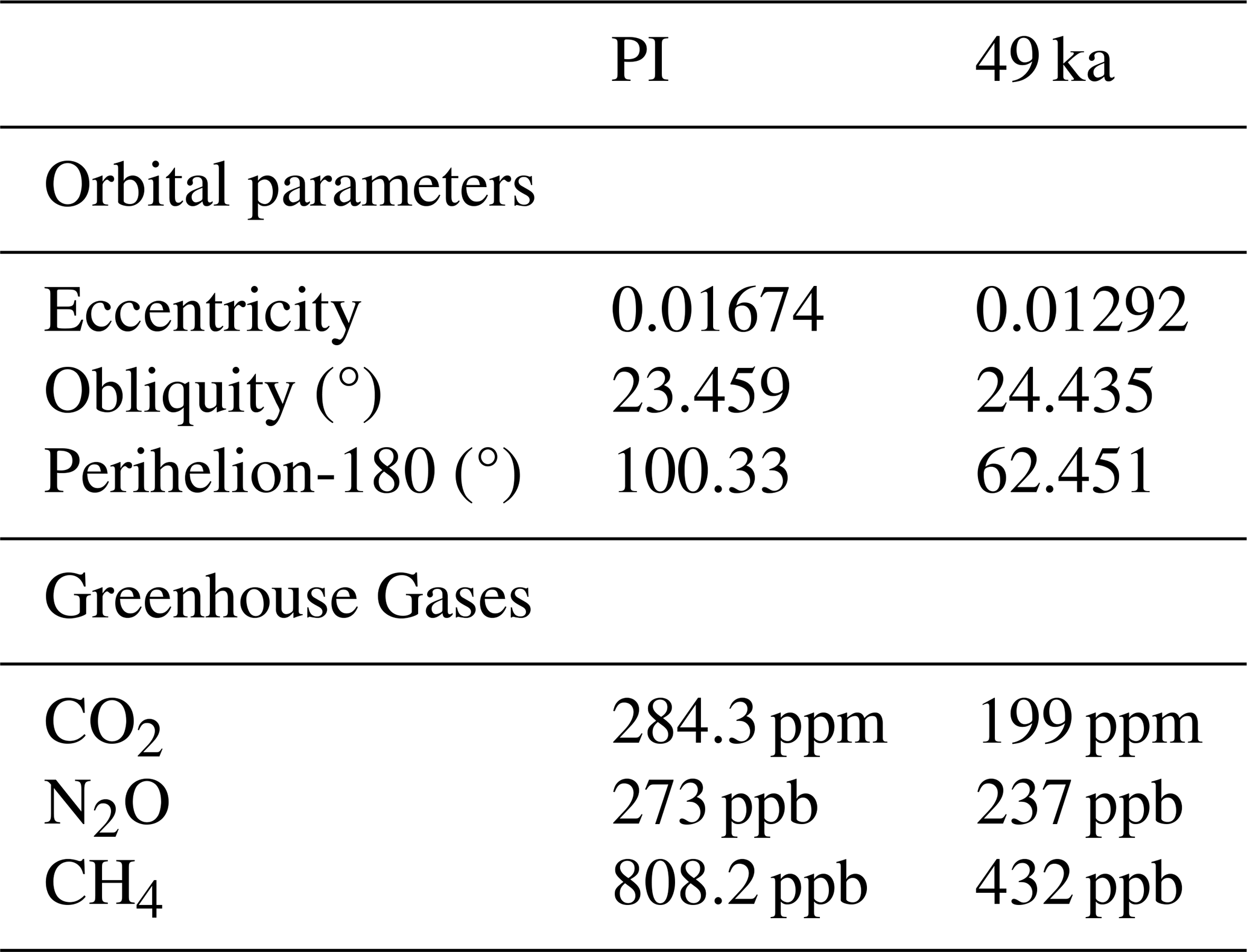
To investigate the climate around 49 ka, the boundary conditions are changed in a step-wise manner using the ACCESS-ESM1.5 model. The first experiment, 49ka-co, simulates a baseline climate with orbital parameters (Berger, 1978) and GHG concentrations (Köhler et al., 2017) being set to 49 ka values (Table 1). 49ka-co is run for 618 years (Fig. A1, cyan line).

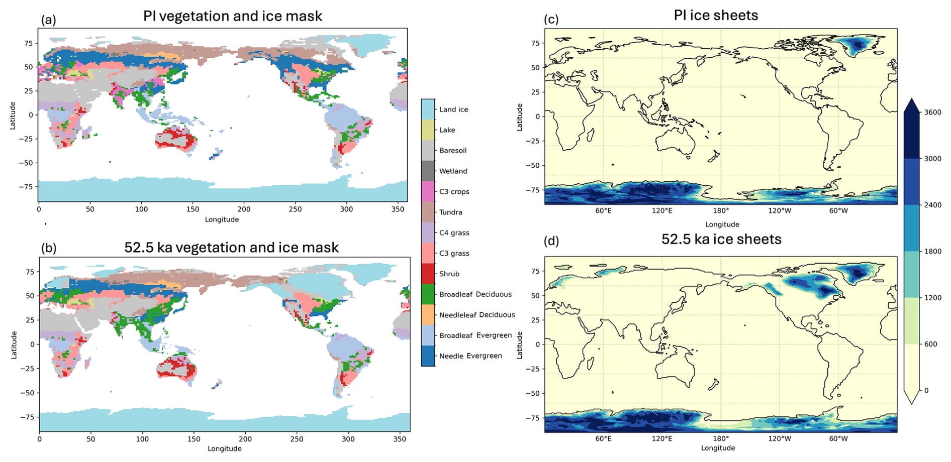
Figure 1 (a, b) Vegetation and ice mask changes at 49 ka compared to PI. The color indicates the dominant Plant Functional Type (PFT) of each grid cell. (c, d) Ice sheet thickness (m) and extent from Gowan et al. (2021) for PI and 52.5 ka (refer to the description in the text for the choice of 52.5 ka ice sheets).

The model uses prescribed Plant Functional Types (PFTs) that remain fixed during each individual simulation. We modified the PFT distributions in selected simulations to reflect the altered boundary conditions. Therefore, in a second step, 49ka-alb, we modify the land surface properties by incorporating only the ice-sheet extent (no topography yet) from Gowan et al. (2021) corresponding to 52.5 ka. We adopted the maximal scenario with an ice-capped Hudson Bay (Fig. 1d). This time period was chosen because the simulated ice sheet at 52.5 ka most closely matches the sea-level estimates for 48–52 ka, based on global seawater δ¹⁸O stack records (Shakun et al., 2015). The NH ice sheets at this time period include two separate ice sheets over the North American continent – Laurentide in the east and Cordilleran in the west – as well as the Greenland Ice Sheet and Fennoscandian and Eurasian ice sheets (Fig. 1d). Their extent and height are smaller than during the LGM (not shown), which featured a single, extensive LIS over North America and continuous ice sheet coverage from Eurasia to Scandinavia, fully covering the Barents Sea. The Antarctic Ice Sheet (AIS) at 52.5 ka also has a smaller extent compared to that of the LGM, especially over the Ross and Weddell Seas. At 52.5 ka, the LIS was up to 3 km thick, while the AIS was up to 3.6 km thick. In the present day, permanent ice cover in the NH is restricted to Greenland (Fig. 1c).

Table 2 Boundary conditions used in the different 49 ka experiments. Model years indicate the total number of years that the corresponding experiment has run for as shown in the time series of Fig. A1.

In the 49ka-alb experiment, additional modifications are introduced at different stages (Fig. A1, orange line). The vegetation cover is modified to reflect ice coverage by removing vegetation in ice-covered regions and converting needle leaf evergreen forests in areas between the Cordilleran and LIS to bare soil (Fig. 1a, b). These modifications align with the vegetation reconstruction from Allen et al. (2020) for 52 ka. Additionally, C₃ crops are removed, and replaced by the next two most dominant vegetation types in the corresponding grid cell. For example, in India, C₃ crop values are replaced by the broadleaf deciduous type and C₄ grass. In Europe and eastern North America, they are replaced by the broadleaf deciduous type and C₃ grass, while they are replaced by the broadleaf deciduous type in China. 49ka-alb (Fig. A1, orange line) starts from year 297 of 49ka-co, and was run for a total of 272 years with the above mentioned albedo and vegetation changes (Table 2). As can be seen in Fig. A1, 49ka-alb is not in complete equilibrium. To this 49ka-alb experiment, we add a gradual increase in surface salinity from year 547 (Fig. A1, magenta line), to account for the 44 m sea level drop relative to PI, based on the prescribed ice sheet, achieving a global average increase of +0.33 psu from PI levels. At year 729, the Bering Strait is closed.

Our final experiment, referred to as 49ka-full (Fig. A1, blue line, Table 2), starts at year 824, when the topography is adjusted to reflect conditions at 52.5 ka, based on Gowan et al. (2021), including an increase in ice sheet height and changes to the land-sea mask, such as the closure of the Bering Strait (done in the previous step), Hudson Bay, the Sahul and Sunda shelves, and the Tasman Gateway (Fig. 1). Nearest-neighbour interpolation is applied to determine vegetation types on newly exposed land. The river runoff is also adjusted at year 1258, to reflect the 52.5 ka topography. In total, 49ka-full is run for 760 years, with 325 years incorporating all the boundary conditions. In the Results section, we compare the averages of the last 100 years of 49ka-co, the last 50 years of 49ka-alb, and the last 100 years of the 49ka-full experiment (Table 2, Fig. A1, darker colors). Although the deep ocean has not fully equilibrated in the 49ka-co and 49ka-alb simulations, our comparison with the 49ka-full simulation focuses primarily on atmospheric circulation responses, which adjust to changes in boundary conditions much more rapidly than the ocean. Surface and atmospheric variables exhibit no systematic drift over the analysis period, supporting the robustness of the diagnostics presented here.

The ITCZ position is determined using the precipitation centroid index (Braconnot et al., 2007), which identifies the latitude that evenly divides the tropical precipitation amount between 20° S and 20° N. This approach effectively represents the center of mass of tropical rainfall distribution. The strength of the northern Hadley cell is determined by the maximum value of the atmospheric mass streamfunction, ψ, within the 400–600 hPa pressure range, while the strength of the southern Hadley cell is determined by its minimum value over the same vertical pressure range (Eq. 1).

$$\begin{array}{}\text{(1)}& \mathit{\psi }={\displaystyle \frac{\mathrm{2}\mathit{\pi }R\cos \mathit{\varphi }}{g}}\underset{\mathrm{0}}{\overset{p}{\int }}v\mathrm{d}p\end{array}$$

where, R is the radius of the earth, ϕ is latitude, g is gravitational acceleration, v is the meridional wind and p is pressure. ψ is expressed in Sverdrups (Sv), where 1 Sv = 10⁹ kg s⁻¹.

3 Results

3.1 Simulated glacial climate at 49 ka compared to PI

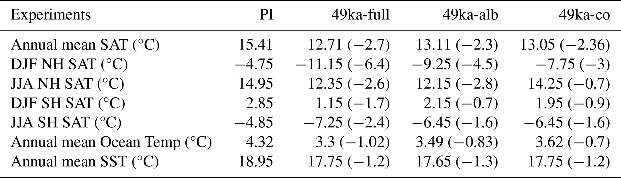
We first describe the 49ka-full experiment in comparison to PI. At 49 ka, the higher obliquity (24.43°) compared to PI (23.45°) results in slightly increased summer insolation in both hemispheres (Fig. A2). Despite the higher obliquity, the glacial simulation (49ka-full) exhibits substantial oceanic and atmospheric cooling due to lower GHG concentrations and extensive ice sheet expansion at this time (Fig. 2). Global annual mean surface air temperatures (SATs) at 49 ka are 2.7 °C lower than PI (Table A1 and Fig. 2a), with the NH cooling by 4.9 °C and the SH by 2 °C (not listed). The most pronounced cooling is simulated in ice sheet regions and northern high latitudes. Seasonal variations are evident in the NH (Table A1), where temperatures drop by 6.4 °C in winter (DJF) and 2.6 °C in summer (JJA). Over SH, DJF (austral summer) SATs are 1.7 °C lower, while JJA (austral winter) SATs are 2.4 °C lower (Table A1).

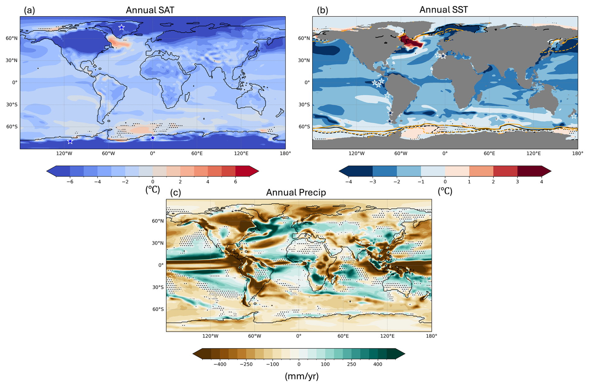
Figure 2 Annual mean anomalies of surface air temperature (SAT), sea surface temperature (SST), and precipitation for 49 ka climate (exp 49ka-full) compared to PI. Contours show seasonal mean 15 % sea ice concentration for (orange) 49 ka and (black) PI during DJF (dashed) and JJA (solid). Stippling indicates non-significant changes based on a Student's t-test at the 95 % confidence level. Stars in panels (a) and (b) indicate qualitative estimates of the changes between Greenland Interstadial (GI 13) and PI climate, as inferred from the proxy records (MDO1-2444, ODP-977A,MD95-2043, MD01-2443,MD95-2042 (Martrat et al., 2007); ODP-1233 (Kaiser et al., 2005); TR163-19 (Lea et al., 2000); RC13-110 (Feldberg and Mix, 2003); ODP846B (Martínez et al., 2003); TG-7 (Calvo et al., 2001); MD97-2120 (Pahnke et al., 2003); MD07-3128 (Caniupán et al., 2011); EPICA Dronning Maud Land (EPICA community members, 2006); WAIS (WAIS Divide Project Members, 2015); NGRIP (Huber et al., 2006; Kindler et al., 2014); SO188-17286-1 (Lauterbach et al., 2020)). Dark (light) blue stars represent much colder (slightly colder) climate in proxy records.

Global mean ocean temperature is 1 °C lower, and global annual mean sea surface temperature (SST) (Fig. 2b) is reduced by 1.2 °C (Table A1). The simulated SATs and SSTs anomalies show a good agreement with proxy records indicating a qualitative estimate of the changes between Greenland Interstadial (GI 13; 49ka-50ka) and PI climate (Fig. 2a,b). Higher SSTs in the Labrador region are associated with a stronger AMOC in 49ka-full, with a transport rate of 31 Sv (about 10 Sv greater than the PI value). This strengthening is attributed to topographical changes and the presence of ice sheets, which enhance westerly winds over Baffin Bay and weaken them over the Labrador Sea (Fig. A3, middle panels). These wind changes modify the North Atlantic gyres, leading to an overall strengthening while shifting the separation between the subpolar and polar gyres southward and orienting the subpolar gyre in a more zonal direction (Fig. A3, bottom panels). A strengthening of the cyclonic circulation in the Labrador Sea is also simulated, which increases the westward transport of warm water from south of Iceland to the Labrador Sea and further strengthens the AMOC (reflected by the increase in mixed layer depth in this region in 49ka-full compared to PI, Fig. A3, top panels). The stronger AMOC also influences sea ice extent. During boreal winter, the sea ice edge at 49 ka expands in the North Pacific and Nordic Sea sectors but retreats in the Labrador Sea due to the influx of warm water (Fig. 2b, orange dashed line compared to black dashed line). In boreal summer, the 49 ka sea ice edge is similar to PI across most regions, except in the Nordic seas, where the sea ice edge extends further south than in PI by 5 to 6° latitude (Fig. 2b, orange solid line compared to black solid line). In the SH, austral summer sea ice retreats in the South Atlantic as stronger North Atlantic Deep Water (NADW) formation leads to a deep-ocean warming of about 0.3 °C (not shown), and this warm water gets upwelled in the South Atlantic (Fig. 2b, orange dashed line compared to black dashed line). However, the austral winter sea ice edge remains similar to PI in the South Atlantic while expanding in the Indian and Pacific sectors of the Southern Ocean (Fig. 2b, orange solid line compared to black solid line).

Drier conditions are simulated at 49 ka compared to PI over NH high-latitude land regions, particularly over the LIS, due to colder conditions and reduced atmospheric moisture availability (Fig. 2c). However, precipitation increases in the North Atlantic and Eurasia between 30° N and 60° N, as well as over India and East Asia. In contrast, most land areas in the SH display decreased precipitation, except over northern Australia, parts of Southeast Africa, and over eastern Brazil.

3.2 Impact of 49 ka boundary conditions on the circulation over North Atlantic and Eurasia

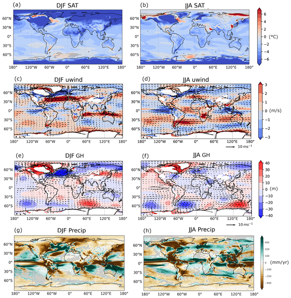
At 49 ka (experiment 49ka-full), the presence of large ice sheets over North America significantly alters the atmospheric circulation, particularly in the North Atlantic region. In DJF, the westerlies over the North Atlantic strengthen due to the strong meridional temperature gradient and shift by ∼ 6° southward compared to PI (Figs. 3a, c, and 4a), with a more zonal flow replacing the northeast-southwest tilt of the wind field (Fig. 5). This pattern is evident both at the surface and at the jet stream level in the upper troposphere (Fig. A4). Geopotential height (GH) differences (Fig. 3e) indicate that the LIS induces a high-pressure system (not shown) over North America, initiating a Rossby wave response. This Rossby wave causes a southward shift of the Icelandic low and a weakening of the Azores High, contributing to the zonal orientation of the westerlies (Figs. 3c, 5, and A5). The southward shift and more zonal orientation of the jet alter moisture-bearing storm tracks, which in PI were tilted southwest-northeast, to a more southerly pathway at 49 ka. This reorganization of pressure systems (not shown), with a negative GH anomaly extending from the North Atlantic to eastern Eurasia (Fig. 3e), alters precipitation patterns, enhancing precipitation over the North Atlantic and western Europe (Fig. 3g). However, colder conditions over Eurasian landmasses lead to drier conditions inland in DJF, despite negative GH anomalies (Fig. 3a, e, g).

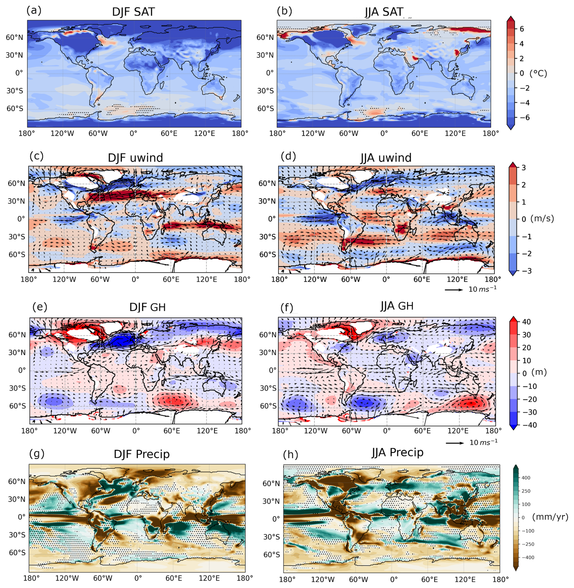
Figure 3 Anomalies between 49ka-full and PI for (a, b) SAT (°C), (c, d) zonal winds at 850 hPa (m s⁻¹) overlaid with 850 hPa wind vector anomalies (m s⁻¹), (e, f) geopotential height at 850 hPa (m) with zonal mean removed and overlaid with 850 hPa wind vector anomalies (m s⁻¹), and (g, h) precipitation (mm yr⁻¹) during (left) DJF and (right) JJA. Stippling in panels (a), (b) and (g), (h) indicates non-significant changes based on a Student's t-test at the 95 % confidence level. The white space in panels (c)–(f) indicates the ice mask at the 850 hPa level.

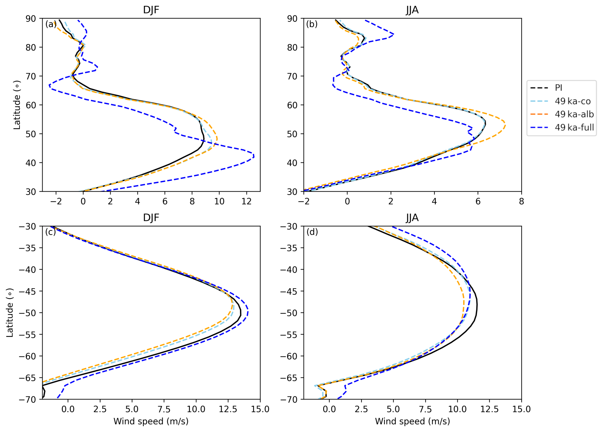
Figure 4 Zonal winds at the 850 hPa level (m s⁻¹) averaged (top) over the North Atlantic (80° W : 0° E) and (bottom) averaged over all longitudes representing westerlies over the SH during (a, c) DJF and (b, d) JJA seasons.

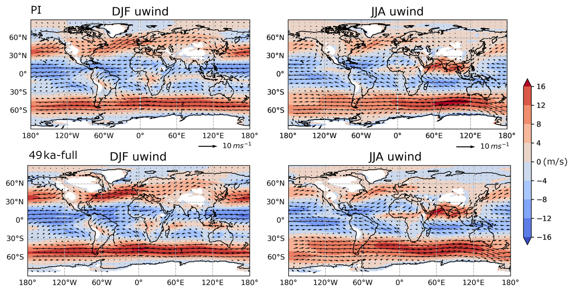
Figure 5 Zonal winds at 850 hPa (m s⁻¹) overlaid with 850 hPa wind vectors (m s⁻¹) in (left) DJF and (right) JJA for (top) PI and (bottom) 49ka-full. The white space the ice mask at the 850 hPa level.

The westerlies are also shifted southward in JJA (Figs. 3d and 4b), with the flow remaining more zonal in 49 ka than during PI (Fig. 5, right panels), coinciding with a positive GH anomaly over the Labrador Sea region while a negative GH anomaly forms over Europe (Fig. 3f). These GH anomalies enhance the westerly flow and contribute to moisture transport convergence (not shown) toward the Eurasian landmass, increasing precipitation along the westerlies in the North Atlantic Ocean and over parts of Eurasia (Fig. 3d, f, h). In addition, minor cooling over Eurasia (Fig. 3b) further contributes to the increased precipitation. Precipitation also increases north of 60° N in Asia (Fig. 3h) due to higher specific humidity (not shown) resulting from warmer conditions and the development of a negative GH anomaly (Fig. 3b, f). The warming in this region arises from the topographical changes corresponding to 49 ka, where ocean points have been converted to land. Since land has a lower heat capacity than the ocean, it warms more rapidly in summer, amplifying the temperature-driven moisture increase. Conversely, north of 60° N in Europe precipitation decreases. This is due to the colder north-easterly winds and the presence of a blocking high over the Labrador-Greenland sector, which suppresses rainfall in these areas.

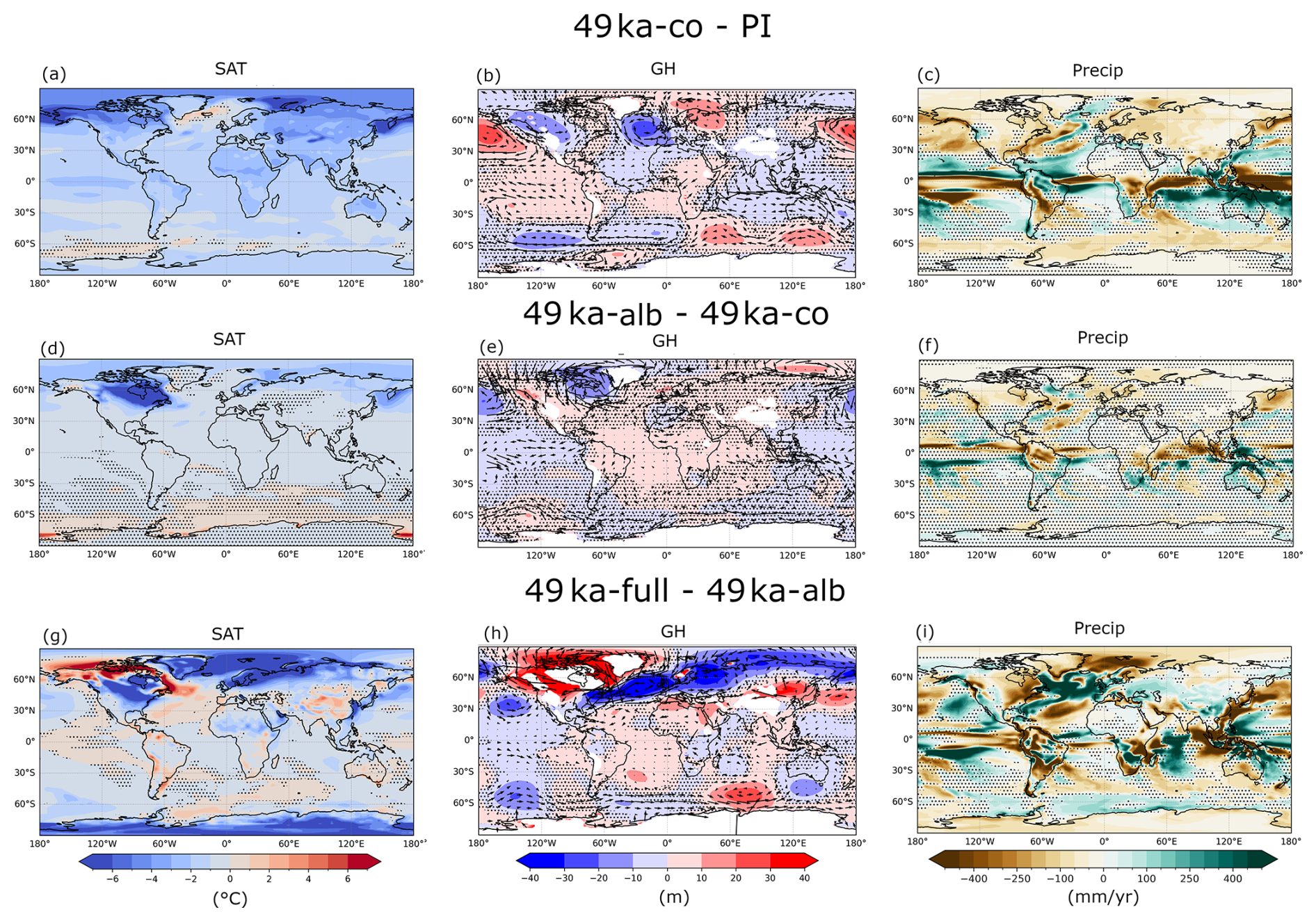
Figure 6 DJF (a, d, g) SAT (°C), (b, e, h) geopotential height (m) overlaid with wind vector anomalies at 850 hPa and precipitation (mm yr⁻¹) anomalies for (a–c) 49ka-co minus PI, (d–f) 49ka-alb minus 49ka-co, (g–i) and 49ka-full minus 49ka-alb. Stippling indicates non-significant changes based on a Student's t-test at the 95 % confidence level. The white space in panels (b), (e), and (h) indicates the ice mask at the 850 hPa level.

The role of individual boundary conditions becomes evident in the 49ka-co experiment, which includes only orbital parameters and GHGs. During DJF, strong cooling in the 49ka-co experiment reduces moisture availability, leading to widespread drying over NH landmasses (Fig. 6a, c). The westerlies are enhanced and slightly shift southward (∼ 1°) (Figs. 4a and 9a). This shift is accompanied by a low-pressure anomaly over the North Atlantic and a high-pressure system over Europe, which enhances subsidence and suppresses precipitation over Europe (Fig. 6b, c). This pattern is consistent with the overall drying trend in the NH, except for a small increase in precipitation over the North Atlantic Ocean (Fig. 6c), likely due to storm activity in this region. In 49ka-alb, changing the vegetation and albedo has little impact compared to 49ka-co, except over northern North America (Fig. 6d, f), where cooling is enhanced by 8 °C and drying increases by 25 % due to the albedo change over the LIS. The westerlies intensify further compared to 49ka-co, but their position shifts back to the PI configuration (Fig. 4a). The GH response features a low-pressure anomaly over the Hudson Bay and Labrador Sea, which is consistent with some increased precipitation in this region (Fig. 6e, f).

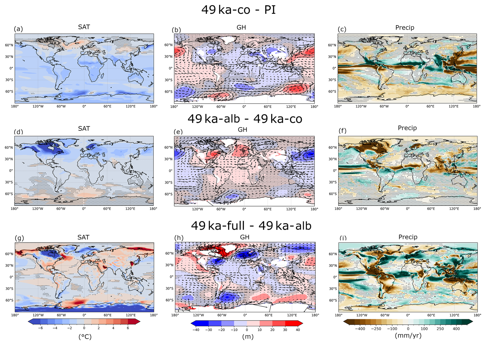
Figure 7 Same as Fig. 6 but for JJA.

In JJA, the 49ka-co experiment shows no change in westerly strength and position over the North Atlantic (Figs. 4b, 7b, and 9b) and modest temperature and little significant precipitation changes over the NH landmass (Fig. 7a, c). In contrast, the 49ka-alb experiment exhibits pronounced drying over the Laurentide region and northern Europe, driven by intense cooling from albedo changes and persistent high pressure over these regions (Fig. 7d–f). While the westerlies strengthen in 49ka-alb, their position remains unchanged (Figs. 4b and 9b). This intensification leads to slightly wetter conditions inland over Eurasia in the 49ka-alb scenario.

In summary, only the full implementation of the ice sheet, including its topography, can induce a significant planetary wave response in the atmosphere, with southward-shifted and intensified North Atlantic westerlies (Figs. 4a, 6, 7, and 9). This response results in substantial drying over the northern high-latitude landmasses, including the Laurentide region during DJF, along with increased milder and wetter conditions over Eurasia during JJA.

3.3 Impact of 49 ka boundary conditions on tropical and SH atmospheric circulation.

In DJF, the presence of the LIS forces a southward shift of the Ferrell cell. This displacement further leads to a southward migration of the NH Hadley cell's southern edge, shifting from 7.5° S in PI to 11° S in 49ka-full (Fig. 8a, see zero contour), and results in a globally averaged ITCZ shift of approximately 1.5° southward in DJF (Figs. 3g and 9a). Additionally, the NH Hadley cell strengthens by 20 Sv relative to PI (refer to Sect. 2.2 for diagnostics). The southward shift of the NH Hadley cell and ITCZ during DJF is also captured in 49ka-co (Fig. 8c), where the NH Hadley cell strengthens by +11 Sv relative to PI. The shift in the ITCZ is driven by peak summer insolation in the SH due to higher obliquity at 49 ka. However, the magnitude of change in 49ka-co is smaller than in 49ka-full (Figs. 8a and 9a), with an ITCZ shift of 0.6°. Implementing albedo changes in 49ka-alb enhances the Laurentide cooling, further strengthening the NH Hadley cell (by +8 Sv), albeit without additional displacement (9.5° S in 49ka-co vs. 9.6° S in 49ka-alb) (Fig. 8c, e). The minor shift in the NH Hadley cell and ITCZ position explains why lower latitude precipitation changes remain insignificant between 49ka-alb and 49ka-co (Fig. 6c, f). However, the inclusion of topography in 49ka-full results in a slight additional strengthening of the NH Hadley cell and a more substantial southward ITCZ shift (by 1.5° relative to 49ka-alb), due to the stronger temperature gradient between the two hemispheres (Fig. 9a, Table A1).

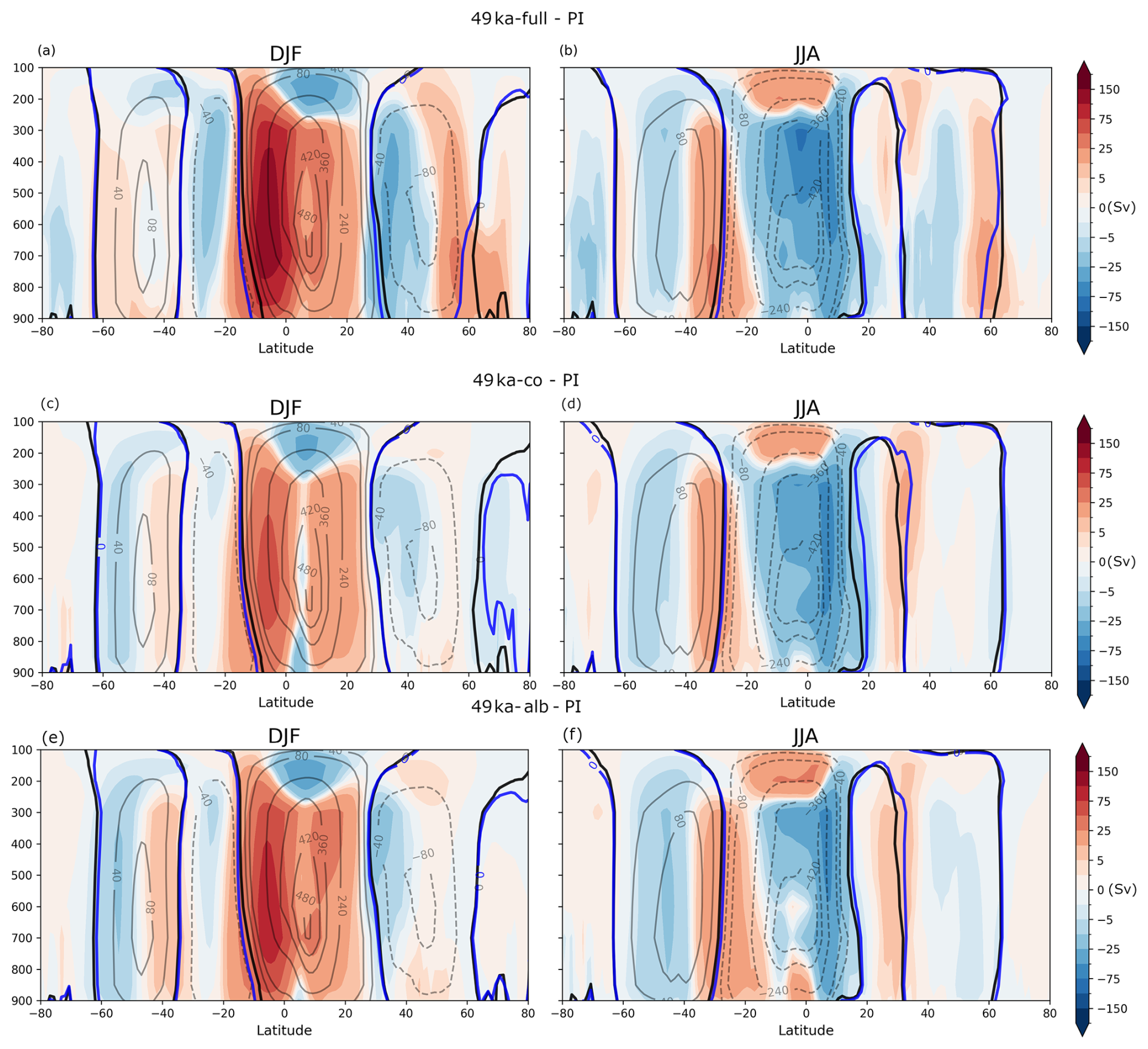
Figure 8 Atmospheric mass streamfunction (Sv) anomalies (shading) between (a, b) 49ka-full and PI, (c, d) 49ka-co and PI, and (e, f) 49ka-alb and PI, for (left) DJF and (right) JJA. Contours (solid = positive; dashed = negative) are PI (black) absolute streamfunction values. The thick black and blue lines represent the zero contour for PI and 49 ka experiments, respectively.

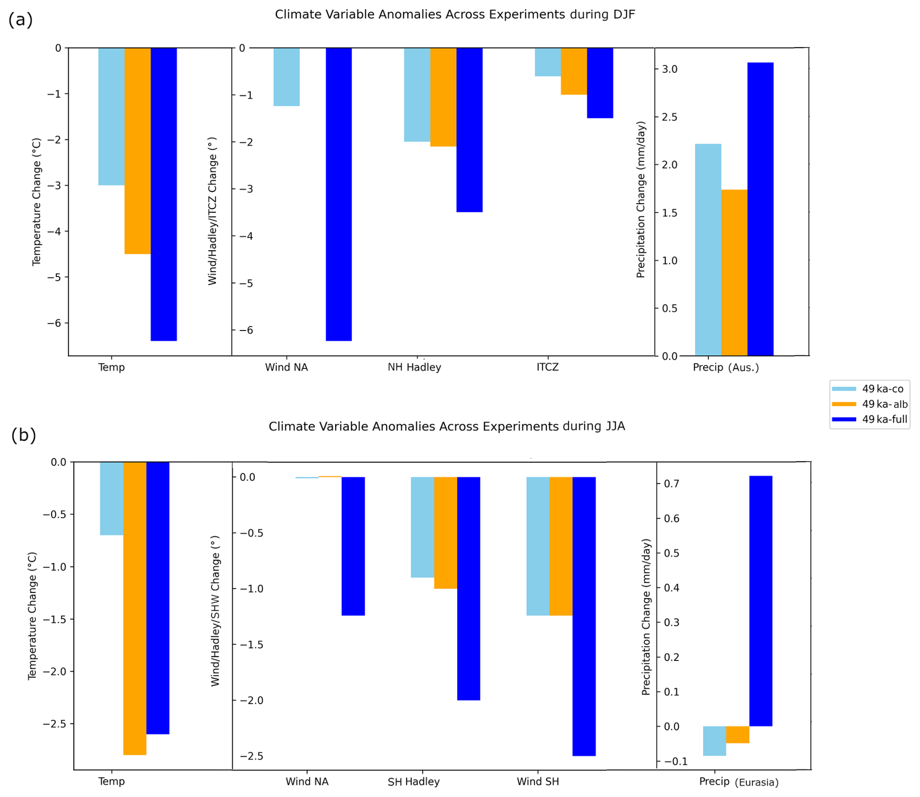
Figure 9 Summary of key atmospheric responses across experiments. (a) DJF anomalies: NH SAT (°C) (left); latitudinal shifts (°) (middle) in westerlies (calculated as the latitude of the maximum wind speed averaged over the North Atlantic (80° W–0° E, 30° N–90° N)), NH Hadley cell's southern edge, and globally averaged ITCZ position; and northern Australian precipitation (116° E–152° E, 25° S–12° S, mm d⁻¹) (right). (b) JJA anomalies: NH SAT (°C) (left); latitudinal shifts (°) (middle) in westerlies averaged over the North Atlantic, SH Hadley cell's southern edge (°), westerlies averaged over the SH; and precipitation changes over Eurasia (60° W–80° E, 48° N–60° N) (right). Results are shown for the 49ka-co (cyan), 49ka-alb (orange), and 49ka-full (blue) experiments, with all values presented as anomalies relative to PI. Negative values in latitudinal shifts indicate an equatorward shift.

During JJA, the southern edge of the SH Hadley cell shifts northward by 2° in 49ka-full, moving from 32° S in PI to 30° S, along with a northward shift of the Southern Ferrel cell (Fig. 8b, see zero contour). This shift causes a slight northward migration of the global ITCZ (Fig. 3h), while the SH Hadley cell strengthens by 35 Sv. In 49ka-co, a slight warming over the North Atlantic and stronger cooling in the SH shifts the SH Hadley cell's southern edge to 31° S, accompanied by a strengthening of +22 Sv (Figs. 8d and 9b). The changes in 49ka-alb do not alter the SH Hadley cell's latitudinal position significantly but weaken its strength to PI levels (Figs. 8f and 9b), due to intensified Laurentide cooling. As a result, precipitation changes in the lower latitudes remain small (Fig. 7c, f). Temperature contrasts between hemispheres are reduced by ice sheet topography (Table A1, comparison of JJA NH minus SH SAT differences between 49ka-full, 49ka-alb and 49ka-co), which induces localized warming in Siberia and strong Antarctic cooling, and by changes in the land-sea mask with the replacement of ocean grid cells by land. This reduced thermal gradient with warming in the NH leads to a slight northward ITCZ shift, further strengthening the SH Hadley cell and shifting it an additional 1° northward, toward the warmer hemisphere, relative to 49ka-alb.

The SH westerlies also exhibit distinct responses across the simulations. In DJF, they weaken slightly in 49ka-co and 49ka-alb, accompanied by a small northward shift (Fig. 4c). In contrast, in 49ka-full, they remain in the same position as in PI but strengthen due to the increased height and extent of the AIS. During JJA, the SH westerlies weaken across all 49 ka simulations compared to PI, with the most pronounced weakening occurring in the experiment where albedo is changed (Fig. 4d). However, in 49ka-full, they shift northward by 2.5°, a displacement linked to the northward shift of the SH Hadley cell in 49ka-full (Figs. 4d and 9b).

3.4 Impact of 49 ka boundary conditions on Australian rainfall

The implementation of 49 ka boundary conditions leads to a notable increase in Australian rainfall during the monsoon season (Figs. 3g and 9a). This section focuses on the large-scale processes driving this regional rainfall response. While a detailed analysis of monsoon changes in other regions lies beyond the scope of this study, our results underscore the influence of NH ice sheets on hemispheric-scale atmospheric dynamics.

The presence of NH and larger AISs induces substantial atmospheric circulation changes by modifying the Hadley and Ferrel cells and influencing the westerlies in both hemispheres. These shifts propagate through the atmosphere, altering surface pressure systems and triggering a hemispheric-scale response.

During DJF, the full boundary conditions in 49ka-full force a southward shift of the Hadley and Ferrel cells (Fig. 8a), enhancing subsidence over East Asia around 40° N and leading to drier conditions (Fig. 3e, g). This southward displacement of the NH Hadley cell extends across hemispheres, impacting Australian rainfall by shifting convergence southwards along with the ITCZ (Fig. 8a). These changes explain the wetter conditions in northern Australia and drier conditions over the Maritime Continent (Fig. 3g). A comparable but weaker response is simulated in the 49ka-co experiment (Fig. 6c). In contrast, changes in albedo do not impact Australian precipitation significantly (Fig. 6f). However, modifying the topography induces wetter conditions in northern Australia driven by shifts in the Hadley cell and ITCZ, while southern Australia experiences drier conditions (Fig. 6h, i).

During JJA, in response to the 49 ka boundary conditions, most of Australia experiences drying (Fig. 3h), primarily due to the establishment of blocking high-pressure systems south of the continent (Fig. 3f). These high-pressure systems reinforce subsidence and restrict moisture transport from the Southern Ocean into the Australian region (not shown). However, the drying response is not significant over central Australia and remains less pronounced along the eastern and western edges of the continent. The southwestern part of Australia becomes wetter, while the southeastern region experiences drying, due to the northward displacement of the westerlies, resembling a negative winter Southern Annular Mode (SAM). Significant drying also occurs across northern Australia and much of the Maritime Continent south of the equator.

When only orbital parameters and GHGs are modified, the SH Hadley cell shifts northward and strengthens. However, in this scenario, the weakening of the SH westerlies and the southward displacement of subtropical high-pressure systems result in increased rainfall over southern Australia (Fig. 7b, c). Introducing albedo changes alone has little impact on the Australian climate (Fig. 7d–f). However, when ice sheet topography is incorporated, the northward shift in SH westerlies linked with the strengthening and equatorward displacement of the SH Hadley cell causes enhanced subsidence and thus drier conditions over Australia, coinciding with the northward ITCZ migration (Figs. 7i and 4d). Compared to the PI climate, this drying effect is somewhat mitigated, as the westerlies – despite their northward shift – remain weaker overall.

4 Discussion

Our simulations of the 49 ka glacial climate reveal a complex interplay of ice sheet topography, GHG forcing, and orbital configurations. The results underscore how large-scale climatic features, such as atmospheric circulation patterns, precipitation distribution, and ocean circulation, respond to glacial boundary conditions. Additionally, much of the existing research has focused primarily on the North Atlantic region, driven by the greater availability of paleoclimate data from this area and the presence of extensive North American ice sheets that strongly influenced both regional and global climate. Our results add to this literature by demonstrating that the influence of glacial ice sheets extends well beyond the North Atlantic, with significant climatic impacts also occurring in other regions, including the SH. Although the present experimental design does not fully isolate the individual contributions of the Laurentide and AISs, sensitivity experiments and previous studies indicate that the NH ice sheet topography, dominated by the LIS, provides the primary control on midlatitude circulation changes. SH circulation changes arise from the combined influence of both ice sheets, with Antarctic topography acting primarily through modulation of interhemispheric temperature gradients.

Here, the simulated state in the 49ka-full experiment represents an interstadial climate. The global annual mean cooling in 49ka-full relative to PI (a 2.7 °C reduction in global SATs) aligns with the expected glacial forcing associated with lower GHG concentrations and extensive ice sheet expansion. The pronounced winter cooling in the NH, exceeding 6 °C, is similar to PMIP4 simulations of LGM climate, with ice sheet-driven albedo changes amplifying high-latitude cooling during glacial periods (Kageyama et al., 2021). This magnitude of cooling from PI is also broadly consistent with other MIS 3 modelling studies, though direct comparisons are not possible as applied boundary conditions between other MIS 3 studies and ours were different. For example, Guo et al. (2019) found a 2.9 °C globally averaged annual mean cooling over a 38 ka time slice using the Norwegian Earth System Model (NorESM). Simulations using the Community Climate System Model version 3 (CCSM3) model suggest stronger cooling, with Merkel et al. (2010) reporting a 3.4 °C drop at 35 ka, and Zhang et al. (2014b) estimating 3.5 °C at 38 ka.

4.1 Changes in AMOC

Proxy records suggest significant AMOC variability during the MIS 3 period, with stronger AMOC during the onset of interstadials (Böhm et al., 2015; Henry et al., 2016; Menviel et al., 2020), and weak AMOC during stadials. The processes driving this AMOC variability are still debated (Menviel et al., 2020). Model simulations of MIS 3 climates show a range of AMOC responses depending on the prescribed boundary conditions, particularly the configuration of Northern Hemisphere ice sheets. For example, CCSM3 simulations at 35 and 44 ka show AMOC reductions of approximately 40 % (Merkel et al., 2010) and 50 % (Brandefelt et al., 2011), respectively, while a University of Victoria (UVic)-ESM simulation at ∼ 40 ka produces a ∼ 33 % reduction relative to PI (Saini et al., 2024). In contrast, other simulations show little change or a modest strengthening of the AMOC. For example, Zhang et al. (2014b) simulated a ∼ 7 % strengthening at 38 ka using CCSM3, while Guo et al. (2019) reported a ∼ 13 % strengthening at 38 ka using NorESM. Similarly, Van Meerbeeck et al. (2009) simulated a 22 % increase in AMOC strength during MIS 3 compared to PI (estimated from Menviel et al., 2008) using the LOVECLIM model.

The simulated AMOC in our 49ka-full simulation is strong (31 Sv) with a 47 % increase relative to PI. This strengthening is driven by changes in the LIS, which enhances westerly winds over Baffin Bay while weakening them over the Labrador Sea, intensifying the cyclonic circulation in the Labrador Sea and facilitating the transport of warm, saline waters to the region. This process is also associated with sea ice retreat in polar regions, which further reinforces AMOC strength. These findings align with earlier modelling studies emphasizing the role of topography and ocean–atmosphere interactions in AMOC enhancement (Pausata et al., 2011; Zhang et al., 2014a; Hu et al., 2015; Brown and Galbraith, 2016; Klockmann et al., 2018; Sherriff-Tadano et al., 2018; Guo et al., 2019). For example, Pausata et al. (2011) demonstrated that the presence of an extensive ice sheet during the LGM enhanced AMOC by altering atmospheric circulation patterns. However, their simulations also showed that the cooling effects from lower GHG concentrations and increased albedo suppressed AMOC strength. In our 49ka-full experiment, these cooling effects appear to be offset by the relatively high insolation state at 49 ka, allowing topographical impacts to dominate.

The simulated AMOC in 49ka-full is stronger than that reported in most previous MIS 3 simulations. However, the spread among MIS 3 simulations highlights the sensitivity of AMOC strength to the prescribed LIS configuration. Previous studies focusing on LGM climate have shown that changes in North Atlantic westerlies induced by the presence of the LIS can strengthen the AMOC through enhanced wind-driven circulation and deep-water formation (Muglia and Schmittner, 2015). Consistent with this mechanism, the stronger AMOC in our 49ka-full simulation is associated with LIS-driven changes in atmospheric circulation and enhanced westerlies over the North Atlantic. Conversely, changes in LIS height have also been shown to strongly affect AMOC stability and can trigger transitions between different overturning states (Zhang et al., 2014a), indicating that different ice-sheet reconstructions can produce markedly different AMOC responses. Since the LIS evolved substantially throughout MIS 3 and remains poorly constrained (Malmierca-Vallet and Sime, 2023), alternative but equally plausible ice-sheet configurations may yield weaker AMOC states than simulated here. This sensitivity is consistent with evidence for large AMOC variability during MIS 3, including rapid transitions and possible overshoots following Heinrich stadials. We therefore interpret the strong AMOC in 49ka-full as a response to the specific ice-sheet configuration prescribed in our experiments rather than as a robust feature of all MIS 3 climates.

Evidence based on foraminifer assemblages and mineral grains in ice-rafted debris also suggests a northward retreat of sea ice and higher temperatures in the Labrador Sea between ∼ 56 and 49 ka, potentially driven by the insolation maxima (Griem et al., 2019). After 49 ka, sea ice variability increased, with near-perennial sea ice cover during most stadials and seasonal ice-free conditions during interstadials. However, it remains uncertain whether interstadials reflect a mean state or are primarily linked to Dansgaard–Oeschger (D-O) variability.

4.2 Changes in NH westerlies

The simulated changes in the North Atlantic westerlies and associated precipitation patterns during DJF highlight the critical role of ice sheet topography in driving atmospheric circulation (Fig. 9a). At 49 ka, the surface westerlies shift southward and adopt a more zonal flow (Fig. 3), aligning with previous studies (Löfverström et al., 2014; Ullman et al., 2014; Pausata et al., 2011; Kageyama et al., 2021; Stadelmaier et al., 2024), which emphasize the influence of glacial ice sheet topography on jet stream reorganization. Our results further expand on this, demonstrating that the high-pressure system induced by the LIS initiates a Rossby wave response, shifting the Icelandic low southward and weakening the Azores High. These circulation changes lead to reduced precipitation over NH landmasses during DJF.

During JJA, the changes in westerlies and pressure result in increased rainfall over Eurasia (Fig. 9b), with the jet stream extending further inland. Additionally, this rainfall increase is supported by milder land temperatures and enhanced moisture availability (not shown). Our findings on seasonal precipitation changes are consistent with those of Löfverström et al. (2014), as the ice sheet configuration used in our study closely resembles their MIS 4 ice sheet setup. However, while their study reports a fully zonal orientation of the jet stream only during the LGM, our results demonstrate that this change can also occur with a MIS 3 ice sheet configuration, suggesting a dynamic response to glacial ice sheets earlier in the glacial period.

4.3 Changes in tropical atmospheric circulation and SH westerlies

The presence of ice sheet topography leads to a more pronounced southward shift of the NH Hadley cell during DJF and a stronger northward shift of the SH Hadley cell during JJA, compared to our simulations that include only GHG concentrations, orbital parameters, and an ice mask at 49 ka (Fig. 9a, b). This enhanced Hadley cell shift in 49ka-full drives a more substantial southward displacement of the ITCZ during DJF (Fig. 9a). Consequently, the northern tropics experience drier conditions, while precipitation increases in the southern tropics, consistent with the mechanisms proposed by Chiang and Bitz (2005).

During JJA, LIS topography induces warming over Siberia, in agreement with previous studies (Liakka and Löfverström, 2018; Bakker et al., 2020), which attribute this warming to large-scale atmospheric circulation changes driven by pressure differences linked to LIS height. In contrast, AIS topography enhances cooling over Antarctica during austral winter. This interhemispheric contrast, i.e. relatively warmer conditions in the NH and colder conditions in the SH, pushes the ITCZ northward and strengthens the SH Hadley cell. Additionally, the SH Hadley cell northward shift is associated with the northward displacement of the SH westerlies (Fig. 9b), consistent with Ceppi et al. (2013), who demonstrated that interhemispheric teleconnections link ITCZ migration with changes in Hadley cell strength and SH jet positioning. Likewise, NH cooling during DJF drives a southward shift of the North Atlantic westerlies, influencing the Hadley cell strength and position, and pushing the ITCZ closer to the equator.

These circulation shifts generate regional impacts. Increased subsidence over East Asia creates a high-pressure anomaly, leading to drier conditions, while the southward-shifted ITCZ enhances convergence over Australia, increasing rainfall. The larger shift in the ITCZ and the NH Hadley cell coincides with the maximum increase in Australian rainfall (Fig. 9a).

The weakening of the SH westerlies during both DJF and JJA under a high-obliquity climate (49ka-co and 49ka-alb) compared to a low-obliquity climate (PI) aligns with findings from Timmermann et al. (2014). However, the increased height and extent of the AIS counteract this weakening during DJF, leading to SH westerly intensification in 49ka-full. Additionally, our results indicate that NH westerlies strengthen with albedo changes relative to orbital parameter and GHG adjustments, whereas SH westerlies weaken under the same conditions (Fig. 4). Introducing topographical changes induces an equatorward shift in both NH and SH westerlies during their respective winter seasons (Fig. 4a, d).

Overall, our study reveals nonlinear interactions between large-scale atmospheric circulation, surface westerlies, and precipitation patterns under different combinations of boundary conditions (Fig. 9). Orbital forcing, GHGs, albedo, and ice sheet topography collectively shape these interactions in a nonlinear manner.

4.4 MIS 3 hydroclimate in Australia

Proxy records from marine sediments, lake sediments, and river systems show that Australia experienced spatially variable climates during MIS 3, with greater-than-modern mean water availability peaking between ∼ 49 and ∼ 40 ka (Kemp et al., 2019). Wet conditions, especially in central and northern Australia between ∼ 50 and ∼ 45 ka, are linked to an intensified Australian monsoon driven by the summer insolation peak. Our model results align with these observations, showing increased annual precipitation over much of Australia at 49 ka, with particularly intensified monsoonal rainfall in the northern regions (Figs. 2c and 3g). The increase in monsoonal rainfall during austral summer is consistent with a southward displacement of the ITCZ due to the intensified NH Hadley cell, driven by increased SH insolation in response to high obliquity. However, our results also reveal that the southward shift of the ITCZ and Hadley cell occurs in the 49ka-full simulation (which includes ice sheet topography) as well as in the 49ka-co and 49ka-alb simulations (which lack ice sheet topography). Despite this, the intensified Australian monsoon rainfall is more pronounced in the 49ka-full experiment, as the presence of ice sheets induces larger shifts of the Hadley cell and ITCZ.

Our simulations generally show an insignificant response in southern Australian annual rainfall at 49 ka, although austral winter exhibits some drier conditions. These results are consistent with those of Weij et al. (2024), in which speleothem growth rates from southwest and southeast Australia indicate drier-than-modern conditions around 49 ka. In contrast, paleo records from Kemp et al. (2019) suggest increased rainfall in southern Australia. The wetter signal in that study is interpreted as a response to changes in the SH westerlies, involving either strengthening or an equatorward shift. While the wind response is consistent with the equatorward shift simulated in the 49ka-full experiment, the rainfall response is not reproduced, indicating that southern Australian precipitation is not solely controlled by latitudinal shifts of the westerlies in ACCESS-ESM1.5. Instead, rainfall anomalies appear to be more strongly influenced by persistent subtropical high-pressure anomalies and associated subsidence over the Australian continent, which suppress moisture transport convergence despite the shift in westerlies. This may indicate limitations in the simulated coupling between storm-track variability and regional precipitation under glacial boundary conditions. However, the contrasting interpretations from available proxy records also suggest that hydroclimate conditions in southern Australia during MIS 3 remain uncertain.

5 Conclusions

Our results, based on a stepwise set of MIS 3 boundary condition experiments, underscore the impacts of orbital forcing, greenhouse gases, surface albedo, and ice-sheet topography on global atmospheric circulation and regional hydroclimate. Orbital parameters and greenhouse gases alone produce limited dynamical shifts, while the addition of ice-sheet albedo primarily enhances high-latitude cooling without substantially altering circulation patterns. In contrast, the presence of NH ice sheets during MIS 3 strengthens and shifts the North Atlantic westerlies equatorward by 6° in DJF and 4° in JJA, leading to increased precipitation over the North Atlantic in both seasons, while over the Eurasian landmass precipitation increases in boreal summer but decreases in winter due to colder conditions. These ice sheet-induced changes affect the global atmospheric circulation, with a southward shift of the NH Hadley cell and ITCZ during DJF, resulting in enhanced monsoonal rainfall over northern Australia, while producing a comparatively weak hydroclimatic response in southern Australia. Regional differences, particularly between northern and southern Australia, reflect contrasting dynamical controls, with northern Australia dominated by monsoon and ITCZ-related moisture convergence, and southern Australia more strongly influenced by subtropical high-pressure anomalies and associated subsidence. These patterns are broadly consistent with proxy evidence indicating spatially heterogeneous hydroclimate conditions during MIS 3, with records suggesting both wetter and drier conditions across different regions and archives.

Although our experiments do not isolate the individual roles of the Laurentide and AISs, they show that the combined ice sheet configuration contributes to an equatorward shift of the SH westerlies and SH Hadley cell. Overall, our findings highlight the importance of the LIS in modulating atmospheric circulation and climate dynamics, noting that its geometry and extent varied substantially during MIS 3 and the deglaciation, likely contributing to diverse AMOC responses and associated climate changes.

Appendix A

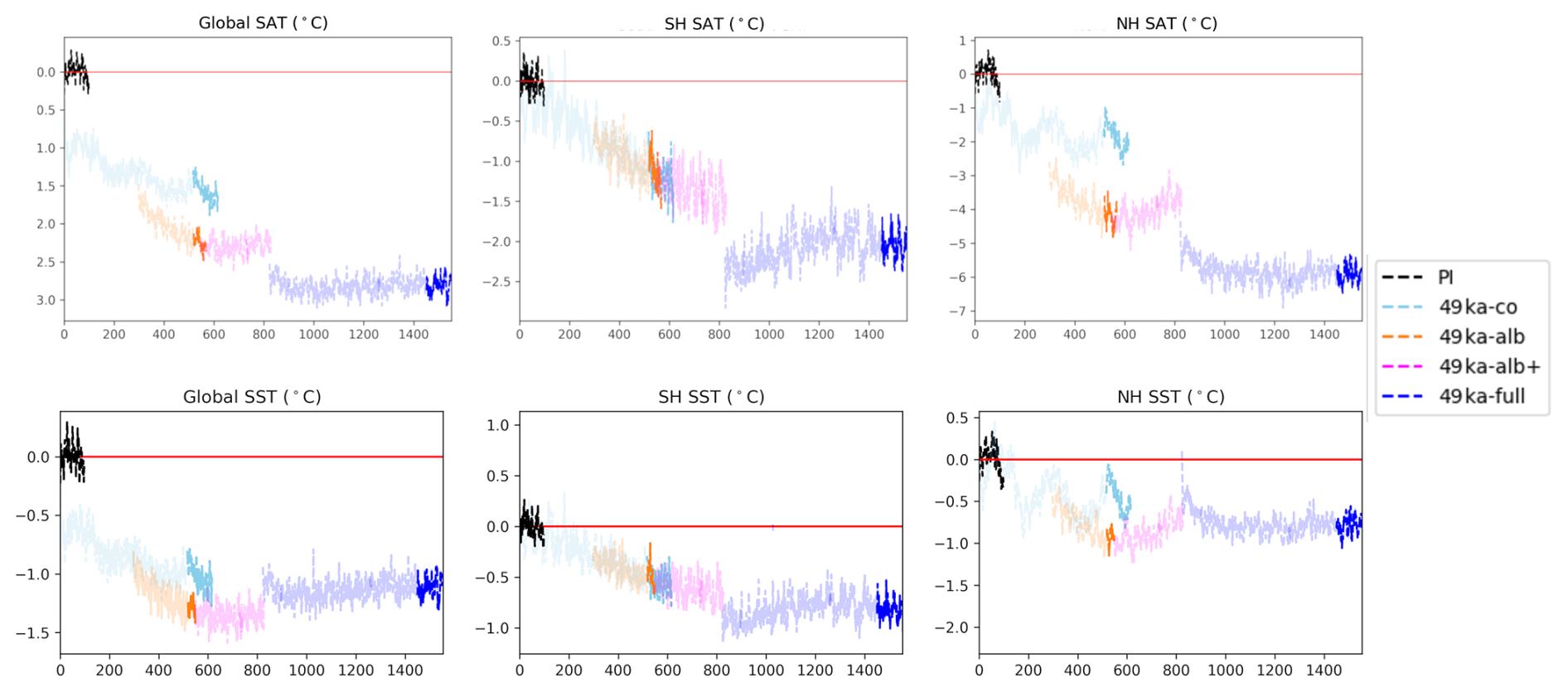
Figure A1 Time series of anomalies of annual mean (left) globally, (middle) southern hemisphere (SH), and (right) northern hemisphere (NH) averaged surface air temperature (SAT) and sea surface temperature (SST) for (black) PI, (cyan) 49ka-co, (orange)49ka-alb, and (blue) 49ka-full compared to PI. 49ka-co is orbital parameters+GHGs, 49ka-alb is 49ka-co with albedo and vegetation changes. Additional changes to 49ka-alb are shown in magenta colors (49ka-alb+). At year 547, surface salinity is gradually increased to account for the 44 m sea level drop relative to PI, to account for the increase of continental ice mass, achieving a global average increase of +0.33 psu from PI levels. At year 729, the Bering Strait is closed. The 49ka-alb+ experiment is not analysed in the manuscript. At year 824, the 49 ka topography is implemented. River runoff is adjusted to reflect the 49 ka topography at year 1258. Darker colors indicate the periods used for the analysis of time averages from each experiment. The horizontal red line is the zero line for each diagnostic shown.

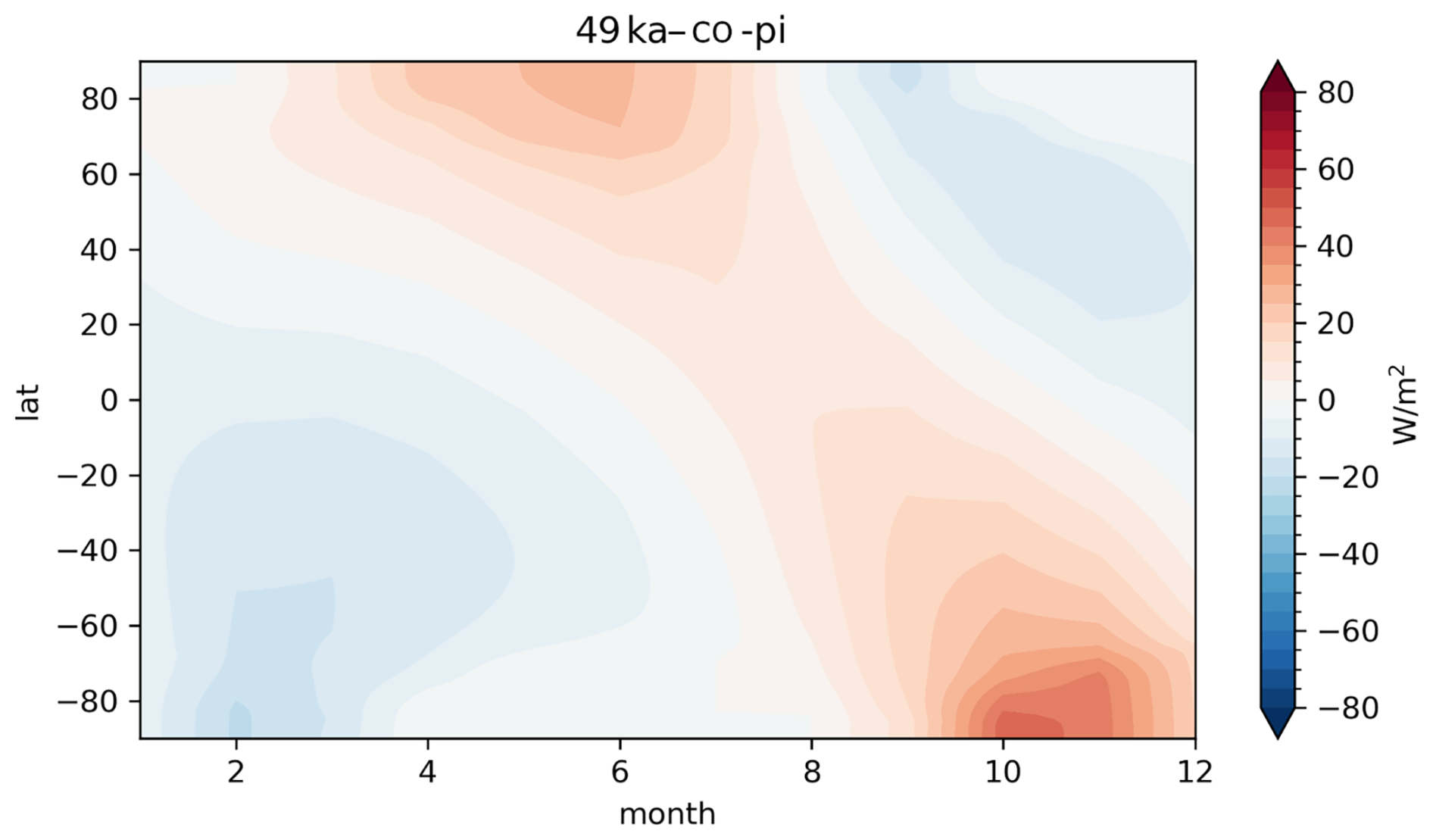
Figure A2 Insolation (Shortwave downward radiation at the top of the atmosphere) anomalies (W m⁻²) between 49 ka and PI as a function of latitude and month.

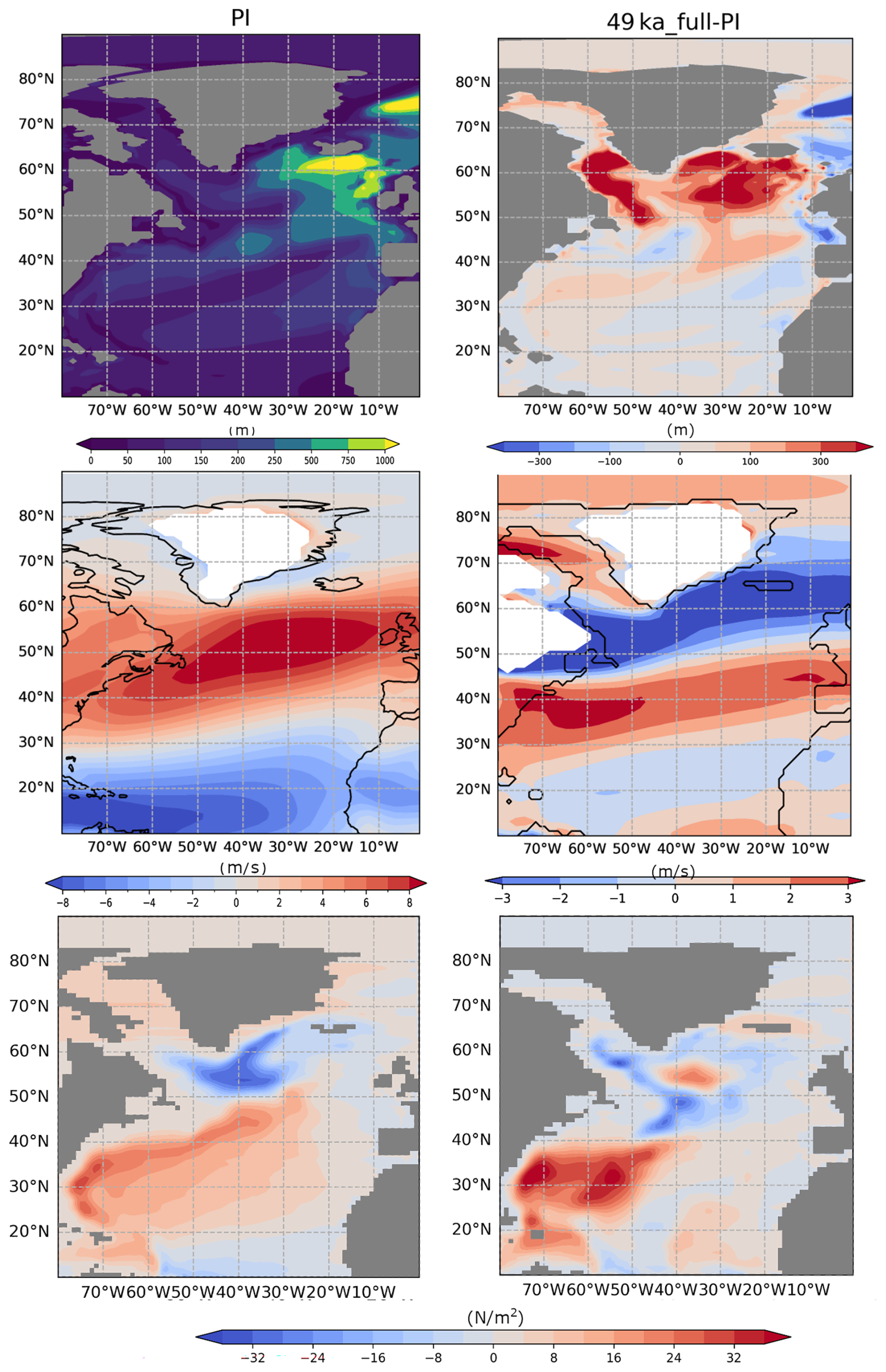
Figure A3 Winter mixed layer depth (m) (top), Zonal winds (m s⁻¹) at 850 hPa (middle), and North Atlantic gyre strength (bottom) (calculated from the barotropic streamfunction, N m⁻²) for (left) PI and (right) 49ka-full compared to PI. The white areas in the middle panel mark grid cells with continental ice, and for the 49ka-full simulation, continental outlines are shown based on the adjusted land-sea mask.

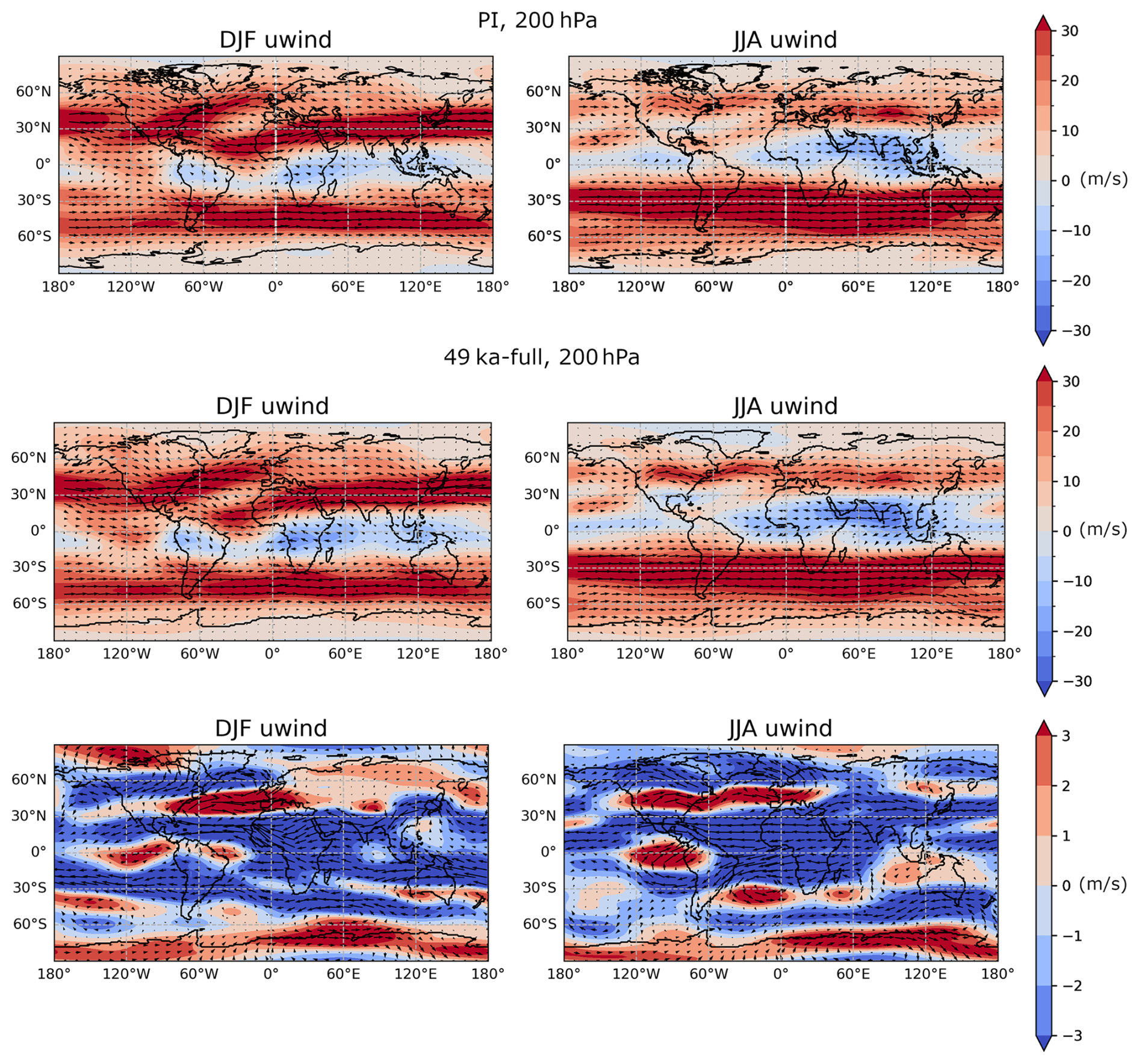
Figure A4 Zonal winds at 200 hPa (m s⁻¹) overlaid with 200 hPa wind vectors (m s⁻¹) in (left) DJF and (right) JJA for (top) PI, (middle) 49ka-full, and (bottom) 49ka-full minus PI (overlaid with 200 hPa wind vectors anomalies (m s⁻¹)).

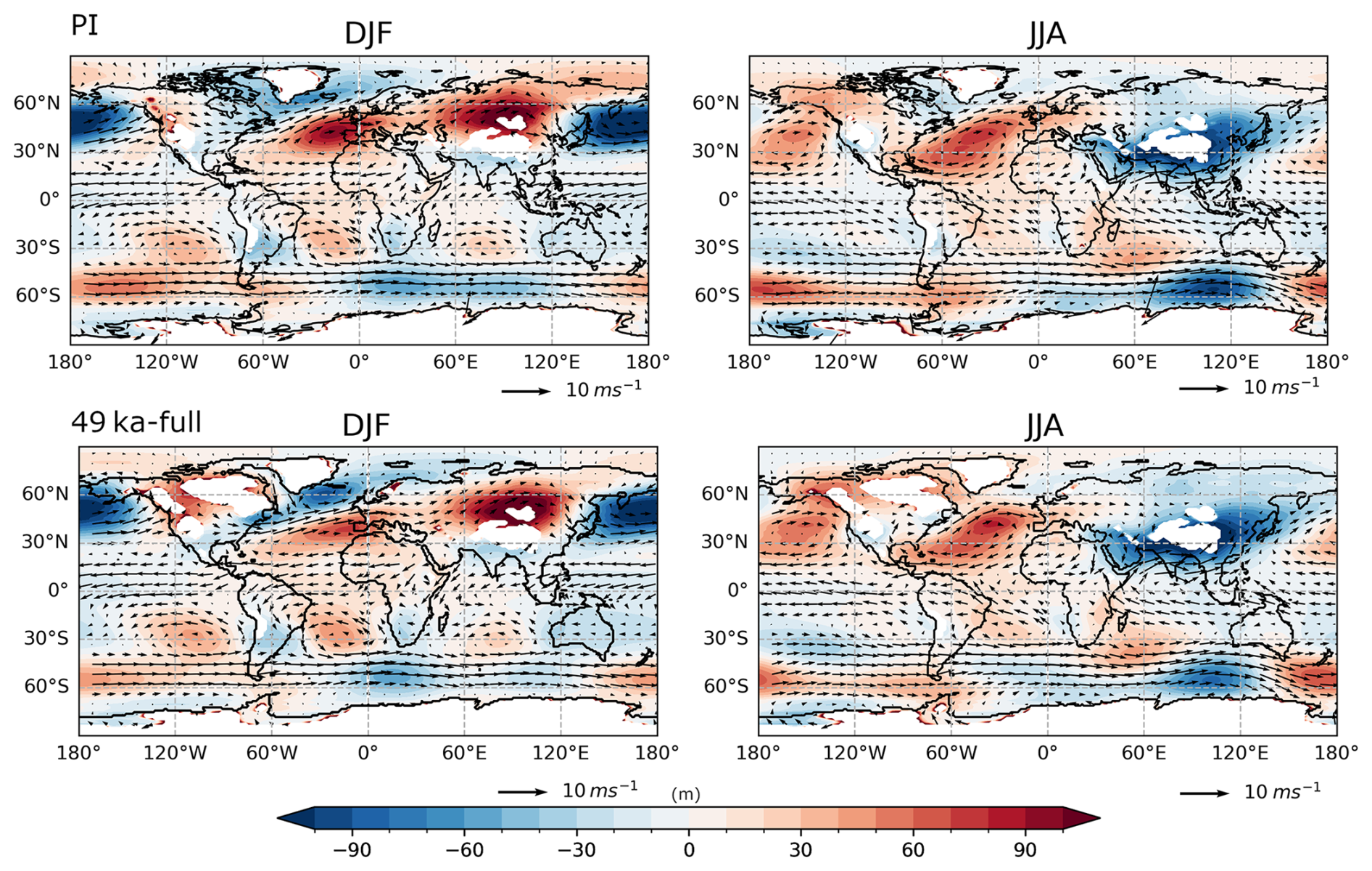
Figure A5 Geopotential height (m) at 850 hPa with zonal mean removed and overlaid with 850 hPa wind vectors in (left) DJF and (right) JJA for (top) PI and (bottom) 49ka-full.

Table A1 Global mean values for PI, 49ka-full, 49ka-alb, and 49ka-co experiments. The values in the brackets show differences from PI.