Riukojietna, a small low-altitude ice cap that may have persisted through the Holocene: evidence from combining cosmogenic multi-nuclide dating and lacustrine sediment records

Riukojietna, a small, low-altitude, low-gradient plateau ice cap in northern Sweden, has been retreating rapidly over at least the last century. Its low surface gradient implies that it should be quite sensitive to, and therefore a potentially valuable indicator of, climate change since regional deglaciation at 9.8 ka. Here, we assess its former extent and activity by combining cosmogenic nuclide measurements in bedrock (in situ ¹⁴C, ¹⁰Be, and ²⁶Al) that constrain ice-free and ice-buried conditions with indirect evidence of glacial activity from proglacial lake sediment records, complemented by historical ice thickness reconstructions. These data are the basis for subsequent forward modeling of measured cosmogenic nuclide concentrations to constrain the Holocene history of Riukojietna.

The ice cap has an outlet glacier tongue that drains to the northeast, with a bouldery moraine deposit further down valley constraining its extent at the end of the Little Ice Age (LIA, ca. 1910 CE). Five cosmogenic nuclide samples were collected: two from bedrock on the plateau adjacent to the ice cap, two from a bedrock knob protruding from the outlet glacier tongue (exposed in 2011), and one from an outcrop embedded within the LIA moraine at the outlet of the most proximal of a series of four proglacial lakes. The latter sample yielded concentrations of ¹⁴C, ¹⁰Be, and ²⁶Al consistent with continuous exposure since 8.1 ± 0.1 ka (weighted mean). Nuclide measurements in the other four samples indicate complex exposure/burial histories. Lake cores from Pajep Luoktejaure, the third of the four down-valley proglacial lakes, indicate up to three periods of glacigenic sediment deposition > 8.1 ka, from 5.4–5.0 ka, and after 1.8 ka, with intervening gyttja that indicates minimal or no glacial influence, with radiocarbon age constraints from bulk sediment and plant macrofossils.

We perform a forward modeling exercise to determine whether the cosmogenic-nuclide concentrations in the recently exposed bedrock samples are consistent with the glacial history inferred from the lake sediment record and the deglaciation age of 9.8 ka. Riukojietna persisted during the Holocene Thermal Maximum (ca. 8–5 ka), in contrast to earlier suggestions that Scandinavian glaciers vanished during the Holocene, as a result of an inferred increase in precipitation due to atmospheric circulation changes. The glacier has been in a retracted state similar or smaller than today during the late Holocene, as climate grew colder and drier. This approach combining short- and long-lived cosmogenic nuclides with lake sediments can thus provide new constraints on high-latitude Holocene glacial and paleoclimate history.

1 Introduction and Background

Mountain glaciers and ice caps are reliable indicators of regional climate change on decadal timescales because their mass balances are sensitive to changes in winter precipitation and summer ablation (Oerlemans and Fortuin, 1992; Oerlemans, 2005; Andreassen et al., 2020; Hugonnet et al., 2021; Rounce et al., 2023). Indeed, worldwide, glaciers have retreated at accelerating rates during the 20th century (Dussaillant et al., 2025; WGMS, 2025) and are projected for continued decline throughout the 21st century due to increased global temperatures (Oerlemans et al., 1998; Hock et al., 2019). Within this observed contemporary framework, this study explores the response of a small low-altitude Swedish ice cap, Riukojietna, to Holocene climate change.

A popular method to reconstruct the former extent of a glacier or ice sheet relies on exposure dating with cosmogenic nuclides in bedrock or erratics (e.g., Dunai, 2010). In glacial landscapes, the inventory of cosmogenic nuclides such as ¹⁰Be ($t_{\mathrm{1}/\mathrm{2}}$ = 1.39 Myr; Chmeleff et al., 2010; Korschinek et al., 2010) and ²⁶Al ($t_{\mathrm{1}/\mathrm{2}}$ = 705 kyr; Nishiizumi, 2004) in rock surfaces is governed by complex exposure, erosion, and ice burial histories (Gosse and Phillips, 2001; Fabel et al., 2002; Stroeven et al., 2002). When a surface is buried by > 30 m of ice, production is reduced to < 1 % of that at the surface, and radionuclides, if present, will decay at known rates to concentrations supported by production at those depths. It is not possible to resolve complex glacial histories of ice burial and exposure arising from late Pleistocene and Holocene glacier fluctuations by pairing long-lived nuclides such as ¹⁰Be and ²⁶Al since neither will decay significantly in that time frame. However, pairing a long-lived nuclide with short-lived in situ cosmogenic ¹⁴C (in situ ¹⁴C, $t_{\mathrm{1}/\mathrm{2}}$ = 5.7 kyr) enables such complex histories to be constrained. This has been demonstrated in the European Alps (Goehring et al., 2011; Wirsig et al., 2016; Schimmelpfennig et al., 2022), on Greenland and Baffin Island (Briner et al., 2014; Young et al., 2021), in Antarctica (Johnson et al., 2019; Nichols et al., 2019; Balco et al., 2023), and in Norway (Rand and Goehring, 2019).

Another common method to reconstruct past glacier extent and activity is to study proglacial lake sediment records (Karlén, 1988; Nesje et al., 2000; Rosqvist et al., 2004; Nielsen et al., 2016; Aa and Sønstegaard, 2019; Røthe et al., 2019). Typically, glacigenic sediments in a lake record (glacial flour) indicate an active glacier within the lake catchment while a prevalence of organic-rich sediments (gyttja) indicates deposition during a period of glacial inactivity or absence (Jansson et al., 2005). This is because basal sliding by a warm-based glacier is required for a glacier to erode its substrate and produce glacial flour. However, several other factors influence the sedimentation rate in proglacial lakes, such as hydrological regime, intermediate sediment storage capacity, and the activity of other geomorphological processes within the catchment (Leonard, 1986; Rubensdotter and Rosqvist, 2003; Jansson et al., 2005). In a setting with a sequence of lakes acting as sediment traps, glacigenic lake sedimentation may constrain the ice extent (Jansson et al., 2005; Nesje, 2009).

Climate reconstructions based on vegetation development and lake sediment proxy records indicate that the climate in northern Sweden warmed rapidly and that conditions were relatively wet (Shemesh et al., 2001; Sjögren and Damm, 2019) when the Fennoscandian Ice Sheet (FIS) melted (Kullman and Öberg, 2015; Sjögren, 2021). Even warmer but also drier summer conditions characterize the so-called Holocene Thermal Maximum (HTM; ∼ 8–5 ka; Barnekow, 2000; Seppä et al., 2005; Sjögren, 2021; Wastegård, 2022). Based on sediment stratigraphies in proglacial lakes, Karlén (1976, 1981, 1988) proposed that some Swedish glaciers advanced during this time while others may have melted away, in line with records from some Norwegian glaciers (Bjune et al., 2005; Nesje et al., 2008; Nesje, 2009). Proglacial lake records show that glacier activity generally increased in response to an overall cooling trend after 5 ka, a progression that is documented across the Arctic (Karlén et al., 1995; Matthews and Dresser, 2008; Kaufman et al., 2009; Larocca and Axford, 2022). The latest period of glacier reactivation was during the Little Ice Age (LIA; 1500–1900 CE), and evidence for this is rich compared to earlier periods (Grove, 2004; Matthews and Briffa, 2005).

Based on lichenometric dating of end moraine ridges, Karlén (1988) inferred that most Swedish glaciers reached their maximum Holocene position sometime during the 18th century and, supported by the oldest photographic evidence (Svenonius, 1910), again as late as ca. 1910 CE. Geomorphic evidence of earlier Holocene advances was potentially eradicated during this time (Jansson et al., 2005). Sediments from proglacial lakes therefore constitute the best continuous archive of Holocene glacier activity.

Here, we aim to constrain the former size and activity of Riukojietna (Sámi: Rivgojiehkki), a rapidly retreating ice cap located in northern Sweden (Fig. 1). We do this by combining evidence for ice-free conditions and ice-burial durations from cosmogenic nuclide chronometry (in situ ¹⁴C, ¹⁰Be, ²⁶Al) and evidence of glacial extent and activity derived from proglacial lacustrine records, complemented with ice-cap reconstructions based on historical records. This allows us to present the first full Holocene glacial history of a Swedish glacier based on multi-proxy records, and evaluate its sensitivity to Holocene climate change.

Figure 1 (a) Map showing deglacial isochrons of the Fennoscandian Ice Sheet (Stroeven et al., 2016) in 100-year intervals around the location of Riukojietna (box with white dot: panel b). (b) European Union Digital Elevation Model (EU-DEM) of northern Sweden/Norway depicting the location of glaciers, including Riukojietna (box: Fig. 2a). The numbers on the contours are deglacial isochrons in cal ka BP (Stroeven et al., 2016). Modified from Koester (2023).

2 Study site

Riukojietna is a small, thin (thickness < 100 m), polythermal ice cap covering a plateau on the Swedish-Norwegian border (Fig. 2). This ice cap is ideal for studying Late Pleistocene to Holocene glacier fluctuations using cosmogenic nuclides and lake sediments for two reasons. First, the ice cap rests on quartz-rich bedrock of the Köli Nappe which allows for the application of multiple nuclides, including ¹⁰Be, ²⁶Al, and in situ ¹⁴C. In contrast, most glaciers in northern Sweden are situated in the higher alpine areas where amphibolite and metadolerite bedrock of the Seve Nappe dominates (Andréasson and Gee, 1989; Bergman et al., 2012). Second, a thin and blocky till cover, gentle slopes, and an absence of sediment-rich landforms in the catchment implies that glacial flour is the dominant source of minerogenic material in downstream lakes. As such, we expect lake records from the catchment to primarily reflect fluctuations in glacier activity and extent.

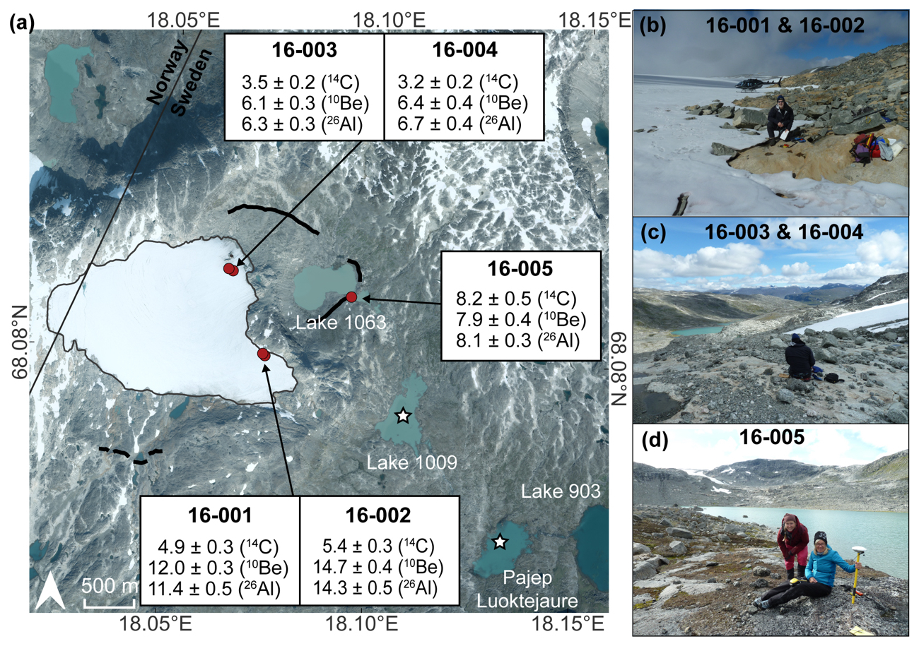
Figure 2 (a) Google Earth satellite image (2018; Map data: Google, © 2025 CNES/Airbus) of the Riukojietna ice cap depicting the location of bedrock samples (red circles). Simple exposure ages with internal uncertainties (in ka) are shown in white boxes. Thick black lines depict the location of Late Holocene moraines. White stars depict lakes that have been cored downstream of the ice cap. (b) Two bedrock samples collected directly adjacent to the ice cap (1290 m a.s.l.). (c) Two bedrock samples collected from a bedrock knob that was exposed in 2011 (1240 m a.s.l.). (d) One bedrock sample collected adjacent to Lake 1063 outlet (1064 m a.s.l.). Modified from Koester (2023).

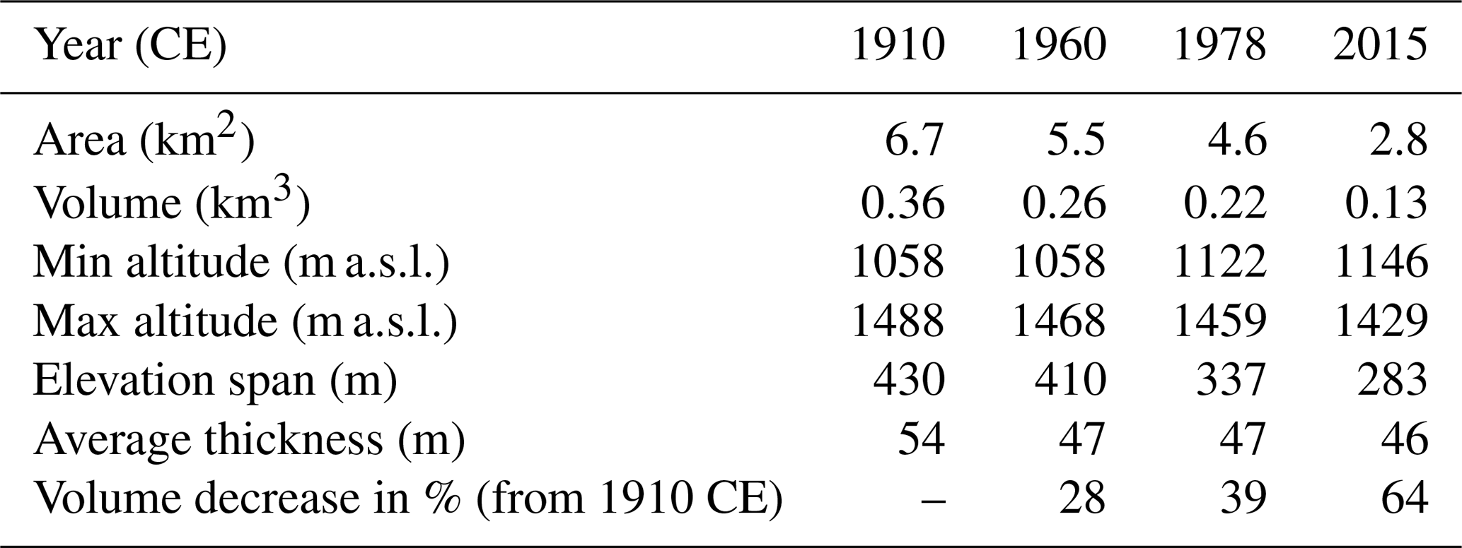
Riukojietna had an area of 5.5 and 4.6 km² when surveyed from 1960 and 1978 aerial photographs, respectively (Rosqvist and Østrem, 1989; Table 1). However, the ice cap has continued to shrink, covering a mere 2.8 km² and thinned to span only 283 m vertically between the ice divide and the snout in 2015 (Table 1). The ice cap flows radially outwards from its highest point and is impounded by bedrock ridges to the south and northeast. Currently, Riukojietna has one outlet glacier tongue that terminates on a steep rise to the northeast (Fig. 2). The position of this tongue has been mapped since 1963 and the glacier mass balance has been monitored annually since 1986 revealing high sensitivity to changes in summer temperature and winter precipitation (WGMS, 2025). Two topographic maps were constructed based on aerial photography from 1960 and 1978 showing ice cap surface topography and extent (Rosqvist and Østrem, 1989). The eastern terminus calved into Lake 1063 (Fig. 2) before 1960 but retreated up-valley after 1975. Ice volume has been decreasing significantly during the 20th century (Table 1) due to a dominantly negative annual mass balance (WGMS, 2025). Because it is relatively low-elevation and spans an unusually narrow elevation interval compared to most valley glaciers in the region, Riukojietna is regarded to be highly sensitive to climate change (Rosqvist and Østrem, 1989).

Table 1 Riukojietna area, thickness, and volume reconstructions since the LIA (Carl-Anton Wahlström, 2016, A century of volume reduction of a small ice cap; Riukojietna northern Sweden, unpublished, MSc thesis, Department of Physical Geography, Stockholm University).

Four lakes on the eastern side of the ice cap act as a series of traps for sediment derived from glacial erosion. Ordered by decreasing elevation (in m a.s.l.), they are lakes 1063, 1009, Pajep Luoktejaure (913; where “Pajep” means upper and “jaure” means lake – so Upper Luokte lake), and Vuolep Luoktejaure (903) (or Lower Luokte lake, which is only partially visible in Fig. 2). Lakes at this latitude and altitude are generally ice-covered from October to June (Rosqvist et al., 2004). From the variations in relative densities and organic content in sediment cores from Lake 1009 and Pajep Luoktejaure, Karlén (1981, 1988) proposed that Riukojietna was inactive and small, or disappeared, between 10.9 ± 0.4 (Si-2860) and 2.7 ± 0.1 (Si-2859) cal ka BP (re-calibrated bulk sediment samples using the online CALIB Radiocarbon Calibration v 8.2; Stuiver and Reimer, 1993; Reimer et al., 2020) and that the ice cap subsequently reactivated.

The relatively prominent lateral/end moraine sequence consisting of large boulders located to the northeast and east of Lake 1063 (Fig. 2) indicates that the ice cap advanced to this position at least once during the Holocene. A depositional age of ca. 1910 CE was inferred for this ridge (Pohjola et al., 2005) based on lichenometry of Rhizocarpon geographicum and Rhizocarpon alpicola (Karlén, 1973), which is similar to other lichenometry-dated LIA moraines in the region (Karlén, 1976; Karlén and Denton, 1976). A less prominent moraine ridge indicates that the glacier once extended down the southwestern slope of the plateau (Fig. 2). A glacially molded plateau surface extends from the current ice cap margin towards the southeast, indicating a possible earlier extension direction of the ice cap towards Lake 1009 (Koester, 2023).

3 Methods

We combine cosmogenic nuclide chronometry, lacustrine sediment records, historic ice cap reconstructions, and modeling of complex exposure histories to evaluate the Holocene history of Riukojietna (Koester, 2023). Each method is described in detail below.

3.1 Cosmogenic nuclide sampling and analysis

We collected five granitic bedrock samples with angle grinder, hammer, and chisel from three locations near Riukojietna in August 2016 and measured concentrations of in situ ¹⁰Be, ²⁶Al, and ¹⁴C (Fig. 2, Table 2). Two samples were collected from the base of a small bedrock ridge immediately adjacent to the ice cap (< 2 m from the modern ice; Riuko-16-001 and 16-002). Two samples were taken from a bedrock knob protruding through the outlet glacier tongue that became exposed in 2011 (Riuko-16-003 and 16-004). In the following, we collectively refer to these two sites as “ice-marginal bedrock”. The last sample was collected from a bedrock outcrop adjacent to the outlet of Lake 1063 (Riuko-16-005), in the following referred to as the “lake outlet sample”. The bedrock outcrops in line with the LIA moraine and constitutes the subglacial meltwater outlet of Riukojietna at that time.

Table 2 Sample information and measured cosmogenic nuclide concentrations.

We separated quartz at the Purdue Rare Isotope Measurement Laboratory (PRIME Lab) using standard mineral separation procedures (https://www.physics.purdue.edu/primelab/labs/mineral-separation-lab/procedure.php, last access: 28 April 2026). Samples were crushed, sieved to 250–500 µm, and magnetic minerals removed using a Carpco magnetic separator. Micas and feldspars were removed with froth flotation, and the remaining quartz separate was subsequently leached in weak hydrofluoric (HF) and nitric acids (HNO₃) to remove meteoric ¹⁰Be (Kohl and Nishiizumi, 1992). Quartz purity was assessed with inductively coupled plasma–optical emission spectrometry (ICP-OES) at PRIME Lab (Al target: < 200 ppm). Riuko-16-002 and Riuko-16-005 had high Al and Na contents, indicating the presence of feldspars, and were therefore subjected to an additional separation step using heavy liquids and etching in weak acids. We have never observed any demonstrable effects from froth flotation on PRIME Lab in situ ¹⁴C measurements using these quartz purification procedures, thus no additional steps were taken (e.g., Nichols and Goehring, 2019).

Beryllium and aluminum were extracted at PRIME Lab following the procedures outlined in Andersen et al. (2020). Beryllium samples were spiked with ∼ 0.26 mg of Be carrier and aluminum samples were spiked with 0.9–1.3 mg of Al carrier if they did not contain enough native Al before digestion in HF (target ∼ 1.5 mg Al). The samples were prepared in one batch with a procedural blank and an aliquot of the intercomparison material CoQtz-N (Binnie et al., 2019). Be and Al were separated through anion and cation column chromatography, precipitated, oxidized, mixed with niobium powder, and pressed into cathodes for measurement. Isotopic ratios (¹⁰Be $/$ ⁹Be and ²⁶Al $/$ ²⁷Al) were measured by accelerator mass spectrometry (AMS) at PRIME Lab.

Carbon-14 was extracted at PRIME Lab using the automated Carbon Extraction and Graphitization System described by Lifton et al. (2023) and following procedures modified from that publication. Twenty grams of lithium metaborate (LiBO₂) flux is first degassed for 1 h at 1100 °C in a reusable Pt-Rh boat (90 % Pt, 10 % Rh) in ∼ 6.67 kPa of Research Purity O₂, allowed to cool overnight under vacuum, and then approximately 5 g of sample quartz is evenly distributed over the solidified LiBO₂. The sample is then combusted at 500 °C for one hour in ∼ 6.67 kPa of Research Purity O₂ to remove atmospheric/organic contaminants, and the system is evacuated. Approximately 6.67 kPa of Research Purity O₂ is then added to the system, and the sample is heated to 1100 °C for three hours to release any trapped carbon species. All evolved C species are oxidized to CO₂ by passing the process gas over 2 mm quartz beads at ∼ 950 °C. After extraction, the evolved gas is collected in a coil trap cooled with liquid nitrogen, purified using a variable temperature trap at −145 °C and passed over Cu mesh and Ag wool held at 600 °C to remove contaminants, before volume measurement and dilution with ¹⁴C-free CO₂ to the equivalent of ∼ 300 µg C. Finally, a ca. 9 µg C split is collected for stable C isotopic measurement, and the remaining sample is reduced to graphite in Research Purity H₂ over an Fe catalyst before packing into a cathode for AMS measurement (e.g., Santos et al., 2004, 2007).

Sample ¹⁴C $/$ ¹³C ratios were measured by AMS relative to Oxalic Acid II (NIST-4990C) at Purdue University. Stable carbon isotopic ratios were measured at the University of California Davis Stable Isotope Facility using isotope ratio mass spectrometry (e.g., Lifton et al., 2023). The ¹⁴C concentration is calculated from the measured ¹⁴C $/$ C_total after subtracting out representative procedural background ¹⁴C (Hippe and Lifton, 2014).

We use the primary CRONUS-Earth global calibration spallation production rates for ¹⁰Be (3.9 ± 0.3 at g⁻¹ yr⁻¹), ²⁶Al (28.5 ± 3.1 at g⁻¹ yr⁻¹) and in situ ¹⁴C (12.8 ± 0.9 at g⁻¹ yr⁻¹) to calculate exposure ages and model ice burial and erosion histories (Lifton et al., 2014, 2016; Borchers et al., 2016; Phillips et al., 2016). The in situ ¹⁴C production rate also includes the Young et al. (2014) in situ ¹⁴C calibration dataset (Koester and Lifton, 2023, 2024). All calculations utilize nuclide-specific LSDn scaling (Lifton et al., 2014, 2016) and the muon production formulation from Balco (2017). Simple exposure ages (i.e., assuming continuous exposure with no erosion or burial) and 1σ uncertainties were calculated using the online University of Washington cosmogenic calculator, v.3 (wrapper script 3.0.2, constants: 26 August 2024, muons: 1A; Balco et al., 2008; https://hess.ess.washington.edu/math/, last access: 28 April 2026), with in situ ¹⁴C production rates calibrated using the above datasets.

3.2 Lacustrine sediment cores

Pajep Luoktejaure has a relatively even bathymetry with one deeper section (12 m) in its northern part. We retrieved a deep core (1995) and five surface and deep cores (PL1–PL5) from the deepest part of the lake in April 1995 and April 1998, respectively. We used a gravity corer to retrieve an undisturbed surface sample (top 25 cm; PL3) and a modified Livingstone piston corer (90 mm diameter) for the others (1995; PL1, 2, 4, and 5). Visual inspection and results from measurements of loss-on-ignition (LOI), determined at 550 °C with 1 cm resolution, for PL1–PL4 show the same general stratigraphy for common sections (PL5 remains unopened, for reference). PL1-169 is the longest core (down to 169 cm below the lake floor) and the only one representing the early phase of lake development. The composite stratigraphic description of Pajep Luoktejaure is based on this core and surface core PL3-25.

Sedimentary structures and grayscale densities of cores PL1-169 and PL3-25 were determined by X-ray radiography (Rubensdotter and Rosqvist, 2003; Rosqvist et al., 2004). Line transects (1 mm width) of grayscale density values were taken at a resolution of 0.3 mm. In this study, grayscale density is merely used to identify areas of lamination. Grain size distribution was analyzed in a SediGraph 5100 on 1 cm slices of specific sedimentary structures (i.e., finely laminated minerogenic sections at 115–117 and 8–10 cm depths in core PL1-169, and replicated by results from finely laminated minerogenic sections at 128–131 and 6–9 cm depths in core PL2-133; Fig. S1 and Table S1 in the Supplement).

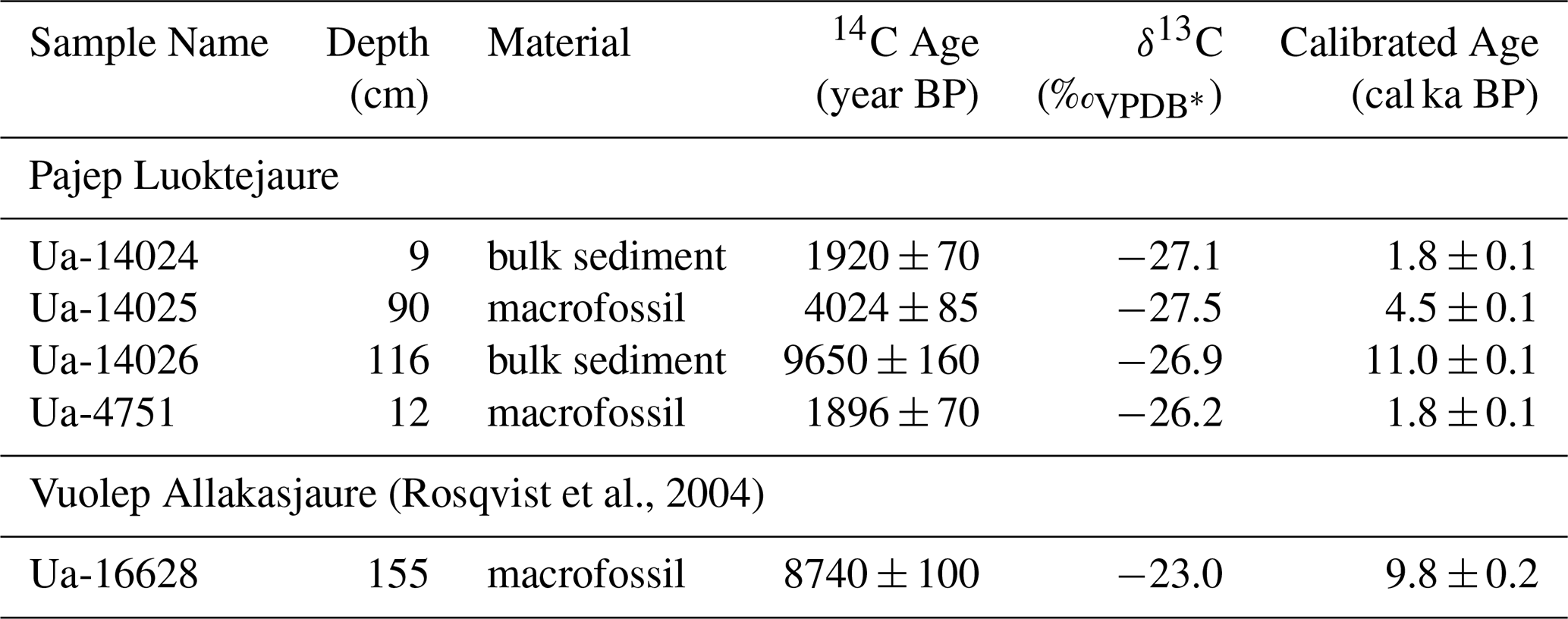
Age control is provided by four samples from Pajep Luoktejaure; three AMS ¹⁴C-dates from core PL1-169 and one from near-surface sediments in the core of 1995 (Table 3). We also used a basal date derived from a terrestrial plant macrofossil from nearby lake Vuolep Allakasjaure to help constrain the timing of deglaciation (Table 3). The samples were radiocarbon dated at the Ångström Laboratory, Uppsala University, and converted to calendar ages using the IntCal20 calibration curve (Reimer et al., 2020). Three of the radiocarbon constraints were used to derive an age–depth model using the Bayesian accumulation age-modelling software of Blaauw and Christen (2011; Fig. S2).

Table 3 Radiocarbon chronology for Pajep Luoktejaure. Three radiocarbon dates were derived from core PL1-169 at 116 cm depth (1 cm bulk sample), 90 cm depth (terrestrial macrofossil), and 9 cm depth (1 cm bulk sample). The latter replicated the date from a 12 cm depth terrestrial macrofossil sample of the same stratigraphic unit in the 1995 core from Pajep Luoktejaure. The basal bulk sediment age was replicated with a terrestrial macrofossil date from the same stratigraphic position (first radiocarbon accumulation after deglaciation) from nearby lake Vuolep Allakasjaure (12 km distance; Rosqvist et al., 2004; Fig. 1b). Calibrated ages derived using CALIB Radiocarbon Calibration v 8.2 (http://calib.org/calib/, last access: 28 April 2026; Stuiver and Reimer, 1993; Reimer et al., 2020).

* Measured relative to the Vienna Peedee Belemnite standard

3.3 Modern ice thickness reconstructions, bed topography, and volume calculations

Detailed ice surface topographic maps were constructed from aerial photographs taken in 1960 and 1978 to determine the average mass balance of Riukojietna (Rosqvist and Østrem, 1989). These two maps, reproduced at 1:10 000 in the back sleeve of the Journal issue featuring Rosqvist and Østrem (1989), were scanned and georeferenced in QGIS software to derive the ice-cap surface elevation during these years. The ice-cap topography was additionally mapped during the summer of 2014 and spring of 2015 using two differential GPS (dGPS) rover units. The subglacial bedrock topography was constrained with ground penetrating radar (GPR) towed behind a snowmobile in the springs of 2011, 2012, and 2015 (Fig. S3). We use these data sources to track ice cap area and volume changes relative to a 2 m-resolution LiDAR digital elevation model (DEM) from 2015 (Fig. S3).

The elevations of fixed bedrock points on the 1960 and 1978 maps were compared to the recent LiDAR DEM to evaluate their accuracies, and differences were calculated. These differences were interpolated using kriging in Surfer 11 to create misfit values across the glacier surface. The resulting spatial pattern of misfit is used to correct the altitudes derived from the 1960 and 1978 maps to better match ice surface elevations to the 2015 LiDAR DEM (Fig. S4).

The perimeter of the presumed LIA glacial extent (1910 CE) was mapped from the 1960 and 1978 orthophotos and integrates the location of the eastern terminal moraine. As there are no moraines limiting previous extents on the western side, we assumed a 50–100 m more expanded glacier relative to its extent in 1960. The 1910 CE ice surface was calculated for the central flow line (Fig. S5) using the reconstructed bed topography, a target maximum elevation of 1490 m a.s.l. based on a summit ice thickness of ca. 93 m estimated by Pohjola et al. (2005), and an adjustable yield stress following Benn and Hulton (2010). The surface elevations were interpolated in Surfer 11 using kriging to create an LIA ice surface reconstruction. For each of the four time slices, Surfer 11 was used to calculate the volume and average ice thickness of Riukojietna using the difference between the ice surface DEM and the bed topography DEM (Table 1).

3.4 Modeling complex exposure histories

We explore potential effects of temporal variations in ice cap thickness on our ice-marginal bedrock cosmogenic nuclide inventories (Riuko-16-001 to 16-004) using a Lagrangian forward modeling framework (e.g., Knudsen et al., 2019) implemented in MATLAB. This model predicts the post-LGM time evolution of ¹⁰Be, ²⁶Al, and ¹⁴C concentrations in bedrock during subaerial exposure and when either completely (ice > 30 m thick) or incompletely shielded beneath thin ice (< 30 m thick) from both spallogenic and muogenic production, while allowing for subglacial erosion. Modeling details are provided in Sects. S1–S3 in the Supplement.

4 Results

4.1 Cosmogenic nuclide concentrations and simple exposure ages

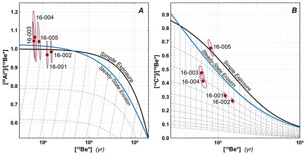
The ¹⁰Be concentrations in bedrock samples Riuko-16-001 to 16-005 range from 8.8 ± 0.4 × 10⁴ to 2.2 ± 0.1 × 10⁵ atoms g⁻¹, while the ²⁶Al concentrations range from 6.4 ± 0.3 × 10⁵ to 1.5 ± 0.1 × 10⁶ atoms g⁻¹ (Tables 2, S2; Koester, 2023). Measured in situ ¹⁴C concentrations range from 1.3 ± 0.1 × 10⁵ to 2.3 ± 0.1 × 10⁵ atoms g⁻¹ (Tables 2, S3; Koester, 2023). The corresponding simple exposure ages range between 3.2 ± 0.2 and 8.2 ± 0.5 ka for in situ ¹⁴C, 6.3 ± 0.3 and 14.3 ± 0.5 ka for ²⁶Al, and 6.1 ± 0.3 and 14.7 ± 0.4 ka for ¹⁰Be (Fig. 2; Tables S2–S4). When plotted on a two-isotope diagram, the ¹⁰Be-²⁶Al results of all five bedrock samples overlap with the simple exposure line at 1σ (Fig. 3a). In contrast, the ¹⁴C-¹⁰Be two-isotope diagram shows that only sample Riuko-16-005 overlaps the simple exposure line, indicating continuous exposure since deglaciation for that sample (Fig. 3b). All simple exposure ages for this sample agree within 1σ external (and internal) uncertainty (Fig. 2). Using external uncertainties, the weighted mean and the larger of either the standard error in inverse-error-weighted mean, or the inverse-error-weighted average variance (Bevington and Robinson, 2003) yields 8.0 ± 0.1 ka, while the straight mean and standard deviation yields 8.1 ± 0.1 ka. As these values are not significantly different, we take the straight mean ¹⁴C-¹⁰Be-²⁶Al exposure age of 8.1 ± 0.1 ka (1σ) as the deglacial age for that location.

Figure 3 (A) Two-isotope diagram of normalized ²⁶Al $/$ ¹⁰Be concentration ratio vs. normalized ¹⁰Be concentration. Ellipses show 2σ uncertainty. Normalization (indicated by ^*) is to site production rates, hence the unit of [¹⁰Be^*] is year. (B) Two-isotope diagram of normalized in situ ¹⁴C $/$ ¹⁰Be concentration ratio vs. normalized ¹⁰Be concentration. Burial isochrons (dashed lines) are calculated relative to the simple exposure curve. Burial isochron spacing is 500 kyr in panel (A), and 2 kyr in panel (B). Near-vertical dot-dashed lines are decay trajectories followed during burial, plotted in panel (A) for every fifth age in a logarithmic array of 100 ages generated from 100 to 10⁷ years that lie within the x-axis limits, and in panel (B) for every other age in a logarithmic array of 100 ages generated from 100 to 2 × 10⁵ years that lie within the x-axis limits.

The remaining samples (Riuko-16-001 to 16-004) plot in the complex exposure field of the ¹⁴C-¹⁰Be two-isotope diagram (Fig. 3b). Because simple ¹⁰Be and ²⁶Al exposure ages for the same samples overlap within 1σ, we focus dominantly on the ¹⁰Be and ¹⁴C values in the remainder of the paper. The highest elevation site, adjacent to the current ice cap margin (∼ 1290 m a.s.l.; Riuko-16-001 and 16-002), has the oldest simple ¹⁰Be (¹⁴C) exposure ages of 12.0 ± 0.3 (4.9 ± 0.3) and 14.7 ± 0.4 (5.4 ± 0.3) ka, respectively (Fig. 2). The two samples collected on the recently emerged bedrock knob at ∼ 1240 m a.s.l. (Riuko-16-003 and 16-004) have younger ¹⁰Be (¹⁴C) simple exposure ages of 6.1 ± 0.3 (3.5 ± 0.2) and 6.4 ± 0.4 (3.2 ± 0.2) ka, respectively – internally consistent for each nuclide but disagreeing between nuclides (Koester, 2023).

4.2 Lacustrine records

The bottom of core PL1-169 from 169 to 116 cm depth is characterized by homogenous glacial silt and clay (Fig. 4b) with LOI less than 2 %. Between 116 and 107 cm depth, sediments are finely laminated silt and clay with LOI less than 10 %. Laminations become more diffuse between 107 and 95 cm depth and LOI values increase, reaching as high as 16 % at 98 cm depth. A drop in LOI to 7 % at 93 cm is caused by an influx of minerogenic matter. Homogenous gyttja with up to 26 % LOI characterizes the sediments between 90 and 10 cm depth. The uppermost 10 cm of PL1-169 consist of finely laminated silt and clay with high density and low LOI (between 5 % and 8 %). Results from grain size distribution analyses show indeed that the sampled sections consist of silt and minor amounts of clay (> 85 % silt/clay; i.e. < 63 µm; Table S1).

Figure 4 Stratigraphy and loss on ignition (LOI %) from (a) surface gravity core PL3-25 and (b) Livingstone piston core PL1-169 in Pajep Luoktejaure (Fig. 2a). High LOI indicates high organic content, interpreted as relatively low glacial activity, while low LOI indicates low organic content associated with a relatively active glacier and minerogenic influx. Core PL1-169 has 3 radiocarbon tie points (in cal ka BP; Table 3). (c) Composite core of LOI record versus age, where 1–13 cm are from PL3-25 and 13–130 cm are from PL1-169. Age vs. depth for PL1-169 below 130 cm is poorly constrained. (Fig. S2). In this conversion we replaced the basal bulk sediment age of 11.0 ± 0.1 cal ka BP with a terrestrial macrofossil date of 9.8 ± 0.2 cal ka BP from the same stratigraphic position (first radiocarbon accumulation after deglaciation) from nearby lake Vuolep Allakasjaure (Table 3). Blue fields indicate our inferred periods of glacier activity. The lowest field is informed by the cosmogenic nuclide retreat age of Riukojietna from the outlet of Lake 1063 at 8.1 ± 0.1 ka. The youngest period of inferred glacier activity is informed by the oldest ages of glacier reactivation of 1.8 ± 0.1 cal ka BP (on macrofossil and bulk sediment; Table 3) and final retreat from the LIA moraine at 1910 CE. During the mid-Holocene short period of glacier activity between 5.4 and 5.0 cal ka BP, LOI values are on-par with the previous and subsequent periods of inferred glacier activity.

Surface core PL3-25 records the intact uppermost 25 cm of the stratigraphy in Pajep Luoktejaure (Fig. 4a). Its sedimentary structure is similar to PL1-169 in the overlapping interval. Well-preserved laminations are observed between 19 and 3 cm. The topmost 3 cm of the core displays high LOI (up to 17 % at the surface). No laminations are detectable in these non-compacted organic surface sediments.

Three radiocarbon dates were obtained from PL1-169, with the oldest (116 cm depth; 11.0 ± 0.1 cal ka BP; 2 % LOI) and youngest (9 cm depth; 1.8 ± 0.1 cal ka BP; 14 % LOI) ages derived from bulk sediment and the intermediate age (90 cm depth; 4.5 ± 0.1 cal ka BP) derived from a terrestrial plant macrofossil (Table 3). An additional radiocarbon date of a terrestrial macrofossil at 12 cm depth in the 1995 core, also representing the first deposition of late Holocene laminations in the core, replicates the bulk sediment age at 9 cm depth of 1.8 ± 0.1 cal ka BP (Table 3). The basal radiocarbon age, from bulk sediment with only 2 % organic content, is much older than the expected regional ∼ 9.8 cal ka BP deglaciation age (Fig. 1b) of Stroeven et al. (2016). Therefore, we adopt the basal sediment age from nearby lake Vuolep Allakasjaure (Fig. 1b; ∼ 12 km NE of Pajep Luoktejaure) of 9.8 ± 0.2 cal ka BP derived from a terrestrial macrofossil in the same stratigraphic position, that is, representing the first radiocarbon accumulation after deglaciation (Table 3; Rosqvist et al., 2004). Together with the two youngest radiocarbon ages (at 90 and 9 cm depth) and a sediment surface age of −48 BP (i.e., 1998 CE) they create the four tie points constraining the age-depth model (Fig. S2). To provide a composite record we spliced the core PL3-25 LOI record representing the top 13 cm of the sediment record into the PL1-169 LOI record (Fig. 4c). The average sedimentation rate of the upper laminated section is ∼ 0.1 mm yr⁻¹ if the uppermost 3 cm corresponds to the time since the glacier retreated from the moraine at Lake 1063 at the end of the LIA. The sedimentation rate of the organic section (90–9 cm) is ∼ 0.3 mm yr⁻¹.

4.3 Ice thickness and volume reconstructions

Ice thickness reconstructions for the past century are shown in Fig. 5. At the end of the LIA, Riukojietna covered an area of 6.7 km² and had an estimated volume of 0.36 km³ (Table 1). Ice extent and volume have decreased by > 58 % and > 64 %, respectively, between 1910 CE and 2015 (Table 1; Fig. 5). Based on these reconstructions, we estimate that the ice thickness above our two ice-marginal cosmogenic sample locations (Riuko-16-001 to 16-004) started at 33–35 m one century prior to exposure (Table S5; Koester, 2023).

Figure 5 Ice thickness reconstructions for Riukojietna from 1910 CE, 1960, 1978, and 2015 with respect to the maximum extent of 1910 CE (LIA extent). The 40 m ice thickness contour is shown in dashed grey. Sample sites are shown as red dots. Figure modified from Wahlström (2016; A century of volume reduction of a small ice cap; Riukojietna northern Sweden, unpublished, MSc thesis, Department of Physical Geography, Stockholm University).

5 Discussion

5.1 Constraints on the Holocene history of Riukojietna from the lake outlet sample

The cosmogenic nuclide results offer constraints on the dimensions, including the minimum thickness of Riukojietna, through the Holocene (Koester, 2023). The agreement between ¹⁴C-¹⁰Be-²⁶Al simple exposure ages at 1σ for the lake outlet sample (Riuko-16-005; 1064 m a.s.l.) indicates continuous exposure at that site since deglaciation following erosional resetting of the surface. Thus, this result establishes that Riukojietna did not cover or expand beyond the Lake 1063 outlet sampling site after 8.1 ± 0.1 ka (mean of all three nuclide ages; Fig. 2). The result also reveals that the FIS, or Riukojietna, eroded sufficient bedrock at that site to remove any cosmogenic nuclide inventory produced prior to the Last Glacial Maximum (LGM).

5.2 Constraints on the Holocene history of Riukojietna from lacustrine sediments

Pajep Luoktejaure receives meltwater coming from the northeastern active outlet of Riukojietna (Fig. 2). Lakes 1063 and 1009 in its drainage system act as sediment traps. This will have a damping effect on sedimentary responses in Pajep Luoktejaure to changes in the activity and extent of Riukojietna.

Meltwater from the southeastern tongue of Riukojietna also enters Lake 1009 before it reaches Pajep Luoktejaure (Fig. 2). However, based on thermistor measurements in 1986 (Pohjola et al., 2005), the ice cap dome, and by inference its thin low-gradient southeastern tongue, were shown to be cold-based, which means that sub-glacial erosion is an unimportant component to downstream sediment delivery from that location during such restricted ice configurations. Although the Pajep Luoktejaure record may reflect some sediment contribution from this tongue during extended ice cap configurations (e.g., LIA), we estimate that its contribution is minor based on the topographic configuration (faint valley development and steep slope towards Lake 1009) implying that the ice would remain thin even in a more advanced position.

The basal section of homogenous glacial silt and clay in Pajep Luoktejaure (169–116 cm depth; Fig. 4b) represents an ice-dammed lake sequence. We suggest that this lake was formed by the retreating FIS margin obstructing water flow out of the valley, similar to the many ephemeral ice-dammed lakes that it dammed immediately to the north and east of Riukojietna (Ploeg and Stroeven, 2025). The subsequent laminated sediments that began accumulating from ca. 9.8 ± 0.2 cal ka BP (age constraint from nearby lake Vuolep Allakasjaure), with increasing LOI, indicate that organic production and seasonal input of meltwater from Riukojietna dominated the depositional signal after the northern FIS margin retreated from the site (Fig. 1b; Stroeven et al., 2016). The ice cap continued to deliver sediments to Pajep Luoktejaure after 9.8 cal ka BP, forming the 9 cm-thick laminated section, indicating that the glacier remained in a relatively advanced position during the early Holocene. The following section with higher organic content and diffuse laminations between 107 and 91 cm depth (Fig. 4b), represents a time interval when the ice cap probably retreated sufficiently to also expose the Lake 1063 sediment trap. Our cosmogenic nuclide results indicate that Riukojietna covered Lake 1063 until 8.1 ± 0.1 ka, which we adopt as the constraining age for the start of this section. The increase in glacigenic sediment input and lowering of LOI between 94 and 92 cm depth indicates that Riukojietna delivered more sediment to downstream lakes, signaling a higher activity between 5.4 and 5.0 cal ka BP (Fig. 4b, c).

Subsequently, laminations disappear altogether and organic productivity increases to maximum Holocene levels. Possible paleoglaciological interpretations of this sedimentary section include that Riukojietna retreated and thinned to a configuration where it was as small or smaller than today with cold-based conditions inhibiting sub-glacial erosion, or that the ice cap melted away completely. Finely laminated glacigenic sediments in the top sections of PL1-169 and PL3-25 indicate a reactivation and expansion of Riukojietna starting shortly after 1.8 ± 0.1 cal ka BP and culminating in 1910 CE. Finally, the decrease in glacigenic input and deposition of organic sediments in the topmost 3 cm reflects the time since Riukojietna retreated from its LIA and post-glacial maximum position marked by the moraine ridge fringing Lake 1063.

In summary, we infer that Riukojietna existed as an ice cap, and was more active and extensive than today, between 9.8 cal ka BP and 8.1 ka, during a short interval just before 5.0 cal ka BP, and between 1.8 cal ka BP and 1910 CE. While these periods will determine the durations of sample burial in cosmogenic nuclide forward modeling in the next section, we acknowledge that the duration of burial during the mid Holocene, which is solely constrained by the lacustrine sediment record and radiocarbon dating, has the largest uncertainty due to a poor control on sediment accumulation rates.

5.3 Constraints on Holocene history of Riukojietna from cosmogenic nuclide modeling

While the lake sediments represent an indirect measure of the extent and state of Riukojietna, cosmogenic nuclide inventories in bedrock surfaces more directly reflect the extent and state of Riukojietna through ice burial durations and erosion histories at the sampled sites. Here we test the ice history derived from the proglacial lake record by calculating the resulting cosmogenic nuclide concentration in ice-marginal bedrock sites arising from exposure and burial after FIS retreat.

The two samples from the highest altitude site (Riuko-16-001 and 16-002) from the bedrock ridge adjacent to the ice cap margin plot significantly below the continuous exposure field in the ¹⁰Be-¹⁴C two-isotope plot (Fig. 3b), indicating a complex exposure history. If one assumes glacial erosion to have completely removed any inherited component from exposure prior to the LGM, their position on this plot is consistent with a cumulative burial duration of 4–5 kyr. However, this simplest interpretation is untenable because their simple ¹⁰Be exposure ages (of 12–15 ka) are older than the regional deglaciation age of ∼ 9.8 ka (Stroeven et al., 2016; Fig. 2, Table 3), requiring additional contributions to ¹⁰Be inventory from pre-LGM exposure. Therefore, their position on the ¹⁰Be-¹⁴C two-isotope plot is skewed by inherited ¹⁰Be and inferred burial durations are, therefore, difficult to quantify but likely shorter.

Like the highest-altitude samples, the samples from the bedrock knob (Riuko-16-003 and 16-004) also plot in the complex exposure field of the ¹⁰Be-¹⁴C two-isotope plot (Fig. 3b), consistent with a mean burial duration of 4 kyr in the simplest interpretation of continuous exposure followed by burial and exposure by recent ice retreat. However, it is important to note that their position is also consistent with continuous postglacial exposure and an inherited ¹⁰Be component (smaller than that of Riuko-16-001 and 16-002) that would displace the position below the simple exposure curve.

Our reconstructed ice history for the ice-marginal bedrock sites (Riuko-16-001 to 16-004) relies on a set of assumptions based on derived cosmogenic nuclide concentrations, the composite lacustrine record, and a LIA ice-thickness reconstruction. First, we prescribe zero initial cosmogenic nuclide concentrations consistent with a complete removal of pre-LGM inventories and a thick (> 50 m) ice cover until regional deglaciation at 9.8 cal ka BP (Stroeven et al., 2016). Second, we infer that Riukojietna extended over Lake 1063 until 8.1 ± 0.1 ka as evidenced by the ¹⁰Be-²⁶Al-¹⁴C weighted mean exposure age from sample Riuko-16-005. We therefore assume an ice thickness corresponding to the reconstructed LIA ice thickness over our samples (33–35 m; Fig. S5) between 9.8 cal ka BP and 8.1 ka. Third, the lake record shows evidence for a short mid-Holocene glacial advance between ∼ 5.4 and 5.0 cal ka BP, based on our age-depth model (Figs. 4c, S2). We therefore allow for complete sample site exposure from 8.1 ka to 5.4 cal ka BP followed by ice burial to 5.0 cal ka BP. Finally, our lake record indicates a re-advance after 1.8 cal ka BP. We therefore model full exposure from 5.0–1.8 cal ka BP, followed by ice burial until 1910 CE and ice thinning since, per our ice surface reconstructions (Sect. 4.3; Tables 1, S5; Figs. 5, 6, S5). However, uncertainties in the age-depth model are large (Fig. S2), and the median value we use might not capture shorter-term fluctuations in sedimentation rate. We thus also consider an alternate scenario without that mid-Holocene advance over our ice-marginal sites (Fig. 7).

Figure 6 Modeled cosmogenic nuclide accumulation (red) as a function of ice thickness (blue) based on the model described in the text. The width of the red shading surrounding the modeled accumulation trace reflects the cumulative effect of the production rate uncertainty in the sample. Panels (a), (c), and (e) show the results for samples Riuko-16-001 and Riuko-16-002, while panels (b), (d), and (f) show results for samples Riuko-16-003 and Riuko-16-004 for cases without subglacial erosion and with 0.05 mm yr⁻¹ of subglacial erosion (dotted lines). Measured values of each nuclide (±2σ uncertainty) are indicated by gray shaded bands. Note that we track the cosmogenic nuclide concentrations in the sample as it is exhumed to the surface (a Lagrangian approach) as opposed to tracking the concentrations in the bedrock surface as rock is advected toward the surface by erosion (a Eulerian approach).

Figure 7 Modeled cosmogenic nuclide accumulation (red) as a function of ice thickness (blue) based on the model described in the text – in this case with no mid-Holocene readvance modeled. The width of the red shading surrounding the modeled accumulation trace reflects the cumulative effect of the production rate uncertainty in the sample. Panels (a), (c), and (e) show the results for samples Riuko-16-001 and Riuko-16-002, while panels (b), (d), and (f) show results for samples Riuko-16-003 and Riuko-16-004 for cases without subglacial erosion and with 0.05 mm yr⁻¹ of subglacial erosion (dotted lines). Measured values of each nuclide are indicated by gray shaded bands (±2σ uncertainty).

The modeled in situ ¹⁴C inventories for Riuko-16-001 and 16-002 (without erosion) slightly underestimate the corresponding measured concentrations (slight overlap at 2σ with Riuko-16-001, no overlap with Riuko-16-002; Fig. 6a), indicating slightly longer Holocene or late deglacial exposure duration than was modeled (∼ 400 years). In contrast, the modeled ¹⁰Be and ²⁶Al concentrations for those samples significantly underestimate the measured ¹⁰Be and ²⁶Al concentrations, indicating a significant component of ¹⁰Be and ²⁶Al derived from exposure prior to the LGM (Fig. 6c, e). Given its relatively rapid decay, we consider it highly unlikely that discrepancies between measured and modeled in situ ¹⁴C can be explained through inheritance. Including erosion in the model for these samples would result in a worse fit between measured and modeled concentrations. The position of these samples, at a distance from faster flowing outlets, likely implies that they experienced cold-based, non-erosive ice conditions during the Holocene.

The modeled in situ ¹⁴C concentrations of Riuko-16-003 and 16-004 without erosion slightly overestimate the measured values but agree within 2σ (Fig. 6b). As such, the in situ ¹⁴C inventories measured at this bedrock knob site are largely compatible with the history of Riukojietna inferred from downstream Pajep Luoktejaure and our Holocene ice shielding assumptions for that location. However, the modeled ¹⁰Be and ²⁶Al results for Riuko-16-003 and 16-004 without erosion slightly underestimate the corresponding measured concentrations (although agree within 2σ), indicating slightly longer exposure durations than was modeled (Fig. 6d, f). The position of Riuko-16-003 and 16-004 on an abundantly-striated bedrock knob emerging from an outlet glacier (Fig. S6), renders it worthwhile to model the potential effects of Holocene erosion on resulting concentrations. Including a subglacial erosion component of 0.05 mm yr⁻¹ during Holocene ice burial periods yields improved agreement with measured in situ ¹⁴C values over the no-erosion scenario (Fig.  6b; black stippled line). However, including erosion worsens the fit with measured values for ¹⁰Be and ²⁶Al (Fig. 6d, f). A 400-year-longer Holocene exposure duration than suggested by this reconstruction leads to an even better fit with the in situ ¹⁴C results at both sites when simultaneously allowing for 0.05 mm yr⁻¹ of subglacial erosion of the bedrock knob in the northeastern outlet glacier (Fig. 7a and b). A component of inheritance is required to explain observed ¹⁰Be and ²⁶Al nuclide concentrations in all ice-marginal samples (Figs. 6c–f, 7c–f). In summary, the ice-cap history reconstructed from the lacustrine record, the lake-outlet cosmogenic sample, and the LIA ice thickness reconstruction for Riukojietna, largely fits the measured in situ ¹⁴C concentrations in the two ice-marginal bedrock sites.

A rate of 0.05 mm yr⁻¹ appears highly modest in a Swedish context where valley glaciers may have eroded their bedrock at ten times that rate (e.g., Schneider and Bronge, 1996). Having a difference in erosion between the two sites studied (Figs. 6, 7) is reasonable considering that basal sliding, and thereby glacial erosion, is likely higher at the bedrock knob site in the middle of the northeastern outlet glacier (where striations were abundant) than at the higher-elevation site flanking the southeastern and rather inactive tongue (where striations were absent). Encouragingly, a lower degree of inheritance is evident in the outlet glacier bedrock knob samples, aligning with inferred low rates of subglacial erosion for that site.

5.4 Paleoclimate constraints

From our cosmogenic nuclide results and lake sediment record, we infer that Riukojietna covered the uppermost lake until 8.1 ka after which it retreated and thinned. However, although the ice cap perhaps remained smaller than today until shortly before 5.4 cal ka BP, diffuse fine silt and clay laminations indicate that the glacier persisted and produced sediment. This in itself is quite remarkable, and contrary to some previously widely held belief of Riukojietna demise (Karlén, 1988) and more broadly Scandinavian glacier demise (e.g., Nesje, 2009) during the Holocene, that a low-elevation ice cap persisted and produced sediments throughout the HTM. How did the warming climate of the HTM adjust to sustain this ice cap and allowed it to produce glacial flour?

Temperature reconstructions based on vegetation proxies such as tree-line shifts and pollen composition indicate that summer temperatures were already relatively high in the early Holocene (9.5–8.5 cal ka BP; Karlén, 1976; Seppä and Birks, 2001; Kullman and Öberg, 2015) and during the HTM (Larocca and Axford, 2022). Given the paleo-record evidence for higher summer temperatures, we infer that Riukojietna remained in an advanced position until 8.1 ka and then persisted throughout the HTM because accumulation season precipitation was high enough to sustain the glacier. Indeed, a switch to a wetter post 8.1 ka Arctic (Thomas et al., 2018) and a wet early Holocene climate for Scandinavia, inferred from pollen and lake isotope records, may have resulted from a shifting dominance of moist North Atlantic air masses over Arctic air masses (Seppä and Hammarlund, 2000; Seppä and Birks, 2001; Shemesh et al., 2001) and a diminished influence of the deglaciating FIS. The reason for this switch may reside in warmer Arctic seas delivering more moisture and hemispheric warming driving increased poleward moisture transport (Thomas et al., 2018). Lake records showing surviving and even advancing glaciers during the early Holocene come from Austre Okstindbreen in northern Norway (Bakke et al., 2010). With summer temperatures higher-than-today and winters wetter-than-today characterizing the HTM, Riukojietna would have had a larger mass throughput which means, with a configuration as small as or even smaller than today, higher ice flow velocities and more favorable conditions for wet-based ice and bedrock erosion or sediment evacuation.

A reduction in ablation season temperature (Seppä and Birks, 2001), may have promoted a brief advance or ice cap reactivation recorded in Pajep Luoktejaure sediments before 5.0 cal ka BP. A nearby glacier also advanced around this time (Rosqvist et al., 2004) and so did several glaciers in northern Norway (Bakke et al., 2010; Wittmeier et al., 2015; Jansen et al., 2016).

Thinning and retreat of Riukojietna is implied by the cessation of glacigenic sediments into Pajep Luoktejaure after 5.0 cal ka BP. Subglacial erosion must then have been inhibited under a thin and cold-based ice cap, until, perhaps, disappearance. Because low ablation season temperatures have been inferred from vegetation proxies (Seppä and Birks, 2001) relative to HTM, we suggest that the ice cap primarily responded to a reduction in winter snow accumulation. We cannot currently preclude the complete demise of Riukojietna without further studies of upstream lakes 1009 and 1063. We currently favor a retracted ice cap configuration over full deglaciation because glacier model studies (e.g., Stroeven, 1996) clearly show that it requires more climate deterioration to grow an ice cap anew than to expand a remnant ice cap (hysteresis).

The ice cap reactivated and advanced again after 1.8 cal ka BP, as evidenced by laminated glacigenic sediments in Pajep Luoktejaure and historical evidence. The advance was likely triggered by a simultaneous lowering of ablation season temperatures and an increase in accumulation season precipitation. The increase in winter precipitation likely also prompted glaciers on the Lyngen Peninsula in northern Norway to advance at 1.8 cal ka BP (Bakke et al., 2005). A pronounced cooling starting at ca. 2 cal ka BP has been inferred from carbonate and diatom oxygen isotope records from several lakes in the area (Shemesh et al., 2001; Rosqvist et al., 2004, 2007). Evidence of a cooling at this time also comes from other parts of the Arctic (Kaufman et al., 2009; Larocca and Axford, 2022) and the Northern Hemisphere (Solomina et al., 2016). Riukojietna remained in a relatively advanced position until the end of the LIA (Pohjola et al., 2005) after which it retreated to its current state.

6 Conclusions

In this paper we reconstruct glacier extent during the Holocene by means of cosmogenic nuclide modeling, thus integrating uncertainties from two traditional glacier reconstruction techniques. We apply this approach to Riukojietna, a small, low-altitude, low-gradient ice cap in northern Sweden, by combining evidence for ice-free conditions and ice-burial durations from cosmogenic nuclide chronometry (in situ ¹⁴C, ¹⁰Be, ²⁶Al) and evidence of glacial extent and activity derived from proglacial lacustrine records. This allows us to present the strongest case yet for a full Holocene glacial history of a Swedish glacier, and evaluate its sensitivity to climate change. An increase in winter precipitation during the early Holocene allowed the ice cap to be relatively large until 8.1 ka and to persist through peak Holocene warming before a possible brief reactivation prior to 5.0 cal ka BP. Drier conditions in the late Holocene forced its retreat to a configuration smaller than today until colder conditions during the last two millennia allowed the glacier to advance to its 8.1 ka position at the end of the LIA.

Modeling shows that the glacier history derived from lake sediment studies, given appropriate assumptions, yields cosmogenic nuclide inventories showing that Riukojietna was as small or smaller than today during earlier parts of the Holocene, that including subglacial erosion can improve model results, and that even for such a low-elevation ice cap the likelihood that it persisted throughout the Holocene is larger than that it disappeared (but this remains to be conclusively demonstrated). This last inference has ramifications for other higher-seated glaciers in Sweden and northern Scandinavia, where some paleoenvironmental studies have previously inferred the Holocene demise and regrowth of these glaciers, but where considerations of cold-based conditions and application of cosmogenic nuclide studies could potentially reveal complete Holocene ice-occupational histories.