Shaping the mid-Miocene warmth: a sensitivity study on paleogeography, CO₂ and model physics

The mid-Miocene (15.98 to 13.82 Ma) was characterized by substantially warmer temperatures than today and atmospheric CO₂ concentrations comparable to near-future projections. Climate models have generally struggled to reproduce proxy-based reconstructions from this interval, particularly at high latitudes where model temperatures are consistently lower than observations. Here, we present new mid-Miocene simulations using a previously unpublished geography and evaluate the climate's sensitivity to several key components: paleogeography (including land-sea distribution, topography and ice sheets), atmospheric CO₂ concentration, atmospheric model choice, and solar forcing. Our baseline mid-Miocene climate yields a global mean surface temperature (GMST) of 19.8 °C. In mid-Miocene sensitivity experiments of two and four times pre-industrial CO₂ concentrations, consistent with estimates for the mid-Miocene, GMST varies by up to 3.2 °C between simulations. Removal of the Antarctic ice-sheet leads to expected local warming of around 25 °C at the maximum height of the ice sheet, but nevertheless records an overall global cooling of 1.3 °C. Solar forcing and subtle changes of land-sea mask each impact GMST by around 0.2 °C. The choice of atmospheric model substantially affects the simulated mid-Miocene climate through modified feedback mechanisms. We estimate an equilibrium climate sensitivity (ECS) of 2.9 °C (2.5–3.3 °C, 95 % prediction interval) for the mid-Miocene, similar to modern-based estimates from our model (2.8 °C, 2.2–3.4 °C, 95 % prediction interval), indicating the potential for the Miocene to contribute to constraining ECS. Global precipitation is tightly coupled to GMST across all our simulations. As with previous studies, all our simulations, regardless of specific configuration, underestimate high-latitude proxy-reconstructed temperatures. This highlights the need to improve our understanding on polar amplification and on the limitations affecting the proxy record.

1 Introduction

The Langhian (15.98 to 13.82 Ma, here referred to as mid-Miocene) is a critical age of the Miocene marked by the warm event known as the mid-Miocene Climatic Optimum (MMCO), when global mean surface temperatures (GMST) were around 7.6 °C warmer than today (Zachos et al., 2001; Goldner et al., 2014; Burls et al., 2021). During this time, tropical gateways connected the Pacific, Atlantic and Indian oceans, while polar gateways connecting the Arctic with the Atlantic were more restricted than today and the Arctic-Pacific connection was closed off. Flora has substantially changed throughout the Miocene, which also saw the emergence of modern biomes (Steinthorsdottir et al., 2021).

Warm paleoclimates are often investigated as potential analogs for near-future climates (Yin and Berger, 2015; Burke et al., 2018). While the analog nature of past climate are never perfect, and there are many differences in how warming manifests itself in past and future climate states  (Sicard et al., 2023; Oldeman et al., 2024), the past climates offer a comparison of modelling outcomes with proxy data, which in turn can provide insights into climate processes that also act in the future. An example is constraining the important climate change metric of equilibrium climate sensitivity (ECS), the long-term global mean surface temperature change in response to a doubling of CO₂ from its pre-industrial (PI) level, as it was previously done with the Pliocene (Hargreaves and Annan, 2016; Haywood et al., 2020; Sherwood et al., 2020; Renoult et al., 2020, 2023).

In this context, the mid-Miocene has recently emerged as a particularly exciting testbed for understanding warm climates. In contrast to the more recent interglacials or the older Eocene epoch, mid-Miocene atmospheric CO₂ concentrations are thought to be close to modern values and near-future estimates (400 to 800 ppm), and potentially peaking at much higher values during the MMCO (Rae et al., 2021; Steinthorsdottir et al., 2025). As a result, this interval has been the focus of several recent modelling and proxy-synthesis studies (Steinthorsdottir et al., 2021; Burls et al., 2021; Naik et al., 2025). A formal two-phase Miocene Model Intercomparison Project (MioMIP) is now under development, with Phase 1 using older boundary conditions and Phase 2 using updated ones. This contracts with MioMIP1, which was as an opportunistic comparison (Burls et al., 2021).

Climate models have underestimated proxy-reconstructed temperatures of the mid-Miocene at equivalent CO₂ concentrations (Goldner et al., 2014; Burls et al., 2021), in particular at high latitudes (e.g. Herold et al., 2011). This is not a specific issue of the Miocene, as polar amplified warmth is also weak in other warm paleoclimates, such as the Pliocene (Haywood et al., 2020) and the Eocene (Lunt et al., 2021). This suggests a misrepresentation of high latitude climate feedbacks in models, substantial uncertainties in climate forcings, and/or persistent biases in high-latitude proxies; most likely, it reflects a combination of both model and proxy biases, as suggested for the Pliocene by Tindall et al. (2022). These points are critical to address, as they can allow to improve simulations of the Miocene, as well as model processes and the accuracy of future model predictions.

The aim of this study is to explore the mid-Miocene climate and investigate its sensitivity around various uncertain boundary conditions and model parametrizations. We perform simulations with a previously unpublished paleogeography of the mid-Miocene, and compare the simulation to one in the same model using the published paleogeography of Burls et al. (2021). We also perform simple computations of Miocene ECS as to evaluate its potential as a new line of evidence for constraining modern-day ECS, in the light of the upcoming MioMIP. We further explore the sensitivity to the Antarctic ice-sheet existence, CO₂ concentrations, solar constant and soil properties. These forcings are actively discussed for MioMIP1 models (Burls et al., 2021) as well as for the development of MioMIP2, and could be large contributors to the Miocene climate, besides geography. Finally, while not a forcing, we also test the sensitivity of the mid-Miocene climate to a different atmospheric model, as it is common to have changes of model components between different phases of a model intercomparison project (MIP).

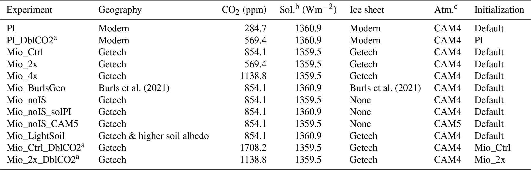
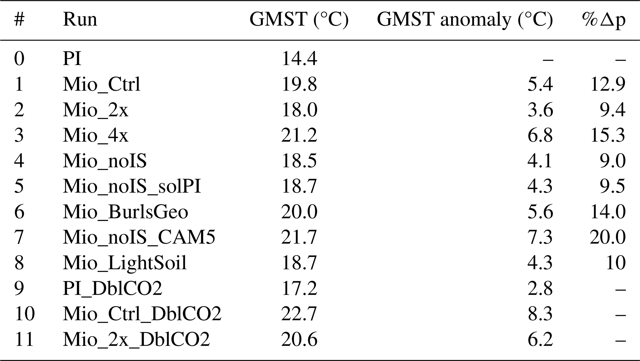
Burls et al. (2021)Burls et al. (2021)

Table 1 Summary of the experiments carried out in this study. “Getech” refers to the mid-Miocene geography provided by Getech Plc., whereas Burls et al. (2021) is a mid-Miocene geography. All runs have been integrated for at least 3100 years and up to 5000 years when using CAM5 (Mio_noIS_CAM5), unless specified with ^a where the simulations were ran for 150 years as to estimate ECS. ^b: Solar constant. ^c: Atmospheric model.

2 Methods

We use the Community Earth System Model version 1.2 (CESM1.2) to simulate mid-Miocene climate states. CESM1.2 is a coupled model using the ocean model POP2, with a 1° horizontal grid and 60 vertical levels and the CAM4 model for the atmosphere (Neale et al., 2013), applying a horizontal grid of 1.9×2.5° with 26 vertical layers, as well as a sea-ice model (CICE4), a river runoff model (RTM) and a land model which includes the carbon-nitrogen cycle and dynamical vegetation (CLM4). CESM1.2 has been used in numerous studies simulating different paleoclimates, such as the Last Glacial Maximum (LGM) (Kageyama et al., 2021; Zhu and Poulsen, 2021), the Pliocene (Haywood et al., 2020), the Eocene (Lunt et al., 2021) as well as older paleoclimates (Li et al., 2022).

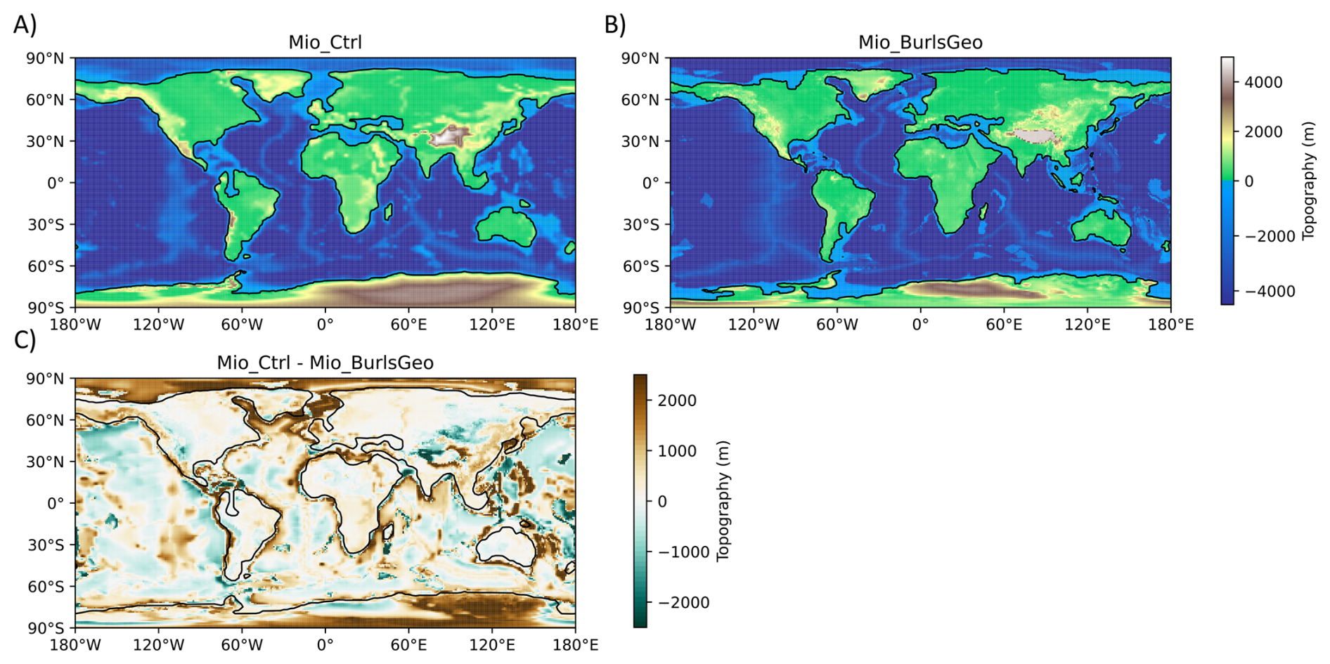
Figure 1 Topography and bathymetry for the two main paleogeographies in our simulations: (A) paleogeography of Mio_Ctrl, using Getech Plc. and (B) paleogeography of Mio_BurlsGeo based on Burls et al. (2021). (C) is the difference in topography between both paleogeographies. Except Mio_BurlsGeo, all simulations use (A) Getech Plc.

We perform a “best-to-knowledge” control simulation of the mid-Miocene (Mio_Ctrl), which includes an Antarctic ice sheet reconstruction, an updated CO₂ estimate, mid-Miocene solar constant, and is based on a topography and bathymetry reconstruction of the mid-Miocene, provided by Getech Plc. This reconstruction is based on geological data which include tectonics, sediment deposit and morphology, and which is fed into a tectonic model to generate paleogeographies at 0.1°×0.1° resolution, similarly as Lunt et al. (2016). The original geography as well as the plate model cannot be shared; however, the 1°×1° resolution used by CESM1.2 is shown in Fig. 1 and compared to an identical simulation using the paleogeography of MioMIP2 Phase 1 (Burls et al., 2021).

At the regional scale, the paleogeographies differ in both bathymetry and orography. The Getech paleogeography used in Mio_Ctrl features a notably shallower Arctic basin and generally higher elevations in mountainous and plateau regions compared to the Burls paleogeography. Due to lapse-rate effects, some of the surface temperature differences between the simulations likely arise directly from these topographic differences, particularly in regions such as the Rocky Mountains, the Andes, the Tibetan Plateau, and the Antarctic ice sheet. The Getech paleogeography also includes substantial changes in the representation of the South American Pebas mega-wetlands, which are absent in the Burls paleogeography. In addition, Greenland is represented as a slightly elevated plateau in Getech, rather than hosting an ice sheet. The Getech paleogeography differs from other recent mid-Miocene paleogeographies (e.g. Frigola et al., 2018; Scotese and Wright, 2018; He et al., 2021) primarily in the depths of the Fram Strait, the eastern and western seaways of the Tethys and the depth of the Panama seaway, which reflect uncertainties on the timing of closing, deepening or shoaling of these gateways during the Miocene in general. For instance, He et al. (2021) shows a much shallower eastern Tethys compared to Getech, and a western Paratethys connection, whereas Scotese and Wright (2018) displays a close eastern Tethys at the mid-Miocene. Both Frigola et al. (2018) and He et al. (2021) show a relatively shallow Panama seaway, which differ notably from Burls et al. (2021). Overall the Fram strait and earlier connections to the Arctic are much shallower in the geography of Getech than these other paleogeographies we are comparing to. To our knowledge, none of these geographies explicitly include the Pebas wetlands in South America. This may partly reflect differences in how wetlands are represented in climate models; in our case, the Pebas wetlands were treated as the shallowest level of the ocean model. Finally, paleogeographic reconstructions also differ in soil properties and vegetation type. In our simulations, vegetation type is simulated using a dynamic scheme.

The extent of Arctic and Antarctic ice sheets between Mio_Ctrl and Mio_BurlsGeo is compared to PI in Fig. 2. The ice sheets are considered as topographic objects and therefore the topography is flattened in Antarctica in the experiments where the ice sheets are not included. We then compare several Miocene simulations that differ in their solar constant (Mio_noIS_solPI), the presence of Antarctic ice sheet (Mio_noIS), and the atmospheric model used (Mio_noIS_CAM5), as to identify the role of each onto the mid-Miocene climate state. A summary of each experiment is given in Table 1.

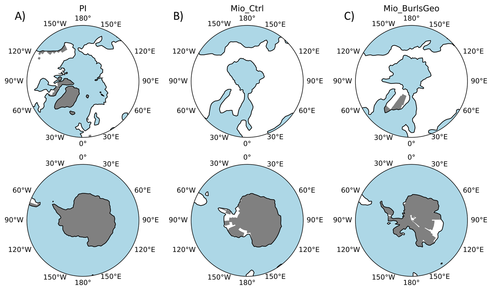
Figure 2 Land ice extent (filled contours) in the Arctic (top row) and the Antarctic (bottom row) regions in the three geographies used in this study: (A) PI, (B) Mio_Ctrl with the paleogeography of Getech and (C), Mio_BurlsGeo with the paleogeography of Burls et al. (2021). Note that the PI geography also includes high altitude glaciers, which are not all shown. Land masses are in white.

Unless specified for our sensitivity tests, our simulations use an atmospheric CO₂ concentration of 854.1 ppm, which is equivalent to three times PI CO₂ concentration of the model. This is planned as the standard concentration for the protocol of the MioMIP-phase 2 project. It is within the range of some reconstructions provided for the mid-Miocene (Rae et al., 2021; Steinthorsdottir et al., 2021), and it has also been used in other mid-Miocene simulations, which in general provides a closer match to proxy temperatures than simulations with lower CO₂ concentrations (Burls et al., 2021). The solar constant is calculated from a model of solar luminosity increase with time (Gough, 1981), which leads to a value of 1359.5 W m⁻² for the mid-Miocene, in comparison to 1360.9 W m⁻² at PI. Aerosols are kept as PI, but the sources are moved to match with the mid-Miocene paleogeography (for instance if an ocean turned to land). Non-CO₂ greenhouse gases and orbital forcing are kept as PI. Our simulations are compared to a proxy record presented in Burls et al. (2021). It is an agglomeration of sea-surface and surface temperatures based on multi-proxy reconstructions, where the sites are then rotated onto the mid-Miocene geography using the tectonic model of Getech Plc.

For estimating Miocene ECS in our simulation, we base our approach on a variation of Gregory et al. (2004), which would require an equilibrium simulation of the mid-Miocene with PI CO₂ concentration, from where a new simulation is initialized with an abrupt and sustained quadrupling of the CO₂ concentration, for around 150 years, so that “fast” climate feedbacks (i.e. clouds, surface albedo, water vapor, lapse-rate and Planck feedbacks) have mostly responded to the initial forcing. In the case of our simulations, a mid-Miocene state with PI CO₂ is numerically unstable, therefore we initialize from Mio_Ctrl by instead abruptly doubling its CO₂ concentration (Mio_Ctrl_DblCO2), as to avoid reaching excessively high CO₂ concentrations under a quadrupling, which could introduce non-linear effects on climate feedbacks. The ECS is then extrapolated from the global mean annual surface temperature after 150 years of simulation minus the initial temperature of the simulation using ordinary least squares linear regression. As to roughly estimate the influence of the Miocene background temperature on ECS, we also apply the same method but from a simulation at lower CO₂ concentration, Mio_2x (Mio_2x_DblCO2), and we compare it to a PI simulation with an abrupt doubling of CO₂ (PI_DblCO2).

The model is initialized from a warm ocean state, where the average deep-ocean temperature is around 6.6 °C. This value comes from an earlier, unpublished mid-Miocene simulation performed with CESM1.2, and is used to accelerate our deep-ocean equilibrium. The salinity is initialized globally at 35 PSU. In South America, in the so-called Lake Pebas, salinity becomes negative due to excessive precipitation and river runoff in these warm conditions. Therefore, we apply a marginal sea balancing scheme which redistributes the gain of freshwater onto the world oceans to avoid the spread of nonphysical, negative salinity into the oceans. This scheme has previously been used with CESM1.2 in warm paleoclimates (e.g. Lunt et al., 2021). The sea-ice model is initialized ice-free and the dynamic vegetation is initialized as bare soil. All runs have been integrated for at least 3100 years and up to 5000 years when using CAM5 (experiment Mio_noIS_CAM5), starting from default initial conditions, and the last 100 years are averaged and used for the results.

Several aspects of the ocean model are modified to handle the large changes in land-sea mask and bathymetry at the mid-Miocene. Overflows and tidal mixing are turned off, as they are hard-coded on a pre-industrial ocean grid. We follow the recommendations for deep-time paleoclimates of the National Center for Atmospheric Research (NCAR) to increase ocean background vertical diffusivity, to compensate for the lack of tidal mixing (found at https://www2.cesm.ucar.edu/models/paleo/faq/, last access: 11 April 2025). The same approach was taken by Baatsen et al. (2020) using CESM1.0.5 to simulate the Eocene. The background vertical diffusivity k_w is horizontally homogenous but depends on model depth, and corresponds to $k_w=\mathrm{vdc}\mathrm{1}+\mathrm{vdc}\mathrm{2}{\tan }^{-\mathrm{1}}\left(\right(\left|z\right|-\mathrm{depth}\left)\mathrm{linv}\right)$, where vdc1 =0.524 cm² s⁻¹, vdc2 =0.313 cm² s⁻¹, depth =1000 m, and linv $=\mathrm{4.5}\times {\mathrm{10}}^{\mathrm{-}\mathrm{3}}$ m⁻¹. This equation of background vertical diffusivity follows a Bryan and Lewis (1979) tangential profile, where the upper ocean diffusivity is 0.1 cm² s⁻¹ and the deep ocean diffusivity is a constant 1 cm² s⁻¹ below 1000 m. As a comparison, the PI state overall has a lower background diffusivity in the deep ocean, but the bottom-intensified tidal mixing can be up to two orders of magnitude larger than the background mixing. The timestep of the ocean model is reduced from calculating its step every 63 min model-time, to 41 min model-time. Modifying the timestep of models which use numerical integrations is known to affect their results, as was shown for CAM3 (Mishra and Sahany, 2011; Williamson, 2013), yet it remains generally poorly documented. It is not uncommon for paleoclimate simulations to use shorter computational time steps, as the ocean model in particular can generate numerous numerical instabilities which can lead to an early crash of the model. Our mid-Miocene results are compared to the “best-to-knowledge” PI simulation using modern parameterizations, as this should more accurately resemble the PI climate state. we explore the impact of these choice of ocean parametrizations in Appendix A, as further work on the ocean component of our mid-Miocene simulations is kept for a future study.

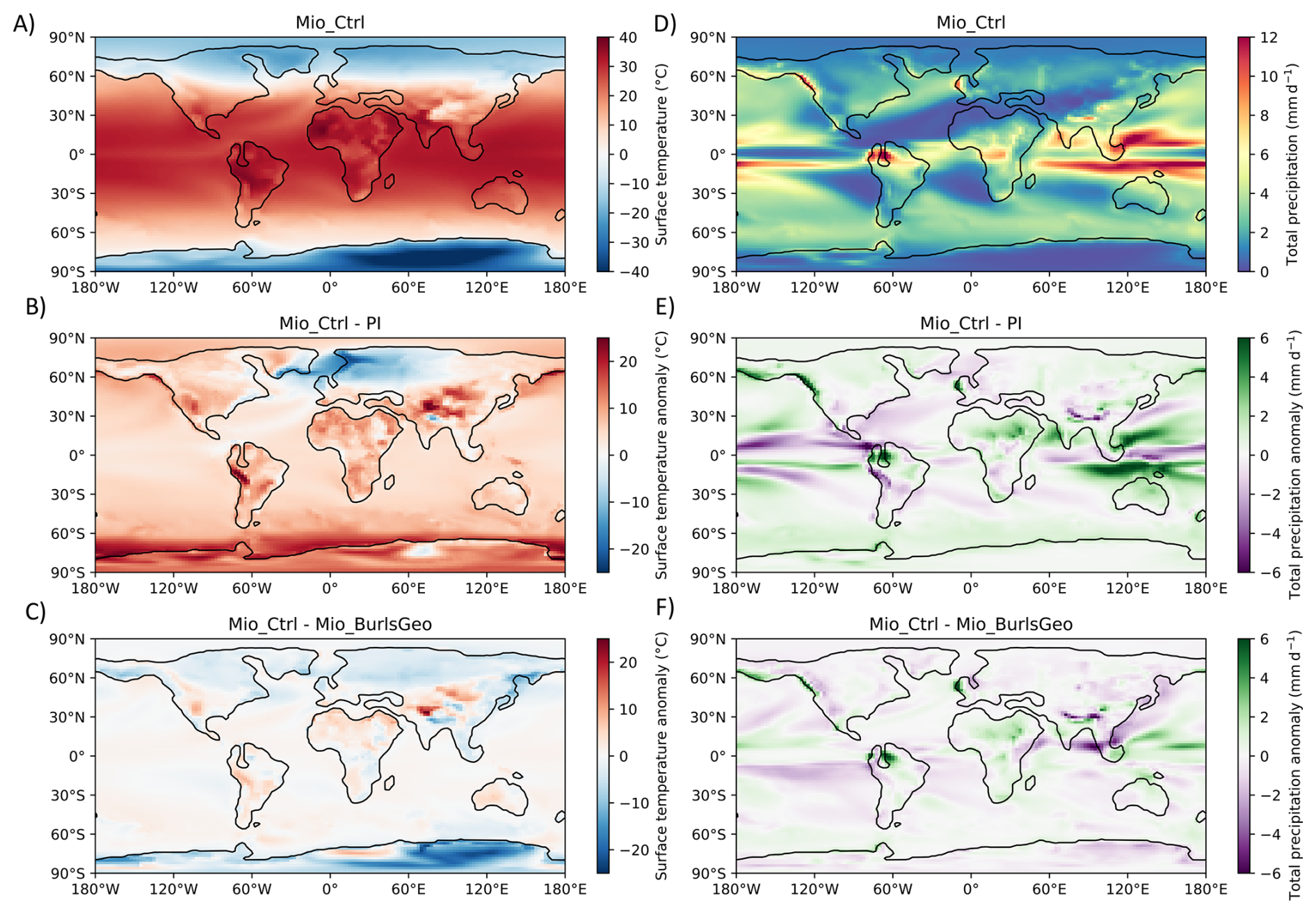
Figure 3 Surface temperature (A) and precipitation (D) maps of Mio_Ctrl, as well as comparison with PI (B, E) and with Mio_BurlsGeo (C, F).

3 Mid-Miocene control state

3.1 Climate

Our “best-to-knowledge” mid-Miocene simulation (Mio_Ctrl), which includes changes in paleogeography, ice sheet, CO₂ concentration, solar forcing and vegetation, is compared to PI and a similar mid-Miocene simulation using the paleogeography provided for MioMIP2 Phase 1 (Mio_BurlsGeo), in Fig. 3. Mio_Ctrl simulates a GMST of 19.8 °C, which is 5.4 °C warmer than PI (Table 2 and Fig. 3A). This temperature anomaly is in line with other simulations of the mid-Miocene Climate Optimum (MMCO) at lower CO₂ concentrations (Hossain et al., 2023; Wei et al., 2023; Sun et al., 2024), and is around 2 °C colder than the mid-Miocene simulations performed with HadCM3L at similar CO₂ concentrations (Burls et al., 2021).

Regionally, our mid-Miocene simulations (Mio_Ctrl and Mio_BurlsGeo) both show a substantial warming over the southern high latitudes (Fig. 3B), linked to polar amplification, and a large cooling pattern over the north Atlantic ocean and northern Europe. The latter is likely connected to an absent Atlantic Meridional Overturning Circulation (AMOC), which is replaced by a Pacific Meridional Overturning Circulation (PMOC). The absent AMOC implies a reduced northward heat transport in the North Atlantic and towards the Arctic ocean. The Arctic, in turn, is shallow and has limited exchanges with the Atlantic ocean in these paleogeographies. This likely contributes to the apparent absence of polar amplification in the northern hemisphere temperature signal. An absent AMOC in favor of the PMOC has been seen in other mid-Miocene simulations but remains a rare phenomenon within MioMIP, and is not supported by proxy data (Hutchinson et al., 2025; Naik et al., 2025). Although this result is relevant for future climate change and for understanding the conditions under which a PMOC state can be sustained, it will be addressed in a separate paper focusing on the ocean component of our simulations.

Comparing both paleogeographies, Mio_BurlsGeo is slightly warmer than Mio_Ctrl by 0.2 °C (Table 2 and Fig. 3C). Mio_BurlsGeo was initialized with a slightly lighter color of soil, equivalent to a dry albedo increase of around 0.1 and a saturated soil albedo increase of around 0.05 compared to the darker soil of Mio_Ctrl and other simulations using the Getech paleogeography. Soil properties are rarely documented in past modelling studies, mainly due to the fact that there is limited information on soil albedo in geological times. However, testing the effect of soil properties can be relevant in future paleomodelling efforts, in particular as it interacts with dynamic vegetation. Adjusting the soil color of Mio_Ctrl to that of Mio_BurlsGeo in a simulation called Mio_LightSoil leads to a GMST of around 18.7 °C, and so a difference with Mio_BurlsGeo of around 1.3 °C. While there is limited constraint on soil properties in paleo settings, and it is largely dependent of i.e. soil type, humidity, vegetation cover, ice sheet, we emphasize that documenting these properties is relevant as they may partially contribute to the mid-Miocene climatic patterns.

Mio_BurlsGeo was also initialized with PI solar forcing as to provide a better comparison with previously published mid-Miocene runs. As discussed in Sect. 6.3, a simulation with PI solar forcing (Mio_noIS_solPI) shows an additional warming of around 1 °C in high latitudes. However, as also discussed in Sect. 6.3, the difference of solar constant between Mio_BurlsGeo and Mio_Ctrl is mostly negligible compared to the other forcing discussed in this study.

Similarly as for temperature, we analyse total precipitation in Mio_Ctrl (Fig. 3D) with respect to PI and Mio_BurlsGeo. Globally, Mio_Ctrl is 12.9 % wetter than PI (Table 2 and Fig. 3E) and is wetter than mid-Miocene simulations using HadCM3L at 850 ppm of CO₂ (around 10 %, Acosta et al., 2024). Mio_Ctrl is characterized by drier conditions in the eastern Pacific and wetter conditions in the western Pacific, as well as a common double Intertropical Convergence Zone (ITCZ) bias over the basin (Song and Zhang, 2019). This is in good agreement with the multi-model mean of mid- to late Miocene simulations at 560 ppm of CO₂ (Acosta et al., 2024). The north Atlantic region is drier than PI, and similar results are obtained from HadCM3L and CCSM4 simulations (Burls et al., 2021; Acosta et al., 2024).

Mio_BurlsGeo is slightly wetter than Mio_Ctrl (Fig. 3F), and 14 % wetter than PI (Table 2). Precipitation patterns are partly affected by the differences in coastlines and topography as seen in Fig. 1. In the tropics, the absence of the Pebas wetlands in Mio_BurlsGeo results in drier conditions in the northern part of South America. In contrast, the South-East Pacific, North-East Asia and South-East Asia regions are wetter and the latter is, in fact, the largest precipitation change between both geographies. The main characteristic of this region is an enhanced connection between the Pacific and the Indian oceans which is not present in Mio_Ctrl.

Table 2 Summary of global mean surface temperature (GMST) and the anomaly relative to the PI simulation, and percent change of total precipitation (%Δp) relative to PI in our simulations.

3.2 Vegetation

Biomes based on vegetation distribution are challenging to reconstruct in deep time paleoclimates, notably due to the difficulties in preserving land proxy data and because the plant pollen can be deposited far from their sources. However, vegetation plays an important role in past climates as it provides feedbacks on moisture and temperature changes, and can be used to reconstruct atmospheric CO₂ concentrations. The mid-Miocene is particularly relevant as it displays the largest flora change of the Cenozoic and the emergence of modern biomes (Steinthorsdottir et al., 2021).

Coupled climate-vegetation models have been used in past climate simulations (e.g. Stepanek et al., 2020), with relatively good agreement with proxy data, albeit large local differences can be seen. Here, we show the simulated vegetation for Mio_Ctrl (Fig. 4) and compare it to the reconstructed biomes for the mid-Miocene of Steinthorsdottir et al. (2021).

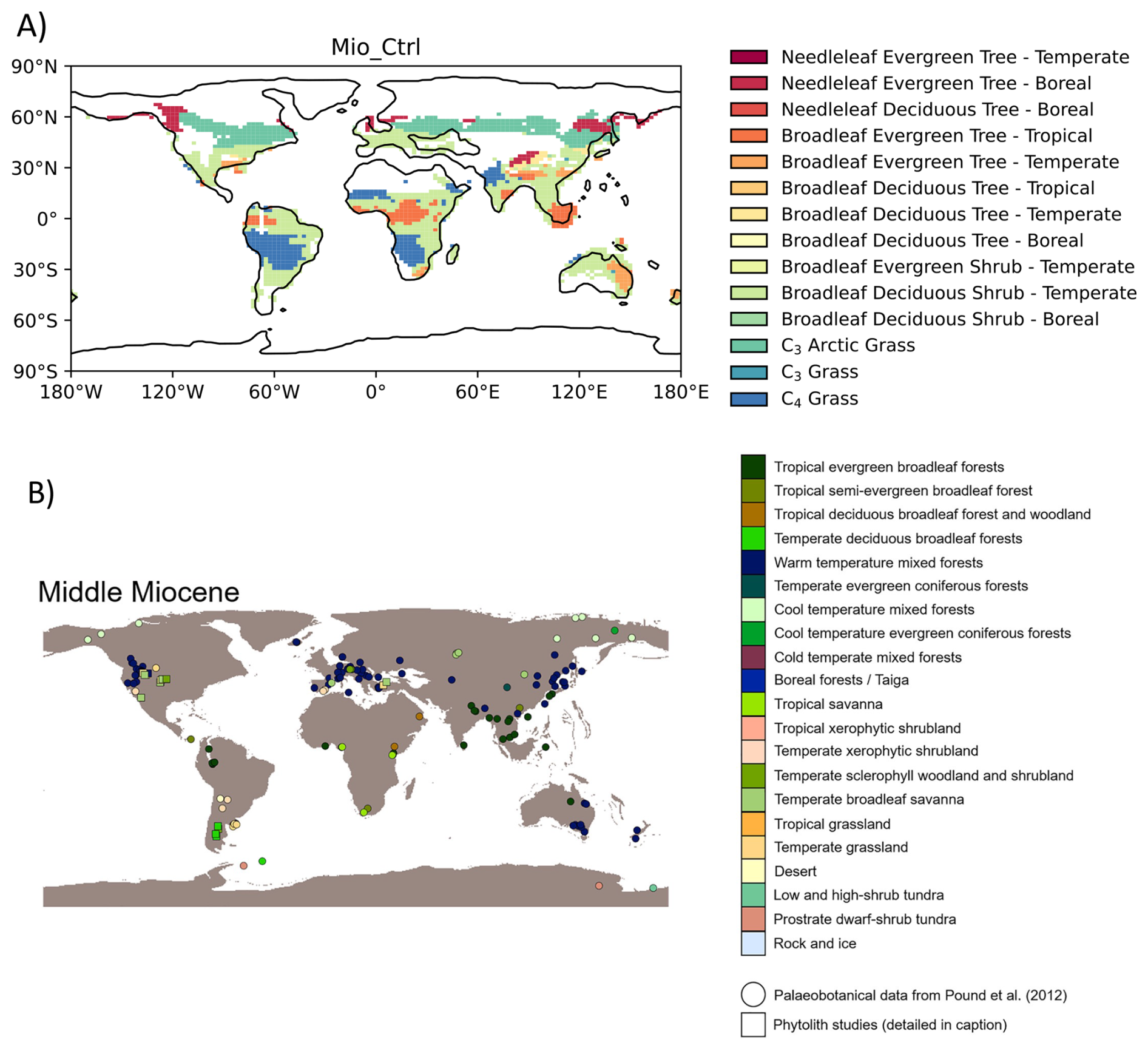
Figure 4 (A) Simulated vegetation types in Mio_Ctrl compared to (B) reconstructed biomes for the mid-Miocene, adapted from Steinthorsdottir et al. (2021). In (A), the soil is bare if the sum of the contribution of all vegetated areas is less than 10 %.

The proxy record indicates a large spread of temperate forests and savanna in mid-latitudes during the mid-Miocene, notably in Europe, north-east Asia and Australia. Although our vegetation model also simulates temperate biomes for Europe and Australia, predominantly composed of temperate shrubs or evergreen temperate forests, we observe Arctic (dominated by Arctic grass) and boreal (dominated by boreal evergreen trees) climates in North East Asia and northern Europe, and almost no vegetation growth above 60° N. On the contrary, the proxy record still indicates (cool) temperate forests, even at latitudes higher than 60° N.

Overall, our predicted vegetation mirrors our model-data temperature map: there is a good agreement in tropical regions between model and proxy data, but our simulated biomes are contracted towards the Equator, with warmer types of vegetation constrained in the lower latitudes and therefore fail to match mid to high latitude biomes as seen in the proxy record. This is likely both a result of and feedback on temperature, as vegetation usually has a lower albedo than bare soil.

4 Impact of CO₂

There have been different plausible estimates of atmospheric CO₂ concentrations for the mid-Miocene due to differences in methodology and calibrations (Burls et al., 2021). The concentration is usually thought to lie between two and three times PI concentrations, three being the concentration discussed for the upcoming MioMIP experimental design, in line with recent high estimates during the MMCO (around 700–1100 ppm, Rae et al., 2021). Here, we compare Mio_Ctrl, which has a CO₂ concentration of three times PI, to two simulations using mid-Miocene boundary conditions and two times (Mio_2x) and four times (Mio_4x) PI in Fig. 5, relative to the proxy record. Although CO₂ concentrations as high as four times PI during the mid-Miocene are at the high threshold of the estimates, such levels are useful for estimating ECS and feedbacks (Farnsworth et al., 2019), which are both important elements for quantifying global and regional responses to CO₂.

In Mio_2x, the GMST is 18.0 °C, which is 3.6 °C warmer than PI (Table 2), and even lower than proxy estimates of the colder Late Miocene (Burls et al., 2021). In Mio_4x, the GMST is 21.2 °C, and its anomaly relative to PI is 6.8 °C (Table 2). This is in agreement with proxy estimates for the GMST of the mid-Miocene. Similarly, Acosta et al. (2024) showed that CO₂ concentrations between three and four times PI concentrations provide the most reduced bias in total precipitation at a global scale, but some regions critically lack proxy sites, and there are few simulations at such high CO₂ concentrations for comparison (Burls et al., 2021).

At all CO₂ levels, the mid-Miocene simulations are cold and underestimate surface temperatures reconstructed from proxy data in most mid to high latitudes locations (Fig. 5). The cold pattern simulated in the north Atlantic contributes even more to the temperature bias relative to proxy data. This pattern is likely connected to an absent AMOC in our model at all three CO₂ levels. Problematically, a weak mid-Miocene AMOC is a persistent feature in climate models (Naik et al., 2025), with some rare exceptions (Tan et al., 2026), the associated colder North Atlantic surface temperature is not necessarily supported by proxies (e.g. Sepulchre et al., 2014). Nevertheless, a recent study using coccolith clumped isotopes showed a modest northern Atlantic warming during the mid-Miocene compared to the high warming reported in earlier studies (Mejía et al., 2025), which suggest that some model-proxy discrepancies may be due to limitations in proxy interpretation. Further discussion on the ocean circulation in our simulations is planned for a follow-up paper.

In Mio_2x, the temperatures are too cold even in tropical locations compared to proxy data (Fig. 5). On the contrary, in Mio_4x, some of the mid and high latitudes negative biases are dampened, but tropical locations are too warm compared to proxy data. These issues affecting polar and tropical warmth are commonly found in other Miocene simulations with various models (Burls et al., 2021), and most mid-Pliocene simulations during PlioMIP1 (Haywood et al., 2011), although there was no systematic bias in PlioMIP2 models (Haywood et al., 2020). Climate models are not tuned for paleoclimates, which contributes to the challenges they face in representing polar amplified temperatures in warm paleoclimates (Burls and Sagoo, 2022). Moreover, climate models may show other biases in high latitudes, notably due to poor representation of vegetation from dynamic vegetation models, as shown in Sect. 3.2, or lack of interactive ice sheets. Additionally, it is likely that model-proxy biases are a combination of both model and proxy errors. Notably, pollen and marine organic proxies can have substantial seasonal biases, which can strongly affect their temperature signal when compared to annually-averaged modelled temperatures, as described by Tindall et al. (2022) for the Pliocene.

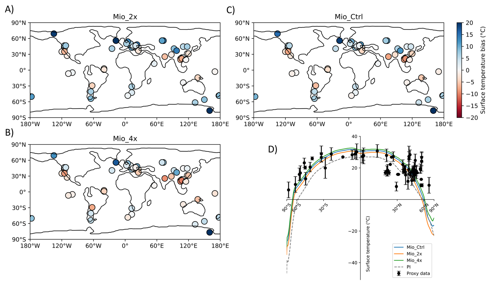
Figure 5 Surface temperature biases relative to the proxy record at (A) 2 (Mio_2x), (B) 4 (Mio_4x) and (C) 3 (Mio_Ctrl) times PI CO₂ concentrations, at proxy sites and (D) zonally. Proxy sites are rotated on the mid-Miocene geography with the tectonic model of Getech Plc.

5 Equilibrium Climate Sensitivity

ECS is widely regarded as one of the most critical metrics for characterizing future climate change (Forster et al., 2021; Huusko et al., 2021). However, due to the difficulty of constraining it, several independent methods have been used, notably including evidence from the paleoclimate record (e.g. Crucifix, 2006; Hargreaves et al., 2012; Rohling et al., 2012; Renoult et al., 2020; Sherwood et al., 2020). Some of these methods involve directly calculating the radiative forcing and global temperature of a past climate from the proxy record (e.g Rohling et al., 2012; Sherwood et al., 2020; Tierney et al., 2020), or emergent-constraint approaches, which are statistical methods connecting proxy reconstruction with the outputs from several models, usually under the umbrella of a MIP, such as for the LGM under PMIP (Hargreaves et al., 2012; Renoult et al., 2020, 2023) or PlioMIP (Hargreaves and Annan, 2016; Haywood et al., 2020; Renoult et al., 2023).

The ECS of a paleoclimate and how it relates to modern ECS is not necessarily obvious. The effects of “fast” climate feedbacks (i.e. clouds, surface albedo, water vapor, lapse-rate and Planck feedbacks) need to be disentangled from “slow” climate feedbacks (notably carbon cycle, ice sheets and aerosols feedbacks), where the latter affects temperature on geological time-scale and usually connect to a different concept, the Earth system sensitivity (Rohling et al., 2012; Lunt et al., 2010). Climate feedbacks also depend on the background climate and the forcing imposed, which can lead to high ECS in warm, high-CO₂ paleoclimates (Caballero and Huber, 2013; Anagnostou et al., 2020). Those aspects result in important challenges when using evidence from new paleo-MIP to deduce ECS (Rohling et al., 2012; Renoult et al., 2023).

A way to approach these issues is to estimate ECS directly from a paleoclimate simulation, and compare it to the ECS in a modern simulation in the same model (e.g. Farnsworth et al., 2019). Here, we have performed two simulations: Mio_Ctrl_DblCO2, which corresponds to a doubling of CO₂ from Mio_Ctrl (1708.2 ppm), and Mio_2x_DblCO2, which is a doubling of CO₂ from Mio_2x (1138.8 ppm). Further details on the methodology are provided in Sect. 2.

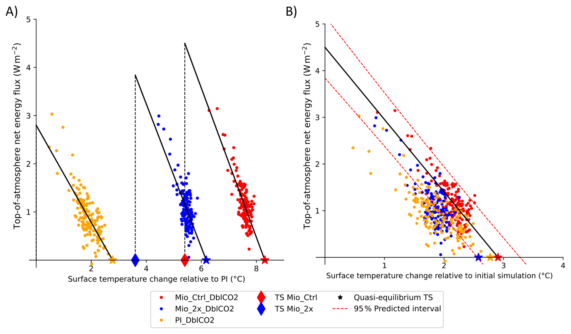
Figure 6 Top-of-atmosphere energy flux (W m⁻² versus global mean surface temperature where (A) the simulations temperature are reported relative to the PI temperature and (B) the simulation temperatures are reported relative to their initial state (PI or mid-Miocene). The stars (one for each simulation/color) are estimates of the long-term near-equilibrium temperatures using ordinary least squares linear regression.

In Mio_Ctrl_DblCO2 (1708.2 ppm), ECS is 2.9 °C (2.5–3.3 °C, 95 % predicted interval, Fig. 6B), in comparison to 2.8 °C from PI conditions with this model (2.2–3.4 °C, 95 % predicted interval, Fig. 6A). From a lower CO₂ concentration, Mio_2x_DblCO2 (1138.8 ppm), ECS is 2.6 °C, which, similarly as the estimate from PI climate, is also within the 95 % predicted interval for the ECS of Mio_Ctrl_DblCO2. Even when considering the higher background CO₂ concentration, and consequently higher background mean temperature of the mid-Miocene, these estimates tend to indicate that the PI-based ECS of CESM1.2 can characterize the Miocene climate, or that ECS estimates obtained from the Miocene climate using CESM1.2, for instance in an emergent constraint approach, could be representative of its modern-based ECS. Previous studies on the Miocene have also estimated its ECS to be close to 3 °C, and in general relatively close to the ECS estimated for modern climate from Miocene evidence (Tong et al., 2009; Rohling et al., 2012; Bradshaw et al., 2015; Brown et al., 2022), as well as the ECS reported from multiple lines of evidence in the latest assessment report of the International Panel on Climate Change (IPCC AR6: 3 °C, 2–5 °C, 90 % confidence interval, Forster et al., 2021), in comparison to some older warm paleoclimates (e.g. the Eocene) where ECS estimates easily exceed 6 °C (Anagnostou et al., 2020).

6 Additional sensitivity studies

Here, we investigate the impact of the Antarctic ice sheet, atmospheric model, and solar constant on the mid-Miocene temperature and precipitation. The sensitivity runs for the atmospheric model and the solar constant were performed without the Antarctic ice sheet, as the ice sheet data was not available to us at the time of the simulations, and these simulations are computationally expensive to perform. Therefore, in this section we use Mio_noIS, a mid-Miocene simulation without Antarctic ice sheet as the control simulation around which the sensitivities are tested. Global temperature anomalies and percent change of total precipitation relative to PI are reported in Table 2.

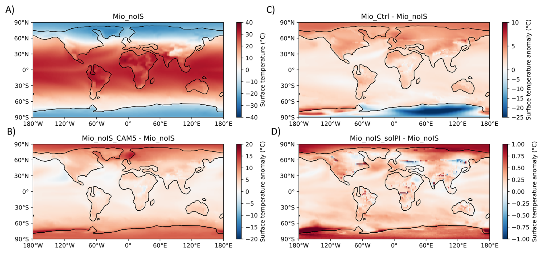
Figure 7 Surface temperature maps for the different sensitivity experiments, using the no-ice-sheet (Mio_noIS, panel A) experiment as a control state: (B) anomaly from Mio_noIS_CAM5, (C) anomaly from Mio_Ctrl and (D) anonaly from Mio_noIS_solPI. Note the differences in scale.

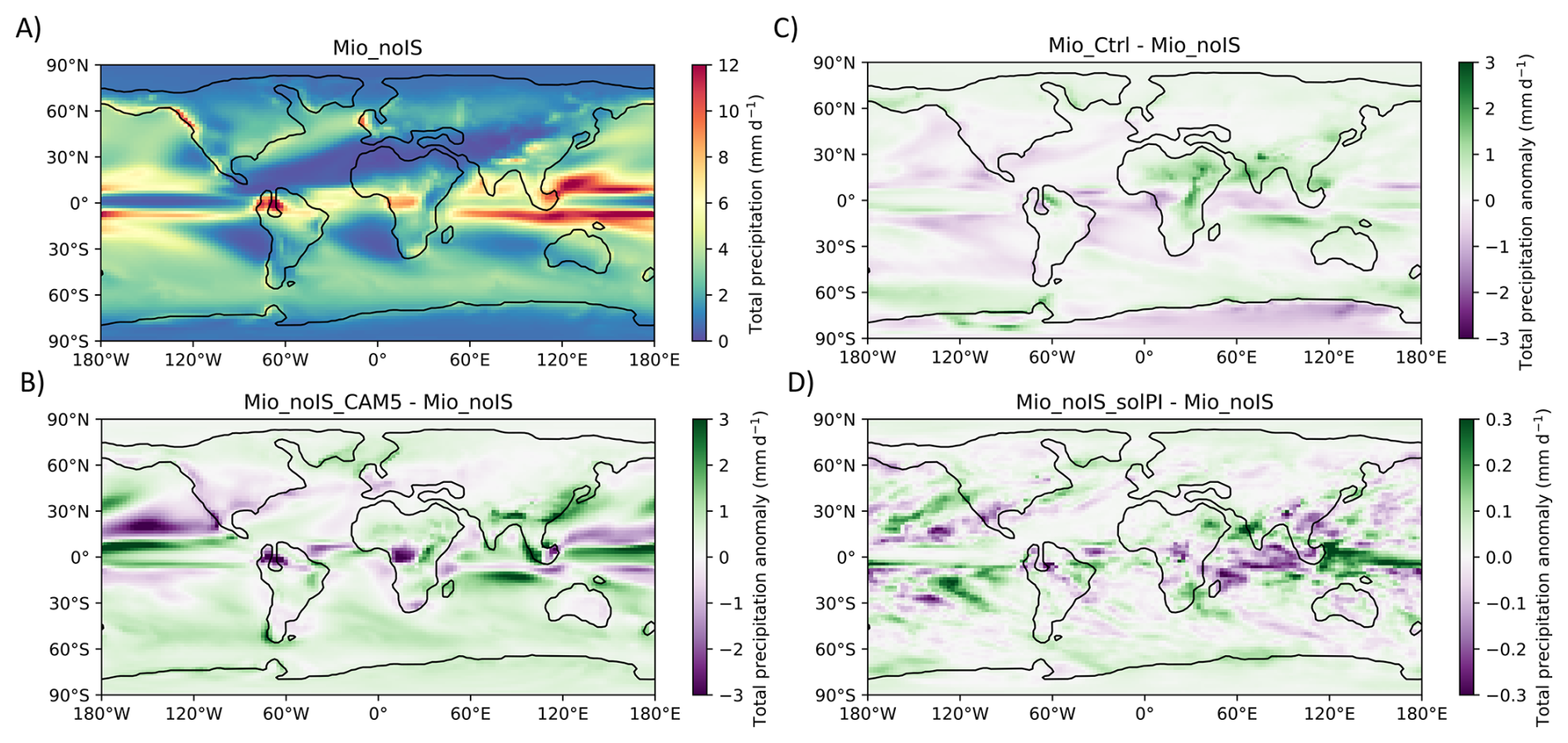
Figure 8 Total precipitation maps for the different sensitivity experiments, using the no-ice-sheet (Mio_noIS, panel A) experiment as a control state: (B) anomaly from Mio_noIS_CAM5, (C) anomaly from Mio_Ctrl and (D) anonaly from Mio_noIS_solPI. Note the differences in scale.

6.1 Impact of atmospheric model

Model parametrizations play an important role on climate. In the Pliocene Modelling Intercomparison Project Phase 2 (PlioMIP2), three versions of CCSM4 simulated the mid-Pliocene (CCSM4-Utrecht, CCSM4-NCAR and CCSM4-UoT). The global mean surface temperature difference between the warmest CCSM4 (CCSM4-Utrecht) and the coldest CCSM4 (CCSM4-UoT) was as large as the global mean surface temperature difference between the coldest CCSM4 version and PI climate (Haywood et al., 2020). CCSM4 is a model of the CESM model family (notably containing CCSM3, CCSM4, CESM1.2, CESM1.3, CESM2, i.e. built on similar versions of submodel components developped at NCAR), such as CESM1.2 which we are using for our mid-Miocene simulations. Throughout the model family history, there have been substantial changes in parametrizations, with the most recent CESM2 having one of the largest ECS of modern climate model ensembles (Gettelman et al., 2019).

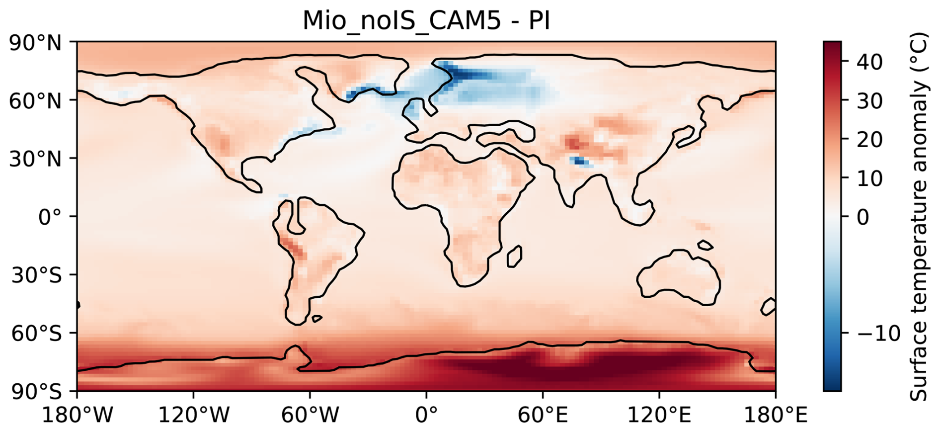
Figure 9 Map of surface temperature differences between Mio_noIS_CAM5 and PI. Note that the color mapping is non-linear.

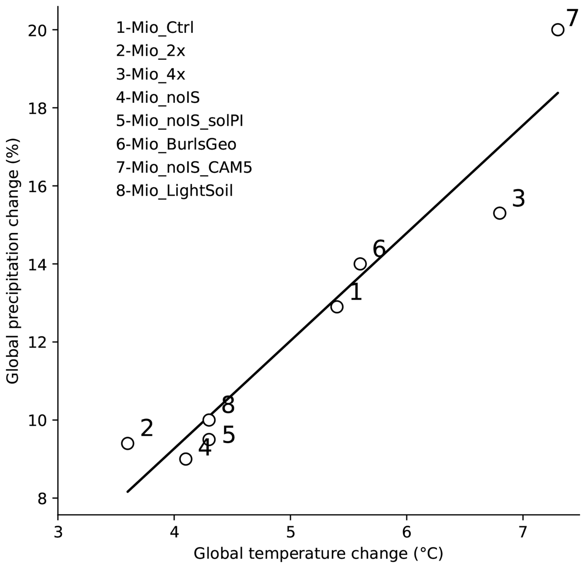
Figure 10 Global temperature change (°C) versus global precipitation change (%) relative to PI across all our mid-Miocene simulations (as numbered in Table 2) initialized from default model conditions.

Similarly as for temperature, changing the atmospheric model from CAM4 to CAM5 has a considerable effect on precipitation. Globally, we observe an increase to total precipitation of 20.0 % relative to PI, which is also 11 % larger than Mio_noIS (Table 2). Overall, there is a tight coupling between the global mean temperatures and global precipitation changes across our different simulations and independently of the choice of atmospheric model, as shown in Fig. 10. This is to be expected from the Clausius-Clapeyron relation, and it is an indicator of the dominant role of global temperature change on global precipitation, whereas the different sensitivities tested in this study (e.g. topography, atmospheric model), are more likely to affect regional precipitation. For instance, as earlier mentioned, CAM5 saw substantial changes in mid to high latitudes cloud parametrizations and microphysics scheme relative to CAM4, where we observe much wetter conditions in those regions with CAM5 in our simulations (Fig. 8), particulary in the Southern hemisphere and the northern Pacific ocean. This is at first not expected because CAM5 saw reduced non-convective precipitation relative to CAM4 (Chen and Dai, 2019), so the increase in high latitude precipitation is more likely a response of CAM5 to CO₂ rather than differences in parametrizations between both atmospheric models. On the contrary, CAM5 displays enhanced convective precipitation relative to CAM4 (Chen and Dai, 2019), and over the equatorial Pacific ocean, a wetter double ITCZ band is observed in future scenarios using CAM5 compared to CAM4 (Meehl et al., 2013), which could contribute to the substantial wettening of the equatorial Pacific ocean in Mio_noIS_CAM5. Drier conditions are observed over North America and in the eastern subtropical Pacific ocean. Contrarily to simulations using CAM4, the Pebas wetlands has a less pronounced impact on South American precipitation.

An issue in paleo MIPs is that they often include several versions of the same models with apparent small differences between them due to the cost and technical difficulties which surround paleoclimate modelling. This was the case with three versions of CCSM4 at PlioMIP2 (Haywood et al., 2020) or multiple versions of CCSM3 and HadCM3L for MioMIP (Burls et al., 2021). This can impact multi-model comparisons as well as model-proxy comparisons, as similar biases are replicated and have a bigger weight on the ensemble. Here, we have shown that moving from CAM4 onto CAM5 leads to a substantial difference in mid-Miocene climate. Thus, small changes of parametrizations between relatively similar models can generate a large array of responses and can easily justify the presence of these models together within a MIP.

6.2 Impact of Antarctic ice sheet

Geological evidences show a substantial retreat of the Antarctic ice sheet during the early to mid-Miocene, in particular during the MMCO (Gasson et al., 2016). In the two paleogeographies used in this study, we report a reduction in Southern hemisphere land ice area (which also include Andean glaciers) of 18 % using the paleogeography of Getech, and 31 % using the paleogeography of Burls et al. (2021) relative to our PI state. For the Northern hemisphere, there is no land ice in the Getech paleogeography, and a reduction of 80 % using the paleogeography of Burls et al. (2021). The extent of the land ice is shown in Fig. 2.

Through modification of the surface albedo, the topography and the atmospheric and ocean circulations, ice sheets have a substantial impact on the climate (Gasson et al., 2016). Here, we test the impact of the Antarctic ice sheet on the mid-Miocene climate by comparing to Mio_Ctrl a simulation where we removed the ice sheet and jointly flatten the Antarctic continent (Mio_noIS). Although there is a net reduction in the land ice area in our mid-Miocene simulations compared to PI, we would still expect the presence of ice sheets in Mio_Ctrl to cool down the climate relatively to Mio_noIS, notably through the increase of surface albedo. Instead, implementing the Antarctic ice sheet in Mio_Ctrl warms up the global climate by 1.4 °C and makes it 3.9 % wetter compared to Mio_noIS (Table 2).

When comparing both cases with and without ice sheet in Fig. 7, we observe that the presence of the ice sheet locally cools down Antarctica by around 25 °C at its highest altitude. However, there is also a substantial warming in the Arctic ocean and over the northern hemisphere continental masses, as well as a smaller warming over the global ocean. Mio_noIS shows almost no warming at all in the Arctic region relative to PI, which differs from Mio_Ctrl. Over the oceans, mid and low latitude regions are drier or wetter in Mio_Ctrl if they are respectively dry and wet in Mio_noIS. High latitudes tend to be wetter in Mio_Ctrl, except directly over the Antarctic ice sheet. A substantial wettening of Eastern Africa can be observed in Mio_Ctrl, as well as Southern Asia.

Atmospheric and oceanic heat transport are similar between the simulations, indicating that the higher Northern Hemisphere temperatures are not due to enhanced heat transport from the south (Appendix B). Instead, the radiation budget in the northern high latitudes suggests that the warming could be a result of a complex interplay between cloud and ice fraction forces and feedbacks. A detailed investigation of these mechanisms is beyond the scope of this study, but we briefly discussed it in Appendix B, as it could highlight some processes which affect polar amplification in warm paleo-simulations.

6.3 Impact of solar constant

Of all the forcing applied to our mid-Miocene simulations, the change from PI solar constant to mid-Miocene solar constant has the least impact. Mio_noIS_solPI is around 0.2 °C warmer than Mio_noIS (Table 2) globally, whereas most of the warming comes from high latitudes where the temperatures are 1 °C warmer (Fig. 7). The small amplitude of this change is expected, as the mid-Miocene solar constant is estimated to be 0.1 % less than PI solar constant (Gough, 1981). As a comparison, a doubling of atmospheric CO₂ (around 3.7 W m⁻², Myhre et al., 1998) is roughly equivalent in forcing to an increase of 2.25 % of solar constant, assuming a planetary albedo of 0.7. Therefore, the change of solar constant is mostly negligible, but could be partially responsible for the high latitudes of Mio_BurlsGeo being warmer than Mio_Ctrl which uses a mid-Miocene solar constant.

7 Conclusions

In this study, we have developed a set of simulations using a new and previously unpublished geography for the mid-Miocene, using CESM1.2. Research centered on the mid-Miocene has shown a potential for it to be a partial analog of near-future climate (e.g. Steinthorsdottir et al., 2021), yet uncertainties remain on atmospheric CO₂ concentration and non-CO₂ forcing, and consequently the scale of the warming and the strength of its potential analogy. In particular, model simulations do not match the high latitude warming inferred from some proxies, potentially due to changes in ocean circulation, poor understanding of polar amplification in models or poor representation of vegetation. Alternatively, proxy-reconstructed temperatures might also be uncertain, as recent studies suggest colder mid-Miocene northern Atlantic temperatures, more in-line with climate models' outputs (Mejía et al., 2025). It is in fact likely that these discrepancies reflect issues from both models and proxies, and the mid-Miocene experiments performed in this study aimed to bring a new light onto those questions.

Variations in CO₂ concentrations for the mid-Miocene have a substantial influence on its estimated temperatures. Between the high end (four times PI concentration) and the low end (two times PI concentration) of tested concentrations, we find a difference of 3.2 °C on mid-Miocene global mean surface temperature, suggesting a substantial role of CO₂ forcing on the mid-Miocene climate, as also previously observed in the case of the Pliocene (Burton et al., 2023). The mid-Miocene is also sensitive to non-CO₂ forcing, such as the land-sea mask, ice sheet and solar forcing, but the variations tested for those components had a lower influence on the mid-Miocene temperature than CO₂. Finally, we identified that switching the atmospheric model from CAM4 to CAM5, which has a substantial influence on cloud feedbacks, leads to a warmer mid-Miocene by up to 3.2 °C, which highlights the critical need of improving model climate feedbacks, as much as it is to better constrain climate forcing in paleoclimates.

Similarly as for the LGM (Hargreaves et al., 2012; Renoult et al., 2020) and the Pliocene (Hargreaves and Annan, 2016; Haywood et al., 2020; Renoult et al., 2020), the mid-Miocene can be used to quantify ECS, owing to its relative proximity to modern climate. In this study, we estimated that the ECS of CESM1.2 at the mid-Miocene is 2.9 °C (2.5–3.3 °C, 95 % prediction interval), which is close to the modern-based estimate of ECS of CESM1.2 (2.8 °C, 2.2–3.4 °C, 95 % prediction interval). From this short glance on ECS in CESM1.2, as well as previous work on Miocene ECS (Tong et al., 2009; Rohling et al., 2012; Bradshaw et al., 2015; Brown et al., 2022), we believe there is motivation in supporting ECS estimates using Miocene evidence, particularly as Miocene modelling is moving towards an official PMIP design. Despite uncertainties in the proxy record or model disagreements, the Pliocene, the warm epoch following the Miocene, has shown that recent warm paleoclimates can provide robust constraint on ECS (Hargreaves and Annan, 2016; Haywood et al., 2020; Renoult et al., 2023). Additionally, emergent constraint framework can be used to identify disagreements between models, and between model and data (Renoult et al., 2023). Thus, estimates from the Miocene could either support existing methods using paleoclimate evidence (Sherwood et al., 2020; Cooper et al., 2024), or be used within a new emergent constraint framework as previously done with emergent constraint frameworks for the LGM (Hargreaves et al., 2012; Renoult et al., 2020) or the Pliocene (Hargreaves and Annan, 2016; Haywood et al., 2020; Renoult et al., 2023).

Compared to the proxy record, mid-Miocene simulations are usually either too cold globally, too cold at high latitudes, or both (Burls et al., 2021). Over different sensitivity experiments, we find the same issues using CESM1.2, which arise from a weak polar amplification. Simulated high latitudes temperatures underestimate the proxy record by as much as 20 °C, and warm vegetation biomes are more contracted towards low latitudes. However, high CO₂ levels and better representation of high latitude cloud parametrizations produce a better match with high latitude proxy sites and also provided a better match with precipitation proxy reconstruction (Acosta et al., 2024). Additionally, northern Atlantic sea-surface temperatures reconstructed from coccolith clumped isotopes suggest a more modest warming compared to PI (Mejía et al., 2025). This would lead to a decrease in the proxy-model bias observed in this region, without overestimating low-latitude ocean temperatures, as inferred from high-CO₂ simulations.

A mid-Miocene state close to reality is likely to include a combination of different sensitivities tested in this paper. A continued focus on high-latitude climate feedbacks to enhance polar amplification in models remains important, as this has been a recurring challenge in paleoclimate simulations and could influence projections of future climates. Further research is also needed to assess potential biases and uneven coverage in the proxy record, which can still affect model-proxy comparisons and interpretations of global Miocene climate.

Appendix A: Ocean model timestep and parametrizations

Although changes in ocean parameterization are often required for the numerical stability of paleoclimate simulations, their potential consequences on the climate remain rarely documented. Here, we investigate whether the changes we imposed on our simulations impact our results. These changes are described in Sect. 2 and are namely turning off overflows and tidal mixing, adding a background vertical diffusivity and reducing the timestep of the ocean model.

Because these changes are necessary for the stability of our paleoclimate simulations, in particular aspects such as overflows which are hard-coded onto PI geography, we cannot test their impacts onto the mid-Miocene runs. Instead, we apply these configurations to two PI simulations: one, named PI_OcnTimStp, where only the timestep for the computation of the ocean model is reduced from a 63 min timestep to a 41 min timestep; one, named PI_OcnParam, where the full list of changes is applied, including turning off overflows, tidal mixing, adding the background vertical diffusivity coefficient and reducing the ocean timestep. Figure A1 summarizes the differences in surface temperatures and AMOC strength relative to the original PI simulation used in our study. We observe colder temperatures by up to 10 °C in localized areas in the North Atlantic ocean where deep-water formation occurs, and a more broad cooling over the Arctic ocean of around 2 °C, as well as a warming of the Southern Ocean by around 1.5 °C in PI_OcnParam relative to PI (Fig. A1A). The temperature differences between PI_OcnTimStp and PI are more negligible (Fig. A1B). The maximum AMOC strength compared to PI (Fig. A1C) weakens by up to 2 Sv in PI_OcnTimStp (Fig. A1D), and by 2.6 Sv in PI_OcnTimStp (Fig. A1E).

We highlight that these results are difficult to convey for the mid-Miocene simulations. The changes in ocean parametrizations target specific PI locations which are hard-coded for its geography, but also locations that are connected to stronger circulation. Therefore, we cannot conclude on the impact of the ocean parametrizations on mid-Miocene simulations, because: (1) they have an ocean model initialized uniformly, without any circulation, and (2) they show a PMOC, whereas the colder temperatures found in PI_OcnParam might be a feedback from the weakened AMOC, and the warmer temperatures in the Southern Ocean due to seesaw effect also from the weaker AMOC.

One could hypothesize that the ocean parametrizations imposed on CESM1.2 is responsible for the shift to a PMOC in mid-Miocene simulations, if reducing the AMOC strength would push it near a tipping point. However, Fu and Fedorov (2024) has shown that CESM1.2 is capable of displaying multiple states of equilibrium for its ocean circulation at the Pliocene, including one where both the AMOC and the PMOC co-exists, and we know from Mio_noIS_CAM5 that CESM1.2 can display an ocean with neither an AMOC nor a PMOC. Therefore, it seems unlikely that the complete collapse of the AMOC, and the full-strength PMOC we see in our mid-Miocene simulations is induced by the ocean parametrizations used for the numerical stability.

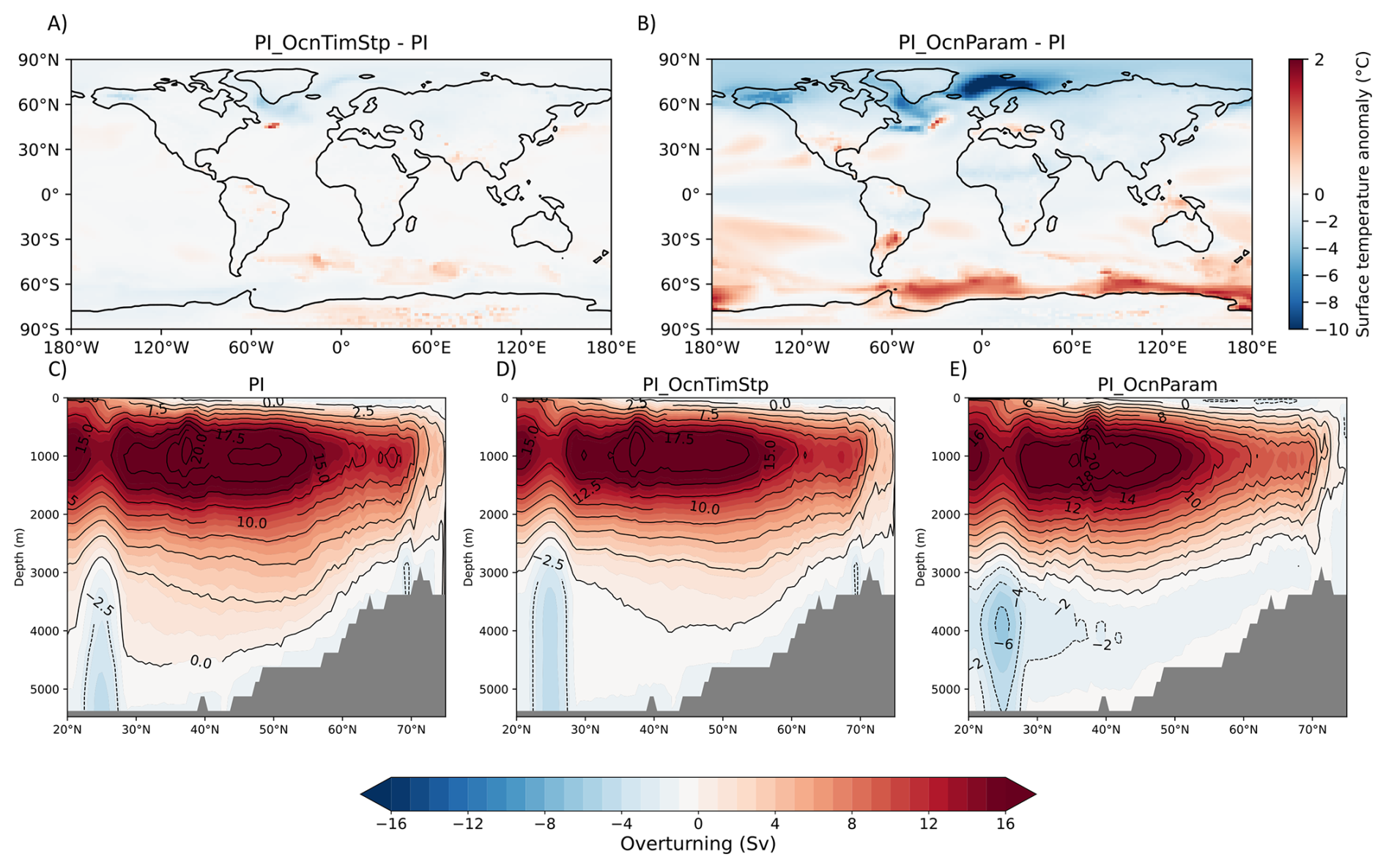
Figure A1 Differences in surface temperatures between PI and (A) PI_OcnTimStp and (B) PI_OcnParam, and AMOC strength at (C) PI, (D) PI_OcnTimStp and (E) PI_OcnParam.

Appendix B: Impact of Antarctic ice sheet on heat transport and radiation

When implementing an Antarctic ice sheet in our mid-Miocene simulations, we observe a global warming and a particularly pronounced warming over the Arctic region. The climate feedbacks coupling the Antarctic ice sheet to Arctic warming is not straightforward, and beyond the scope of our study. However, we would like to highlight here a few elements to motivate future research on the topic.

A first hypothesis was that the ice sheet was somehow causing enhanced heat transport to the Arctic. However, the addition of the ice sheet did not lead to an increase in either oceanic or atmospheric heat transport (Fig. B1). Instead, the difference between atmospheric, oceanic and total heat transport between the simulations is so small, in particular in northern high latitudes, that it suggests local processes are affecting Arctic temperatures.

We compare three processes which are related to climate feedbacks in the Arctic region between the simulations in Fig. B2: effective albedo, ice fraction and longwave cloud forcing. When implementing the Antarctic ice sheet in Mio_Ctrl, we observe an overall reduction of surface effective albedo in the Arctic region (over the ocean and land), a reduction in annual Arctic sea-ice and an increase in longwave cloud forcing. All of these elements would favor a warming of the Arctic region compared to Mio_noIS, by either trapping more heat into the system or decreasing the reflection of shortwaves to space.

From this brief analysis, we are unable to clearly identify the origin of the warming. Climate feedbacks are known to interact with each other, and in particular in the Arctic, there are notable interactions between cloud and sea-ice feedbacks (Kay and Gettelman, 2009), as well as a large role from temperature feedbacks (Pithan and Mauritsen, 2014), with substantial model differences (Block et al., 2020). Therefore, the problem is left open, and could be relevant for questions of polar amplification in warm paleoclimates.

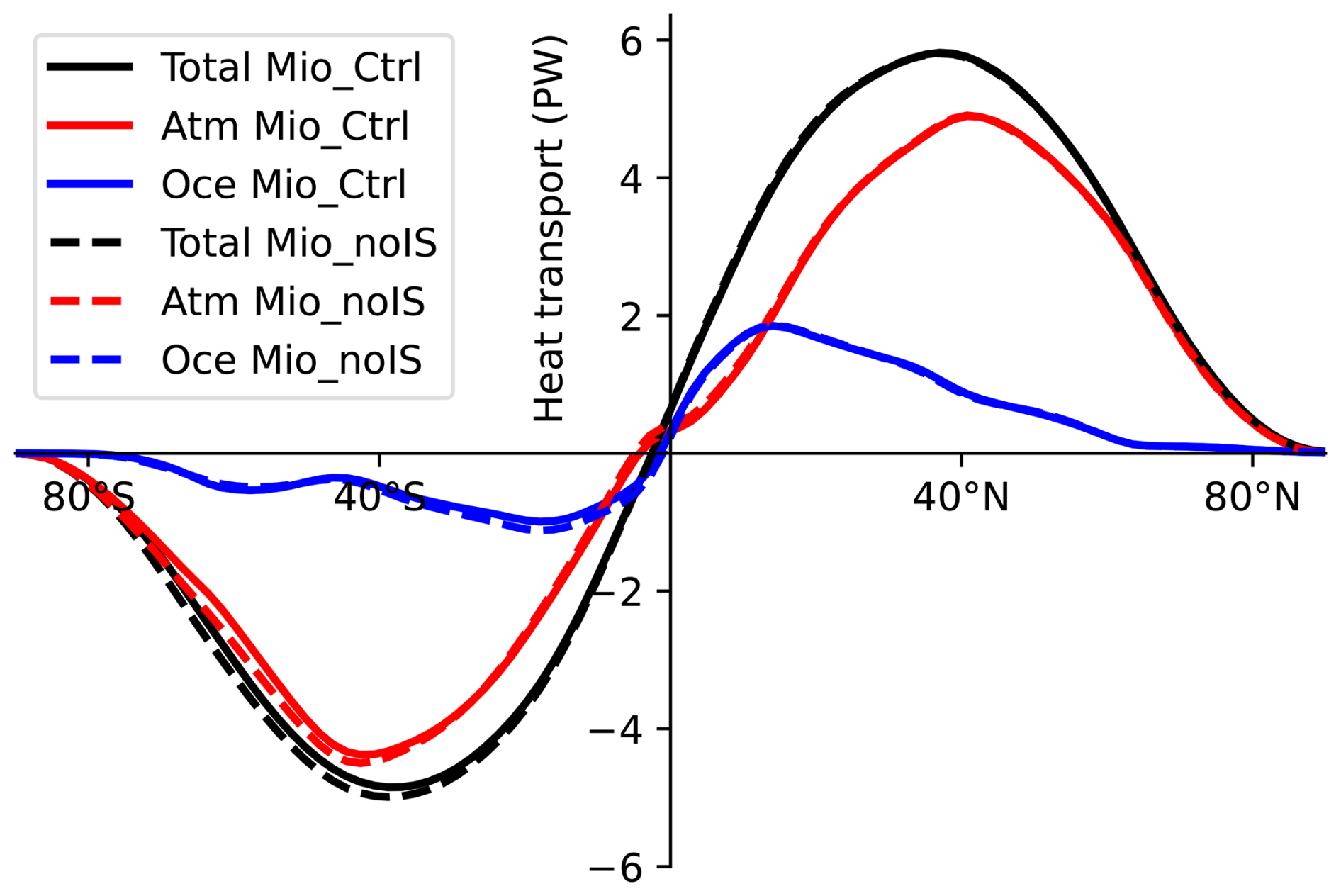
Figure B1 Atmospheric and oceanic heat transports (PW) per latitude between both Mio_Ctrl and Mio_noIS.

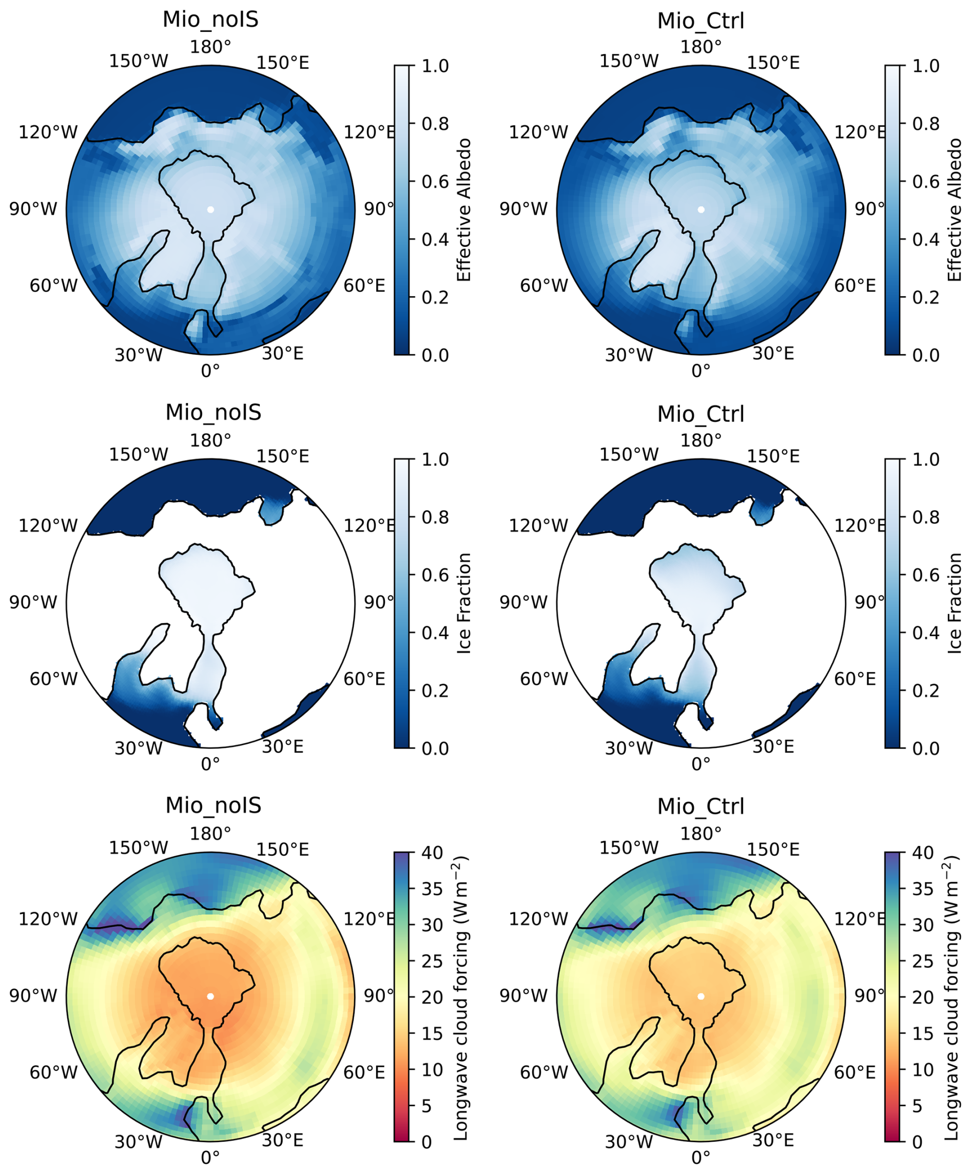
Figure B2 Example of three processes which are tied to climate feedbacks in the Arctic region between Mio_noIS and Mio_Ctrl: effective surface albedo, ice fraction and longwave cloud forcing.