Spatially contrasted response of Devonian anoxia to astronomical forcing

The Devonian period, spanning from 419 to 359 million years ago, was marked by a warmer-than-present climate and recurring ocean anoxic events, with evidence increasingly suggesting a link between these events and astronomical forcing. Here, we explore how astronomical forcing influences ocean oxygenation by modulating the continental weathering flux of phosphate within a Late Devonian climate framework. To investigate this, we performed transient simulations spanning 1.1 Myr, crossing a 2.4 Myr eccentricity node using the cGENIE Earth system model. These simulations were driven by spatially resolved fluxes of reactive phosphorus from continents, computed using the emulator developed by Sablon et al. (2025), trained on GEOCLIM and HadSM3 outputs. Our results provide new evidence supporting eccentricity maxima as a driver of Late Devonian anoxic events. Additionally, global analysis reveals that obliquity variations can leave an imprint on global ocean oxygen levels via their influence on biological productivity, suggesting a potential pathway for obliquity-driven anoxia under greenhouse conditions. Regional analysis revealed pronounced spatial heterogeneity in the biogeochemical response to astronomical forcing. Local ocean circulation emerged as a critical factor in shaping these patterns. The simulations indicate that astronomical forcing can, through its impact on continental weathering fluxes, exert a dominant influence on ocean oxygenation, with regional oxygen concentrations varying by up to 35 % and driving changes in regional anoxic volume of up to 19 %. Finally, these findings help explain why proxy records from different locations may show divergent expressions of astronomical signals, potentially leading to contrasting interpretations of their role in driving ocean anoxia.

1 Introduction

Throughout the Devonian Period, multiple oceanic anoxic events (OAEs) occurred (Becker et al., 2020), with estimated durations ranging from 10⁴ to 10⁶ years (Kabanov et al., 2023). The Late Devonian, approximately 379–360 million years ago (Ma), was particularly marked by pronounced environmental crises and ocean anoxia, such as the well-known Kellwasser and Hangenberg events (Kaiser et al., 2016; Carmichael et al., 2019). There is still no consensus on the mechanisms responsible for the initiation and the duration of these Devonian OAEs (Haddad et al., 2018; Reershemius and Planavsky, 2021; Smart et al., 2023). Existing hypotheses include extensive volcanic activity (Ma et al., 2016; Paschall et al., 2019; Racki, 2020; Kabanov et al., 2023), the proliferation and expansion of terrestrial plants (Algeo and Scheckler, 1998; De Vleeschouwer et al., 2017; Smart et al., 2023), climate cooling (Joachimski and Buggisch, 2002; Song et al., 2017; Huang et al., 2018; Pier et al., 2021), shifts in sea level and oceanic circulation dynamics (Wilde and Berry, 1984; Dopieralska, 2009; Chen et al., 2013), and changes in the position of the continents (Brugger et al., 2019; Gérard et al., 2025). There is also growing evidence that astronomical forcing could modulate at least some of these events, primarily through a “top-down” mechanism (Carmichael et al., 2019) whereby cyclic changes in temperature and precipitation alter continental nutrient fluxes to the ocean (De Vleeschouwer et al., 2014; Martinez and Dera, 2015; De Vleeschouwer et al., 2017; Wichern et al., 2024; Huygh et al., 2025). Specifically, studies conducted in Poland by De Vleeschouwer et al. (2013) identified that the deposition of anoxic black shales associated with the Annulata, Dasberg, and Hangenberg events is separated by approximately 2.4 million years (Myr). This suggests a role of eccentricity in the timing of these events, as the variance spectrum of eccentricity often contains such a cycle (Laskar et al., 2004). However, substantial uncertainties persist regarding the phase relationship of the astronomical forcing to the onset and development of Devonian OAEs. For instance, some cyclostratigraphic interpretations have reported the occurrence of the upper Kellwasser anoxic event, after a 2.4 Myr eccentricity minima (De Vleeschouwer et al., 2017; Da Silva et al., 2020; Wichern et al., 2024), while other studies reported strong obliquity and eccentricity, resulting in marine eutrophication leading to the upper Kellwasser (Ma et al., 2022; Huygh et al., 2025). Hence, these contrasting findings underscore the growing importance of better quantifying the contribution of astronomical forcing to Devonian oceanic oxygen levels and the pathways by which astronomical forcing may have modulated ocean oxygenation at that time.

Our objective is to assess the impact of astronomical forcing on ocean anoxia, specifically through the modulation of continental nutrient fluxes, within a Late Devonian climate context. To this end, we performed transient simulations using the Earth system model of intermediate complexity cGENIE (Ridgwell et al., 2007), coupled offline with a continental weathering flux of nutrients. This flux is computed using an emulator trained on outputs from the general circulation model (GCM) HadSM3 (Valdes et al., 2017) and the geochemical model GEOCLIM (Maffre et al., 2025), as developed in Sablon et al. (2025). By incorporating a GCM, we account for the changes in precipitation and evaporation caused by astronomical forcing more accurately than with the standard version of cGENIE. In addition to improving the representation of hydrological responses, this approach further enhances the simulation of nutrient fluxes to the ocean, limited in the standard cGENIE model version due to its non-dimensional treatment of continental weathering (Colbourn et al., 2013). This modelling framework allows, on the one hand, for a mechanistic assessment of how variations in orbital parameters (namely eccentricity, precession, and obliquity) affect terrestrial weathering rates and nutrient fluxes to the ocean, thereby influencing the development and spatial extent of anoxic conditions. On the other hand, the influence of astronomical forcing on oxygen levels through changes in ocean circulation is captured by cGENIE. A detailed description of the model configuration and experimental design is presented in Sect. 2. In Sect. 3.1, we examine the global characteristics of the transient coupled simulations, followed by a regional analysis in Sect. 3.2.

2 Methods

2.1 Models description

cGENIE is an Earth system model of intermediate complexity (Claussen et al., 2002) designed to simulate long-term interactions between climate, biogeochemical cycles, and ocean–atmosphere processes (Ridgwell et al., 2007). The ocean circulation component (3D) uses a frictional-geostrophic model to simulate the transport of heat, salinity, and biogeochemical tracers through advection, convection, and parametrised mixing. The sea ice module (2D) uses a simplified thermodynamic–dynamic scheme to compute ice thickness and fractional coverage based on thermal balances and surface flux exchanges. The atmospheric module (2D) is an energy–moisture balance layer that transports heat and humidity through advection and diffusion, with precipitation triggered by a humidity threshold. These three components form the C-GOLDSTEIN framework, fully described in Edwards and Marsh (2005) and Marsh et al. (2011). The BIOGEM module simulates ocean biogeochemistry, including nutrient-limited biological productivity and tracer cycling, and handles air–sea gas exchange processes. The ATCHEM module tracks atmospheric chemical species and computes their partial pressures to represent changes in atmospheric composition (Ridgwell et al., 2007). For this study, we used an open-system configuration version of cGENIE with regard to carbon and phosphorus (P), which includes the SEDGEM and ROKGEM modules. SEDGEM provides a representation of sedimentary stratigraphy and the preservation of biogenic carbonates and organic carbon (C_org) deposited on the seafloor (Ridgwell and Hargreaves, 2007; Hülse and Ridgwell, 2025). ROKGEM is a spatially explicit weathering module that simulates temperature- and runoff-dependent weathering rates, allowing dynamic feedbacks between climate, weathering, and the carbon cycle over multimillion-year timescales (Colbourn et al., 2013).

In the standard configuration of cGENIE, continental weathering is simply a function of the global mean continental temperature. This is inadequate to capture the effects of the astronomical forcing, as the latter primarily affects climate through changes in the spatial and seasonal distribution of incoming solar radiation (insolation). To address this, we replaced this simplified scheme with a state-of-the-art continental weathering module, which accounts for the coupled contributions of chemical weathering and erosion. Specifically, we used the framework described in Sablon et al. (2025) to couple cGENIE with a climate–weathering emulator. This emulator computes weathering fluxes under varying boundary conditions (orbital parameters and pCO₂ based on statistical relationships derived from outputs of HadCM3L, HadSM3 (the latter being the slab-ocean version of HadCM3) (Valdes et al., 2017), and GEOCLIM (used with fixed present-day average lithological fractions), explicitly accounting for the coupled contributions of chemical weathering and physical erosion to continental weathering. Both HadCM3L and HadSM3 were used, as the 81 HadSM3 simulations used to train the emulator required heat convergence flux data obtained from HadCM3L. The weathering fluxes are instantaneously routed from continental source cells to the closest ocean coastal grid cell via a nearest-neighbour scheme, which remains suitable given the similar grid layouts, both adapted from Scotese and Wright (2018), and the limited knowledge of the Late Devonian hydrological network. A detailed overview of GEOCLIM’s continental weathering module is presented in Maffre et al. (2025), while a complete description of the emulator’s architecture, training process, and topography is documented in Sablon et al. (2025) and repeated here for clarity (see Fig. 1).

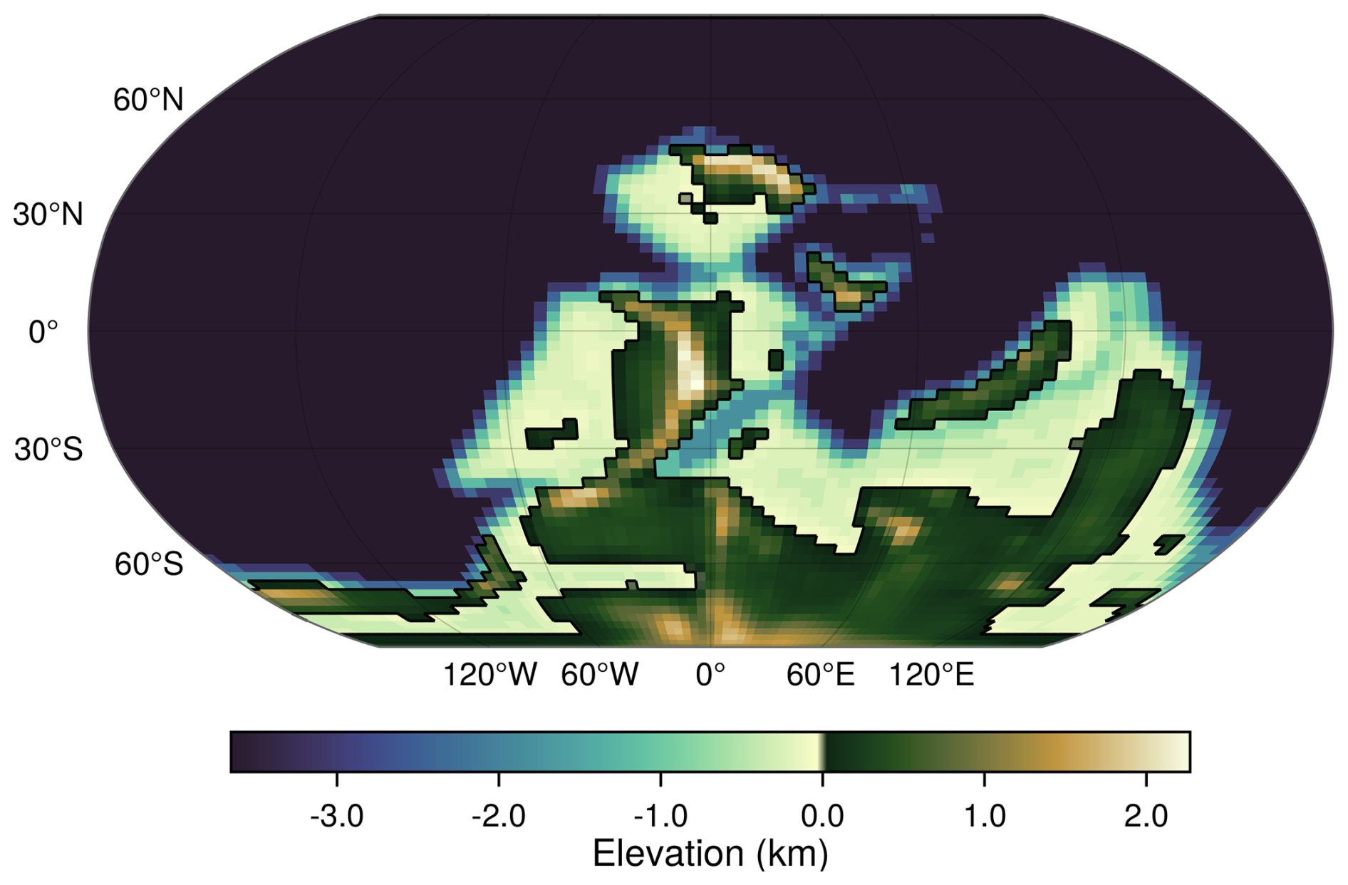
Figure 1 Topography of the Late Devonian (370 Ma). Topography according to Scotese and Wright (2018), reproduced from Sablon et al. (2025). The bathymetry is identical to the one shown in Fig. 2b.

The coupling between the emulator and cGENIE is deliberately minimal and targeted, replacing the continental nutrient flux of dissolved phosphate (PO₄) provided by cGENIE with values computed by the emulator. This replacement is performed offline every 1000 years, a frequency that is appropriate for capturing the long-term variability caused by the astronomical forcing. All other components and processes within the model remain unchanged, as our cGENIE setup uses a simplified, single-nutrient (PO₄) control on biological productivity (Ridgwell et al., 2007). In this configuration, biological productivity is driven by both [PO₄] availability and local insolation. An increase in surface PO₄ availability stimulates biological productivity, thereby enhancing microbial oxygen consumption through remineralization in the water column. Moreover, limiting the coupling to a single flux ensures that other variables computed by ROKGEM remain unaffected, maintaining consistency and simplicity in the overall setup. As a result, cGENIE now responds to spatially-resolved, astronomically-driven variations in continental PO₄ flux, thereby allowing a more robust investigation of the influence of orbital forcing on ocean anoxia.

In our simulations, the ocean is discretised on a 36×36 horizontal equal-area grid with 16 levels along the vertical that are logarithmically spaced (from 60 to 560 m). We use the continental configuration on which the emulator from Sablon et al. (2025) was trained, namely that of Scotese and Wright (2018), which represents the palaeogeography at 370 Ma (see Fig. 2). As this continental reconstruction was also used in Gérard et al. (2025), the large-scale ocean circulation patterns and associated diagnostics described there remain valid here; in particular, the overturning circulation shows only limited sensitivity to temperature changes (see their Fig. 7c). Because the modelled climate system is older than the mid-Mesozoic advent of open-ocean planktic calcifiers (approximately 200 Ma), the representation of calcium carbonate (CaCO₃) production is adapted accordingly (Ridgwell, 2005). Specifically, CaCO₃ production is restricted to shallow-marine carbonate platforms, spatially constrained based on the reconstructions of Kiessling et al. (2003). The surface albedo and zonally averaged wind stress profiles are prescribed from the HadCM3L simulation of Sablon et al. (2025), conducted with the same pCO₂ (926 ppm) as in Valdes et al. (2020) and an orbital configuration characterized by an eccentricity of 0, a longitude of perihelion of 0°, and an obliquity of 23°. These fields are incorporated into cGENIE using the open-source “muffingen” suite v0.9.24 (Ridgwell, 2023), and are held constant throughout the transient simulation. The solar constant is set to 1325 W m⁻² based on Gough (1981), less than today because this younger Sun was also weaker. The atmospheric oxygen concentration is set to 80 % of its present-day value to reflect the lower levels characteristic of the Late Devonian (Krause et al., 2018; Mills et al., 2023). The estimated climate sensitivity of cGENIE is approximately 3 °C per doubling of pCO₂, which is close to the mean value from the Coupled Model Intercomparison Project (CMIP) 5 and slightly lower than that from CMIP6 (Zelinka et al., 2020). Ocean and atmosphere parameter values follow the standard cGENIE setup of Cao et al. (2009) and are identical to those in Pohl et al. (2022) and in Gérard et al. (2025). In our setup, the empirical equation proposed by Dunne et al. (2007) represents C_org burial in marine sediments, while the empirical parameterization of Wallmann (2010) accounts for redox-dependent regeneration of P from sediments. Following Dunne et al. (2007), C_org burial scales with the flux of organic matter reaching the seafloor and is therefore a function of surface ocean productivity. Following Wallmann (2010), a significant portion of P initially bound in organic matter is degraded in surface sediments and released into the ocean as dissolved PO₄. Furthermore, PO₄ release from sediments is enhanced under low-oxygen conditions in line with observations (Ingall and Jahnke, 1994). A detailed description of these schemes and their implementation in cGENIE is provided in Hülse and Ridgwell (2025).

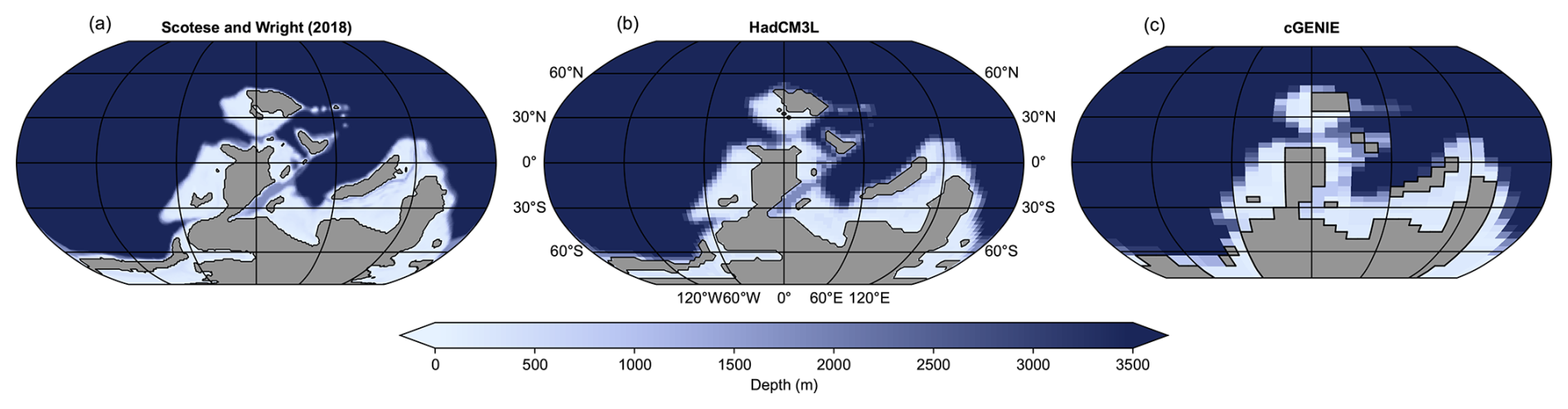
Figure 2 Late Devonian (370 Ma) bathymetry. Comparison between (a) the continental reconstruction from Scotese and Wright (2018), (b) the same reconstruction interpolated onto the HadCM3L model grid used in the emulator, and (c) as per (b) on the cGENIE grid.

2.2 Experimental setup

The astronomical forcing for the Devonian is not known precisely, due to the chaotic nature of the Solar System and the subtle, yet cumulative, effects of tidal dissipation on axial precession (Laskar et al., 2011). A series of plausible solutions is now available (Zeebe and Lantink, 2024), but our experiment design was finalised before that publication appeared. Nevertheless, the astronomical solution employed here shares the same frequency content and amplitude-modulation structure as those found across the Zeebe–Lantink ensemble. We adopted the same hybrid approach as Sablon et al. (2025). It relies, for planetary motion, on the solution by Laskar et al. (2011) (La11a), from which we extracted the interval between 123.3 and 122.2 Ma. This interval features a resonance between the 2.4 Myr eccentricity period (associated with the g4–g3 terms) and the 1.2 Myr obliquity modulation (associated with the s4–s3 terms), as in most of the Cenozoic. This resonance is characterised by an increase in obliquity variance when eccentricity reaches a 2.4 Myr node, at which point its variance is lowest and the 100 000 years (kyr) component of the eccentricity signal disappears. The node occurs approximately midway through the selected interval.

We coupled this solution with the precession model of Sharaf and Boudnikova (1967), following the procedure outlined in Berger and Loutre (1991). This involves first performing a harmonic decomposition of the planetary solution (using R code based on S̆idlichovský and Nesvorný, 1997), and then specifying a reference obliquity and general precession rate. These reference values are given by Farhat et al. (2022) for the period around 370 Ma. With this construction, the solution yields obliquity frequencies of 30.555 and 37.335 years, and climatic precession frequencies of 16.470 and 19.386 years, which are considered plausible for the Late Devonian. The R code used to generate these time series is available in Crucifix (2025). We verified that the time series of obliquity and longitude of perihelion are nearly identical to those obtained by integrating, forward in time, the precession model of Laskar and Robutel (1993) with an appropriate Earth–Moon distance and dynamical ellipticity. The latter approach is admittedly more straightforward, but was not integrated into our workflow at the time the experiment was prepared.

The length and choice of this specific astronomical solution reflect a compromise between representativeness and computational feasibility, given that a 1.1 Myr simulation with cGENIE requires 2 months of continuous computation on our systems. In particular, we cannot know whether the (g4–g3) versus (s4–s3) resonance was active during the Devonian, but previous cyclostratigraphic interpretations assumed a well-expressed 2.4 Myr eccentricity node and pronounced obliquity cycles when crossing the node (De Vleeschouwer et al., 2017). The chosen solution satisfies these assumptions. Moreover, it conveniently includes within a single sequence a transition from well-expressed 100 kyr eccentricity cycles modulated by a 405 kyr cycle, to the 2.4 Myr node (during which the 100 kyr cycles disappear), and then back to well-expressed 100 kyr eccentricity cycles. For reference, we use the heliocentric convention for expressing the longitude of perihelion, which is therefore 0° when perihelion occurs in September (as in Sablon et al., 2025, and Gérard et al., 2025).

cGENIE reached equilibrium through a two-step spin-up process similar to Ridgwell and Hargreaves (2007), Hülse and Ridgwell (2025) and Vervoort et al. (2024). In the initial spin-up phase (SPIN1), ocean dynamics and biogeochemical cycling equilibrate with fixed atmospheric pCO₂ and δ¹³C under a closed system. Burial of CaCO₃, C_org, and P are balanced by global weathering inputs, and the resulting data are used to determine global equilibrium burial rates. The second spin-up phase (SPIN2) uses an open-system setup, with weathering fluxes set to the equilibrium with burial rates from SPIN1 and allowed to respond to temperature. A complete description of this two-step procedure in cGENIE, including C_org and P feedbacks, is detailed in Hülse and Ridgwell (2025). We found that during the SPIN2, the model exhibited significant drift, most notably in pCO₂, with the system requiring up to 500 kyr to reach equilibrium. To address this, we heuristically adjusted the initial pCO₂ concentration in SPIN1 to guide the model toward a geochemically consistent Late Devonian state. Part of this consistency has already been achieved by estimating the initial mean PO₄ concentration based on outputs from GEOCLIM. By the end of SPIN2, the system reached an atmospheric pCO₂ concentration of approximately 550 ppm, consistent with the estimates of Chen et al. (2021) and Dahl et al. (2022), and an average surface PO₄ concentration of 0.47 µmol kg⁻¹, in agreement with Sharoni and Halevy (2023). Furthermore, the system achieved modern-like burial fluxes (similar to Hülse and Ridgwell (2025)), including 0.144 PgC yr⁻¹ of CaCO₃ (reef only) (Frankignoulle and Gattuso, 1993), 0.075 PgC yr⁻¹ of C_org (Dunne et al., 2007; Bradley et al., 2022), and 0.062 Tmol yr⁻¹ of P (Benitez-Nelson, 2000; Ruttenberg, 2003). The cause of this drift remains unclear, but our testing indicates that drift is affected by the continental configuration and model resolution. A full investigation of its origin lies beyond the scope of this study, as it would require substantial computational time, with a 500 kyr simulation requiring roughly 1 month of runtime.

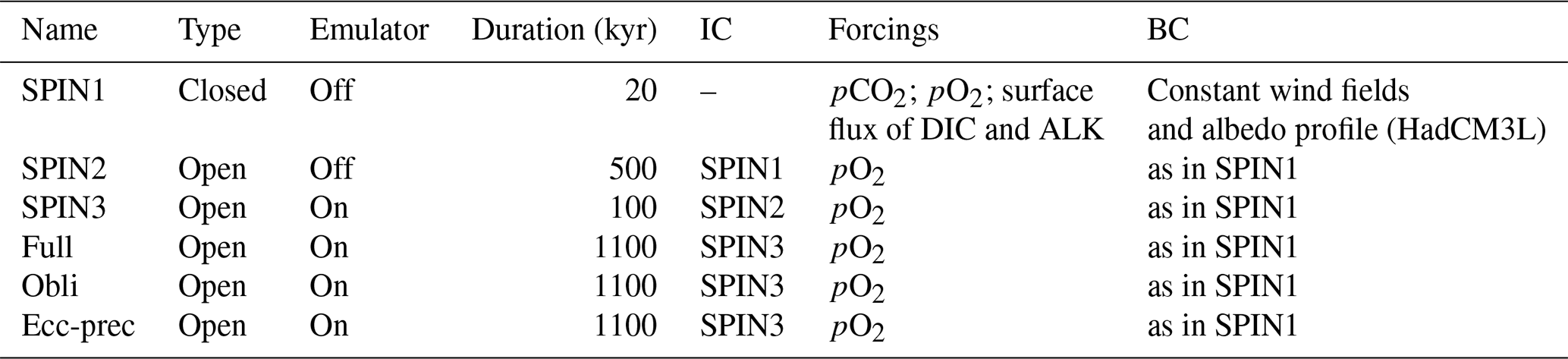
Starting from the equilibrium state (SPIN2), the continental PO₄ nutrient flux provided by cGENIE is replaced with values computed by the emulator. The model is then run for an additional 100 kyr with astronomical parameters fixed at their average value across the adopted astronomical solution, allowing the system to adjust to the new PO₄ flux boundary condition. This average astronomical configuration is characterised by an eccentricity of 0.027, an obliquity of 0.388 rad (22.23°) (Farhat et al., 2022) and longitude of perihelion set to 90° (sin  ϖ=1). To ensure continuity, the global average flux of PO₄ computed by the emulator is rescaled (decreased by approximately 10 %) to perfectly align with the global average flux of PO₄ computed by the built-in weathering module of cGENIE at the end of SPIN2. Following this adaptation period, a series of 3 transient simulations spanning the full 1.1 Myr astronomical solution were conducted. These include: (1) a run with all astronomical parameters evolving (Full); (2) a sensitivity experiment with only obliquity varying while eccentricity and precession were held constant at their average values (Obli); (3) a run in which only eccentricity and precession vary, with obliquity fixed at its average value (Ecc-prec). Simulations description is summarized in Table 1. Additionally, a control simulation was performed in which all astronomical parameters were held constant at their mean values.

Table 1 Experimental design. The type indicates whether the model operates in a closed or open configuration, with the closed setup meaning that every chemical species lost through sedimentation is compensated by an equivalent input from weathering. The emulator is the one from Sablon et al. (2025) that is built on model outputs from HadCM3L, HadSM3, and GEOCLIM. Initial conditions (IC) for SPIN1 are derived from GEOCLIM simulations and include PO₄, alkalinity (ALK), calcium, and sulfate. Forcings correspond to quantities that are explicitly prescribed during the simulations and are the same as in Hülse and Ridgwell (2025). Boundary conditions (BC) are derived from HadCM3L simulations as described in Valdes et al. (2020).

3 Results

3.1 Moderate global astronomical influence

The global time series of atmospheric pCO₂, oceanic PO₄, and dissolved O₂ concentrations ([PO₄] and [O₂] respectively) for each transient simulation conducted across the astronomical solution are shown in Fig. 3. Throughout the reference simulation with all astronomical parameters evolving (black line in Fig. 3), atmospheric pCO₂ fluctuates by up to 40 ppm around a mean value of 555 ppm, driven by interactions within the open carbon cycle (ROKGEM and C_org burial). In the ocean, globally-averaged [PO₄] varies by approximately 0.1 µmol kg⁻¹ around a mean of 2.67 µmol kg⁻¹, while global mean [O₂] remains within a range of 5 µmol kg⁻¹ around an average of 54 µmol kg⁻¹ (see Appendix). The temporal variability of both atmospheric pCO₂ and oceanic [PO₄] is almost exclusively driven by the combined forcings of eccentricity and precession, with obliquity playing a very minor role (see Fig. 3a, b). Overall, variations in global mean concentrations caused by astronomical forcing remain of moderate amplitude. This is consistent with the results of Sablon et al. (2025) and unsurprising considering that global averages can mask spatially heterogeneous responses, including contrasting and potentially compensating regional signals.

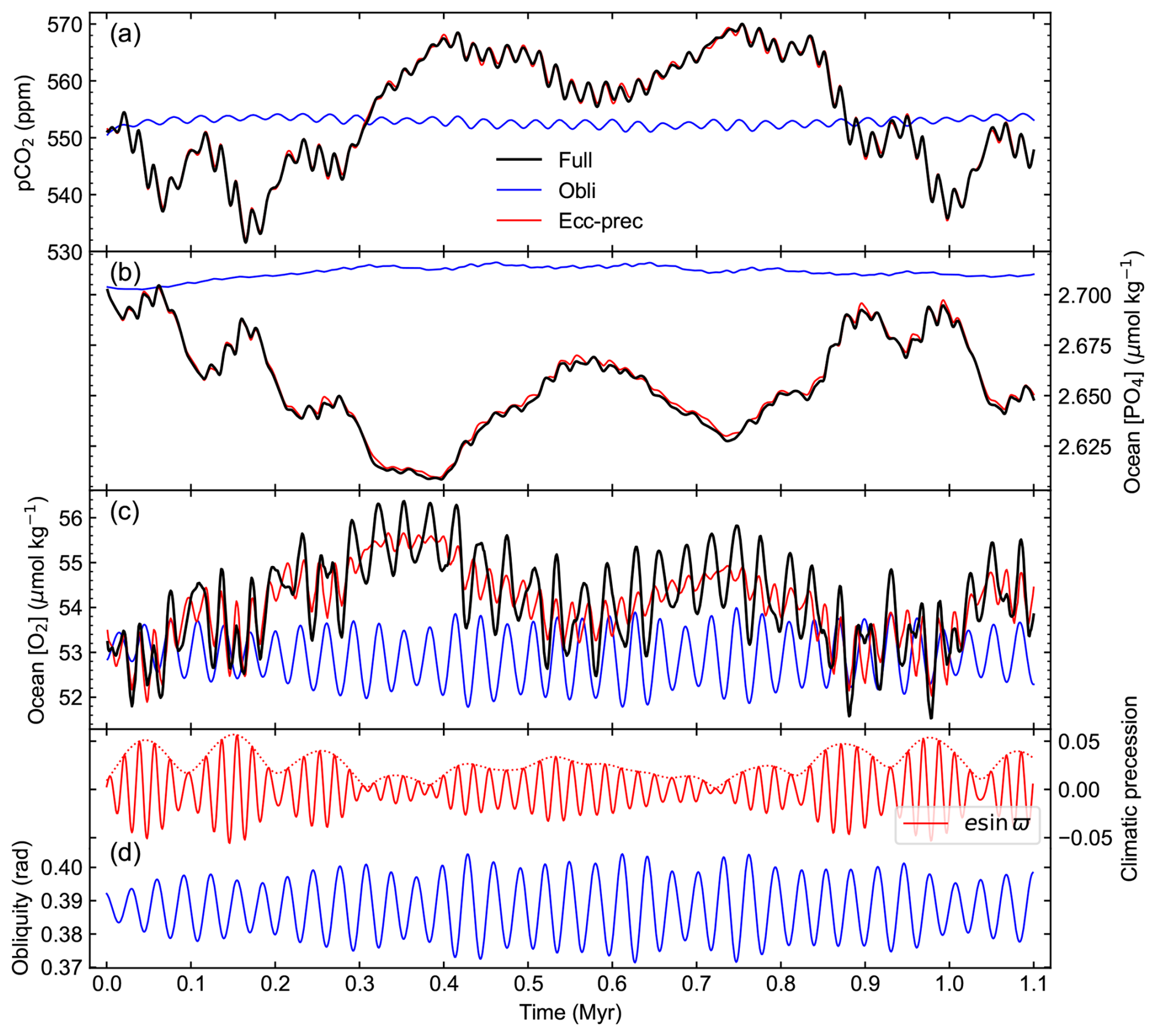
Figure 3 Global response to astronomical forcing. Global time series of (a) pCO₂, ocean (b) [PO₄] and (c) [O₂]. The black curve represents the simulation in which all astronomical parameters evolve. The blue curve represents the simulation with only obliquity varying, while the red curve corresponds to the simulation where only eccentricity and precession evolve. (d) The astronomical solution used in the simulations, with eccentricity in dotted red, climatic precession in red and obliquity in blue. Here, e denotes the eccentricity, and ϖ represents the longitude of perihelion.

Atmospheric pCO₂ and oceanic [PO₄] evolve in anti-phase throughout the simulation (see black and red curves in Fig. 3a, b). This inverse relationship occurs because intensified weathering simultaneously enhances CO₂ consumption and increases the continental flux of PO₄ to the ocean, leading to lower atmospheric pCO₂ and higher oceanic [PO₄]. The dominant control of eccentricity and precession on atmospheric pCO₂ and oceanic [PO₄] arises from their pronounced effect on continental weathering fluxes. Specifically, these two orbital parameters can drive changes in PO₄ delivery to the ocean of up to 9.5 %, compared to only about 1.5 % under obliquity-driven forcing alone. When all three orbital parameters evolve simultaneously, this modulation can reach 10.5 %. In our simulations, the dominant driver is the precession-sensitive monsoon system captured by the emulator: precession alters monsoon intensity and distribution, which directly modulates the spatial pattern of runoff and thus weathering and PO₄ delivery. Beyond this, eccentricity is positively correlated with PO₄ weathering, such that periods of high eccentricity are associated with enhanced oceanic [PO₄], a feature already identified and documented in Sablon et al. (2025).

A global low-oxygen state characterises the ocean in these simulations (see Fig. 3c) compared to the modern climate (Schmidtko et al., 2017; Garcia et al., 2024), consistent with the findings of Gérard et al. (2025) under similar boundary conditions and the estimations made by Tostevin and Mills (2020) based on long-term geochemical proxy data. While all three orbital parameters affect global-mean [O₂], they operate through distinct mechanisms. Eccentricity and precession primarily influence global [O₂] by modulating the oceanic PO₄ inventory. The relationship between globally-averaged [PO₄] and [O₂] is evidenced by a strong correlation (R²= 0.82 and p value = 0.016)¹ between the two red curves in Fig. 3b, c. These [PO₄] variations arise from changes in the continental weathering flux of PO₄, with high eccentricity associated with reduced global [O₂]. In contrast, obliquity exerts only a very weak effect on global [PO₄] that is insufficient to explain the simulated [O₂] variations. This is reflected by the almost absent correlation (R²= 0.06 and p value = 0.467) between the two blue curves in Fig. 3b, c. Instead, obliquity primarily influences global [O₂] through its strong modulation of high-latitude insolation, as also noted by Gérard et al. (2025). Because modelled biological productivity explicitly depends on local insolation (Ridgwell et al., 2007), obliquity substantially alters oxygen consumption in these regions. These variations lead to changes in subsurface (around 60–130 m depth) [O₂] of up to 4 µmol kg⁻¹. As these [O₂] anomalies emerge in deep-water formation zones, they are efficiently distributed throughout the global ocean via large-scale overturning circulation, resulting in consistent oxygen variations of approximately 4 µmol kg⁻¹ across the benthic ocean (not shown). Consequently, times of high obliquity are associated with decreased global [O₂], driven by increased biological productivity in high-latitude regions. There, the productivity anomalies driven by obliquity are more than three times larger than those caused by eccentricity and precession combined. Hence, the combination of high eccentricity and high obliquity results in the most severe depletion of simulated global [O₂] (see Fig. 3c, d).

3.2 High regional variability

To assess regional expressions of [O₂] variability driven by astronomical forcing, we defined distinct regions, as shown together with their associated watersheds in Fig. 4a and b. They are named after their approximate paleogeographic positions: region SA (South America), region WL (western Laurussia), region Si (Siberia), region NP (northern pole), and region LG (Laurussia-Gondwana). These regions were initially constrained by the depth distribution of Devonian anoxia proxy data, which predominantly originates from shallow-marine settings. Because the ocean floor from the Devonian period has been lost to subduction and plate tectonic processes, proxies for deep-water properties are scarce (Granot, 2016; Scotese and Wright, 2018). Consequently, grid cells deeper than 1000 m were excluded, except for those associated with deep-water formation, which occurs in regions SA and NP. Within this depth-limited framework, we further refined the regions by grouping model grid points based on the temporal variance of [PO₄] and [O₂] (see Appendix A), with the final result shown in Fig. 4a. Hence, this approach enables us to assess whether astronomical forcing triggers distinct biogeochemical responses across various regions.

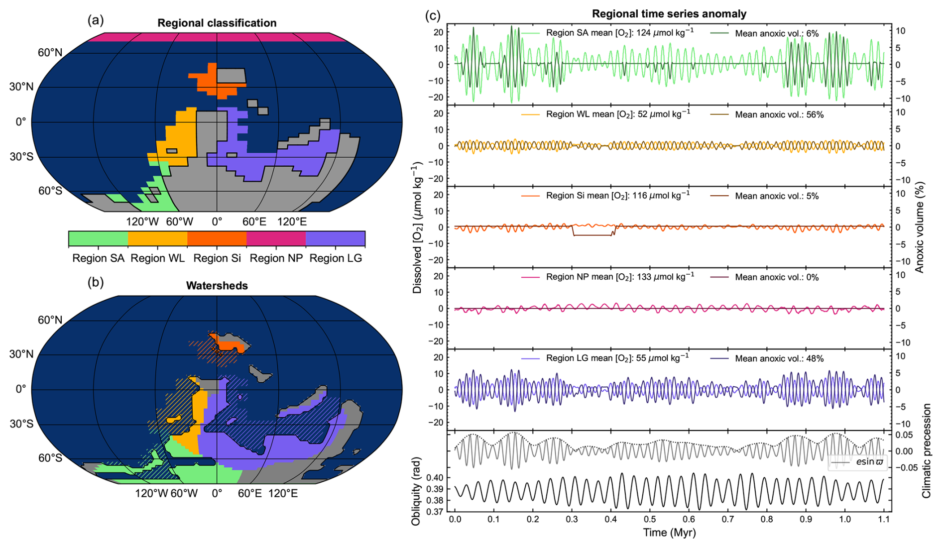
Figure 4 Regional variation of [O₂] and anoxia. (a) Definition of the five regions. (b) Watersheds based on the nearest-neighbour continental runoff routing scheme. The colour of the continental grid cell indicates in which region the weathering flux of PO₄ computed by the emulator of Sablon et al. (2025) is routed. The hashed areas represent the regions as defined in cGENIE and are the same as in panel (a). The discrepancies between the watersheds and the regions arise from the different grid resolution of cGENIE and HadSM3. (c) Time series of average oceanic [O₂] anomalies and anoxic volume anomalies (in %) for each region. These quantities were computed over the full extent of each region, from the second vertical layer down to approximately 1000 m depth, excluding the surface layer as it is in equilibrium with the atmosphere. The anoxic volume is shown in a darker colour, and the anomaly is expressed as a difference of %. The anoxic threshold is set at 6.5 µmol kg⁻¹ after Sarr et al. (2022). For both [O₂] and anoxic volume, the y axis scales are identical across all regional panels to allow direct comparison. As in Fig. 3, the bottom panel displays the astronomical forcing, but shown in black for clarity.

Figure 4c displays the time series of regionally-averaged [O₂] and anoxic volume anomalies, for each region (as defined in Fig. 4a), in the reference simulation with all astronomical parameters evolving concurrently (Full). The results highlight a marked spatial heterogeneity in the biogeochemical response to astronomical forcing. On the one hand, regions SA and LG exhibit strong sensitivity to astronomical variability. In these regions, [O₂] fluctuates by 45 and 19.5 µmol kg⁻¹, respectively, equivalent to a 35 % deviation from their regional means. Simulated [O₂] reach their lowest values during periods of maximum eccentricity. These pronounced oxygen variations translate into substantial changes in anoxic volume, reaching approximately 19 % in region SA and 13.5 % in region LG. On the other hand, region Si is mostly unaffected by astronomical forcing. Temporal variability in both [O₂] and anoxic volume is limited to approximately 5 % and 2.5 %, respectively, with the anoxic volume remaining stable throughout most of the simulation. Although the signal is subtle in magnitude, region Si exhibits an opposite precession phasing compared to regions SA and LG, a feature resulting from their locations in different hemispheres. Region NP exhibits no anoxic conditions over the period, because of its consistently high [O₂] and the limited magnitude of [O₂] variations, which are insufficient for any grid cell in the region to cross the anoxic threshold. These high [O₂] values over region NP are expected given the presence of major deep water formation in this region, whereas the relatively weaker deep water formation in region SA explains why this region can exhibit anoxia (see Figs. A1e and A2).

The relative influence of individual astronomical parameters is clarified by the power spectrum analysis of the [O₂] time series (Fig. 5). Precession emerges as the dominant driver of [O₂] variability in regions SA, WL, Si, and LG, while [O₂] in region NP is primarily shaped by obliquity. Although eccentricity produces no distinct spectral peak, it remains essential through its modulation of precession amplitude (see Fig. 4c). Notably, periods of high eccentricity tend to coincide with decreased oxygen levels across all regions, underscoring its consistent impact.

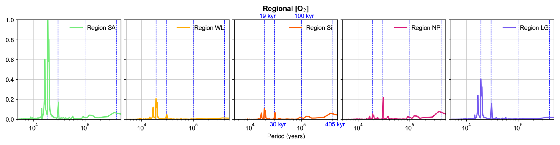
Figure 5 Normalized Fourier power spectrum of the regional [O₂] time series. Vertical dashed lines indicate the characteristic periods of the astronomical parameters: 19 kyr for precession, 30 kyr for obliquity, and 100 and 405 kyr for eccentricity.

By definition, variations in anoxic volume arise from changes in regional [O₂]. Typically, these [O₂] fluctuations are closely tied to changes in biological productivity and subsequent demineralization. In regions SA, WL, and LG, [O₂] variability is almost entirely driven by variations in the [PO₄] component of biological productivity (regional R² ≥ 0.75 and p values $<{\mathrm{10}}^{-\mathrm{3}}$). In region NP, [O₂] variability aligns closely with the insolation component of biological productivity (R² = 0.66 and p value $<{\mathrm{10}}^{-\mathrm{3}}$), whereas the [PO₄] component shows no meaningful relationship (R²=0.01, p value = 0.63). This indicates that insolation-forced biological productivity, rather than [PO₄], controls [O₂] dynamics in this region. Region Si exhibits a distinct behaviour compared with all others. It is the only region where [O₂] variability is not primarily driven by biological productivity (R²=0.22 and p value $<{\mathrm{10}}^{-\mathrm{3}}$), indicating the dominance of another mechanism. The strong correspondence between [O₂] in region Si and the northern hemisphere mean (R²=0.79, p value $<{\mathrm{10}}^{-\mathrm{3}}$) suggests that large-scale physical transport and mixing, consistent with strong currents and circulation in this region (see Fig. 7), drive these regional [O₂] fluctuations. Overall, our results indicate that when regional [O₂] variability is high, it is primarily driven by the [PO₄] component of biological productivity. However, when [PO₄] fluctuations are limited, other processes, such as insolation-forced changes in biological productivity or large-scale advection and mixing, become more critical.

With the link between [PO₄] and [O₂] established, we now turn to the drivers of [PO₄] variability. Figure 6 shows the time series of average [PO₄] and PO₄ weathering, in addition to the linear regression between these two quantities for each region. Region NP has been excluded because there is no direct regional weathering flux of PO₄ coming from the continents. For correlation analysis, the [PO₄] time series for each region (except region Si) was slightly shifted to best align with the weathering time series. This adjustment accounts for the natural time lag between the two quantities, as [PO₄] typically increases when the weathering flux of PO₄ is high. Namely, even as continental weathering begins to decrease, [PO₄] continues to rise as long as the PO₄ input to a given region temporarily exceeds the rate at which it is consumed, producing a lag of several thousand years between the weathering signal and the [PO₄] response (see Fig. 6). To ensure the mechanism remains consistent with an astronomical-forcing interpretation, this lag was chosen to maximize the correlation but was limited to a maximum of 5 kyr (approximately one-fourth of a precession cycle). Because both the magnitude of the PO₄ weathering peak and the rate at which PO₄ is consumed through biological productivity differ across regions, the resulting lag is region-specific. When a negative lag is applied to [PO₄] in regions SA, WL, and LG, it becomes clear that regional weathering accounts for most of the variations in [PO₄]. Hence, in these regions, variations in [O₂] and anoxic extent are predominantly driven by regional [PO₄], hence PO₄ weathering, which in turn is mainly modulated by eccentricity and precession (see Fig. 6).

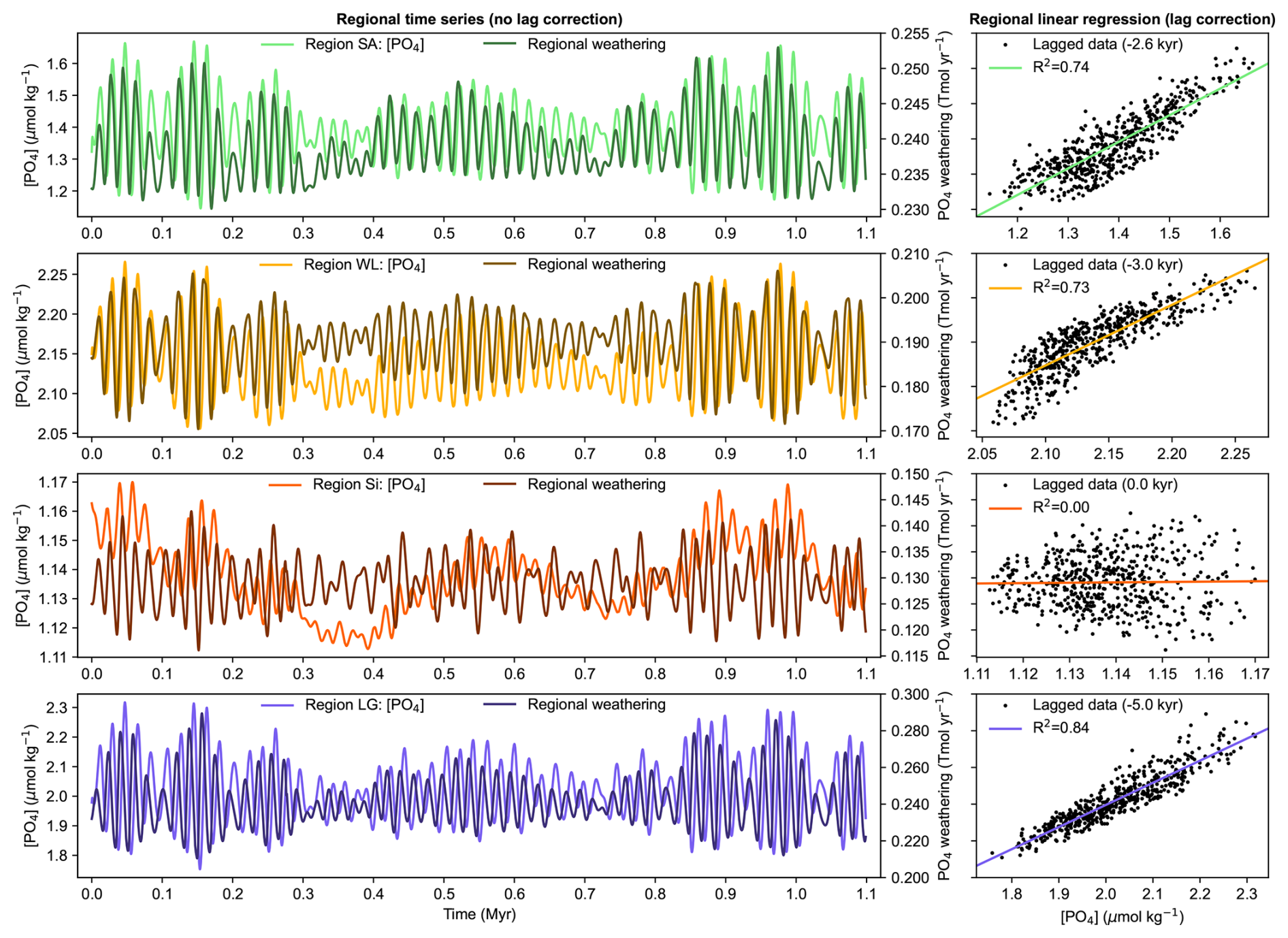
Figure 6 Link between continental PO₄ weathering flux and regional [PO₄]. Displayed are correlations between regional [PO₄] and their corresponding regional weathering fluxes. A negative time lag is applied in the figures on the right, where the regression is computed, and is absent from the figures on the left. Regions SA, WL, and LG have all p values smaller than 10⁻³, while region Si has a p value of 0.35. Region NP is excluded from the analysis due to the absence of direct continental PO₄ weathering.

In region Si, the relationship between [PO₄] and PO₄ weathering differs fundamentally from that of all other regions. Unlike SA, WL, and LG, where regional PO₄ weathering clearly imprints on [PO₄], no meaningful correspondence emerges in region Si. The regional PO₄ weathering flux is comparatively weak (about half that of region LG), and strong currents promote rapid advection and mixing, preventing local accumulation of weathered PO₄ (see Fig. 7). As a result, regional [PO₄] variations do not reflect local weathering input. Instead, [PO₄] in region Si closely follows the broader Northern Hemisphere signal (R²=0.98 and p value $<{\mathrm{10}}^{-\mathrm{3}}$), indicating that large-scale transport governs its temporal evolution. This behaviour is consistent with the mechanism identified earlier: circulation and mixing dominate both [O₂] and [PO₄] variability in region Si.

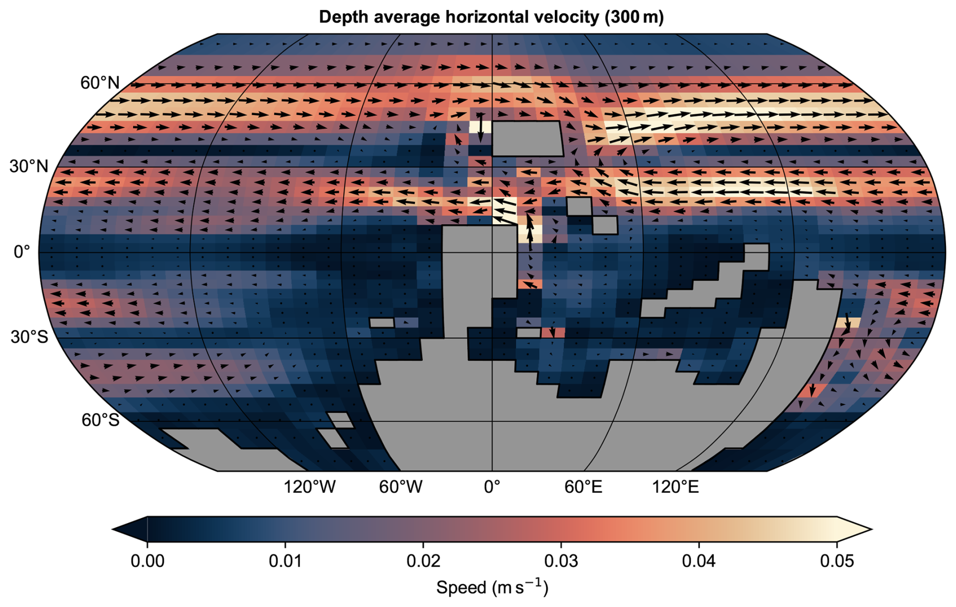
Figure 7 Surface ocean circulation. Mean horizontal ocean velocity (m s⁻¹) averaged over the upper 300 m. Arrow direction indicates flow orientation, while arrow length is proportional to velocity magnitude (also represented with background shading).

4 Discussion

4.1 Implications

We used cGENIE with an upgraded representation of weathering taken from Sablon et al. (2025), to investigate the influence of astronomical forcing on Late Devonian ocean oxygenation. Our simulations show that prescribing plausible atmospheric pO₂ for the Late Devonian (80 % of the modern; Krause et al., 2018, and Mills et al., 2023) leads to an oceanic background state already depleted in [O₂], which likely contributed to the increased frequency of anoxic events observed throughout this period (Becker et al., 2020). We found that astronomical forcing leaves a discernible imprint on the global time series of atmospheric pCO₂, oceanic [PO₄], and dissolved [O₂]. Notably, the evolution of atmospheric pCO₂ under astronomical forcing closely mirrors the results reported by Sablon et al. (2025), exhibiting a similar amplitude of approximately 40 ppm, with higher atmospheric pCO₂ concentrations corresponding to periods of minimum eccentricity. A similar pCO₂ range was also obtained by Vervoort et al. (2024) when running cGENIE with astronomical forcing, using a very different experimental setup featuring an idealized continental configuration and no representation of C_org burial. In our simulations, [O₂] variations primarily occur through the influence of eccentricity and precession on continental weathering fluxes, as well as obliquity on high-latitude biological productivity. Periods of combined high eccentricity and high obliquity produce the most pronounced deoxygenation, although global mean [O₂] variations remain within a modest magnitude range of 5 µmol kg⁻¹ throughout the simulations. Because the ocean exhibits substantial spatial heterogeneity in benthic [O₂], with differences reaching 100 µmol kg⁻¹, it is unlikely for the simulated [O₂] variations to drive global-scale benthic areas below the anoxia threshold. Based on our modelling, it is thus highly implausible that the astronomical forcing alone could induce an anoxic event over the entire global ocean (i.e., including the benthic ocean).

Building on the global-scale analysis, we performed a more localized investigation by defining specific regions to capture potentially distinct biogeochemical dynamics induced by astronomical forcing. The results reveal that eccentricity maxima commonly coincide with the most pronounced anoxic extent, supporting the proposal by Ma et al. (2022) and Huygh et al. (2025) that the Upper Kellwasser coincide with an eccentricity maxima configuration. However, both the magnitude and the dominant astronomical parameter driving this response vary markedly across regions, underscoring the spatial heterogeneity captured in our simulations. While certain regions exhibit strong sensitivity to astronomical forcing, with [O₂] varying by up to 35 % and the anoxic volume by up to 19 %, others remain largely unaffected. Regions near continental margins (i.e., more directly influenced by weathering fluxes) exhibit a strong precessional control, with the largest variations in [O₂] and anoxic volume occurring in these weathering-dominated settings. This influence is not limited to low-latitude areas; for instance, region SA exhibits a notable precession signal despite its relatively high latitude, whereas precession is generally thought to primarily affect low latitudes due to its strong control on precipitation patterns (De Vleeschouwer et al., 2012). In contrast, high-latitude regions far from continental margins (i.e., less directly influenced by weathering fluxes) are more sensitive to obliquity-driven changes, particularly through their influence on the insolation component of biological productivity. These findings underscore the pivotal role of PO₄ weathering and biological productivity in shaping regional biogeochemical responses, aligning with the “top-down” hypothesis proposed in Carmichael et al. (2019). However, physical processes such as ocean circulation and tracer advection can override this control, as exemplified in region Si, where local [O₂] and [PO₄] dynamics are decoupled from regional weathering due to strong transport. Our results further demonstrate how regions SA, WL and LG, characterized by relatively weak surface circulation, provide ideal conditions for astronomically driven weathering variations to leave a substantial imprint on local [O₂].

Altogether, these results demonstrate that astronomical forcing can exert pronounced control on ocean biogeochemistry, with its impact shaped by local physical conditions. Furthermore, the regional analysis of the shallow ocean suggests that an astronomical signal may appear globally distributed across the observational record. However, it also indicates that proxy records from distinct locations may reflect fundamentally different expressions of an astronomical signal, potentially leading to contrasting interpretations of its role in driving ocean anoxia.

Despite the important contribution that astronomical forcing can exert on [O₂], the biogeochemical response of the system remains relatively simple when compared to the forcing. Specifically, the regions often exhibit a quasi-linear response to the forcing, lacking clear signs of long-term memory effects or strong non-linearities. This is particularly surprising given that redox-dependent P regeneration is represented in our model configuration, using the scheme from Wallmann (2010), a feature explicitly proposed in Percival et al. (2020) to explain the sustainability of Late Devonian anoxia based on the investigation of sedimentary concentrations. Hence, the absence of prolonged anoxia in our simulations indicates that the PO₄ variations induced by astronomical forcing may be either too gradual or too limited in amplitude to trigger or maintain an anoxic state over extended timescales in our experimental setup (e.g., 10⁵ years). Our results also suggest that anoxic events could manifest as a series of smaller, short-lived, precession-paced episodes (see Fig. 4c and video in the Supplement) rather than a single, prolonged global event, similar to the scenario proposed by Hedhli et al. (2023). These findings motivate future studies centred on additional processes that may influence the system response, including vegetation–climate interactions driven by orbital forcing and the effects of large, episodic nutrient inputs. In particular, assessing the persistence and biogeochemical consequences of such perturbations could help constrain the conditions under which sustained anoxia might emerge.

4.2 Limitations

Because cGENIE is a relatively simple model, it suffers from well-known intrinsic limitations. Among these are its coarse spatial resolution, resulting in a simplified representation of continental geometry and shallow-water environments, the absence of explicitly resolved atmospheric dynamics, a basic hydrological scheme, and the lack of ice-sheet dynamics. Nevertheless, cGENIE has been widely used in previous studies and has demonstrated its capacity to reproduce large-scale ocean circulation features (Rahmstorf et al., 2005; Lunt et al., 2006; Cao et al., 2009; Marsh et al., 2013; Pohl et al., 2022; Gérard and Crucifix, 2024; Laridon et al., 2025) and to accurately simulate key aspects of ocean biogeochemistry (Ridgwell et al., 2007; Ridgwell and Hargreaves, 2007; Colbourn et al., 2013; Ward et al., 2018; Adloff et al., 2020; Reinhard et al., 2020; Crichton et al., 2021; van De Velde et al., 2021; Naidoo-Bagwell et al., 2024; Stappard et al., 2025). These studies collectively demonstrate the model’s reliability in simulating paleoclimate conditions and associated biogeochemical responses. Furthermore, some of these limitations are addressed by our specific experimental design. The prescribed wind stress field, although not responsive to climate variability, was derived from HadCM3L simulations conducted by Sablon et al. (2025). Hence, further assessments of the impact of dynamically evolving wind stress and albedo fields under astronomical forcing, through dedicated experiments specifically designed to isolate and quantify these effects, would be valuable, particularly using higher-complexity models (e.g., IPSL). This is further encouraged by the results of Sarr et al. (2022), who showed that astronomically driven changes in ocean circulation and ventilation can exert a strong control on oxygenation, with regional variations reaching up to 40 µmol kg⁻¹ in a Late Cretaceous context. More generally, the emulator accounts for changes in precipitation associated with variations in astronomical configuration and atmospheric pCO₂, thereby improving the representation of hydrological controls on PO₄ weathering. Together, these features enable a more realistic representation of two central climate components in our study: PO₄ weathering and ocean circulation.

Still, several important limitations of our approach carry implications for interpreting the results. Our results could depend on the selected paleogeographic reconstruction, given the substantial uncertainties that persist in deep-time topography and, by extension, in slope, erosion, and weathering patterns. It would therefore be valuable for future studies to assess how alternative reconstructions, such as those from Vérard (2019) or Cermeño et al. (2022), might influence these processes and the resulting oceanic response. Moreover, a simple nearest-neighbour scheme was used to route continental weathering products into the ocean; alternative watershed configurations could yield significantly different regional responses to astronomical forcing. Similarly, the use of HadCM3L, HadSM3, and GEOCLIM necessarily reflects one possible representation of climate and weathering dynamics; alternative emulator models or hydrological schemes could yield quantitatively different outcomes, although assessing the magnitude of such differences would require dedicated sensitivity experiments. The current setup also does not capture extreme events that may substantially influence sedimentary fluxes, and relies on a simplified organic matter sedimentation scheme that lacks oxygen dependence, highlighting the potential benefit of integrating more advanced models of organic matter diagenesis like OMEN-SED (Hülse et al., 2018) in future work. Additionally, the surface wind stress field is held constant throughout the simulations, preventing realistic changes in circulation patterns in response to evolving astronomical configurations. The exclusion of ice sheets and sea-level variations removes critical mechanisms through which obliquity can strongly impact [O₂], although the accurate representation of sea-level changes would remain challenging at the cGENIE grid resolution. Several studies have suggested that these processes may have contributed to, or exacerbated, Late Devonian anoxic events (Bond and Wignall, 2008; Chen et al., 2013; Huygh et al., 2025). As a result, the influence of obliquity identified in this study may be underestimated, though it still leaves a discernible imprint on the global ocean. For all these reasons, we emphasize the importance of further modelling efforts to better connect orbital forcing with ocean anoxia. For instance, subsequent work would benefit from incorporating dynamic albedo and wind-stress profiles when exploring the full range of climate–circulation–biogeochemistry interactions. They could also explicitly test the robustness of the Late Devonian background state and its sensitivity to evolving external forcing across multiple models. In this context, Earth System Models of Intermediate Complexity (EMICs) offer a promising path forward, as they allow for long-timescale simulations while explicitly resolving many key physical and biogeochemical processes.

5 Conclusions

We have explored the role of astronomical forcing in driving ocean anoxia under a Late Devonian climate configuration. Our experimental setup relies on an offline coupling between cGENIE and a fast climate-weathering emulator, based on a GCM, developed by Sablon et al. (2025). It allowed us to capture the influence of astronomical forcing on oceanic [O₂] via its modulation of continental PO₄ weathering fluxes. At the global scale, astronomical forcing exerts a moderate impact on ocean [O₂], with the most pronounced deoxygenation occurring during intervals of combined high eccentricity and high obliquity. While eccentricity and precession primarily affect [O₂] through their control on PO₄ weathering fluxes, obliquity exerts its influence by modulating the insolation component of biological productivity at high latitudes, highlighting that even in a greenhouse world, obliquity can leave an imprint on ocean biogeochemistry, hence possibly sedimentary records. At the regional scale, eccentricity maxima also correspond to the most extensive anoxic conditions, providing new evidence supporting a strong impact of eccentricity maxima on the development of Late Devonian anoxic events. However, the biogeochemical response remains highly variable across regions. Our results show that astronomical forcing can act as a dominant control on ocean [O₂], driving regional changes in anoxic volume of up to 19 %. An unanticipated result is that local ocean circulation can represent a central driver of the spatial heterogeneity in [O₂] responses to astronomical forcing. As a result, sedimentary records from different locations may reflect contrasting imprints of the same astronomical signal, potentially leading to contrasting interpretations of its role in pacing Late Devonian anoxia. Finally, while this study provides insights into how astronomical forcing affects Late Devonian ocean [O₂], it also stresses the difficulty of explaining the duration of Devonian anoxic events and the uncertainties in their spatial extent, underscoring that much modelling and data integration work remains to fully understand the drivers and dynamics of Late Devonian anoxia.

Appendix A: Background state and ocean circulation

Figure A1a, b, and d show a strong hemispheric asymmetry in oxygenation, with a substantially more oxygenated Northern Hemisphere compared to the Southern Hemisphere. This pattern primarily reflects large-scale ocean circulation (Fig. A1e), which allows well-oxygenated surface waters to ventilate the deep ocean in the Northern Hemisphere. In contrast, a pronounced oxygen minimum zone (OMZ) develops across much of the Southern Hemisphere (Fig. A1d), where meridional overturning circulation is nearly absent. The OMZ is shallower towards low latitudes, where primary productivity is high, consistent with enhanced biological oxygen demand (Fig. A1c). Primary productivity is also relatively elevated at high latitudes, while minimum values occur at mid latitudes, where downwelling associated with subtropical gyres prevents primary productivity. The seafloor [O₂] map further indicates that most anoxic conditions at the seafloor are restricted to shallow ocean regions, as confirmed by comparison with the model bathymetry (Fig. 2c). These shallow regions therefore correspond to areas where sedimentary P regeneration feedbacks are expected to be strongest.

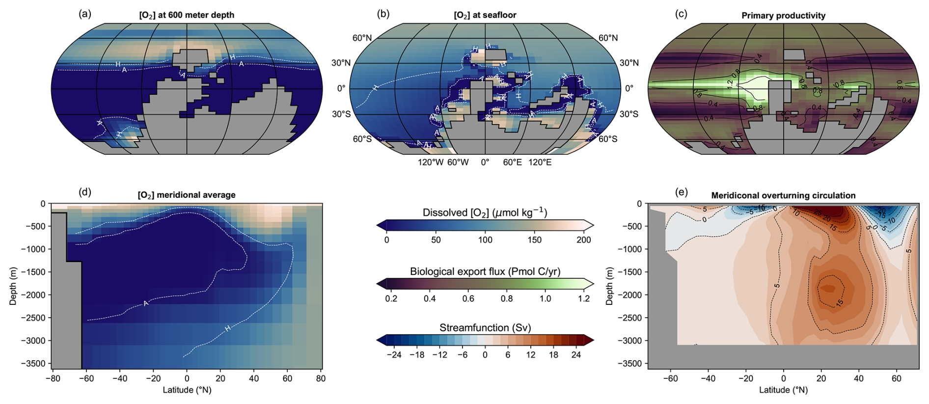
Figure A1 Background state at the end of SPIN3. [O₂] at a depth of 600 m (a) and at the seafloor (b). (c) Primary productivity (Pmol C yr⁻¹). (d) Meridional average of [O₂]. (e) Meridional overturning streamfunction (1 Sv ≡ 10⁶ m³ s⁻¹). The white dashed lines in (a), (b), and (d) indicate the boundaries for the anoxic (A) and hypoxic (H) regions, with threshold values taken after Sarr et al. (2022).

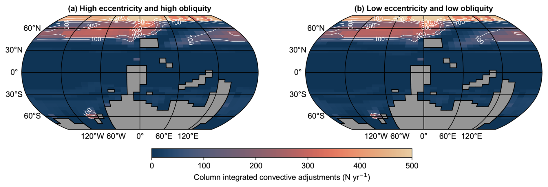
Figure A2 Deep water formation. Convective adjustments (expressed as the number of convective adjustments integrated across the water column per year) for (a) high eccentricity-high obliquity and (b) low eccentricity-low obliquity astronomical configurations.

Changes in ocean circulation associated with astronomical forcing are small in our simulations, with a maximum variation in overturning strength of 0.7 Sv (Sverdrup) when all orbital parameters vary together (0.56 Sv for eccentricity-precession forcing and 0.32 Sv for obliquity alone). Figure A2 further indicates that the main regions of deep-water formation remain largely unchanged between extreme orbital configurations (extracted from the 1.1 Myr transient simulation). This small variability likely reflects the absence of dynamical changes in ocean circulation associated with orbital variations across the simulations. It may also indicate that the large-scale ocean circulation in cGENIE is not sufficiently sensitive to variations in surface albedo and wind stress forcing. Overall, the spatial distribution of deep-water formation explains the global overturning circulation pattern shown in Fig. A1e.

Appendix B: Defining regions

This section clarifies how we refined the definition of the different regions based on the temporal variance of [O₂] and [PO₄]. Figure B1 shows the normalized temporal variance of these two tracers, averaged over the upper 1000 m, consistent with the depth range applied in our regional analysis (see Sect. 3.2). First, a clear distinction between regions SA and WL emerges from both [O₂] and [PO₄] variance fields, particularly around 30° S and 60° W, providing strong justification for separating them. Second, region LG was initially split into two sub-regions based on the spatial structure of the variance fields. However, the temporal evolution and variability of [O₂], anoxic volume, and [PO₄] were found to be highly consistent across these sub-regions. Consequently, we merged them into a single, unified region, which we now refer to as region LG. These refinements provide a clear and consistent basis for the regional definitions presented in Fig. 4a. Although regional boundaries are somewhat arbitrary, they follow coherent patterns of variability and are broad enough to avoid overinterpreting hyper-localised phenomena (at the single grid cell level). The resulting regions are not intended as universal classifications, but rather as a practical framework for exploring the spatial heterogeneity of climate–biogeochemical interactions.

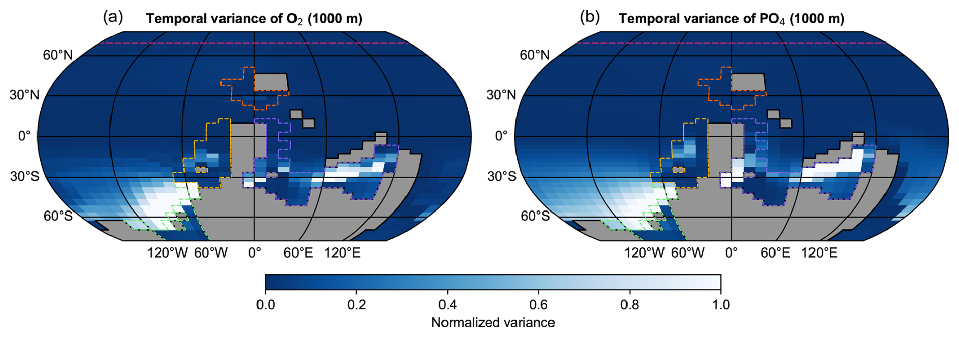
Figure B1 Temporal variance. Normalized temporal variance of (a) [O₂] and (b) [PO₄] averaged over the upper 1000 m. Dashed coloured lines indicate regional boundaries, as defined in Fig. 4.