Patterns of changing surface climate variability from the Last Glacial Maximum to present in transient model simulations

As of 2023, global mean temperature has risen by about 1.45±0.12 °C with respect to the 1850–1900 pre-industrial (PI) baseline according to the World Meteorological Organization. This rise constitutes the first period of substantial global warming since the Last Deglaciation, when global temperatures rose over several millennia by about 4.0–7.0 °C according to proxy reconstructions. Similar levels of warming could be reached in the coming centuries considering current and possible future emissions. Such warming causes widespread changes in the climate system, of which the mean state provides only an incomplete picture. Instead, fluctuations around the mean and in higher-order statistics need to be considered. Indeed, climate's variability and the distributions of climate variables change with warming, impacting, for example, ecosystems and the frequency and intensity of extremes. However, previous investigations of climate variability focus mostly on measures such as variance, or standard deviation, and on quasi-equilibrium states such as the Holocene or Last Glacial Maximum (LGM). Changes in the tails of distributions of climate variables and transition periods such as the Last Deglaciation remain largely unexplored.

Therefore, we investigate changes of climate variability on annual to millennial timescales in 15 transient climate model simulations of the Last Deglaciation. This ensemble consists of models of varying complexity, from an energy balance model to Earth system models (ESMs), and includes sensitivity experiments, which differ only in terms of their underlying ice sheet reconstruction, meltwater protocol, or consideration of volcanic forcing. The ensemble simulates an increase in global mean temperature of 3.0–6.6 °C between the LGM and Holocene. Against this backdrop, we examine whether common patterns of variability emerge in the ensemble. To this end, we compare the variability in surface climate during the LGM, Deglaciation, and Holocene by estimating and analyzing the distributions and power spectra of surface temperature and precipitation. For analyzing the distribution shapes, we turn to the higher-order moments of variance, skewness, and kurtosis. These show that the distributions cannot be assumed to be normal, a precondition for commonly used statistical methods. During the LGM and Holocene, they further reveal significant differences, as most simulations feature larger temperature variance during the LGM than the Holocene, in line with results from reconstructions.

As a transition period, the Deglaciation stands out as a time of high variance in surface temperature and precipitation, especially on decadal and longer timescales. In general, this dependency on the mean state increases with model complexity, although there is a large spread between models of similar complexity. Some of that spread can be explained by differences in ice sheet, meltwater, and volcanic forcings, revealing the impact of simulation protocols on simulated variability. The forcings affect variability not only on their characteristic timescales. Rather, we find that they impact variability on all timescales from annual to millennial. The different forcing protocols further have a stronger imprint on the distributions of temperature than precipitation. A reanalysis of the LGM exhibits similar global mean variability to most of the ensemble, but spatial patterns vary. However, paleoclimate data assimilation combines model and proxy data information using a Kalman-filter-based algorithm. More research is needed to disentangle their relative impact on reconstructed levels of variability. As such, uncertainty around the models' abilities to capture climate variability likewise remains, affecting simulations of all time periods: past, present, and future. Decreasing this uncertainty warrants a systematic model–data comparison of simulated variability during periods of warming.

1 Introduction

Understanding the response of the climate system during extended periods of global warming is of vital importance given current and projected anthropogenic warming. However, the observational record provides an insufficient data basis due to its short length of only about 150 years and its sparse spatial coverage during the earlier years (e.g., Morice et al., 2012). To extend the record further back in time requires the use of natural climate archives and proxy-based reconstructions. Such reconstructions have many associated uncertainties and limited resolution in time and space. Combining proxy records from different locations into a global field reconstruction introduces additional uncertainties, such as different interpolation and calibration procedures, age models, and proxy biases (Christiansen and Ljungqvist, 2017; Tingley et al., 2012). Climate models, on the other hand, simulate three-dimensional fields of a wide variety of variables that describe the climate. As such, they provide continuous estimates of climate that are limited by model physics and parametrizations but allow detailed investigations of the climate system and its changes on long timescales. Since their simulation length and resolution depend mostly on computational resources, simulation protocols up until the Paleoclimate Modeling Intercomparison Project phase 3 (PMIP3) encompassed mostly equilibrium simulations of past climate states in the form of time slices. Experiments with time-dependent (transient) forcings were limited to short periods like the past millennium or done with accelerated boundary conditions. The latest iteration, PMIP4, added more and longer experiments with transient boundary conditions. This allows more in-depth explorations of past transitions in the climate's mean state, such as the Last Deglaciation, which we examine here using an ensemble of transient simulations.

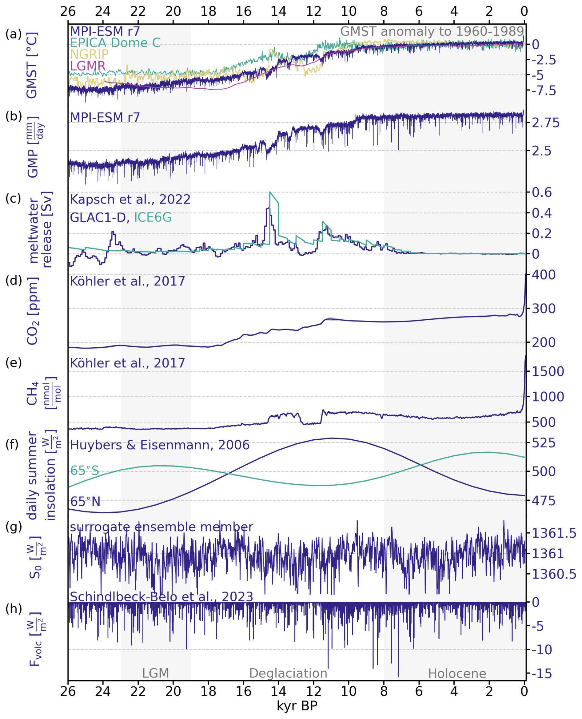
Figure 1 Climate responses and external forcing during the past 26 kyr: (a) global mean temperature anomaly (with regard to 1960–1989) as simulated by MPI-ESM, captured in ice cores from Antarctica (EPICA Dome C; Jouzel et al., 2007) and Greenland (NGRIP; Andersen et al., 2004) and reconstructed in the LGM reanalysis (Osman et al., 2021). The proxy records for local temperature derived from EPICA and NGRIP are scaled to GMST using GMST$=\mathrm{0.5}\times {\mathrm{T}}_{\mathrm{local}}$. (b) Global mean precipitation as simulated by the Earth system model MPI-ESM, (c) meltwater release for ice sheet reconstructions GLAC1-D and ICE6G as used in MPI-ESM r1–r7 (Kapsch et al., 2022), (d) atmospheric CO₂ (Köhler et al., 2017) and (e) CH₄ levels (Köhler et al., 2017), (f) daily insolation at 65^∘N and 65^∘S at the summer solstice (Huybers and Eisenman, 2006), (g) solar constant from one ensemble member generated as surrogate data based on Steinhilber et al. (2009) following Ellerhoff and Rehfeld (2021) (comparison with Steinhilber et al., 2009 in Fig. S2 in the Supplement), and (h) volcanic forcing TephraSynthIce (Schindlbeck-Belo et al., 2024; Sigl et al., 2022).

As the transition from the Last Glacial Maximum (LGM; 23–19 kyr before present¹) to the current warm period of the Holocene (10.65 kyr BP–present day), the Last Deglaciation was a period of substantial global climate change. Global mean surface temperature (GMST) increased by about 4–7 °C according to proxy-based reconstructions and climate model simulations (Fig. 1a; Gulev et al., 2021; Osman et al., 2021; Annan et al., 2022; Tierney et al., 2020; Shakun and Carlson, 2010). The spread among recent estimates is similar, with some leaning towards the higher end with a warming of 7.0 ± 1.0 °C suggested by Osman et al. (2021) and 6.1 °C (5.7, 6.5) by Tierney et al. (2020) and others towards the lower end such as the estimate of 4.5 ±0.9 °C by Annan et al. (2022). In simulations, a rise in global mean precipitation (GMP) accompanies this warming (Fig. 1b). During the same period, global mean sea level rose by approximately 120 m as the ice sheets in both hemispheres, but especially the Fennoscandian and Laurentide ice sheets, shrunk (Fig. 1c, Lambeck et al., 2014; Grant et al., 2012). However, there are significant uncertainties associated with ice sheet reconstructions, especially with respect to ice sheet extent and elevation (Stokes et al., 2015; Abe-Ouchi et al., 2015; Ivanovic et al., 2016). In turn, the timing and magnitude of meltwater events, which crucially impact the deglacial climate evolution (Snoll et al., 2024), remain uncertain.

Increasing levels of atmospheric carbon dioxide (CO₂) contributed to and drove this change (Shakun et al., 2012) as they rose from about 193.2 ppm at the onset of the Last Deglaciation to approximately 271.2 ppm at its end (Gulev et al., 2021). During the Holocene, CO₂ levels roughly stabilized until the Industrial Revolution (Fig. 1d). Similarly, atmospheric methane almost doubled from the LGM to the Holocene (Köhler et al., 2017, Fig. 1e). Changes in latitudinal and seasonal insolation distribution favored this rise in atmospheric greenhouse gases (GHGs) and warming (Fig. 1f).

However, considering only the described mean changes is insufficient to capture the full breadth of climate change then and now. Instead, it is necessary to study the climate's variability, too, as reflected in the fluctuations around the mean² and in higher-order statistics in space and time (Katz and Brown, 1992). These fluctuations determine the actual climate conditions at any point in time and space and are the focus of our study. They affect the various modes of variability (Rehfeld et al., 2020) and the occurrence and frequency of extremes (Simolo and Corti, 2022; Ionita et al., 2021; Schär et al., 2004; Loikith et al., 2018; Ruff and Neelin, 2012; Laepple et al., 2023). Climate variability further acts across timescales, from intra-annual (i.e., heat waves) and interannual (multi-year droughts, the El Niño–Southern Oscillation (ENSO)) to millennial scales (D–O events) and beyond and across different spatial scales (Franzke et al., 2020; Laepple et al., 2023).

Proxy-based reconstructions suggest that global mean temperature variance was about 4 times higher during the LGM than the Holocene, possibly due to changes in the Equator-to-pole temperature gradient (Rehfeld et al., 2018). This implies a dependence of variability on mean climate. The extent of this state dependency varies regionally; e.g., Rehfeld et al. (2018) find that it is generally larger in the Northern Hemisphere mid- and high latitudes than in the Southern Hemisphere. Models are only partially able to match this LGM-to-Holocene change in temperature variability. Rehfeld et al. (2018) found that interannual to decadal variability is about 30 % higher during the LGM than during the pre-industrial (PI) in PMIP3 and Coupled Model Intercomparison Project (CMIP) phase 5 simulations. Shi et al. (2022) confirmed this for PMIP3/4 LGM simulations, which have about 20 % larger interannual variability than PI simulations. Models do agree with reconstructions on decreasing global temperature variability (Rehfeld et al., 2020) and mean local variability (Ellerhoff et al., 2022) with warming, especially towards higher latitudes (Ellerhoff et al., 2022), but with some exceptions in the tropics (Rehfeld et al., 2020). Few studies quantitatively considered variability changes over the Last Deglaciation. One, Weitzel et al. (2024), compared millennial and orbital variability in many of the transient simulations considered here with proxy reconstructions. Differences varied in time and space, and no single simulation was identified to best match reconstructions.

Globally, there is mostly agreement between the variance at interannual to centennial timescales in models and reconstructions both during the Holocene (Laepple et al., 2023) and further back in time, including during the Deglaciation (Zhu et al., 2019). On regional and local scales, however, models simulate less variability than reconstructions, especially on multi-decadal timescales and longer (Laepple et al., 2023; Ellerhoff et al., 2022; Rehfeld et al., 2018). Including natural forcing (that is, forcing from solar and volcanic activity) in simulations reduces this difference but cannot close it (Ellerhoff et al., 2022). Opposite to temperature, precipitation variability increases with warming, with some regional exceptions (Rehfeld et al., 2020). This precipitation variability can be linked to mean precipitation changes, as dry regions generally have lower variability and wet regions generally have higher variability (Rehfeld et al., 2020).

The influence of natural forcing demonstrates that significant variability arises in response to external forcings and boundary conditions. Volcanism, in particular, has been identified as a prominent driver of changes in temperature, precipitation, and modes of atmospheric dynamics (Timmreck, 2012; Iles and Hegerl, 2015; Liu et al., 2016; Zanchettin et al., 2015). Its strongest effects manifest on annual timescales (Lovejoy and Varotsos, 2016), as has been found for the past millennium and Common Era (Schurer et al., 2014; Lovejoy and Varotsos, 2016). It further contributed substantially to subdecadal (Le et al., 2016), decadal (Hegerl et al., 2003), and multi-decadal (Schurer et al., 2013) variance. During glacials, strong volcanic eruptions are even suggested as a driver of millennial variability (Baldini et al., 2015). There is conflicting evidence with respect to the dependence of the impacts of volcanic forcing on the background state: in equilibrium simulations of the LGM and the PI period, Ellerhoff et al. (2022) found no state dependency on the global scale for surface temperature variability and only slight differences for precipitation. Bethke et al. (2017), on the other hand, found enhanced variability in future projections on annual to decadal timescales.

Throughout glacial cycles, the cryosphere plays a crucial role for the climate and its variability. This includes sea ice dynamics and changes in ice sheets and associated meltwater releases. Ice sheets and meltwater releases are still commonly simulated as external forcings (Ivanovic et al., 2016). However, reconstructions of ice sheet extent and elevation and associated meltwater pulses entail significant uncertainties (Stokes et al., 2015; Abe-Ouchi et al., 2015; Ivanovic et al., 2016; Izumi et al., 2023). For both the LGM and the Last Deglaciation, simulated climate has been shown to be very sensitive to ice sheet reconstructions (Izumi et al., 2023; Kapsch et al., 2022; Bakker et al., 2020; Ullman et al., 2014). Furthermore, meltwater release as a consequence of melting ice sheets affects ocean circulation and thus deglacial climate as a whole (Kapsch et al., 2022). Consequently, the uncertainties in meltwater scenarios and models' varying sensitivities to freshwater crucially affect the simulation of deglacial climate (Snoll et al., 2024).

For sea ice, a decreasing extent has been shown to reduce the seasonal to interannual standard deviation of temperature, likely due to polar amplification and the sea ice–albedo feedback (Screen, 2014; Huntingford et al., 2013; Screen and Simmonds, 2010; Bathiany et al., 2018). As a response to shrinking sea ice, this feedback reduces the meridional temperature gradient, which has been linked to decreased variability. Collow et al. (2019) demonstrate a decrease in extreme temperatures, both in frequency and magnitude, with decreasing sea ice extent. Loss of sea ice further leads to an increase in scaling (Rehfeld et al., 2020). In addition, Ellerhoff et al. (2022) found that sea ice dynamics are a significant component of local variability on decadal and longer timescales.

Analyses of variability largely focus on variance, especially in paleoclimate studies, as mean and variance suffice to describe a normal (Gaussian) distribution in full, making variance a useful metric in many contexts. For annual to decadal temperature data, assuming normally distributed data is often a good approximation after removing periodic variations like the diurnal or seasonal cycle. However, on shorter timescales, this assumption can break down locally and regionally, where many climate variables are non-normal (Tamarin-Brodsky et al., 2022; Garfinkel and Harnik, 2017; Perron and Sura, 2013; Simolo and Corti, 2022). Such cases necessitate more detailed analyses of the shape of distributions, which higher-order moments allow.

The higher-order moments of skewness and kurtosis facilitate an examination of the asymmetry and heaviness of a distribution's tails, respectively. They have been shown to be pronounced for many atmospheric variables, such as geopotential height, vorticity, wind fields, and specific humidity (Perron and Sura, 2013) on top of temperature (Tamarin-Brodsky et al., 2022; Ruff and Neelin, 2012; Skelton et al., 2020; Volodin and Yurova, 2013) and precipitation (He et al., 2013). All else being equal, an increase in variance already increases the probability of extremes, whereas a decrease would counteract it. However, this can be complicated by additional changes in skewness and kurtosis (McKinnon et al., 2016), which reveal enhancements or reductions in extremes (Ruff and Neelin, 2012; Simolo and Corti, 2022).

The shape of the tails determines how extremes change with warming, such that, for example, under warming, short tails lead to higher exceedances with respect to fixed hot extreme thresholds than Gaussian tails would (Ruff and Neelin, 2012; Loikith et al., 2018). Additionally, changes in skewness can indicate approaching abrupt shifts. As a system moves towards a tipping point, the weight of the distribution moves towards this point with an increasingly long tail away from it; that is, skewness increases when approaching a point of abrupt change (Guttal and Jayaprakash, 2008). These kinds of early warning signals have been found in weather station and climate model simulation data (Skelton et al., 2020; He et al., 2013), as well as in ecosystems (Guttal and Jayaprakash, 2008).

Overall, changing dynamics in the Earth system will affect the distributions of a climate variable, potentially resulting in changes in skewness or kurtosis. However, the mechanisms linking the climate system to these statistical measures remain unclear (Simolo and Corti, 2022; Perron and Sura, 2013). For surface or near-surface temperature, asymmetry and long tails are found due to horizontal advection along storm tracks (Garfinkel and Harnik, 2017; Ruff and Neelin, 2012). Land–atmosphere interactions, particularly changes in soil moisture, are related to significant changes in skewness for near-surface temperature as well (Berg et al., 2014; Douville et al., 2016). Skewness further reflects a marine versus continental influence (McKinnon et al., 2016). Studies of skewness and kurtosis in the literature use data from the 20th century or future projections, often consider only limited time frames, and mostly focus on daily and seasonal data. To the best of our knowledge, for paleoclimate, no other study has investigated moments higher than standard deviation. As a consequence, the role of higher-order moments on longer timescales, when normality assumptions might break down under a non-stationary climate evolution, and in past climates is unknown. Whether they changed between past climate periods, can indicate past abrupt transitions, or could provide a useful metric for inter-model and model–data comparisons remains similarly unclear.

Here, we evaluate how the variability in surface climate changes from the LGM to the present. The analysis uses an ensemble of transient climate model simulations (Sect. 2.1) that we characterize based on model complexity (Sect. 2.2). As indicators of variability, we focus on changes to the distributions of surface temperature and precipitation, including the higher-order moments (Sect. 3.1) and the power spectrum (Sect. 3.2). We hypothesize (1) that patterns of surface climate variability are state-dependent for the quasi-equilibrium conditions of the LGM and the Holocene, which differ from those during a transitionary state like the Deglaciation; (2) that state- and forcing-induced changes in variability depend on timescale; and (3) that there is a necessary and sufficient level of model complexity for the simulation of variability. To verify these hypotheses, we investigate the dependence of the variability of surface temperature and precipitation on

• background state (Sect. 5.2);

• timescale (Sect. 5.2);

• forcings, particularly ice sheet reconstruction, meltwater forcing protocol, and volcanism (Sect. 5.3); and

• model complexity (Sect. 5.4).

By comparing simulated variability with reconstructions and a reanalysis product, we explore the impact of forcing protocols on model–data agreement (Sect. 4.6.4). Overall, we examine the last global transition in climate to highlight differences between a period of warming in comparison to its preceding and succeeding stable climates.

2 Models and data

We draw on an ensemble of 15 simulations of the Last Deglaciation from climate models of varying complexity (Sect. 2.1). The models range from an energy balance model (EBM) and Earth system models of intermediate complexity (EMICs) to general circulation models (GCMs) and Earth system models (ESMs), which we evaluate regarding their complexity (Sect. 2.2). Furthermore, we compare the simulations to a multi-proxy reconstruction (Sect. 2.3).

2.1 Simulation data

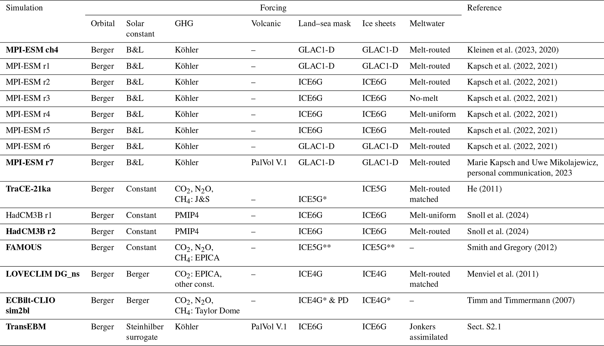
All 15 simulations are transient and cover at least the Last Deglaciation. We separate the simulations into a main set and a sensitivity set. Table 1 provides an overview of the simulations and forcing protocols. The following describes the ensemble in more detail:

• MPI-ESM ch4 (Kleinen et al., 2023, 2020)
  Model: This main set simulation used a setup of MPI-ESM v.1.2 at a coarse resolution called MPI-ESM-CR (Mauritsen et al., 2019; Mikolajewicz et al., 2018) with a methane cycle (Kleinen et al., 2020). Boundary conditions, including ice sheets, bathymetry, topography (Meccia and Mikolajewicz, 2018) from GLAC1-D (Briggs et al., 2014; Tarasov et al., 2012), and river routing (Riddick et al., 2018) were updated every 10 years. It covers 23 kyr BP until the present day.
  Simulated climate: This run simulates an LGM (23–19 kyr BP) to Holocene (8–0 kyr BP)³ warming of 4.4 °C and wetting of 0.27 mm d⁻¹. ⁴ At its start, it still cools in the global mean in tandem with an increase in the Equator-to-pole difference in the Southern Hemisphere and in sea ice volume (Fig. 2). It reaches its minimal GMST at around 21 kyr BP. The trend in increasing GMST during the Deglaciation is interrupted by abrupt decreases in GMST thrice: at around 14.5, 13.5, and 11.5 kyr BP. In comparison to other simulations, MPI-ESM ch4 simulates the smallest sea ice cover (Fig. 2c). Its global sea ice fraction is largest between 23 and 17 kyr BP and undergoes cycles of abrupt increase and decrease during the Deglaciation.

• MPI-ESM r1–r7 (Kapsch et al., 2022, 2021)
  Model: These seven simulations were produced using two more setups of MPI-ESM-CR. They also update boundary conditions every 10 years and cover the period from 26 kyr BP to the present day. They use different ice sheet reconstructions – GLAC1-D or ICE-6G_C (in the following ICE6G; Peltier et al., 2015) – and vary by meltwater scenario. Furthermore, a parameter for cloud formation was changed in r5–r7 to remove a cold bias found in r1–r4 (as detailed in the supporting information of Kapsch et al., 2022). The ice sheet reconstructions differ in their original resolution in time, with ICE6G providing updated boundary conditions at 500-year intervals and GLAC1-D at 100-year intervals, and were interpolated here to 10-year resolution. The meltwater scenarios follow the options outlined in the deglacial protocol of PMIP4 (Ivanovic et al., 2016): melt-uniform, melt-routed, and no-melt. These correspond to meltwater being distributed globally, through river-routing or being removed. Simulation r7 also applies a volcanic forcing by Schindlbeck-Belo et al. (2024) that builds on the Holocene reconstruction by Sigl et al. (2022), drawing on tephra records and including synthetic volcanic eruptions to mitigate underestimation of small eruptions. This simulation is part of the main set. Runs 1–6 form part of the sensitivity set. For two simulations, r3 and r4, only centennial means were available; thus they are only considered for the analysis of centennial variability.
  Simulated climate: These simulations exhibit the largest warming between the LGM and Holocene of the ensemble with a range from 5.3 °C (for r5) up to 6.6 °C (for r7; Figs. 2a and S1a). The accompanying global mean wetting is also the largest in the ensemble, ranging between 0.30 mm d⁻¹ (r5) and 0.39 mm d⁻¹ (r1 and r7). Runs 1, 6, and 7 further simulate abrupt cooling periods during the Deglaciation with the same timing as in MPI-ESM ch4. These are the simulations that employ the GLAC1-D ice sheet reconstruction and corresponding meltwater forcing. The remaining runs show either continuous or sometimes abrupt warming during those periods. The sea ice cover in these simulations is generally larger than in MPI-ESM ch4 and shows a stronger decrease towards the Holocene.

• TraCE-21ka (He, 2011)
  Model: The TraCE-21ka simulation was performed with CCSM3 (Collins et al., 2006) and stretches from 22 kyr BP to 1990 CE. This main set simulation was designed to match proxy data of millennial events such as the Bølling–Allerød and Younger Dryas during the Deglaciation (He, 2011). As such, it applies meltwater forcings in the Northern and Southern hemispheres at various times throughout the Deglaciation to reproduce proxy records (denoted as melt-routed matched). Ice sheets are updated at intervals of 500 years based on a modified version of the ICE5G reconstruction (ICE5G*; He, 2011; Peltier, 2004). As greenhouse gas forcing, TraCE-21ka uses Joos and Spahni (2008) (referred to as J&S in Table 1) with the age model of Monnin et al. (2001).
  Simulated climate: Among all simulations, TraCE-21ka tends towards the lower end of GMST and GMP change from the LGM to the Holocene at 4.1 °C and 0.20 mm d⁻¹. It shows abrupt warming around the time of the Bølling–Allerød interstadial (about 14.7–12.9 kyr BP) with subsequent cooling matching the Younger Dryas (circa 12.9–11.7 kyr BP; Fig. 2a). For most of the time period covered, TraCE-21ka produces the largest sea ice cover, with the exception of the EBM (Fig. 2c). This difference becomes particularly large towards the end of the Deglaciation and remains so throughout the Holocene.

• HadCM3B r1 & r2 (Snoll et al., 2024)
  Model: The ensemble contains two simulations from HadCM3B (Valdes et al., 2017) that cover 23 kyr BP to 2 kyr AP. These employ two different meltwater protocols, melt-uniform (r1) and melt-routed (r2), from the PMIP4 protocol to match the ICE6G ice sheet history. The simulations prescribe orbit and greenhouse gases (GHGs) annually, while ICE6G ice sheet, orography, land–sea mask, and bathymetry are updated every 500 years. HadCM3B r1 is part of the sensitivity set, while r2 is included in the main set.
  Simulated climate: The GMST difference between the LGM and the Holocene is 4.5 °C for the melt-uniform r1 and 4.8 °C for the melt-routed r2. Similarly, wetting of r1 is weaker at 0.26 mm d⁻¹ in comparison to 0.27 mm d⁻¹ for r2. The changes in Equator-to-pole gradient are notably small, especially in the Northern Hemisphere (Fig. 2d, e). Sea ice cover shrinks until 14 kyr BP and remains roughly constant thereafter (Fig. 2c).

• FAMOUS (Smith and Gregory, 2012)
  Model: FAMOUS is a low-resolution, slightly simplified version of HadCM3 (Smith et al., 2008). It is sometimes classified as an EMIC (as in Valdes et al., 2017) or as a low-resolution GCM based on the complexity of its atmosphere model. The simulation used here as part of the main set was run with an acceleration factor of 10 for all forcings, allowing it to cover the last 120 kyr (Smith and Gregory, 2012). The simulation does not consider sea level change; that is, ice sheets are present only where there are no modern ocean grid points. Furthermore, the ICE5G reconstruction and topographic changes (Peltier, 2004) were only applied north of 40° N (ICE5G**). In particular, the Antarctic ice sheet remains unchanged (Smith and Gregory, 2012).
  Simulated climate: FAMOUS simulates the smallest global mean change for both surface temperature and precipitation among all simulations at 3.1 °C and 0.15 mm d⁻¹, respectively. Its simulated Equator-to-pole temperature differences are among the largest in the ensemble, but they decrease comparatively little from the LGM to the present day (Fig. 2d, e).

• LOVECLIM DG_ns (Menviel et al., 2011)
  Model: This version of the EMIC LOVECLIM couples the atmosphere model ECBilt (Opsteegh et al., 1998) to the ocean model CLIO (Campin and Goosse, 1999; Goosse et al., 1999; Goosse and Fichefet, 1999). LOVECLIM DG_ns used ECBilt-CLIO v.3 coupled to a dynamical vegetation model with a terrestrial carbon cycle (Menviel et al., 2011) and is included in the main set. It focuses on the Deglaciation, running from 18–6.2 kyr BP. Employed greenhouse forcing is based on reconstructions from EPICA (Lüthi et al., 2008; Monnin et al., 2001; Spahni et al., 2005) mapped onto the EDC3 age scale (Parrenin et al., 2007). Like TraCE-21ka, it includes meltwater pulses in the North Atlantic and Southern Ocean (melt-routed matched) to reproduce millennial-scale events in the North Atlantic (McManus et al., 2004) and Greenland (Alley, 2000) during this period (Menviel et al., 2011).
  Simulated climate: As a result of the employed meltwater pulses, there are a warming and a subsequent cooling event visible in the global mean around the times of the Bølling–Allerød and the Younger Dryas, respectively (Fig. 2a, b). This signal is very strong in the Northern Hemisphere, where LOVECLIM DG_ns exhibits a large reduction in Equator-to-pole temperature gradient alongside these abrupt changes (Fig. 2d). In the Southern Hemisphere, this decrease is more subdued (Fig. 2e). Overall, the simulation shows deglacial warming and wetting comparable to most of the other simulations (Fig. 2a, b).

• ECBilt-CLIO sim2bl (Timm and Timmermann, 2007)
  Model: The second ECBilt simulation included in the main set uses the same coupled ocean and atmosphere models and covers the period from 21–0 kyr BP (Timm and Timmermann, 2007). It contains no meltwater forcing. For the ice sheets and land–sea mask of the atmosphere model, it applies ICE4G with the East Siberian ice sheet removed (ICE4G*). For the ocean model, the same ice sheet is used but combined with a constant land–sea mask representing present-day conditions (ICE4G* & PD).
  Simulated climate: Its simulated mean changes are 3.9 °C and 0.25 mm d⁻¹. Like LOVECLIM DG_ns, it has deglacial warming and wetting comparable to most of the other simulations (Fig. 2a, b). In magnitude, changes in ECBilt-CLIO sim2bl resemble those in LOVECLIM DG_ns (Fig. 2). Their structure is quite different, though, as ECBilt-CLIO sim2bl variables all change in a step-like manner. The simulated sea ice cover is at the upper end of the ensemble at the beginning of the simulation (similarly to TraCE-21ka and MPI-ESM r7) and then, like MPI-ESM r7, reduces drastically towards the Holocene (Fig. 2c).

• TransEBM (Sect. S2.1 in the Supplement)
  Model: To represent the linear temperature response of the climate system to external forcing, we juxtapose a simulation from an extended version of the 2D energy balance model TransEBM (Ziegler and Rehfeld, 2021) with the other simulations and include it in the main set. Here, it has been extended to include freshwater and zonal volcanic forcing. The simulation covers the surface temperature evolution of the last 26 kyr, with ICE6G boundary conditions updated every 125 or 500 years. Sea ice extent was interpolated between the LGM and present-day states given by Zhuang et al. (2017). Meltwater forcing was assimilated based on the database of sea surface temperature records by Jonkers et al. (2020) (Jonkers assimilated; see Sect. S2.1). The simulation employs the same volcanic forcing as MPI-ESM r7. Sect. S2.1 describes the simulation in more detail.
  Simulated climate: TransEBM simulates a GMST difference between the LGM and the Holocene of 4.1 °C, which is at the lower end of the ensemble and comparable to that of TraCE-21ka. Changes in Equator-to-pole difference are similar in magnitude in both hemispheres, unlike most other simulations (Fig. 2d, e). Its sea ice cover is the largest and changes the most during the Deglaciation because EBM models sea ice as a surface type, which covers any given grid cell completely.

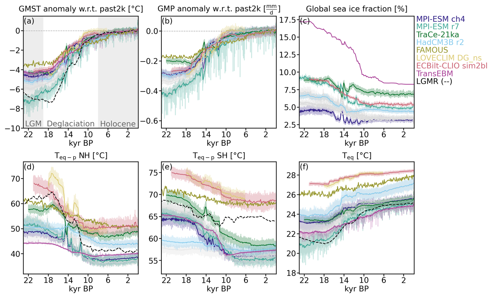
Figure 2 Centennial changes in the main set from the simulation ensemble from the LGM to the Holocene with annual data as shading. (a) GMST and (b) GMP anomaly with respect to the past 2 kyr. (c) Global sea ice fraction. Note that the EBM only allows complete coverage of grid cells by one surface type and therefore has the largest sea ice cover. FAMOUS and LOVECLIM DG_ns are missing, since their sea ice cover was not readily available. (d, e) Equator-to-pole temperature difference for the Northern Hemisphere and Southern Hemisphere, respectively, computed as the difference between polar (70–90°) and equatorial (15° S–15° N) temperatures. The latter are shown in panel (f). The sensitivity set is shown in gray and can be found in Fig. S1. LGM (23–19 kyr BP), Deglaciation (19–8 kyr BP), and Holocene (8–0 kyr BP) as used in this study are marked in panel (a).

Kleinen et al. (2023, 2020)Kapsch et al. (2022, 2021)Kapsch et al. (2022, 2021)Kapsch et al. (2022, 2021)Kapsch et al. (2022, 2021)Kapsch et al. (2022, 2021)Kapsch et al. (2022, 2021)He (2011)Snoll et al. (2024)Snoll et al. (2024)Smith and Gregory (2012)Menviel et al. (2011)Timm and Timmermann (2007)

Table 1 Forcings applied for the transient simulations of the Last Deglaciation. Further description in Sect. 2.1. Labels of main set simulations are bold.

To summarize, the main set is made up of MPI-ESM ch4 and r7, TraCE-21ka, HadCM3B r2, FAMOUS, LOVECLIM DG_ns, ECBilt-CLIO sim2bl, and TransEBM. MPI-ESM r1–r6 and HadCM3B r1 form the sensitivity set.

2.2 The model hierarchy

We construct a hierarchy of the models to summarize the outlined differences and thus understand their effects on all aspects of climate variability. The complexity of the models and simulations differs along several axes: resolution in time and space, complexity of the individual components (e.g., atmosphere, ocean, land surface), their coupling, and their forcing. Constructing a hierarchy of models or simulations helps summarize those differences and thus understand their effect on any given analysis. The relevant axes of comparison might differ between applications. As a consequence, ranking the same models and simulations might produce a different hierarchy depending on the application. Here, we establish a hierarchy focused on features that affect variability and for which the simulations meaningfully differ.

Based on these considerations, we include eight axes of comparison (Fig. 3a). Section S2.2 explores these axes and the classification of the simulations. The resulting hierarchy reveals the various levels of complexity of the different simulations by placing them along each axis. In general, a simulation is considered more complex, the larger the total area it covers. Whenever an axis of the hierarchy does not apply to a simulation, the rank will be at the center of the net; see the lack of dedicated ocean or land hydrology model in TransEBM.

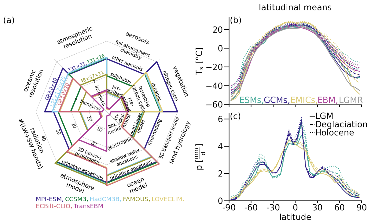
Figure 3 (a) Ranking of the models used in this study along eight axes of complexity. The criteria are described in detail in Sect. 2.2 and Table S1. Altogether they establish a hierarchy of the different models: ESMs (MPI-ESM), GCMs (CCSM3, HadCM3B, FAMOUS), EMICs (LOVECLIM, ECBilt-CLIO), and the EBM (TransEBM). Atmospheric and oceanic resolutions of some of the simulations are listed, with the vertical resolution always last. (b, c) Latitudinal distributions of mean temperature and precipitation for hierarchy categories based on panel (a). For temperature, the biggest spread between the models and largest overall increases from the LGM to the Holocene can be found in the polar regions. For precipitation, the simulations and periods vary most in the tropics and the mid-latitude bands.

Based on all the factors summarized in Fig. 3a, we separate all simulations into four groups of complexity for parts of our analysis: ESMs (MPI-ESM), GCMs (TraCE-21ka, HadCM3B1, FAMOUS), EMICs (LOVECLIM, ECBilt-CLIO), and the EBM (TransEBM). The categorization follows the overall number of levels reached in the hierarchy. In the end, both applied forcings and complexity of the model components decide the simulation output. Our analysis tries to identify and disentangle the effects of both on simulated variability, with the goal of identifying the complexity both necessary and sufficient for long, transient climate simulations. Since increased complexity implies higher computational demand, a trade-off has to be made between complexity and available resources. Knowing the benefits and limitations of added complexity is thus crucial.

2.3 Global climate reanalysis data

For quantitative comparison, we draw on a spatiotemporally gridded product, the LGM reanalysis LGMR by Osman et al. (2021), which covers the past 24 000 years. LGMR combines model simulations and proxy reconstructions in an offline data assimilation approach for a proxy-constrained estimate of the full field of surface temperature since the LGM. The resulting dataset has a resolution in time of 200 years, allowing a comparison of centennial variability to the results of our analysis. The reanalysis relies on model priors from 17 time-slice experiments from iCESM1 (Brady et al., 2019) and 539 geochemical proxy records of sea surface temperature. Using a Bayesian forward model, proxy values are estimated for given time steps at every proxy location from the model prior. This produces a forward-modeled proxy value different from the actual proxy value. To take uncertainties and the covariance between proxy location and the climate field into account, this difference is weighted by the Kalman gain for the update of the model prior temperature field. The resulting reanalysis estimates a global warming of 7.0±1.0 °C from the end of the LGM to the PI (with PI defined as 1000–1850 CE), as it is contains an LGM state colder than reconstructed elsewhere (cf. Annan et al., 2022; Tierney et al., 2020; Shakun and Carlson, 2010). However, unlike other reconstructions, LGMR provides a gridded reconstruction of the surface temperature field covering the whole time period of interest here, not just the LGM. Here, we use the ensemble mean as the basis for our calculations of variability.

3 Methods

Climate can be represented by sets of observations in space and time. The field of a climate variable then refers to usually gridded spatial representations of that variable (von Storch and Zwiers, 1999). Conversely, a time series specifies the sequence of observations in time (Chatfield, 2016). As such, climate variables can be treated as random variables with associated probability distributions, and time series represent realizations of a stochastic process. Here, we analyze the statistical properties of the time series of surface temperature and precipitation in space and time by computing their moments and power spectra.

In order to compare the transient simulations, we first re-grid them to a common T21 resolution, which is the lowest commonly used resolution in the ensemble. We further compute decadal and centennial means of the annual data to obtain the variability on those timescales. Then, we extract the time periods, LGM (23–19 kyr BP), Deglaciation (19–8 kyr BP), and Holocene (8–0 kyr BP), from all time series (see Fig. 2a). Finally, we remove the trend from the time series using a Gaussian filter with a kernel length equivalent to 4000 years,⁵ which is the length of the LGM as the shortest time period we investigate. After detrending, we can assume that the resulting time series are (weakly) stationary, a requirement for the estimation of moments, along with the autocovariance function and thus the spectrum.

3.1 Moments of a probability distribution

The distributions of surface temperature and precipitation cannot be assumed to be normal. Precipitation in particular often has heavier tails than a normal distribution (Franzke et al., 2020). To describe the shape of the distributions of climate variables, we turn to the four moments: mean, standard deviation, skewness, and kurtosis (Fig. 4; von Storch and Zwiers, 1999). We compute them for every grid box and time period. These are then area-averaged globally or zonally when providing the respective means of the moments.

Figure 4 Visualization of changes in the moments of the distribution of a random variable, with individual changes on top and concurrent changes on the bottom. Distributions for a lower (pink) and higher (green) value are shown. Panels (a)–(d) show changes in just one moment: (a) mean, (b) variance, (c) skewness, and (d) excess kurtosis. Panels (e)–(h) show exemplary combinations of changes in the higher moments with constant mean: (e) opposite changes in variance and skewness, (f) concurrent change in variance and kurtosis, (g) concurrent change in skewness and kurtosis, and (h) changes in all higher moments. Figure S4 shows exemplary time series corresponding to the distributions.

The generalized moments of random variable X of a point A for a sample of size N are defined using the expected value as

$$\begin{array}{}\text{(1)}& {\mathit{\mu }}_n=\mathbb{E}\left[\right(X-A{)}^n]={\displaystyle \frac{\mathrm{1}}{N}}\sum _{i=\mathrm{1}}^N(X_i-A{)}^n,\end{array}$$

where n designates the nth moment (Papoulis and Pillai, 2002). There exist variations of this definition of the moments depending on normalization or bias correction terms. We introduce them in more detail in Sect. S3.1. Here, we focus on the definitions used in the analysis. To assess the background climate state, we use the arithmetic mean μ for n=1 (Fig. 4a; Papoulis and Pillai, 2002) and the expected values computed about the origin, such that

$$\begin{array}{}\text{(2)}& {\mathit{\mu }}_{\mathrm{1}}\equiv \mathit{\mu }=\mathbb{E}\left[X\right]={\displaystyle \frac{\mathrm{1}}{N}}\sum _{i=\mathrm{1}}^N{X}_i.\end{array}$$

Considering the moments about the mean μ instead yields

$$\begin{array}{}\text{(3)}& m_n={\displaystyle \frac{\mathrm{1}}{N}}\sum _{i=\mathrm{1}}^N(X_i-\mathit{\mu }{)}^n,\end{array}$$

called nth central moment (Papoulis and Pillai, 2002; von Storch and Zwiers, 1999). For the second moment, variance, we use a symmetric unbiased estimator (Filliben and Heckert, 2024), yielding

$$\begin{array}{}\text{(4)}& {\mathit{\sigma }}^{\mathrm{2}}={\displaystyle \frac{N}{N-\mathrm{1}}}{m}_{\mathrm{2}}={\displaystyle \frac{\mathrm{1}}{N-\mathrm{1}}}\sum _{i=\mathrm{1}}^N(X_i-\mathit{\mu }{)}^{\mathrm{2}}.\end{array}$$

It describes the spread of the distribution – the larger the variance and its square root standard deviation σ, the larger the spread around mean μ (Fig. 4b).

For the third moment, skewness (s), we use

$$\begin{array}{}\text{(5)}& s={\displaystyle \frac{m_{\mathrm{3}}}{m_{\mathrm{2}}^{\mathrm{3}/\mathrm{2}}}}.\end{array}$$

Skewness describes the (a)symmetry of a distribution (von Storch and Zwiers, 1999). It is zero for a symmetric distribution, e.g., for the normal distribution. For negative skewness, the weight of the distribution is at higher values, with mode and median larger than the mean (Fig. 4c). This implies a stronger tail for lower than higher values: the distribution is “skewed left”. For positive skewness, on the other hand, mode and median are smaller than the mean: the distribution is skewed towards higher values. To test whether any skewness found differs significantly from a normal distribution, we test its deviation from normality for significance using a t-test. For this test, the null hypothesis is that the skewness found and that of a corresponding normal distribution are the same and thus 0. We define the threshold for the p-value to be 0.05.

Adapting the skewness definition for n=4, kurtosis, yields a kurtosis of 3 for a normal distribution. To derive an estimator which is 0 for normal distributions, kurtosis is often shifted by −3 to derive excess kurtosis k (Filliben and Heckert, 2024). Based on the fourth and second central moment, we calculate excess kurtosis as

$$\begin{array}{}\text{(6)}& k={\displaystyle \frac{m_{\mathrm{4}}}{m_{\mathrm{2}}^{\mathrm{2}}}}-\mathrm{3}.\end{array}$$

We use excess kurtosis throughout the paper; for the sake of brevity, we will refer to it as kurtosis from now on. Kurtosis captures the heaviness of the tails of a distribution (Fig. 4d). If excess kurtosis is negative, the tails are thinner than those of a normal distribution. Conversely, positive excess kurtosis corresponds to heavier tails. Generally, positive kurtosis and skewness co-occur for datasets with more extreme values (Doane and Seward, 2011). As for skewness, we check again for non-normality using the hypothesis test derived by Anscombe and Glynn (1983) with a threshold for the p-value of 0.05. For all computations, we ignore rare not-a-number (nan) values in the temperature or precipitation fields. Changes in moments often occur concurrently and can then both enhance or counteract each other (Fig. 4).

3.2 Spectral analysis

In order to analyze how the variability in surface temperature and precipitation depends on timescale, we further compute the power spectral density (PSD), also called the power spectrum. If a process contains (quasi-)oscillatory components, the spectrum shows a peak at their periodicity with a certain width related to the damping rate of that process. The spectrum's background and scaling reflect the persistence (or memory) of the process (Ditlevsen et al., 2020).

The auto-covariance function for a random variable X_t at times t₁ and t₂ is given by the expectation value of its variance as

$$\begin{array}{}\text{(7)}& \mathit{\gamma }(t_{\mathrm{1}},t_{\mathrm{2}})=\mathbb{E}\left[\right(X\left(t_{\mathrm{1}}\right)-\mathit{\mu }\left(t_{\mathrm{1}}\right)\left)\right(X\left(t_{\mathrm{2}}\right)-\mathit{\mu }\left(t_{\mathrm{2}}\right)\left)\right],\end{array}$$

where γ(0)=𝔼[X²] is the variance.

If the time series samples an ergodic, weakly stationary stochastic process, the auto-covariance and mean are independent of time and thus depend only on lag, $\mathit{\tau }=t_{\mathrm{2}}-t_{\mathrm{1}}$. Assuming further that the data X_T are an excerpt of a theoretically infinite time series such that they are non-zero only for an interval $t\in [-\frac{T}{\mathrm{2}},\frac{T}{\mathrm{2}}]$ (Ditlevsen et al., 2020), auto-covariance can be written as

$$\begin{array}{}\text{(8)}& {\displaystyle }\mathit{\gamma }\left(\mathit{\tau }\right)=\mathbb{E}\left(\right(X\left(t\right)-\mathit{\mu }\left)\right(X(t+\mathit{\tau })-\mathit{\mu }\left)\right),\text{(9)}& {\displaystyle }=\underset{T\to \mathrm{\infty }}{lim}{\displaystyle \frac{\mathrm{1}}{T}}\underset{-T/\mathrm{2}}{\overset{T/\mathrm{2}}{\int }}X\left(t\right)X(t+\mathit{\tau })\mathrm{d}t.\end{array}$$

The PSD S for frequency ω is then defined as the Fourier transform ℱ of the autocovariance

$$\begin{array}{}\text{(10)}& {\displaystyle }S\left(\mathit{\omega }\right)=\mathcal{F}\left(\mathit{\gamma }\right(\mathit{\tau }\left)\right)\left(\mathit{\omega }\right),\text{(11)}& {\displaystyle }=\underset{-T/\mathrm{2}}{\overset{T/\mathrm{2}}{\int }}\mathit{\gamma }\left(\mathit{\tau }\right){\exp }^{-i\mathit{\omega }\mathit{\tau }}\mathrm{d}\mathit{\tau }.\end{array}$$

The spectra of climate variables sometimes scale consistently across timescales following a power law with $S\left(\mathit{\omega }\right)\propto {\mathit{\omega }}^{-\mathit{\beta }}$, with β as the so-called scaling coefficient (Fredriksen and Rypdal, 2017; Lovejoy and Varotsos, 2016; Huybers and Curry, 2006; Wunsch, 2003). The scaling coefficient then reflects the persistence of the stochastic process.

To estimate PSDs, we apply the multi-taper method (Thomson, 1982; Percival and Walden, 1993) to the detrended time series. For data of finite length, this method reduces spectral leakage by computing separate spectra for orthogonal windows, so-called tapers, and averages the resulting spectra. Here, we use three tapers and estimate chi-squared distributed confidence intervals. We smooth the resulting spectrum and cut off artifacts at the low- and high-frequency end, such that, for a time series with a time step t_s, a period range of [2t_s,1000] remains. For comparing the variance in the different time periods across timescales, we further compute the spectral gain following Ellerhoff and Rehfeld (2021) by dividing the spectrum of the LGM and Deglaciation, respectively, by that of the Holocene.

4 Results

We examine changes in variability against a backdrop of a changing mean state, which we examine first (Sect. 4.1). Then, we evaluate temperature moments with respect to their dependence on mean state (LGM, Deglaciation, and Holocene), timescale, and model complexity (Sect. 4.2). Next, we focus on the forcing dependency by analyzing the influence of ice sheet reconstruction (Sect. 4.3.1), meltwater protocol (Sect. 4.3.2), and volcanism (Sect. 4.3.3) on surface temperature variability. Sections 4.4 and 4.5 repeat the analysis for precipitation. Then, we turn to the power spectra of temperature and precipitation, again considering state and forcing dependency, as well as differences related to model complexity (Sect. 4.6). We further compare the temperature spectra to results from the LGM reanalysis.

4.1 Mean state changes from LGM to Holocene across the ensemble

Between the LGM and the Holocene, all simulations show a mean warming and wetting, as evidenced by the increasing trends in GMST and GMP towards the Holocene (Fig. 2). Overall, MPI-ESM r1–r7 exhibit the largest temperature difference between the LGM and the Holocene with an average increase of 5.6 °C. Among the simulations, the anomaly is largest and the simulated LGM temperature is lowest for the simulations with GLAC1-D as the ice sheet reconstruction. In the whole ensemble, LGM cooling is widespread and especially pronounced in the high latitudes on land, with the exception of a few localized hotspots in a few of the simulations, e.g., an Alaskan warm patch in TraCE-21ka (Fig. S8g, h). Inter-simulation differences are generally larger in the high latitudes, especially in the Northern Hemisphere (Fig. 3b). For precipitation, the picture is more diverse, but, in most places and especially over land, a drier LGM is simulated. Some simulations show a locally wetter LGM in the tropics, a phenomenon mostly confined to the oceans. ESMs and GCMs show similar latitudinal profiles, while the EMICs miss some precipitation in the inner tropics and mid-latitude westerlies (Fig. 3c).

4.2 State and timescale dependency of surface temperature

Analyzing the higher-order moments of surface temperature reveals their dependence on timescale and model complexity (Figs. 5, S5). The standard deviation of surface temperature and its regional differences decrease towards longer timescales (Fig. 5a, d, g). Most of this decrease occurs between annual and decadal timescales. The only exception to this pattern is the EBM, which has low standard deviation across all periods. Differences between the three periods in the ensemble are concentrated in higher latitudes, especially in the northern polar regions. On annual scales, the Holocene standard deviation is smaller there than during the LGM and Deglaciation, which are similar to each other. For decadal and centennial scales, on the other hand, the Deglaciation stands out with higher standard deviation, while the Holocene and the LGM exhibit more similar levels. The LGMR shows similar patterns on centennial scales.

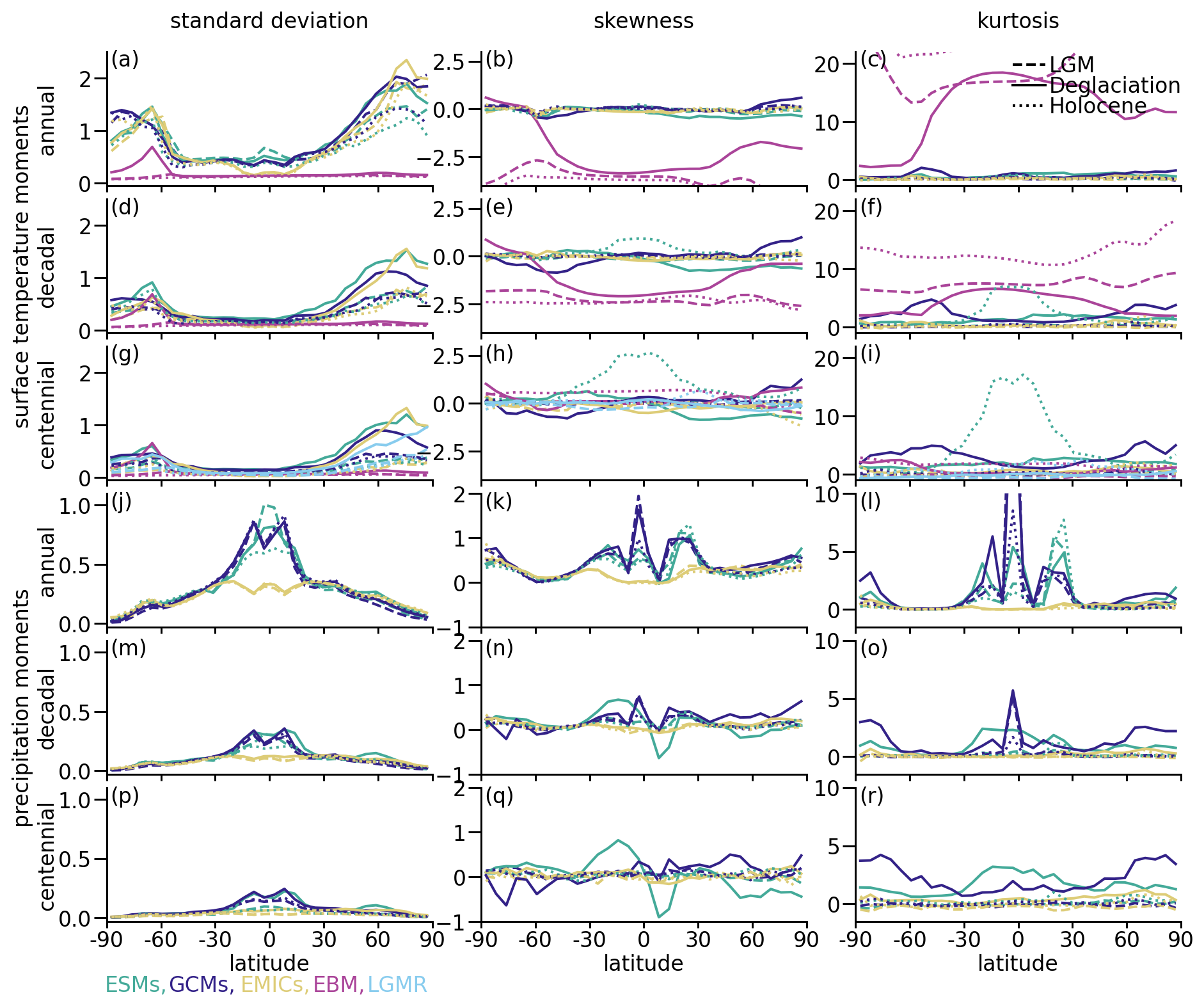
Figure 5 Changes of annual, decadal, and centennial higher-order moments of surface temperature (a–i) and precipitation (j–r) with latitude. For all simulations, standard deviation (left column, in units of °C for temperature and mm d⁻¹ for precipitation), skewness (middle column, dimensionless), and kurtosis (right column, dimensionless) are shown. Results are differentiated according to period (LGM (dashed), Deglaciation (solid), and Holocene (dotted)) and complexity (ESMs (green), GCMs (dark blue), EMICs (yellow), and EBM (pink)). For centennial temperatures, moments of the LGMR ensemble mean are added in light blue. For temperature, the range of skewness and kurtosis of the EBM extend beyond what is shown, as does the kurtosis in HadCM3B for precipitation. Figures S6 and S7 show the individual simulations.

As a measure of asymmetry, skewness is positive (negative) if the weight of the distribution is at lower (higher) values with a high (low) value tail (see Sect. 3.1). Globally and across latitudes, skewness of temperature is usually close to zero, indicating little asymmetry (Figs. 5b, e, h, S5). The EBM is the exception as it shows pronounced negative skew, a signal that shrinks towards longer timescales. On centennial scales, the lack of skewness in the ensemble agrees with the results for the LGMR ensemble mean. In certain latitudinal bands, more significant deviations from zero exist. For example, MPI-ESM r1–6 and TraCE-21ka show positive centennial and, to a lesser degree, decadal skewness in the tropics during the Holocene, in particular over the ocean. This signal disappears with the addition of volcanic forcing in MPI-ESM r7 (Fig. 5h). In the MPI-ESM simulations, it is not reflective of physical processes in the climate system (Ellerhoff and Rehfeld, 2021). Therefore, we exclude it in the discussion of skewness and kurtosis going forward. Furthermore, TraCE-21ka shows a strong bipolar pattern during the Deglaciation on all timescales, with negative skewness in the Southern Hemisphere and positive skewness in the Northern Hemisphere (Figs. 5h and S9n). All other simulations show either no hemispheric pattern or, in the case of some MPI-ESM simulations and, to a lesser degree, HadCM3B, the opposite one, although with smaller magnitudes (Figs. 5h and S9k). For the MPI-ESM simulations, this bipolar pattern mostly shows up in the runs employing the GLAC1-D ice sheet (ch4, r1, r6, r7). The pattern is weaker for the melt-uniform runs (MPI-ESM r4 and HadCM3B r1) and disappears without meltwater forcing (MPI-ESM r3 and HadCM3B r2).

Kurtosis reflects the heaviness of the tails, defined here such that positive (negative) kurtosis corresponds to tails more (less) pronounced than those of the normal distribution (see Sect. 3.1). As for skewness, the kurtosis is mostly small on annual timescales, across periods and simulations in the ensemble and LGMR (Figs. 5c, S5c). Towards longer timescales, some regional differences emerge (Figs. 5f, i, S5f, i). TraCE-21ka again deviates during the Deglaciation, with temperatures that show strong positive kurtosis that is strongest in the high latitudes (Figs. S6o, r, and S9w). The EBM behaves differently on annual and decadal scales, simulating a strong positive kurtosis and thus heavy tails. On centennial scales, the EBM is again close to the more complex models.

4.3 Influence of forcings on the moments of surface temperature distributions

Using the sensitivity set, we investigate the interaction between forcings and moments of temperature distributions, in particular regarding the underlying ice sheet reconstruction (Sect. 4.3.1), meltwater protocol (Sect. 4.3.2), and volcanic forcing (Sect. 4.3.3).

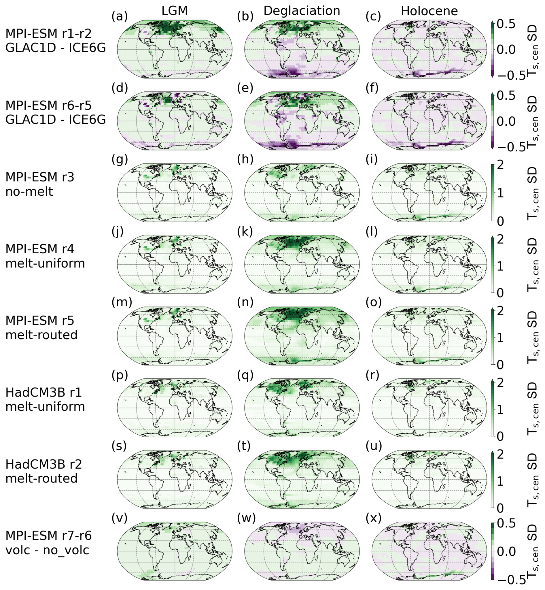
Figure 6 Regional effects of forcings on centennial standard deviation of surface temperature. (a–f) Influence of ice sheet forcing as differences between MPI-ESM runs using GLAC1-D and ICE6G. (g–u) MPI-ESM (g–o) and HadCM3B (p–u) simulations following different meltwater protocols. (v–x) Difference between MPI-ESM r7 with volcanic forcing and r6 without it.

4.3.1 Effect of ice sheet reconstructions on the shape of surface temperature distributions

Changes in standard deviation are regionally limited in response to the prescribed ice sheet reconstruction (Fig. 6a–f). On centennial timescales, ICE6G runs simulate smaller standard deviation in the northern North Atlantic compared to the runs using GLAC1-D (cf. MPI-ESM r1 and r6; Fig. 6a, b, d, e). This coincides with a reduced sea ice cover in these runs and a smaller temperature difference between the LGM and Holocene (Fig. S1a and c). The opposite pattern occurs in areas of Antarctic sea ice, especially the Weddell Sea, where ICE6G runs have higher standard deviation (Fig. 6b, e).

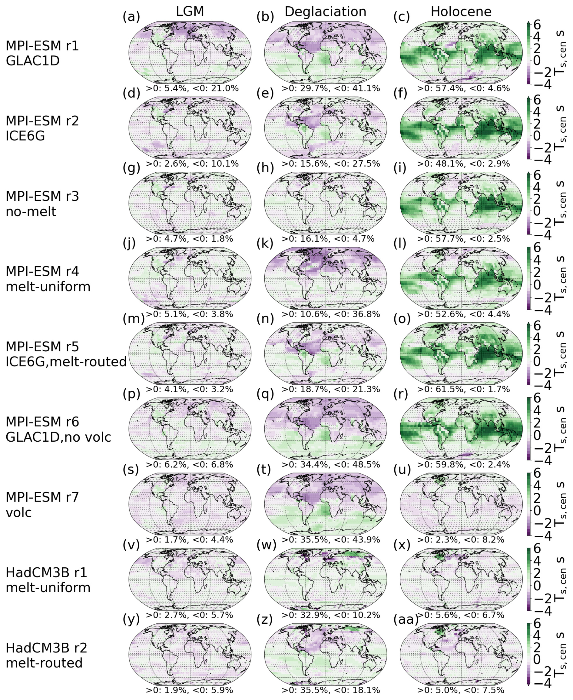
Figure 7 Regional effects of forcings on centennial skewness of surface temperature. Forcings are noted along with the run name for each row. Percentages of grid boxes with significant positive and negative deviations from a Gaussian distribution are given. Areas where changes are non-significant are hatched.

On centennial timescales, more areas in the simulations using GLAC1-D tend to have significant skewness, both positive and negative, than in simulations using ICE6G (Fig. 7). During the Deglaciation, the bipolar pattern of negative skewness in the Northern Hemisphere and positive skew in the Southern Hemisphere that emerges on decadal and centennial timescales is enhanced in the GLAC1-D simulations (Figs. 7, S13). On decadal and annual scales, the simulations with ICE6G can, at times, show opposite trends in comparison to their respective GLAC1-D simulations (Figs. S13, S14). The chosen ice sheet reconstruction has a limited impact on temperature kurtosis on annual to centennial timescales (Figs. 8, S15, S16).

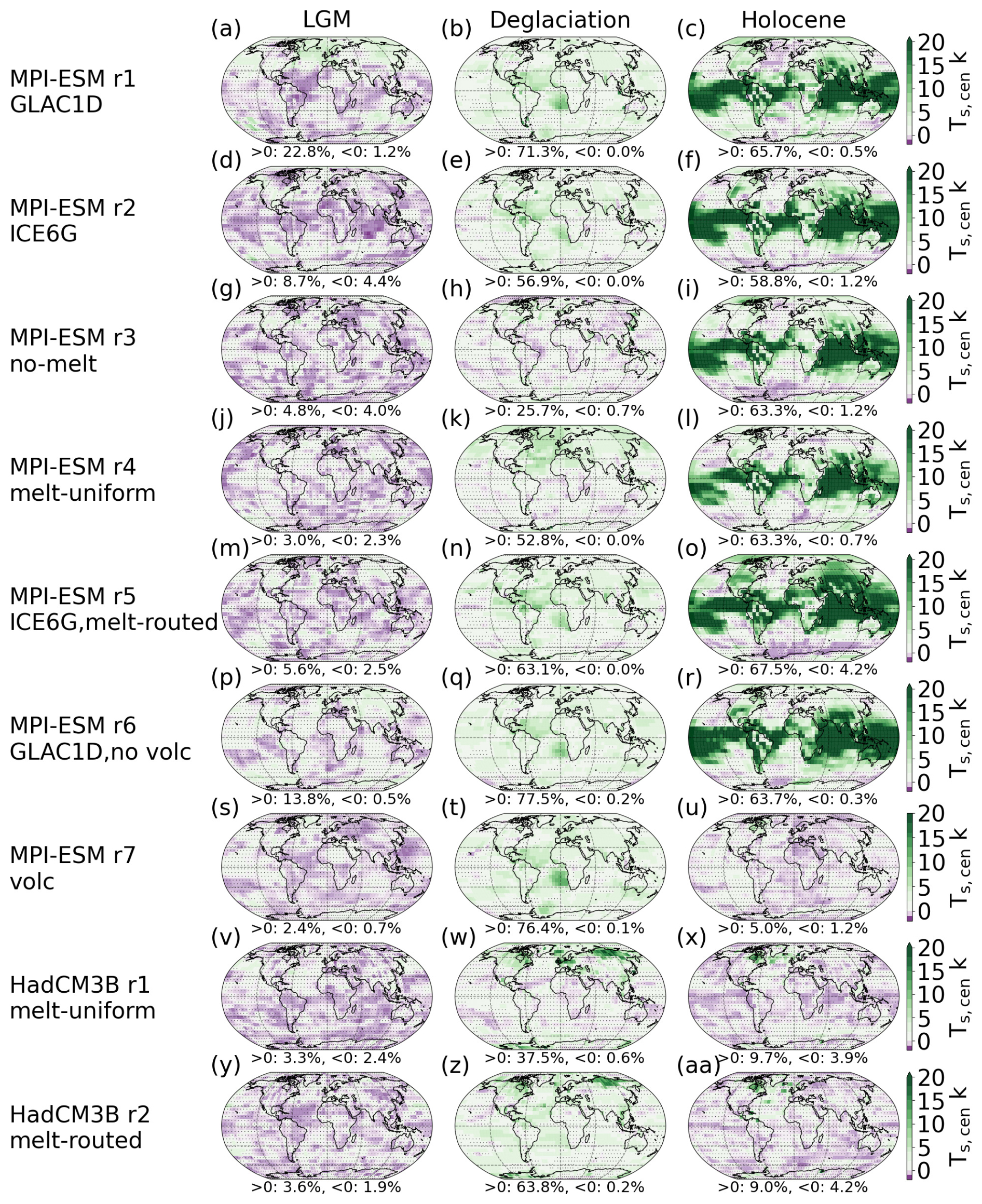
Figure 8 Regional effects of forcings on centennial kurtosis of surface temperature. Forcings are noted along with the run name for each row. Percentages of grid boxes with significant positive and negative deviations from a Gaussian distribution are given. Areas where changes are non-significant are hatched.

4.3.2 Effect of meltwater protocols on surface temperature distributions

Meltwater forcing affects the moments particularly during the Deglaciation and in the North Atlantic (Figs. 6, 7, 8). The local melt-routed protocol is associated with the largest moments, and the no-melt scenario is associated with the smallest moments. This holds in particular in the North Atlantic. Furthermore, the melt-routed simulation has the strongest signal in the Southern Ocean.

For skewness, the North Atlantic is associated with a negative signal, again strongest for the melt-routed scenario (Fig. 7). The melt-routed runs further show positive skewness in the southern Atlantic and the southeastern Pacific. On the other hand, the uniform runs do not show consistent patterns: MPI-ESM r4 simulates negative skewness over large parts of the middle and high latitudes in the Northern Hemisphere, whereas HadCM3B r1 only has significant, mostly positive, skewness in a few regions (Fig. 7). The absence of meltwater forcing, as in MPI-ESM r3, results in a notable lack of significant skewness across the globe. Across the ensemble, including meltwater mostly introduces a shift to more positive kurtosis during the Deglaciation, especially in the North Atlantic (Fig. 8). This positive shift is stronger in the melt-routed (HadCM3B r2, MPI-ESM r2) than in the melt-uniform simulations (HadCM3B r1, MPI-ESM r4) on all timescales, although to varying degrees.

4.3.3 Effect of volcanism on surface temperature distributions

For standard deviation of temperature, the effects of volcanism are mostly limited to shorter timescales but are overall small (Figs. 6v–x, S12). During the LGM, the run with volcanic forcing has a higher standard deviation than the one without. For the Deglaciation and Holocene, volcanism results in standard deviation that is greater at lower latitudes but smaller at higher latitudes.

Generally, volcanism results in negatively skewed temperature distributions or a reduction in positive skew, since it lowers temperatures after eruptions (Fig. S14j–o). It has the strongest effect on shorter timescales and during the LGM and Holocene. For the LGM, volcanic activity introduces a pronounced negative signal, mostly confined to the tropics. During the Holocene, skewness is decreased as well, turning the unphysical positive signal over the tropics (see Sect. 4.2 and Ellerhoff and Rehfeld, 2021) and most land areas into slightly negative skewness in parts of the tropics and effectively zero elsewhere (Fig. S15). On centennial scales, volcanic activity mainly manifests in skewness during the Holocene, where it again counteracts strong positive skewness in the tropics (Fig. 7r, u).

In contrast to ice sheet and meltwater forcings, volcanic forcing impacts kurtosis on all timescales and for all periods (Figs. 8p–u, S15j–o, S16j–o). For annual temperatures, it shifts the kurtosis to be positive in extended areas, particularly in the tropics and at northern mid-latitudes. This effect persists on decadal and centennial timescales for the LGM and Deglaciation. During the Holocene and on longer timescales, on the other hand, it reduces the low and mid-latitude band of positive kurtosis in the tropics. With volcanism, skewness and kurtosis in MPI-ESM r7 resemble HadCM3B r2 on centennial scales (Figs. 7, 8). On annual scales, however, volcanic forcing introduces skewness and kurtosis patterns unlike any other simulation (Figs. S14, S16).

4.4 State dependency of precipitation at annual to centennial timescales

The standard deviation of precipitation is high in the tropics and decreases towards higher latitudes (Fig. 5). In particular, it is high over the tropical oceans in the region of the intertropical convergence zone (ITCZ; Figs. 5j and S11a–i), where mean precipitation is also highest (Fig. 3c). The tropical band of increased standard deviation exists only to a lesser degree in the EMIC simulations (Fig. S6). State dependency exists on centennial but only very rarely on annual timescales. During the Deglaciation, the tropical pattern of enhanced standard deviation remains on centennial scales but is less pronounced than on annual scales. The spatial patterns of the LGM and Holocene, on the other hand, are more homogeneous, and the tropical standard deviation is similar to that at other latitudes (Fig. 9). The only exception is the FAMOUS simulation, which has enhanced tropical standard deviation for all three periods and the overall largest magnitudes in the ensemble on centennial scales (Fig. S6p).

The higher moments show more diverse patterns for precipitation (Figs. 5, S5). For skewness, the simulations mostly show positive precipitation skewness on annual scales, with some negative skewness in areas near the Equator and little difference between the periods (Fig. S11). The tropics also show the largest positive skewness. The EMICs simulate the smallest skewness, although the positive deviation from zero is still significant almost everywhere (Figs. 5, S11). The ESMs and GCMs, on the other hand, simulate very similar patterns on annual scales. Starting on decadal and even more strongly on centennial scales, the patterns diverge between periods and simulations (Figs. 5q, S10j–r). During the LGM and Holocene, centennial skewness is close to zero and thus indicates predominantly symmetric distributions. During the Deglaciation, skewness patterns are far more diverse, with a larger spread and including negative excursions. These center mostly around the Equator but also sometimes in the high northern (for MPI-ESM simulations with a GLAC1-D ice sheet; Fig. 10) or the high southern latitudes (for TraCE-21ka; Fig. S10n). In a bipolar pattern, TraCE-21ka further simulates high positive skewness in the high northern latitudes (Figs. S6n, q and S10n). The EMICs and FAMOUS show almost no significant skew in all periods on decadal and centennial scales (Fig. S6).

Precipitation kurtosis is mostly positive on annual scales across the periods in ESM and GCM simulations, in particular in the tropical regions (Figs. 5, S5, S11). The LGM and Holocene exhibit no significant kurtosis on longer timescales. During the Deglaciation, though, positive kurtosis persists. The EMICs, on the other hand, have some significant kurtosis only during the Deglaciation on annual scales and otherwise show no significant deviation from zero in contrast to the more complex models.

4.5 Changes in precipitation distribution shape in response to forcings

For the moments of precipitation, forcing dependency can mostly be found for meltwater forcing (Figs. 9, 10). Effects of the ice sheet reconstructions are mostly limited to centennial skewness in the tropics, in the North Atlantic zone, and in mid- and high latitudes in Eurasia (Fig. 10). These are the very same areas where temperature skewness changes the most. The skewness patterns in the tropics agree between the reconstructions but are enhanced in the GLAC1-D simulations. An exception is the high northern latitudes during the Deglaciation, where skewness is positive in the ICE6G simulations and negative in the GLAC1-D ones (Fig. 10).

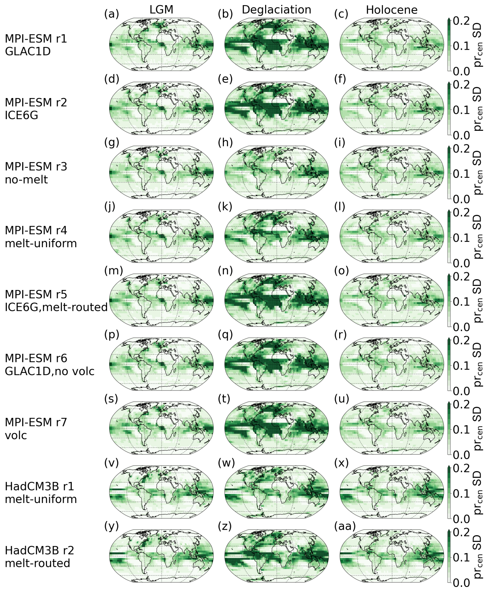
Figure 9 Regional effects of forcings on centennial standard deviation of precipitation. Forcings are noted along with the run name for each row.

Meltwater forcing affects all Deglacial moments, in particular in the tropics and North Atlantic. Standard deviation is largest in the melt-routed runs (MPI-ESM r2 and HadCM3B r2) and smallest in the no-melt simulation (Fig. 9). Injecting meltwater introduces significant skewness in precipitation distributions during the Deglaciation on centennial timescales (Fig. 10). Both melt-routed simulations (MPI-ESM r5 and HadCM3B r2) have a signal of negative skewness in the eastern equatorial Pacific, with a positive signal to the south of it. Only the positive signal remains somewhat in the melt-uniform runs. These MPI-ESM and HadCM3B runs further exhibit strong negative skewness in high northern latitudes, although in different areas. The influence of meltwater forcing on centennial kurtosis during the Deglaciation shows up predominantly as positive kurtosis (Fig. S7). Melt-routed runs have more positive kurtosis in the tropics, whereas melt-uniform simulations have more in the high northern latitudes. Overall, ice sheet reconstruction, meltwater protocol, and volcanic forcing (see annual moments in Figs. S17, S18) usually affect the moments of temperature more than those of precipitation.

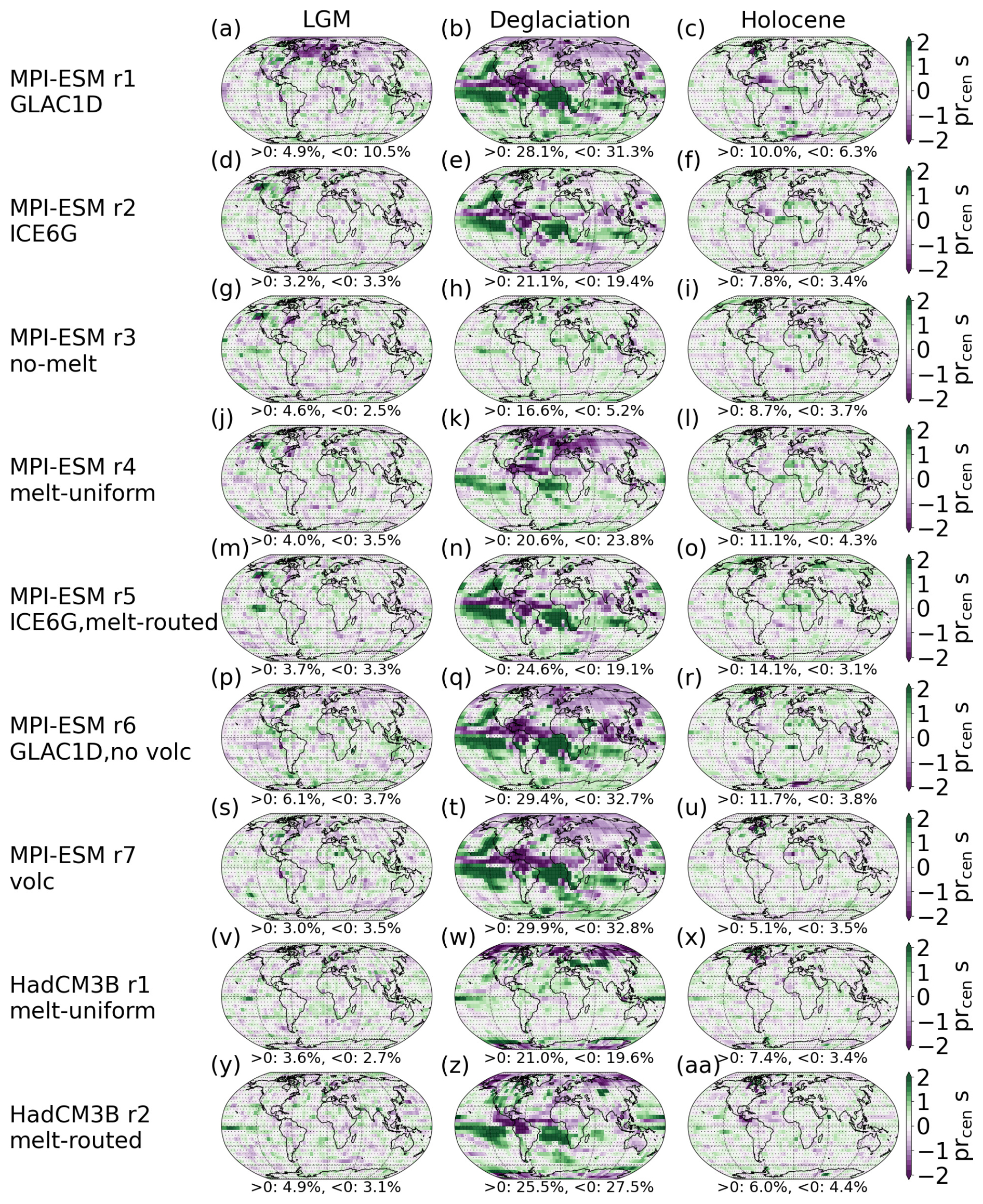
Figure 10 Regional effects of forcings on centennial skewness of precipitation. Forcings are noted along with the run name for each row. Percentages of grid boxes with significant positive and negative deviations from a Gaussian distribution are given. Areas where changes are non-significant are hatched.

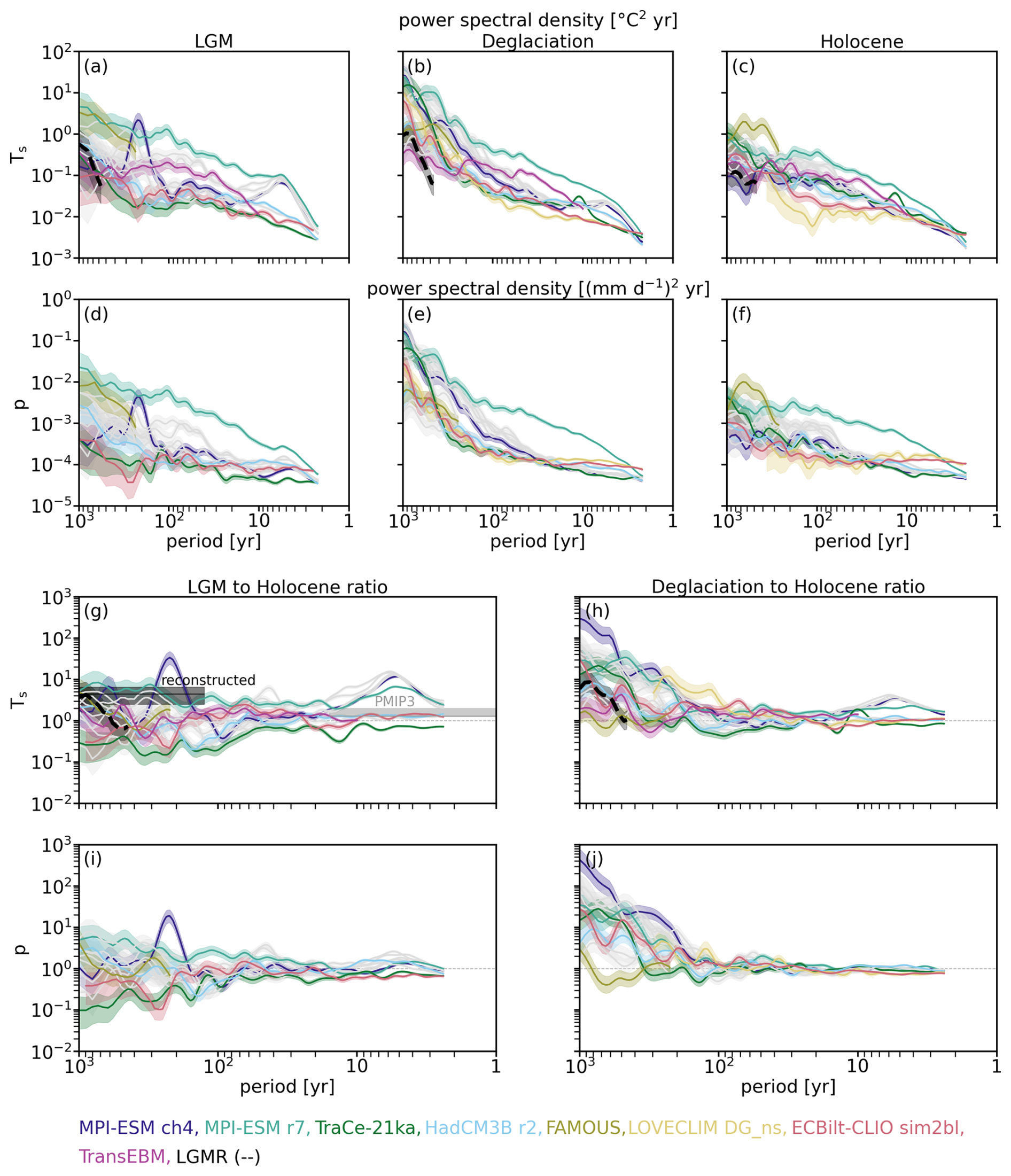
Figure 11 Spectra and spectral ratios of surface temperature (top row) and precipitation (bottom row) variability with chi-squared distributed confidence intervals. Both the x and the y axis are shown on a logarithmic scale. The spectra are separated by time period: (a, f) LGM, (b, g) Deglaciation, and (c, h) Holocene. The spectral ratios highlight the differences between the periods showing the LGM-to-Holocene (d, i) and the Deglaciation-to-Holocene (e, j) ratios. The sensitivity set (here in gray) is shown in Fig. S20. In panel (d), the estimated ranges of Rehfeld et al. (2018) of the multi-centennial to millennial LGM-to-Holocene variance ratio based on proxy reconstructions (reconstructed) and interannual variability based on the PMIP3 ensemble (PMIP3) are marked for comparison.

4.6 Spectral analysis of the variability in surface climate

To add to the analysis of variability, we examine the spectra of surface temperature and precipitation during the LGM, Deglaciation, and Holocene.

4.6.1 State and timescale dependency of global and regional surface temperature spectra

Generally, we find temperature spectra that increase towards longer timescales, some of which level off at multi-centennial scales (Fig. 11). This pattern is particularly strong for the Deglaciation, where it can also be found across latitudinal bands (Fig. S21). However, the regional spectra can be flat during the LGM and Holocene, for example, in the tropics or mid-latitudes after a scale break at multi-decadal scales. The spread between the simulations increases towards longer timescales, especially during the Deglaciation and the Holocene. During the LGM, all MPI-ESM simulations show increased variability with a broad peak on interannual scales, such that the spread is comparatively large there. This increased variability originates in the tropical regions (Fig. S21j, m) and relates to the simulated ENSO, which is enhanced in the MPI-ESM simulations during the LGM. None of the other simulations exhibit similarly increased ENSO activity during the LGM, and the MPI-ESM signal has been suggested to be inadvertently amplified (Ellerhoff and Rehfeld, 2021). In the tropics, the spread between simulations remains similar across timescales in all three periods.

The PSD ratios between the LGM and the Holocene depend on simulation and timescale (Fig. 11d, e). In some simulations, the LGM has larger PSD across all timescales (e.g., MPI-ESM r7); for TraCE-21ka, it is the Holocene. For most simulations, it changes with timescale, as many have larger Holocene spectral power on centennial scales but larger LGM power on decadal and millennial scales (Fig. 11d). With very few exceptions, the deglacial spectrum contains the largest power, especially above centennial timescales (Fig. 11e). This pattern mostly holds for regional spectra across latitudinal bands (Figs. S21, S22). This is partially because the increase in power from interannual to millennial timescales is steepest during the Deglaciation, whereas the scaling is smaller for the LGM and the Holocene.

4.6.2 Forcing dependency of the temperature spectrum to ice sheet reconstruction, meltwater forcing, and volcanism

The temperature spectra vary significantly in magnitude and pattern between simulations and in response to external forcing differences (Figs. 11, S21). For GLAC1-D simulations, we find increased variability during the LGM on decadal to centennial timescales, mainly in the Northern Hemisphere mid- and polar latitudes. Meltwater forcing, on the other hand, has the strongest impact during the Deglaciation, also for the northern high latitudes. For the global spectra, there is little difference between runs using the melt-routed (MPI-ESM r2 and HadCM3 r2) versus melt-uniform (MPI-ESM r4 and HadCM3 r1) protocol. However, the run without meltwater forcing has the lowest Deglacial variability among the MPI-ESM simulations. Volcanic forcing strongly impacts the spectrum of simulated surface temperatures. MPI-ESM r7, the run with volcanic forcing, has the largest PSD from interannual up to centennial timescales during all three periods. While the other MPI-ESM runs show a drop in PSD on interannual scales, especially during the LGM, r7 shows a consistent increase in variability until at least centennial scales. On longer timescales, it is also on the upper end of simulated variability.

4.6.3 Dependence of the spectral power of temperature on model complexity

For the most part, GCMs and EMICs display less spectral power than the ESMs up to multi-centennial scales. MPI-ESM ch4 can be an exception, as it agrees with the other MPI-ESM simulations on interannual scales during the LGM but is then more similar to the non-MPI-ESM simulations on multi-decadal scales. It further exhibits a strong 200–400-year periodicity during the LGM that is absent in all other simulations. This signal originates in the Southern Hemisphere sea ice, grows stronger towards higher latitudes, and extends into the tropics (Figs. S21, S29d, S30, Sect. S7.1). The spectral power of the EBM is at the higher end on decadal to centennial timescales. There, MPI-ESM r7, using the same volcanic forcing reconstruction, is often the only simulation with more power. However, it levels off around centennial scales, with only moderate increases in variability afterwards, such that its variability is among the lowest on millennial scales, indicating a lack of persistence.

4.6.4 Comparison of the simulated surface temperature variability to the LGM reanalysis

The magnitude of the LGMR power spectrum generally falls within the range of the ensemble. During the LGM, it shows similar levels of variability to the GCMs, matching their increase towards millennial scales. For the Deglaciation, it starts at the lower end of variability but again exhibits a strong increase. This increase suggests a larger scaling in comparison to the ensemble within the limited range of timescales covered by the LGMR spectrum. For the Holocene, the LGMR is at the lower end of spectral power and mostly below the range of LGM-to-Holocene spectral ratios found in reconstructions by Rehfeld et al. (2018) (Fig. 11d). Most simulations also fall below that range, especially on decadal to centennial timescales. Above centennial scales, many of the MPI-ESM runs are in agreement with it. Notably, MPI-ESM r7 agrees with the range found by Rehfeld et al. (2018) on most timescales, although it is at the lower end for multi-decadal scales.

4.6.5 Dependency of precipitation spectra on state, timescale, model complexity, and forcing

With the exception of MPI-ESM r7, global spectra are quite flat across short timescales and then feature an increase starting on multi-decadal (MPI-ESM r1–r6) or centennial scales (the remainder of the ensemble). This increase levels off again around millennial scales. For the Deglaciation, the increase is very sharp, whereas it is smaller and often more gradual during the Holocene and LGM. Thus, the largest variability is found during the Deglaciation above centennial timescales, with FAMOUS as the only exception. Regionally, LGM and Holocene spectra can be flat, especially in the tropics, with only some simulations showing an increase in variability towards longer timescales for mid- and polar latitudes (Fig. S22). The MPI-ESM simulations generally have larger precipitation variability during the LGM than the Holocene, whereas all other models show the opposite (Fig. 11i). All simulations show larger precipitation variability during the Deglaciation than during the Holocene, with the difference increasing towards longer timescales (Fig. 11j). Precipitation variability is among the highest in the MPI-ESM and lowest in the EMIC simulations, globally and regionally (Fig. S23).

Inspecting the effect of forcings on the spectra of the sensitivity set reveals similar relationships to that for the temperature spectra. Using GLAC1-D leads to larger LGM variability on multi-decadal and longer timescales for mid- and high northern latitudes (Fig. S24). The no-melt protocol shows a distinct lack of Deglacial variability, especially in the Northern Hemisphere. In all periods, MPI-ESM r7 with its volcanic forcing has significantly larger variability than all other simulations on interannual to centennial timescales. This difference is even more pronounced than for the temperature spectra and reaches up to 1 order of magnitude. Regionally, too, the spectral power of MPI-ESM r7 is always on the upper end, such that it stands out even among the MPI-ESM simulations.

5 Discussion

We investigate variability changes before, during, and after a period of global warming in an ensemble of transient simulations of the Last Deglaciation. Among them, variability differs considerably (see Table 2) depending on the following:

• Timescale. Surface temperature shows a decrease in standard deviation, larger absolute skew, and an increase in kurtosis towards longer timescales (Sect. 4.2). For precipitation, standard deviation decreases with timescale (Sect. 4.4). During the LGM and Holocene, skewness and kurtosis of precipitation tend to decrease, whereas there is usually an increase with timescale during the Deglaciation.

• Background state. Generally, the state dependency of surface temperature increases with timescale for all moments and is largest during the Deglaciation (Sect. 4.2). For precipitation, trends differ between moments and are more complex (Sect. 4.4).

• Forcings. Simulations that differ only by ice sheet reconstruction diverge most on long timescales, although differences can be found even for annual variability (Sect. 4.3.1). For surface temperature, the impacts are largest during the Deglaciation for all moments. For precipitation, the employed ice sheet reconstructions mainly affect skewness (Sect. 4.5).
  The chosen meltwater protocol primarily affects the moments on multi-decadal and longer timescales (Sect. 4.3.2). On these, any kind of meltwater will increase the standard deviation, absolute skewness and kurtosis for both temperature and precipitation, with the largest values for routed meltwater. For temperature, these trends manifest mostly in the North Atlantic, and, for precipitation, they manifest around the equatorial Atlantic and eastern Pacific oceans (Sect. 4.5).
  Volcanic forcing primarily affects the moments of temperature with little effect on those of precipitation (Sect. 4.3.3, Sect. 4.5). Its presence creates a low-temperature tail. For both temperature and precipitation, volcanic forcing increases spectral power on all timescales.

• Model complexity. There are substantial differences in simulated variability between categories of model complexity and models of similar complexity (Sect. 4.2, 4.4). Except for the standard deviation of temperature, EMICs simulate very little change between states and mostly have higher moments close to zero. In this respect, they differ strongly from ESMs and GCMs, which simulate more complex patterns and for which some state dependency exists on all timescales and for all moments.

Firstly, we discuss our findings on mean state changes, against which we evaluate our hypotheses on state dependency. We then discuss the above findings relating to climate variability.

5.1 Large range in the underlying simulated and reconstructed mean state changes

To understand variability in its context, it is important to assess the simulated mean changes using observational records. The simulated LGM to Holocene changes in GMST range from 3.0 to 6.6 °C (Tables 2 and S1). Proxy-based reconstructions and data assimilation approaches provide similar ranges. Among more recent estimates, Osman et al. (2021) suggest a warming of 7.0 ± 1.0 °C from the Deglaciation onset to the PI, while Tierney et al. (2020) estimate a temperature difference of 6.1 °C (5.7, 6.5). On the other hand, Annan et al. (2022) propose 4.5 ± 0.9 °C and Shakun and Carlson (2010) reconstruct a minimal warming of 4.9 °C for the LGM at 22 kyr BP relative to the Altithermal at around 8 kyr BP. While some of the differences can be explained by different reference periods, uncertainty around the level of warming remains. Agreement is larger with respect to spatial patterns of warming, with larger changes in the Northern Hemisphere than in the Southern Hemisphere, towards higher latitudes in both hemispheres and over land and areas of melting ice sheets. The temporal patterns of GMST change, however, differ a lot between simulations. This includes, but is not limited to, the onset and termination of deglacial warming and the timings of periods of abrupt change.

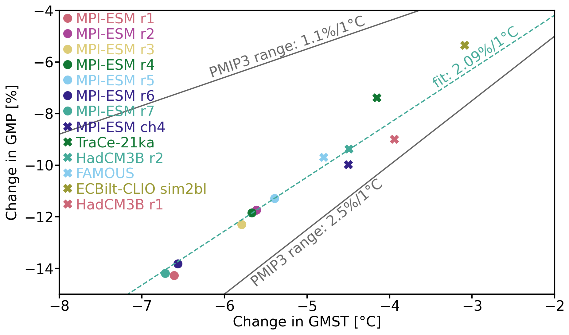
Figure 12 Hydrological sensitivity during the LGM and Holocene: percentage change in LGM-to-Holocene GMP against the change in GMST. The line indicates a 2 % change in precipitation per degree of temperature change. The data are fitted linearly with intercept 0.

Precipitation since the LGM is less studied than temperature, and even fewer proxy reconstructions of hydroclimate exist. There is also no data product like the LGMR, which can be used for comparison of spatial patterns. Therefore, we consider simulated hydrological sensitivity to contextualize our results (Fig. 12). The Clausius–Clapeyron relation estimates a 7 % change in saturation water vapor per degree temperature change. This is further constrained based on the surface energy balance and its effect on evaporation and water availability, such that a realistic range for precipitation change per degree temperature change is 1 %–4 % (Li et al., 2013). Here, we find a hydrological sensitivity of about 2.09 % per degree change in GMST. This agrees with the ranges given for CMIP5/PMIP3 equilibrium simulations by Li et al. (2013) of 1.5 %–3 % per degree Kelvin and Rehfeld et al. (2020) of 1.1 %–2.5 % per degree Kelvin.

5.2 Increasing state dependency of variability with timescale

5.2.1 Increased standard deviation and spectral power of surface temperature during the deglacial transition

For all moments of surface temperature, we find that state dependency generally increases with timescale. Simultaneously, the ensemble simulates a reduction in the spread of temperature distributions towards longer timescales with the overall largest values during the Deglaciation. On annual scales, areas of large standard deviation often exhibit large mean changes, too, but this does not hold for longer timescales. At decadal and centennial scales, standard deviation is largest over the high-latitude oceans, particularly in areas with seasonal sea ice cover and for the Deglaciation in the North Atlantic in response to the changes in the Laurentide ice sheet. Because the sea ice cover shrinks with warming and increases during periods of abrupt cooling, standard deviation is larger for the Deglaciation than for the LGM and Holocene across timescales (Fig. S26). This importance of sea ice for local variability is in line with results from Ellerhoff et al. (2022).

The ratio of LGM-to-Holocene variance mostly shows higher LGM variance, with values between 1 and 2 (Tables 2 and S1). These results resemble those of Rehfeld et al. (2018), who found ratios between 1 and 3 on interannual to decadal scales based on CMIP5/PMIP3 equilibrium simulations. The smaller Holocene Equator-to-pole temperature gradient, itself the result of polar amplification, has been suggested as the reason driving the smaller Holocene variability in comparison to the LGM (Rehfeld et al., 2018). Similarly, Shi et al. (2022) conclude that interannual temperature variance in PMIP3/4 LGM simulations is 20 % higher than in PI simulations as a consequence of an increased meridional temperature gradient, in particular at mid-latitudes. Indeed, we find an enhanced meridional temperature gradient during the LGM for some regions and models, which is correlated with the temperature gradient, including at mid-latitudes. However, in other regions and models, we find no such large-scale increase in the gradient nor a correlation to the variance ratio (Fig. S31).

Few model–data comparisons of variance exist that include the LGM. When comparing the LGM and Holocene, proxy reconstructions show that LGM variance is globally about 4 times higher on timescales from 500 to 1750 years (Rehfeld et al., 2018). The differences we find here are smaller (Table 2). For PMIP3 simulations, Rehfeld et al. (2018) similarly found a smaller simulated than reconstructed ratio. Simulated LGM and Holocene spectra resemble each other in their general shape, with increasing scaling variability towards longer timescales. The absence of a characteristic timescale in a stochastic process leads to such scaling behavior with similar statistical properties across scales (Mandelbrot and van Ness, 1968; Ellerhoff and Rehfeld, 2021). Both global and regional spectra (Figs. 11, S21, S22) suggest inter-model differences in scaling and scale breaks. Investigating these in greater detail by computing scaling factors that quantify the relationship between timescale and variability and identifying scale breaks could shed more light on the nature of the scaling behavior. Scaling has been suggested to differ between glacial and interglacial climates (Huybers and Curry, 2006; Nilsen et al., 2016; Lovejoy, 2015; Rypdal et al., 2013; Roe and Steig, 2004), and we also find state-dependent features (Fig. 11). This is in contrast to the lack of state dependency between global spectra of equilibrium LGM and PI simulations found by Ellerhoff et al. (2022). Since the differences are especially apparent on longer timescales, this might point towards the long-term memory effects or transient forcings missing in such equilibrium simulations.

The Deglaciation shows enhanced levels of variance in comparison to the LGM and Holocene on decadal and centennial timescales (Fig. 5d, g) and larger spectral power above centennial scales (Fig. 11e). Northern high latitudes are the largest source of this state dependency, with further significant state dependency in high southern and northern mid-latitudes (Fig. 5d, g). This reflects the dynamic nature of the Deglaciation with the melting of ice sheets, the resulting freshwater flow, and the subsequent reorganization of the climate system. The enhanced variability in the spectra matches the oscillatory behavior that Clark et al. (2012) described, especially on and for millennial scales.

Comparing simulations and reconstructions, Zhu et al. (2019) argue that simulated and reconstructed temperature variability agree on the global scale. That analysis considers long proxy records and reconstructions reaching back to 5 Myr BP and three of the simulations used in this paper: TraCE-21ka, LOVECLIM DG_ns, and ECBilt-CLIO. With respect to agreement on the global scale, our results agree when comparing the simulations to the LGMR. On local and regional scales, however, climate models have repeatedly been found to underestimate variance on longer timescales (Laepple et al., 2023). Similarly, we find notable differences between regional patterns in the LGMR and the simulations (see Fig. S19).

Considering the longer timescales included in the global spectra, some of the MPI-ESM runs do fall into the range suggested by reconstructions (Fig. 11). The LGMR only falls in the range close to millennial timescales. It shows a steep increase in LGM spectral power towards longer timescales, which translates into an increasing LGM-to-Holocene ratio that is unlike that of most simulations in the ensemble. However, proxy records covering both the LGM and the Holocene are sparse, and both Shi et al. (2022) and Rehfeld et al. (2018) suggest considerable spatial heterogeneity in the variance ratios. The sparse sampling of variance around the globe likely biases the LGMR and thus the comparison. While the LGMR exhibits more similar levels of variability to most of the ensemble, comparison to the other reconstructions suggests a lack of simulated regional variability on multi-decadal timescales and beyond. The difference between the LGMR and other reconstructions leaves uncertainty around the models' abilities to capture climate variability and thus a potential lack of variability in future simulations with consequences for projected changes in the frequency and intensity of extremes. To decrease this uncertainty, our findings can provide a basis for more in-depth model–data comparisons of simulated variability during periods of warming. Realizing the full potential of such an analysis requires an ensemble of coordinated experiments using common protocols (as for some of the simulations here) and improved reconstructions of past variability.

Table 2 Summary of LGM-to-Holocene changes in the moments. For every moment and timescale, the values according to model complexity are listed as ESMs, GCMs, EMICs, and EBM. For the mean, the absolute value of the difference is listed; for the other moments, the ratios are. Ratios are first computed for the individual simulations (see Tables S1 and S2 for surface temperature and precipitation, respectively) and then averaged by category. For EMICs, this only includes ECBilt-CLIO here. Note that, on centennial scales, the ESM and GCM categories include more simulations (MPI-ESM r3 and r4 and FAMOUS) than on the annual and decadal scale, leading among other things to a difference in average mean change. It shows that centennial Holocene skewness of ECBilt-CLIO is very close to zero, which produces a very large EMIC ratio. Very large ratios, as for the skewness of centennial precipitation distributions, are a result of moments very close to zero for the LGM and Holocene.

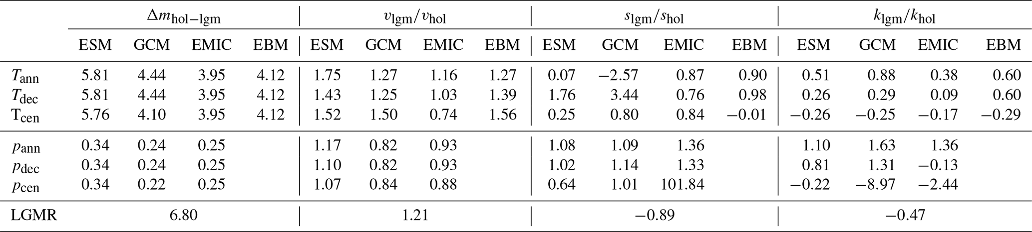
5.2.2 Larger absolute surface temperature skewness and kurtosis towards longer timescales

Temperature skewness and kurtosis, describing the asymmetry and heaviness of the tails of a distribution, respectively, deviate more from zero towards longer timescales, indicating more non-Gaussian distributions and changes in extremes (Figs. 5, S5). During the Deglaciation, mid- and high latitudes show enhanced values of skewness and kurtosis in ESMs and GCMs. Changes in skewness can be an early warning signal of abrupt changes (Skelton et al., 2020; He et al., 2013; Guttal and Jayaprakash, 2008). The simulations in our ensemble undergo large-scale changes that can, at times, be abrupt in response to the prescribed forcings and boundary conditions. Regionally, there may be abrupt change due to internal dynamics of atmosphere, sea ice, ocean, or land surface. As our analysis computes variability over the whole LGM, Deglaciation, and Holocene, it is ill-suited to determine whether skewness changes occur locally or regionally ahead of the abrupt changes. This would instead require an investigation into skewness changes over time. Such an analysis would be of particular interest if it included high-resolution proxy data for key variables experiencing abrupt change and for potential tipping elements.

The LGMR contains some enhanced tropical skew and kurtosis, mainly restricted to the Atlantic and continental areas (Fig. S19). During the Deglaciation, the LGMR shows a pattern of negative skew in the North Atlantic consistent with most simulations with any kind of meltwater forcing. It further exhibits state dependency in the spatial patterns of skewness and kurtosis and an increasing global mean kurtosis from the LGM to the Holocene (Fig. S5i). On the other hand, the LGMR shows very few areas of significant deviations from normality and patterns that are generally more smooth than almost all simulations. Here, we use the LGMR ensemble mean as the basis of all computations. Individual ensemble members consistently show larger standard deviation with common spatial patterns (not shown). For skewness and kurtosis, however, patterns are very inconsistent between ensemble members but, as for the ensemble mean, with mostly Gaussian distributions. This is likely related to the data assimilation, as an ensemble Kalman filter assumes that the state vectors are Gaussian (Evensen et al., 2022). While this assumption works for many weakly non-linear systems (Evensen et al., 2022), it is likely insufficient for the tails of the distribution. Furthermore, the higher-order moments are affected by the spatial averaging inherent in field reconstructions from individual proxy sites (Director and Bornn, 2015; McKinnon et al., 2016; Haylock et al., 2008). Due to the sparse coverage in space and time of the proxy records, they only provide weak constraints during the assimilation, especially further back in time. This likely also explains why the variability in the LGMR is largest during the LGM, when proxy availability is smallest. A comparison at individual proxy locations could shed more light on model–data differences and similarities and could ascertain whether the LGMR indeed has too little variability, as indicated by its differences from both simulations and other proxy reconstructions.

5.2.3 Precipitation distributions show trend towards drier and less extreme years in the tropics from the LGM to the Holocene

For precipitation, mean changes are similarly varied as for surface temperature, with a global mean LGM-to-Holocene wetting of 0.15–0.39 mm d⁻¹. The ESMs and GCMs simulate some drying towards the Holocene over the tropical oceans, with wetting almost everywhere else. The moments are generally largest on annual timescales. In the tropics, ESMs and GCMs show some state dependency but not as much as for temperature. Tropical precipitation mostly decreases from the LGM to the Holocene, especially over the ocean. Over the tropical oceans, standard deviation can similarly decrease from the LGM to the Holocene, while it increases almost everywhere else. During the Deglaciation, some high-precipitation years remain, as indicated by the unchanged positive skewness and kurtosis. For the Holocene, however, annual higher-order moments are generally smaller in comparison to the LGM. Towards longer timescales, standard deviation decreases significantly and shows very little state dependency. For skewness and kurtosis, the tropical peaks diminish, but, instead, areas of larger skew or kurtosis emerge in the mid- and high latitudes, especially during the Deglaciation. So, while annual distributions show that there are extreme-precipitation years in the tropics, decadal and centennial distributions demonstrate that such extreme conditions rarely persist for whole decades or centuries. For skewness, dry regions are generally associated with positive skew, since only a high-value tail can exist for low mean precipitation. This is why precipitation mostly has positive skewness.

Some GCM and ESM runs show bipolar skewness patterns between the hemispheres but disagree on whether the negative skewness is in the Northern Hemisphere (MPI-ESM, HadCM3B) or Southern Hemisphere (TraCE-21ka). These bipolar patterns appear in response to meltwater forcing (see Sect. 5.3). The spectra show little state dependency on annual to multi-decadal timescales (Fig. 11i, j). For centennial timescales and longer, the Deglaciation shows a strong increase in variability, strongest in the tropics (Figs. S23 and S24), setting it apart from the LGM and Holocene. The LGM and Holocene differ to a lesser degree but start diverging on centennial timescales, although the simulations disagree whether the LGM or the Holocene has stronger spectral power.

5.3 Dependence of surface climate variability on external forcings

While ice sheet changes, meltwater fluxes and volcanism all have characteristic timescales, differences in these forcings cause variability changes on other timescales as well. As such, forcings, through their non-linear interactions with faster components of the climate system, impact variability on timescales shorter than their characteristic timescales. Conversely, they also impact slower components and thus variability on longer timescales. This implies that, even when investigating variability on short, e.g., interannual, timescales, the initial state of slower components like the oceans can affect simulated variability.

For ice sheet reconstructions, we compare ICE6G with GLAC1-D, which has a more extensive but lower glacial ice cover. The reconstructions have temporal resolutions of 500 and 100 years, respectively. While the reconstructions were interpolated for MPI-ESM r1–7, this difference in the underlying timescale will still affect centennial variability and likely explains some of the increased variability found for simulations using GLAC1-D in comparison to those using ICE6G (see Fig. 6). For the northern latitudes, the comparison indeed reveals a general association of GLAC1-D with larger standard deviation during the LGM and Deglaciation (Fig. 6). On the other hand, GLAC1-D is associated with reduced standard deviation across timescales in parts of the Southern Ocean during the Deglaciation and Holocene related to less variance in sea ice (Fig. S26). Towards longer timescales, the simulations with GLAC1-D are both more positively and negatively skewed, in particular for the Deglaciation. The chosen ice sheet reconstruction thus significantly impacts variability, especially for temperature, and behavior at the tails of the distributions on annual to millennial timescales. However, there is considerable uncertainty in ice sheet reconstructions and corresponding meltwater releases (Stokes et al., 2015; Abe-Ouchi et al., 2015; Ivanovic et al., 2016), an uncertainty that simulated variability thus retains. Many of the differences between simulations using GLAC1-D and ICE6G can be attributed to their associated meltwater protocols.

A bipolar skewness pattern indicates a meltwater pulse in the area of negative skewness. GLAC1-D introduces meltwater pulses, in particular MWP-1A and MWP-1B, mainly in the Northern Hemisphere. These lead to a freshening of North Atlantic surface water and a slowdown of the Atlantic Meridional Overturning Circulation. As a result, the Northern Hemisphere cools and experiences more cold outliers (negative skewness), while the Southern Hemisphere warms. In ICE6G, on the other hand, MWP-1B is mainly released into the Southern Ocean, counteracting and reducing the dominating bipolar pattern. In TraCE-21ka, the most abrupt freshwater pulse (MWP-1A) is mostly imposed as a freshwater flux into the Southern Ocean and, as such, leads to an opposite pattern in skewness. Kurtosis, similarly, is stronger in GLAC1-D simulations during the LGM and Deglaciation, an effect that grows towards longer timescales. There is a general ranking of simulations by meltwater protocol with variability increasing from no-melt to melt-uniform and finally melt-routed. Since simulations are generally believed to lack variability at least regionally (e.g., Laepple et al., 2023; Weitzel et al., 2024; Rehfeld et al., 2018), this supports the usage of the melt-routed protocol. Since meltwater forcing has such a strong association with variability and the overall deglacial climate evolution (Snoll et al., 2024), variability could help constrain meltwater releases. However, this would require identifying models with high skill regarding simulated variability, currently hindered by large uncertainties in reconstructed variability. Furthermore, tuning meltwater to reproduce reconstructed variability alone is likely too simplified an approach (Weitzel et al., 2024).

Volcanism has the largest impact on annual scales, as it introduces short-term cooling events. However, its impacts are evident on longer timescales as well through non-linear interactions with other components of the climate system, as also noted by, for example, Ellerhoff et al. (2022). This is particularly apparent in the spectra, where volcanism raises the power across and especially on decadal to centennial timescales (Fig. 11). Volcanic forcing mostly increases standard deviation and reduces positive temperature skew across timescales and kurtosis on annual scales as high-temperature outliers become less likely and low-temperature outliers become more likely in response to the negative radiative forcing imposed.

5.4 Dependency of surface climate on model complexity suggests necessary minimal complexity

Our results suggest that there is a required minimal complexity for modeling the variability in surface climate. The EBM only reflects the linear response and does not possess the complexity required to capture changes beyond the mean, while simple models dedicated to variability might (see Lovejoy et al., 2021; Schillinger et al., 2022). The increasing resemblance of the EBM's moments to those of the more complex models towards longer timescales (Fig. S5), on the other hand, suggests that, at the global scale, centennial moments are dominated by the linear response to external forcings. This does not account for spatial patterns, though, which the EBM fails to capture.

The EMIC simulations provide a far better approximation of standard deviation of temperature but fall off for the extreme tails and for precipitation as a whole. The latter suggests that the EMICs lack variability in atmospheric dynamics. The spectral power of the EMICs is almost always on the lower end of the ensemble, further indicating a lack of energy transfer between scales. As such, while they can match variability in proxy reconstructions on the global level (cf. Zhu et al., 2019), they are limited for studies of regional variability. The EMICs included here have reduced atmospheric complexity. This will affect simulated variability and could be different in other EMICs as it is for GCMs.

Among GCMs and ESMs, providing a ranking of simulated variability proves difficult due to the sparse spatial coverage of reconstructions and the lack of literature studying variability during the Deglaciation, although first attempts have been made (Weitzel et al., 2024). Moreover, at the level of complexity of GCMs and ESMs, chosen forcings cause differences between simulations at least as much as the chosen model and its complexity. Due to substantial differences in forcings and boundary conditions inherently arising from different research foci, it can be hard to identify the sources of differences between simulations from different models of similar complexity. While there are some common patterns that emerge, the simulations also disagree in many areas with respect to magnitude and even direction of changes. This variety in the ensemble can be hidden when considering multi-model means. An experimental design geared towards understanding the roles of feedbacks on surface climate variability must take into account external forcing and boundary condition changes, distinguishing interactive effects and prescribed changes in boundary conditions which may, or may not, be physically consistent with the climate evolution. Given the impact of meltwater forcing and its uncertainties, simulations with interactive ice sheets are of particular interest to the study of climate extremes in response to mean changes.

6 Conclusions

The variability in surface climate has undergone considerable changes since the LGM, along with an increase in GMST. Here, we investigate changes in several indicators of variability from the LGM to the Holocene. These include standard deviation and power spectra but also the higher-order moments of skewness and kurtosis, which have, to our knowledge, previously been used only in studies of present-day and future climate. The warming ranges from 3.0–6.6 °C in the ensemble of 15 transient simulations from models of varying complexity presented here. This result agrees with the estimates found in reconstructions, which also cover a large range. On the whole, we can confirm our hypotheses as (1) the variability between LGM and Holocene changes with the mean background state for both surface temperature and precipitation, and the variability during the Deglaciation is generally larger in comparison. Furthermore, we find that (2) state dependency increases from annual to millennial scales and that the forcings impact variability on all, not just their characteristic timescales, and that (3) there is a minimal complexity needed to simulate adequate levels of variability. In particular, we find that the variability of surface temperature and precipitation depend on the following:

1. Background state. Overall, state dependency of variability increases towards longer timescales. Standard deviation of surface temperature is larger during the LGM than the Holocene, whereas it is the opposite for precipitation. The LGM has little overall temperature skewness and kurtosis, whereas there can be areas of large skewness and kurtosis during the Holocene. For precipitation during the LGM and Holocene, state dependency can be found to some degree on all timescales and for all moments, but no clear patterns emerge. Beginning on decadal scales, the Deglaciation, as the transition between a cold and warmer interglacial climate state, stands out as a period of enhanced variability in comparison to the LGM and Holocene. This is marked by increased variance, more skew (both positive and negative), and larger kurtosis in most simulations.

2. Timescale. Towards longer timescales, the distributions of temperature show a decrease in variance, more absolute skew, and an increase in kurtosis, i.e., enhanced non-Gaussianity. For precipitation, variance decreases, too, while changes to the higher-order moments are mainly limited to the Deglaciation and differ by simulation and region. Volcanism, meltwater forcing, and ice sheet changes affect the distributions of surface temperature and precipitation the most on their characteristic timescales, but their effects can be detected from annual to millennial timescales.

3. Model complexity. Both the EBM and EMICs fail to reproduce patterns of variability found in the (sparse) reconstructions and do not resemble those in the more complex models. In our ensemble, the complexity of a coupled ocean–atmosphere GCM is at least necessary to produce realistic variability patterns. For the GCM and ESM simulations, on the other hand, differences in forcing protocols and boundary conditions play a larger role than model complexity in determining variability in surface temperature and precipitation.

To reach levels of variability comparable to reconstructions, simulations depend upon adequate levels of externally forced variability, including from volcanic forcing, and internal variability. The contribution of internal variability requires at least the minimum complexity of the GCMs in this study. Nevertheless, comparison to some reconstructions of past climate suggests that simulations might lack variability, especially regionally and from multi-decadal timescales onward. While the LGMR provided a first point of comparison, the comparison also raises questions about a potential loss of variability in field reconstruction methods when contrasted to other reconstructions. However, further conclusions necessitate an in-depth model–data comparison, which is limited by the small number of available proxy records, especially for precipitation. Since an improved understanding of the variability in surface climate is crucial, for example, because of its relation to extremes and freshwater availability, a comparison to 20th-century observations could provide clearer evidence on the models' abilities, at least for short timescales. This could complement model evaluation efforts like CMIP and PMIP.

Several factors have emerged that could advance the evaluation of simulated variability and allow a ranking of models: improved benchmarks from reconstructions, more simulations with consistent protocols, ensemble of varying initial conditions, and high-resolution snapshot simulations of past climates. The latter would allow an analysis of the changes in frequencies of extremes against regional mean changes and how extremes on short timescales transfer to longer timescales. As such, it could elucidate the role of higher-order moments in the evaluation of model simulations going forward.

Our results demonstrate that the Deglaciation stands out in comparison to the LGM and Holocene as a period of warming. However, an open question remains to what degree our results hold for future warming. To resolve this question, it is necessary to understand how much the increased variability is related to overall warming versus the initial state with large Northern Hemisphere ice sheets. Interactions between dynamics, forcings, and mean state lead to complex changes in the distributions of surface climate variables. This implies potential changes to extremes on timescales from years to centuries, requiring further investigation.