the Creative Commons Attribution 4.0 License.
the Creative Commons Attribution 4.0 License.
 | 04 Feb 2025
New probabilistic methods for quantitative climate reconstructions applied to palynological data from Lake Kinneret
Timon Netzel
Andrea Miebach
Thomas Litt
Andreas Hense
Quantitative local paleoclimate reconstructions are an important tool for gaining insights into the climate history of the Earth. The complex age–sediment–depth and proxy–climate relationships must be described in an appropriate way. Bayesian hierarchical models are a promising method for describing such structures.
In this study, we present a new age–depth transformation in a Bayesian formulation by determining the uncertainty information of depths in lake sediments at a given age. This enables data-driven smoothing of past periods, which allows better interpretation.
We introduce a systematic, machine-learning-based way to establish probabilistic transfer functions which connect spatial distributions of temperature and precipitation to the spatial presence of specific biomes. This includes consideration of various machine learning (ML) algorithms for solving the classification problem of biome presence and absence, taking into account uncertainties in the proxy–climate relationship. For the models and biome distributions used, a simple feedforward neural network provides the optimal choice of the classification problem.
Based on this, we formulate a new Bayesian hierarchical model that generates local paleoclimate reconstructions. This is applied to plant-based proxy data from the lake sediment of Lake Kinneret (LK). Here, a priori information on the recent climate in this region and data on arboreal pollen from this lake are used as boundary conditions. To solve this model, we use Markov chain Monte Carlo (MCMC) sampling methods. During the inference process, our new method generates taxa weights and biome climate ranges. The former shows that less weight needs to be given to Olea europaea to ensure the influence of the other taxa. In contrast, the highest weights are found in Quercus calliprinos and Amaranthaceae, resulting in appropriate flexibility under the given boundary conditions. In terms of climate ranges, the posterior probability of the Mediterranean biome reveals the greatest change, with an average boreal winter (December–February) temperature of 10∘C and an annual precipitation of 700 mm for Lake Kinneret during the Holocene. The paleoclimate reconstruction for this period shows comparatively low precipitation of about 400 mm during 9–7 and 4–2 cal ka BP. The respective temperatures fluctuate much less and stay around 10 °C.
- Article
(9167 KB) - Full-text XML
- BibTeX
- EndNote


Local paleoclimate reconstructions reveal information on the climatic history of relatively small regions. In the last few decades, a lot of reconstructions were published, which showed the advantages and disadvantages of the respective methodologies. One promising way is the idea of the indicator species approach, which is the basic of the model used in this study. Here, plant distribution maps are linked to recent climate data to define a climate range where the corresponding taxon occurs. Finally, when considering multiple taxa, these climatic ranges can be combined to determine the mutual climatic range (MCR).
We follow the idea of Kühl et al. (2002), who developed a probabilistic interpretation of MCR. This addresses the problem of overfitting by calculating uncertainty ranges for each taxon. These were initially based on two- or three-dimensional Gaussian probability density functions (PDFs), which is why this is called the PDF method. This basic concept was extended and applied for both local and spatial climate reconstructions. For example, Kühl and Litt (2003) calculated January and July temperatures for three sites in central Europe during the Last Interglacial. Subsequently, spatial reconstructions of Europe were performed in Gebhardt et al. (2008) for the Eemian, in Simonis et al. (2012) for the Late Glacial and Holocene, and in Weitzel et al. (2019) for the mid-Holocene (MH). Over time, more complex machine learning (ML) methods, such as the generalized linear model and quadratic discriminant analysis (QDA), are used to determine the transfer functions (e.g. Litt et al., 2012; Weitzel et al., 2019). Schölzel (2006) describes the PDF method in the context of a Bayesian hierarchical model (BHM) and calls it the Bayesian Indicator Taxa Model (BITM). This has the advantage that additional prior information can regulate the transfer functions and thus the entire climate reconstruction. Among others, the BITM was applied in Neumann et al. (2007) for Birkat Ram in Israel and in Thoma (2017) for Lake Prespa in Greece.
The basis of the climate reconstruction used in this work is first presented by Schölzel (2006). This is another BHM, the so-called Bayesian biome model (BBM). In this process, certain plant taxa are assigned to different biomes. These are groups of taxa that have similar vegetation zones under comparable climatic conditions (Prentice et al., 1992). One advantage of the BBM is that no recent distribution maps for every plant occurring in the core, but only for the biomes used, is needed. Applications of this model can be found in Schölzel (2006), Litt et al. (2012), and Stolzenberger (2017) for the Dead Sea. A first application of climate reconstructions to data from Lake Kinneret (LK) is shown by Thoma (2017), who used the time series information of the two major biomes which can be deduced from the LK core. The resulting BBM-based paleoclimate reconstruction did show too little variability in temperature and precipitation, suggesting that at least a three-biome-model approach (Mediterranean, Irano-Turanian, Saharo-Arabian) as a basis for the BBM should be used. For numerical reasons, a virtual or undefined biome will be introduced. The BBM also allows reconstructions based on prior climate data. These come, for example, from other studies that suggest possible climate ranges for the reconstruction site and period (Schölzel, 2006). Once set, they cannot be adjusted during the reconstruction process.
Although the abovementioned methods for reconstructing the local climate are already quite well elaborated, they still need more modifications and improvements, which can be summarized in four points:
-
Quantitative inclusion of age uncertainty;
-
Enhancing the Bayesian biome model (BBM) by
- a.
evaluating effects of potential human impacts upon the climate reconstruction,
- b.
treating in a flexible way the spatial taxa or biome vs. climate relationships (transfer functions),
- c.
including on the prior level user-defined (potentially subjective) decisions with respect to taxa selection, transfer function parameter values, and a choice of model structure.
- a.
The need for the last point is due to the assumption that relationships between recent climate and plant distribution have not changed during the reconstruction period. A central message of our approach is that the whole chain of modifications according to points 1 and 2a–c is based on Bayesian statistical methods together with its numerical implementation. This provides a clear advantage over past attempts, which have mostly seen single layers of the methods described below. As one of the reviewers commented, this will “automate some ad hoc decisions in the interests of reproducibility and ease of use and raise the quality of reconstructions”.
This traceability of the proposed method for calculating quantitative paleoclimate reconstructions results from the increased automation and the Bayesian statistical modeling rather than from additional assumptions. The Bayesian approach not only reconstructs a climate variable like temperature or precipitation but also attempts to model the full joint probability density of the climate variables given the proxy data at a given age. This stochastic view includes the most probable climate and its related uncertainty. By this, it will provide additional insights into the importance of the proxies studied and thus extend the knowledge from previous studies. As a worked-out example, we will apply the new model to botanical proxy data (pollen) from LK. A comparison is possible following the results from previous reconstruction studies of paleoclimate information in the vicinity of LK (Schiebel and Litt, 2018; Miebach et al., 2022; Orland et al., 2009), specifically the Dead Sea region (Litt et al., 2012). The latter exhibits certain deficits like biases at recent time slices or extensive variability during Holocene times. The further aim of the present study is to evaluate the potential of those abovementioned additional environmental data in the vicinity of LK to enhance similarities and reduce differences between quantitative climate reconstructions at LK based on the previous BBM methods and the information content of the additional qualitative data.
The general approach for inclusion is a Bayesian-statistics-based data assimilation of the new environmental data (via a likelihood) into the previous reconstruction forming the prior. The resulting posterior will not only provide the most probable reconstruction of the paleoclimate state given both types of input data but also an uncertainty estimate. This allows a comparison of the prior reconstruction with the posterior one and an assessment of the gain of information by the assimilation without the need for independent data. The theoretical concept presented in this study readily extends to the inclusion of such independent data, which is a task for future work. In addition, data already available on lake-level fluctuations can be used as independent proxies, at least for precipitation changes, for comparison with pollen-based reconstructions (Lake Kinneret: Hazan et al., 2005; Vossel et al., 2018. For regional scale changes at the Dead Sea: Litt et al., 2012; Stein et al., 2010).
These motivations lead to the following structure of the presented work. In Sect. 2 we give an overview of the study area. Section 3 first deals with observed palynological data serving as input, then the quantitative inclusion of the age–depth relation and its uncertainty is described (bullet point 1), followed by the actual probabilistic reconstruction model treating bullet points 2 and 3, followed by an introduction of the flexibility in the probabilistic transfer functions. The resulting individual modules of the proposed Bayesian framework are described in detail. Section 4 presents the results of our new reconstruction method using the LK palynological data sets. These are then discussed, summarized, and compared to previously available reconstruction, with possible extensions suggested in Sects. 5 and 6.
The study area and the details of its plant geographical territories are show in Fig. 1b with the mean annual precipitation sum at a high resolution from a subjective analysis (Zohary, 1962) in Fig. 1a. LK has a maximum water depth of ca. 42 m and a surface area of ca. 169 km2 (21×12 km at the maximum). The catchment area comprises 2730 km2 (Berman et al., 2014).
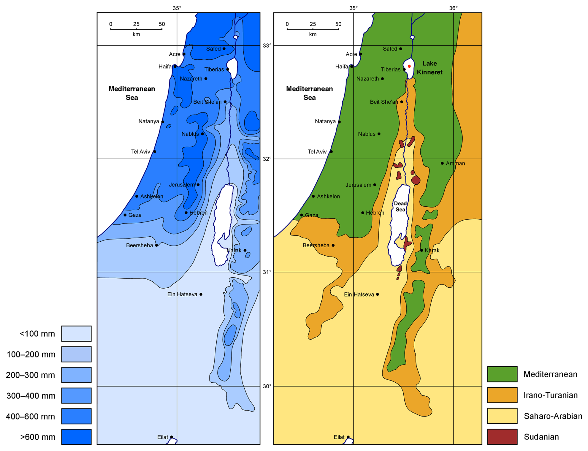
Figure 1Mean annual precipitation and plant geographical territories of the southern Levant (after Miebach et al., 2019, based on Zohary, 1962). The Kinneret is situated in the north close to Tiberias, and the Dead Sea is visible in the middle part of the figures.
The Sea of Galilee occupies the LK basin along the active Dead Sea fault. It is developed by several tectonic processes (Ben-Avraham et al., 2014). Soils such as terra rossa and rendzina form the surface cover of the Galilee Mountains (Dan et al., 1972). Alluvial and lacustrine sediments of Pleistocene to Holocene ages fill the Jordan Valley north and south of the Sea of Galilee (Sneh et al., 1998).
Switching to the climate data on the grid of 0.5°×0.5° defining the Climate Research Unit (CRU) data set (Harris et al., 2020) in Fig. 2a and b shows the spatial distribution of the mean December to February temperature (TDJF) and annual precipitation (PANN) that we will examine in more detail in this study. In particular, this means that this combination will be reconstructed for the LK. The Mediterranean climate with hot, dry summers and mild, wet boreal winters is typical of northern Israel, as shown by the Koeppen–Geiger classification Csa in the climate diagram of LK in Fig. 2c. The basin of the lake is characterized by 400 mm mean annual precipitation and 21 °C mean annual temperature. The surrounding mountains, however, experience PANN rates of up to >900 mm and annual temperatures of less than 15 °C. The climate diagram reflects these relatively large variations, which result from the 0.5°×0.5° horizontal resolution of the CRU data set. Altogether, 90 % of the precipitation in the north of Israel comes from so-called Cyprus lows that form over the eastern Mediterranean. These mainly occur from October to May, with the heaviest rainfall between December and March (Ziv et al., 2014).

Figure 2The mean December–February temperature TDJF (a) and annual precipitation PANN (b) based on the current version (4.07) of CRU data and the period 1961–1990. The black dot marks the location of LK. A climate diagram of the grid point closest to LK is shown in panel (c), based on these CRU data. Panel (d) depicts the coarse-grained biome definitions used in this work.
Furthermore, Fig. 2d shows the biome distributions considered in this work. The colored areas distinguish the following biomes: the Mediterranean, the Irano-Turanian, the Saharo-Arabian, and the unspecified biome which is needed for numerical reasons in the classification models (see below).
We can see that the majority of the lake’s watershed can be ascribed to the Mediterranean biome, while the southern lakeshore borders the Irano-Turanian biome (Zohary, 1962). The Mediterranean biome is distributed in areas exceeding 300 mm of PANN (see Fig. 2b). The climax vegetation is dominated by trees and shrubs. Typical plants are Quercus ithaburensis, Q. boissieri, Q. calliprinos, Olea europaea, Pistacia lentiscus, Arbutus andrachne, Ceratonia siliqua, Pinus halepensis, and Sarcopoterium spinosum (Danin, 1988; Zohary, 1982). The Irano-Turanian steppe grows in areas below 300 mm of PANN (see Fig. 2b). The biome is rich in semi-shrubs, annual herbs, and geophytes. Common taxa are Artemisia herba-alba, Thymelaea hirsuta, and various Poaceae and Amaranthaceae (including Chenopodiaceae) (Danin, 1992; Zohary, 1982) The Saharo-Arabian desert vegetation type occurs in the southern part, where the mean annual precipitation falls below 100 mm. It is a vegetation type with sparse plant cover and low diversity. Important representatives of the Saharo-Arabian vegetation are Zygophyllum dumosum, Retama raetam, Tamarix nilotica, Atriplex halimus, and other Amaranthaceae. Sudanian vegetation occupies tropical oases of the Jordan Valley. Mainly trees and shrubs such as Maerua crassifolia, Acacia raddiana/Acacia tortilis, Balanites aegyptiaca, and Ziziphus spina-christi compose this vegetation type (Zohary, 1962). This oasis vegetation is included in the Saharo-Arabian biome.
3.1 Material
The material used in this study originates from lacustrine sediment cores from the central Sea of Galilee. It was recovered in March 2010 during a drilling campaign within the Collaborative Research Center 806 “Our Way to Europe” funded by the German Research Foundation (DFG). Two parallel cores (Ki10 I with 13.3 m core recovery and Ki10 II with 17.8 m core recovery) were obtained at a water depth of 38.8 m. Both cores were combined to a 17.8 m composite profile. Besides a 25 cm varved sequence at the top, the sediment comprises homogeneous grayish–brownish silts and clays (Schiebel and Litt, 2018).
3.2 Palynology
Additional samples were added to the palynological data sets by Schiebel and Litt (2018) and Langgut et al. (2013) to increase the temporal resolution. The resulting data set consists of 160 samples with a mean resolution of 11 cm. We followed a standard preparation technique by Faegri and Iversen (1989) to extract pollen from the lake sediment (see Schiebel and Litt, 2018, for more details). At least 500 terrestrial pollen grains were identified under a light microscope at 400× magnification with the help of the pollen reference collection from the paleobotanical laboratory at the University of Bonn and pollen atlases (Reille, 1995, 1998, 1999; Beug, 2004). Pollen percentages are based on the terrestrial pollen sum excluding indeterminable pollen grains and obligate aquatic plants to exclude local taxa growing in the lake (Moore et al., 1991). Pollen zonation was adapted from Schiebel and Litt (2018).
3.3 Quantitative inclusion of age uncertainty
3.3.1 Age–depth model
We start with the Bayesian-statistics-based age–depth model from Miebach et al. (2022) to describe the relationship between age and depth. It provides a probabilistic model of the sediment accumulation rate of the core necessary to reach the 14C ages at the available depths within the dating uncertainties. We use the Bacon model implemented in R (R Core Team, 2018; Blaauw et al., 2020). The well-known OxCal dating approach (Ramsey, 2009) is similar to the strategy in the Bacon model, which is explained in detail and compared to OxCal in Blaauw and Christen (2011) and is only briefly described in the following.
Bacon uses a self-adjusting Markov chain Monte Carlo (MCMC) simulation to calculate the conditional probability distribution , where ϕ contains the model parameters, r contains the accumulation rate, m contains the memory effect inherent in the sedimentation, and x contains the measurements such as 14C data. As a result, Bacon describes the posterior (conditional) probabilities of ϕ, r, and m given the age data 14C at the given sediment depth D. However, as we will see in the next section, we are actually interested in the conditional probability of depth D at a fixed age A, which can be derived using the accumulation rates r and applying Bayes' theorem.
3.3.2 Age–depth transformation
Now we will consider how to use the probabilistic information from models like Bacon to calculate a transformation from depth to age. For this purpose, it is useful to look at Table 1, which describes the variables used in this work. Using Bayesian hierarchical modeling techniques, we can determine the joint probability density function (or probability mass function in the case of discrete random variables) of the target variables Y, the age A, the proxy data P, and the required additional parameters Θ. These are, of course, all dependent on depth, but D is only an auxiliary variable due to the coring procedure. Therefore, the full joint probability density/mass function that includes D can be marginalized (integrated) with respect to D. In a second step, we apply the relationship between full, joined, and the necessary conditional and marginal probability distributions. This establishes the following equation:

Y contains the variables we are interested in, e.g., C. Now suppose that D is conditionally independent of P and Θ and thus fully dependent on A. This is exactly the information we obtain from the age–depth relationship. Furthermore, the variables Y should not depend on age if D is given. This assumption follows from the fact that, initially, any information drawn from the sediment core is with respect to depth. Using this, we can transform Eq. (1) as follows:
As we can see, we need a tool for the calculation of the conditional probability distribution of sediment depth D given the age A: ℙ(D|A). This was developed for this work and can be found as a contribution to the rbacon package under the function Bacon.d.Age. Bacon calculates the slopes (accumulation rates) of a series of flexible linear age–depth functions. Their flexibility results from different r in a priori defined regular sections along the depth axis. If a certain age A=a is specified, Bacon.d.Age searches for those sections where intersections between a and the respective age–depth functions exist. In this way, we can calculate probability distributions of depths for each age within the reconstruction period.
ℙ(D|A) obtained in this way indicates which depth has a higher or lower (possibly approaching zero) probability of contributing to Y at a given age. Equation (2) shows that the desired age-dependent target variables Y are calculated by a moving-window (convolution) stretching/compressing operation on the depth axis together with a smoothing of this axis at each sediment depth. The moving windows are derived solely from the age–depth model data and do not necessarily follow a top-hat filter or any other smoothing function.
Figure 3 illustrates the entire process using the arboreal pollen (AP) percentage from LK as an example. The full model results will be discussed below. In this case, the target variable Y is the AP percentage and is shown in Fig. 3a as a function of measured sediment depth. Using the depth–age relation of the most probable age at a given depth, the mean age difference between the studied core intervals of 11 cm thickness is 51 years. Thus, in a first step, we define a regular temporal grid of 50 years resulting in a total of 181 age steps between 0 and 9 kyr BP. Based on the results of the full probabilistic analysis of the sedimentation–time relationship available from the rbacon package, the newly added function Bacon.d.Age determines those depth samples which belong to a given age on the temporal grid with a probability between zero and 1, including the changing sedimentation rates in the lake over the past 9 kyr modeled internally in rbacon. Applying Eq. (2) then weights depths either with near zero or with a finite probability value given an age on the 50-year time grid between 0 and 9 kyr BP in 181 time steps. With this procedure, the approach addresses the full age–depth uncertainty. Since age is a given variable (no longer a random variable, as it is in the conditional probability of age given the sediment depth), in principle, any time-stepping (10, 25, 100 years) could have been chosen, but the 50-year time step is determined by the data set itself.
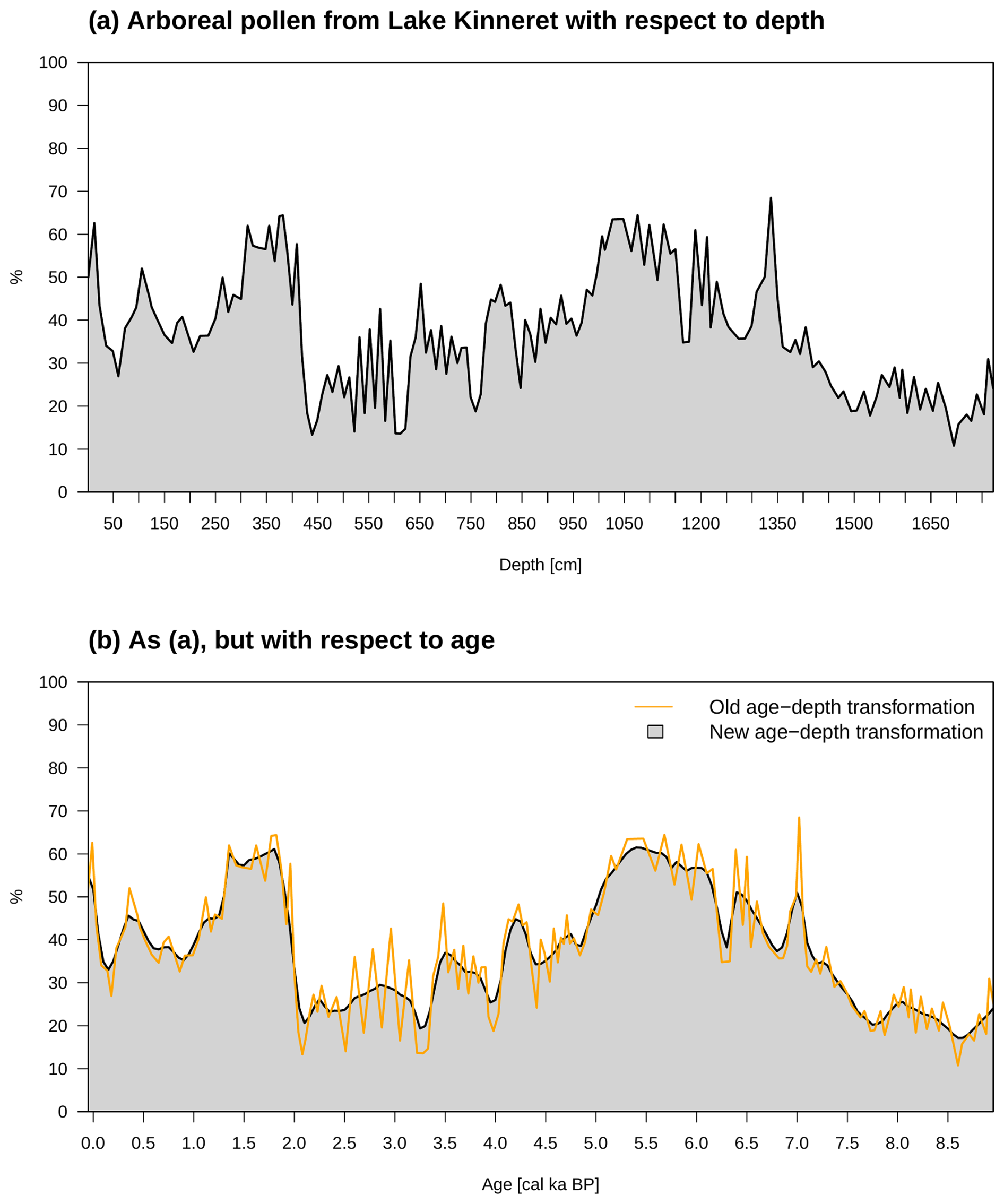
Figure 3The gray areas show the percentages of aggregated arboreal pollen from LK. Panel (a) depicts these data in terms of depth, and panel (b) depicts them in terms of age. On the one hand, in panel (b), we see the result when all probability information ℙ(D∣A) is taken into account (gray area). The orange line, on the other hand, represents the output using the mean values of A.
Using the arboreal pollen percentages from Fig. 3a in Eq. (2), we obtain the result of the new age–depth transformation AP values depicted in Fig. 3b. In contrast, the orange line shows the result when the plant data in terms of depth are linked to the mean age data from the age–depth model.
The standard use of the age–depth relationship, e.g., in Litt et al. (2012), Schiebel and Litt (2018), Torfstein et al. (2015), Neumann et al. (2007), Miebach et al. (2019), and Seppä et al. (2005), is incorporated in Eq. (2), making the Bayesian statistics approach more general as the standard method of age–depth calculation. It is illustrated by the orange line in Fig. 3. It is achieved for a given age by selecting a single sediment depth with a probability of 1, e.g., the depth at which the conditional probability of depths given the age is at a maximum, and then formally computing the integral. No information about the age–depth-related uncertainty is used: only one sediment depth is determined for a given age, clearly a case to be identified as “overfitting”, indicated by the strongly fluctuating behavior of the orange AP percentage curve, which makes interpretations difficult. As a result, this new technique circumvents such problems.
3.4 Enhancing the reconstruction model
In this study, an enhanced and extended version of the BBM/BHM is presented to calculate the quantitative climate reconstruction. The detailed derivation of it can be found in Appendix A, with the final result written as
This is the basic model calculated Nsample times with for different ωi and Ci by systematically sampling from the pools of plant information and transfer function distributions using MCMC techniques. In order to be able to describe this in more detail, certain framework conditions need to be introduced. To this end, we will introduce reference curves based, for example, on AP percentage data from lake sediments (see Fig. 3b). If a reconstruction according to Eq. (3) is performed for certain ωi and Ci, the resulting can be compared with these reference curves. As a similarity measure, the explained variances R2 in the regression of the reference curve vs. the mean or median curve derived from Eq. (3) are used and stored in a variable we call proxy pool PP. Then, the extended BHM can be constructed (the weighting term is omitted for clarity):
At this point, one could add a variety of additional reference curves based on, for example, isotope time series from lake or marine sediments, ice cores, insolation time series, or greenhouse gas information (Netzel, 2023a). However, only proxies derived from botanical information are considered in this work.
We know that some sections of the AP percentage curves have fluctuations that are not due to climate variability (e.g. Panagiotopoulos et al., 2013; Miebach et al., 2016; Neumann et al., 2007; Litt et al., 2012; Schiebel and Litt, 2018). In particular, the anthropogenic influence upon vegetation in the study area (Fig. 2) during the mid- to late Holocene complicates the interpretation of these curves. To account for similarities and to reduce differences between the reference and the reconstruction, the regression between the reference curve and the reconstruction is interpreted as a simple Bayesian data assimilation step, with the reference forming the prior and the reconstruction curve forming the likelihood, explaining an anticipated amount of variance R2. To be in line with the general Bayesian approach, that amount is not a fixed number but is described by a mean value and an uncertainty summarized by the beta distribution with the two shape parameters α1,2:
A sensitivity analysis is performed by varying the mean value of R2 from 25 % to 50 % and 75 % with a typical standard deviation (uncertainty) of 20 %, obeying the constraint that the explained variance can only vary between 0 % and 100 %. On the one hand, this gives the model the ability to capture a sufficiently large range of R2 (Netzel, 2023a), while, on the other hand, additional moderators like human influence are allowed if represented in either the climate reconstruction or the reference data set. The necessary combinations of mean and standard deviation vs. the two shape parameters are given in Table 2.
Table 2Means and standard deviations of beta distributions with the shape parameters α1,2.

This part of the model is the first term on the right of Eq. (4), which we call the proxy pool module.
The second term of Eq. (4) can be analyzed as follows:
gives the model the ability to constrain the reconstructions based on additional climate information from the past. These can be of different origins, for example, other local reconstructions, paleoclimate simulations, or even subjective expert knowledge based on vegetation or other ecological studies. The latter is a common approach in classical Bayesian statistical analysis (Berger, 2013). In the simplest case, it would be a subjective probabilistic statement with a number between zero and 1 (but excluding both) about the climate state Cp given the age and the proxy data. Inclusion of such past climate data information is shifted to future work, e.g., when high-resolution regional paleoclimate simulations become available. The second term on the right of Eq. (6) allows us to insert constraints on the reconstructed modern climate. We define the transition from modern times to the past at 0 cal yr BP (calibrated years before the present), i.e., 1950 CE. This is because the temporal resolution of 50 years limits us, as we can only define the years 2000 or 1950 CE as the most recent period. For such a modern climate, we use the CRU data presented in Fig. 2 and create probability distributions as anchors for the reconstructions. These independent proposal distributions are described by a normal distribution as an approximation for TDJF and a gamma distribution for PANN. All in all, we refer to the above as the prior climate module, which can be summarized as follows (with Unif being the uniform probability density):
This means that reconstructions can be carried out with fewer restrictions even without prior climate information. This is made possible by the use of uniform distributions that encompass the reconstruction period and thus all time slices Nage.
Finally, we consider the third term on the right of Eq. (4) in detail:
Firstly, we assume that the parameters ω and ψ are a priori independent of each other. Then, we state that P is independent of ψ if no C is given. Finally, the updated taxa weights ℙ(P∣ω) are determined under the assumption that they are conditionally independent of A. This means that the additional data used to update the weights are assimilated over the entire reconstruction period. At this point, it is possible to introduce additional prior information for time-continuous reconstructions, e.g., across a full glacial–interglacial cycle. The updating of the taxa weights could be split according to that temporal information such that after assimilation they differ for selected time periods. This approach is not explored further in this study and could be included in future work.
The last term of Eq. (4) is the joint distribution of A and Θ. We assume that all parameters Θ are a priori independent of A. Thus, this distribution can be formulated as follows:
The second term contains the parameters of the transfer functions, and A is assumed to be uniformly distributed if no depth information is available. We see that already in the local reconstruction module in Eq. (3), where the relations between A and D are inserted into our reconstruction scheme. With all the reformulations and simplifications listed above, Eq. (4) can be summarized as follows:
Overall, taxa percentages and climate regions that better fit the constraints of the prior climate and proxy pool modules should be weighted higher. How this is done in detail is described in the following.
In the context of MCMC sampling, we update ℙ(P∣ω) using the random walk Metropolis–Hastings (rwMH) technique, since a corresponding full conditional ℙ(ω∣P) does not follow a probability distribution from which we can sample directly. Without further prior information, we assume a uniform distribution across all taxa K at the beginning of the MCMC simulation:
The respective weights are determined with the help of an additional prior distribution:
Such a Dirichlet distribution allows us to determine the taxa weights as requested above. This means that the taxa weights have values between zero and 1 and add up to 1. The Jeffreys prior hyperparameters () of this distribution give each taxon equal prior weight. Furthermore, these values provide a weaker constraint for determining the posterior taxa weights. This property follows directly from the characteristics of the Jeffreys prior (Gelman et al., 2013).
As described above, we want to sample not only taxa weights but also climate values in the climate feature space of the biome transfer function. In this way, we can identify preferred climate ranges based on the plant data and boundary conditions. The parameters ψ remain unchanged because we assume that they are a good approximation for the Holocene. Instead, we sample directly from the climate space and use ℙ(C∣ψ) from Eq. (3). Again, rwMH is used because we cannot sample directly from the full conditional. In this case, we use double-truncated normal distributions 𝒩t restricted to the climate range of the transfer function as proposal distributions to exclude biologically unrealistic climate values:
The transfer function parameters ψ determine not only the truncation ranges a and b but also the expectation values μ and standard deviations σ.
Figure 4 summarizes graphically how this local reconstruction framework works. The boxes in the upper row contain the input variables, while those in the white boxes are not inferred during the MCMC simulation. The parameters of the transfer functions are defined in Sect. 3.5, and the age–depth relationship is described in Miebach et al. (2022). The upper gray boxes describe the inference of the taxa weights and the climate values via rwMH sampling. This is done by comparing the sampled climate reconstructions (reconstruction module) with additional recent climate data and an AP percentage reference curve (prior climate and proxy pool modules) and constraining them accordingly. These comparisons are made using the independent Metropolis–Hastings sampling. All in all, the procedure presented here leads to the comprehensive extensions outlined above.

Figure 4Directed acyclic graph of the Bayesian framework in Eq. (11). The gray boxes represent the quantities that will be inferred during MCMC sampling, and the white boxes contain fixed quantities. The corresponding arrows represent the mutual dependencies, with their direction pointing to the ascending hierarchical levels, and the additional boxes indicate the respective sampling procedures of the modules contained therein.
3.5 Transfer functions
One objective of this work is to systematically test a variety of possible methods to determine the transfer function from Eq. (3) and select the most appropriate algorithm for the task at hand. For this purpose, we use the R package caret (Kuhn et al., 2019). This stands for classification and regression techniques and provides a variety of models that can be used to solve corresponding problems. The package supplies a simple way to compare the selected models via cross-validation. In this process, the provided data (see Fig. 2) are split into a training and a validation data set. Cross-validation is performed on the training set (James et al., 2013), which accounts for 70 % of all data. Statistical verification distributions result from this, which are used to derive the performance of the models. Cross-validation is also performed for a certain number of different parameters for the respective machine learning (ML) algorithms (model tuning). The entire process is very easily accessible in caret and runs completely automatically after the initial parameters have been defined. The remaining 30 % (hold-out set) is used to validate the models obtained by cross-validation on the remaining 70 %. This has the advantage that they can be tested on an independent data set, further minimizing the risk of overfitting.
As can be seen in Fig. 2d, the defined biomes (minority classes) and the unspecified biome (majority class) are unbalanced. This means that the number of grid points covering the different classes varies largely. In a balanced data set, they would be roughly equal. One could reduce the size of the entire map section so that the groups are more balanced. However, the models then deliver significantly worse and sometimes even unrealistic results. This means a model could provide higher probabilities of occurrence, on the one hand, where the biomes do not occur in the feature space and, on the other hand, where the climate values are biologically unrealistic. This problem is discussed, for example, in Thoma (2017) and in Weitzel et al. (2019). When the map section is enlarged, this problem recedes, especially if the absence values can serve as a boundary. This is the case when the occurrence domain is enclosed by the absence domain in the two-dimensional feature space spanned by TDJF and PANN. The reduction of the map section is analogous to the techniques of random undersampling (Hoens and Chawla, 2013). The majority class is randomly reduced to the size of the minority class, potentially losing important information. In contrast, random oversampling of the minority class risks overfitting. To solve this problem, the Synthetic Minority Oversampling Technique (SMOTE) is used (Bowyer et al., 2011). Here, a minority-class instance is first randomly selected, and its k-nearest minority-class neighbors are determined. A line segment is then formed between one randomly selected neighbor in feature space. A synthetic instance of the minority class is created by selecting a random point along this line (Hoens and Chawla, 2013). SMOTE can only do this with one minority class at a time. Therefore, we use this technique separately for each of the three minority classes compared to the majority class. Finally, all four classes consist of a similar number of data points. These are the input for the calculation of the transfer function in the ML competition, so only the training data are processed with SMOTE. For the model verification on the hold-out set, the original data are used.
Table 3 lists four ML models that we compete against each other. We have removed support vector machines (SVMs) from this list as they are not competitive due to their disproportionately long prediction time. Similar difficulties with SVMs are also found in Jergensen et al. (2020), where an ML competition for forecast models of convective storms is presented.
Venables and Ripley (2002)Venables and Ripley (2002)Leisch et al. (2017)Greenwell et al. (2019)Table 3Machine learning algorithms which are used for the competition.
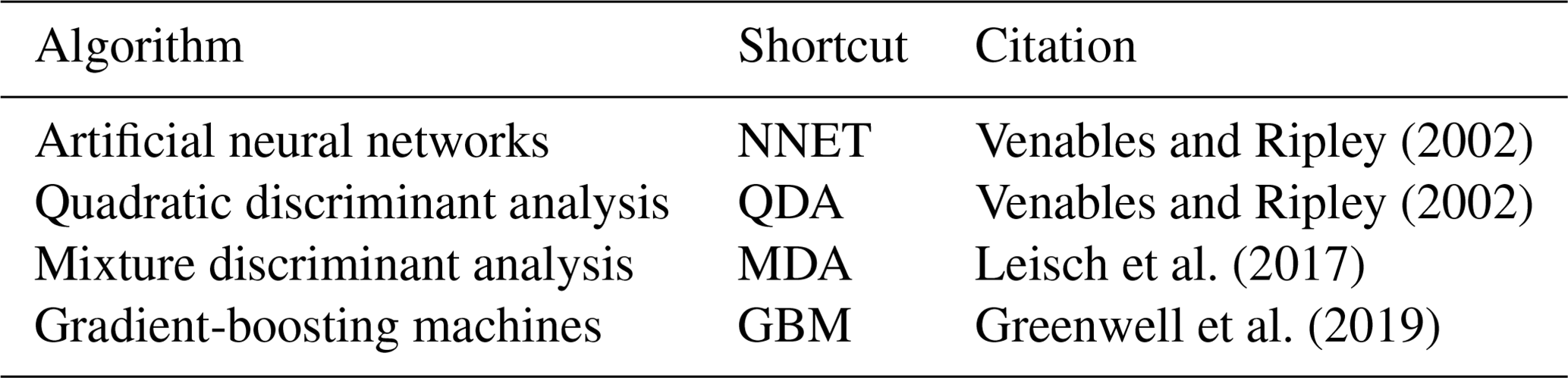
Comparatively simple classification problems arise in this work, so relatively simple artificial neural network (ANN) structures can be used. These deliver similarly good results with significantly less computational cost, and the risk of overfitting is generally lower with simpler structures. After initial tests, the ANN from the nnet package is chosen in this work (NNET). It is a feedforward neural network that allows one hidden layer with an arbitrary number of hidden neurons (Venables and Ripley, 2002).
Discriminant analysis involves the development of discriminants, i.e., linear combinations of independent variables that discriminate the categories of the dependent variable (James et al., 2013). QDA, for example, extracts discriminants that maximize separation between groups and then uses them to perform a Gaussian classification. QDA accounts for heterogeneity in the covariance matrices of these groups. Mixture discriminant analysis (MDA) can be regarded as an extension that modifies the within-group multivariate density of predictors by a mixture (i.e., a weighted sum) of multivariate normal distributions (Rausch and Kelley, 2009).
Gradient-boosting machines (GBM) is chosen to introduce an ML algorithm based on decision trees. It is a generalization of tree-boosting that attempts to mitigate the following problems: speed; interpretability; robustness to overlapping group distributions; and, most importantly, mislabeling of the training data (Hastie et al., 2009). Thus, it creates an accurate and effective standard procedure.
The approach presented here to systematically identify the most appropriate method to describe the relationship between botanical data and climate remedies the last disadvantage mentioned in the introduction.
This section first presents the results of the machine learning competition. Afterwards, the reconstruction of Lake Kinneret and the corresponding MCMC data are shown.
4.1 Machine learning competition
In the following, the results of the machine learning competition are analyzed in detail. The evaluation focuses on the problem of unbalanced data sets. These are augmented with SMOTE until the input values are balanced. Subsequently, the models are trained on these data sets and finally evaluated with a fraction of the original data.
In our work, this classification is based on the so-called balanced accuracy (BA), which is calculated using 2×2 contingency tables of predicted data compared to hold-out validation data. From these, the true positive and true negative rates can be calculated, referred to as sensitivity and specificity, respectively (Chicco et al., 2021). The arithmetic mean of these two measures is the BA, which is an appropriate metric for trained ML models designed to describe an unbalanced data set (Brodersen et al., 2010). BA varies between zero and 1, with values close to 1 indicating well-performing classifications.
The results of all trained models are shown in Fig. 5a. A distinction is made between models trained on the original data set (without SMOTE) and those trained on data augmented with SMOTE. It is immediately noticeable that the results marked by the blue boxplots have a BA of ∼0.5 or the sensitivity is always zero and the specificity is 1, which means that no presence is predicted. In contrast, the other fits (orange boxplots) have an average BA of about 0.92, which provides a clear improvement in BA. Thus, we can not only obtain fitted models with high significance but also reduce the boundary effects in the feature space, resulting in more closed probability contour lines as shown in Fig. 5c. Although all four algorithms provide well-trained models on their own (see Fig. 5a), the direct comparison between them leads to the final selection that a simple artificial neural network emerges as the winner. The structure of this NNET is shown in Fig. 5b, where the two climate variables represent the input layer and the three biomes with the unspecified biome represent the output layer. Furthermore, six hidden neurons proved to be the best compromise between BA and overfitting in model-tuning. This network structure is finally used for the following climate reconstruction.
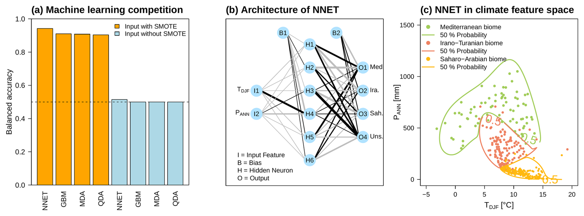
Figure 5Panel (a) summarizes the balanced accuracy of all ML algorithms based on the original input data and the data modified with SMOTE. The winner of this ML competition is the feedforward neural network shown in panel (b). The thickness of the respective lines reflects the relative absolute value of the parameters. Furthermore, the gray lines stand for negative values, and the black lines stand for positive values. In panel (c), the classification in the feature space of TDJF and PANN is shown: the solid colored lines represent the 50 % probability of the biomes occurring based on the transfer function from panel (b). The corresponding original input data are also shown as colored dots.
In summary, the results of the ML competition for estimating the transfer functions between the presence of biomes and their feature space of DJF temperature and the annual sum of precipitation do automate decisions in the interests of reproducibility and, in doing so, raise the quality of transfer function calculations. This introduces a higher flexibility in the case of analyses of a network of proxy data sets, e.g., as a basis for climate field reconstructions.
4.2 Quantitative reconstruction
Due to the large number of parameters and data points, we decided to generate 1 million MCMC samples. This makes the numerical problem difficult to be solved fully in an R (or Python) programming interface. Therefore, as much as possible, subroutines are implemented in the compiler language C and embedded into the R code. With this approach, the reconstruction model can be implemented on a standard laptop or standalone PC with a commercially available standard 8-core central processor and takes about 40–60 s to generate the MCMC samples and perform their evaluation.
Firstly, the stochastic behavior of this MCMC simulation must be tested for convergence. For this, we use the multivariate extension of the Gelman–Rubin convergence indicator (Brooks and Gelman, 1998). The closer this is to 1, the more likely it is that convergence has been achieved. Gelman et al. (2013) recommend a value of less than 1.1. In our case, this is 1.001, from which we conclude that this simulation setup converges.
Figure 6 summarizes the posterior taxa weights ℙ(P∣vecω) determined by this simulation in boxplots. It is immediately apparent that, with the exception of Olea europaea, Quercus calliprinos and Q. ithaburensis, and Amaranthaceae, the mean posterior taxa weights deviate only slightly from the prior uniform distribution. In particular, the olive taxon receives a considerably lower weight, which is due to the generally high pollen percentage in the core (see Appendix B for details). To ensure a sufficiently high variability with respect to the reference curve of AP percentage in Fig. 3b, the new reconstruction method weights Quercus calliprinos and Amaranthaceae the highest, especially under the prior R2=0.5.

Figure 6Posterior and prior taxa weights. The continuous solid black line indicates the prior, and the boxplots indicate the posterior. The short black line and the colored dots within each boxplot indicate the median weight under the explained variance mean values of 0.5, 0.25 (turquoise), and 0.75 (orange). The latter vary clearly only for Olea europaea and the two Quercus taxa. In addition, the assignment of each taxon to the three biomes is color-coded.
Figure 7 shows the prior and posterior probability distributions based on the NNET classification under SMOTE. We see the largest changes from prior to posterior within the Mediterranean biome in Fig. 7a but almost no changes in the posterior between the imposed explained variances R2=0.25, 0.5, and 0.75. The branch with lower temperature and precipitation of this distribution leads to reconstructions that cannot fulfill the CRU-imposed boundary conditions with respect to temperature. The corresponding posterior probability reveals an average TDJF of 10 °C and a PANN of 700 mm. For the two remaining biomes, the changes between prior and posterior and the changes within the three posterior with the different imposed explained variances R2=0.25, 0.5, and 0.75 are minor. The results for the three other classification algorithms are of a similar structure. In Fig. 7d, we see the reduced posterior variances over the prior variance in the climate variables within the biomes due to the ingestion of the additional information of the reference curve and the CRU climate. The temperature distribution of the Saharo-Arabian biome, for example, must be constrained so that it does not contradict the CRU boundary conditions of the most recent temperature data. Overall, it can be seen that the posterior temperatures settle at around 10 °C and thus show less variability than the corresponding precipitation distribution.
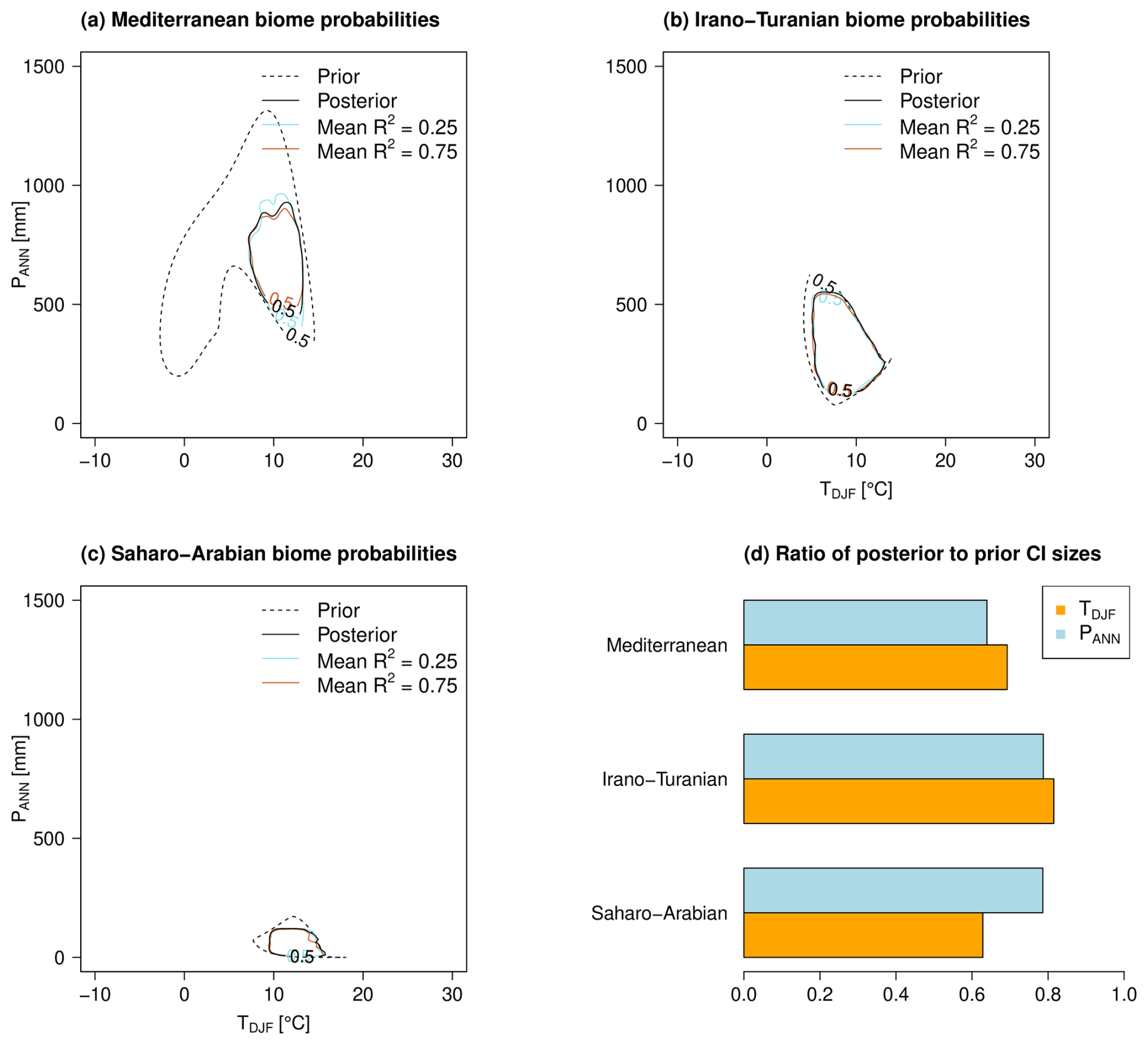
Figure 7In panels (a)–(c), the prior biome probabilities of 50 % are indicated with dashed black lines and the corresponding posterior biome probabilities are depicted with solid black lines for the case of explained variance R2=0.5 by the reference arboreal pollen percentage, and they are depicted in color (turquoise and orange) for R2=0.25 and 0.75. In panel (d), the ratios of the 95 % credible interval (CI) of the corresponding prior and posterior distributions from panels (a)–(c) for the R2=0.5 case are shown.
The posterior samples described above are determined with the prior boundary conditions in Fig. 8. We also see the corresponding posterior distributions as gray areas for the case R2=0.5. It is noticeable that the temperature in Fig. 8a and the precipitation in Fig. 8b have slightly smaller maximum values but that the changes from prior to posterior are mainly visible in the spread around the maximum, corresponding to the results in Fig. 7d. In contrast, the largest changes from prior to posterior are found in the explained variances in the arboreal pollen percentage curve in Fig. 8c. Based on the taxa weights and the values of the transfer functions from Figs. 6 and 7, it can be concluded that a trade-off with respect to recent climate conditions is reached when the median R2 is around 0.65 (50 % CI from 0.50 to 0.80), which is reached with the prior choice of beta distribution with maximum and mean at R2=0.5. In contrast to the prior choice, R2=0.25 and 0.75, this leaves enough degrees of freedom to increase the posterior to 0.65 (50 % CI from 0.50 to 0.80), which does not happen that clearly with the two remaining choices.
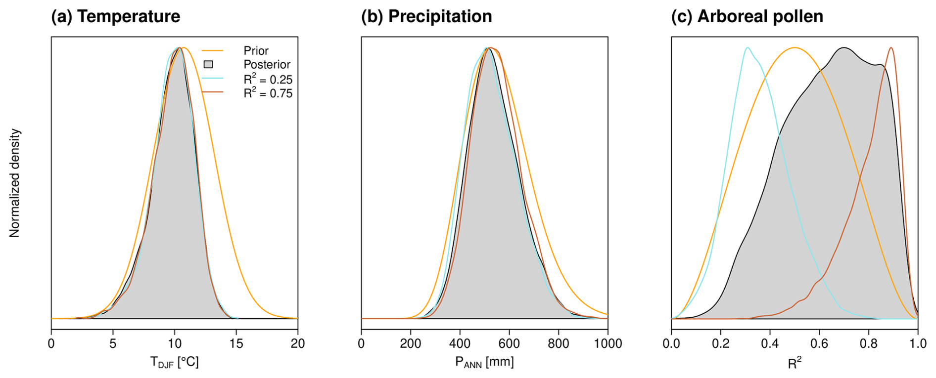
Figure 8The prior proposal distributions (orange lines) and the posterior samples (gray areas for R2=0.5; turquoise and brown lines for R2=0.25 and 0.75) of (a) TDJF, (b) PANN, and (c) the explained variance R2 in the reconstructions when compared to the arboreal pollen percentage reference curve with the three different explained variances R2=0.25, 0.5, and 0.75.
In the following, we describe the final reconstruction. It is divided into the percentages of the reconstructed biomes in Fig. 9 and the reconstructed TDJF and PANN in Fig. 10. From the former, we can infer the importance of these biomes in specific periods.
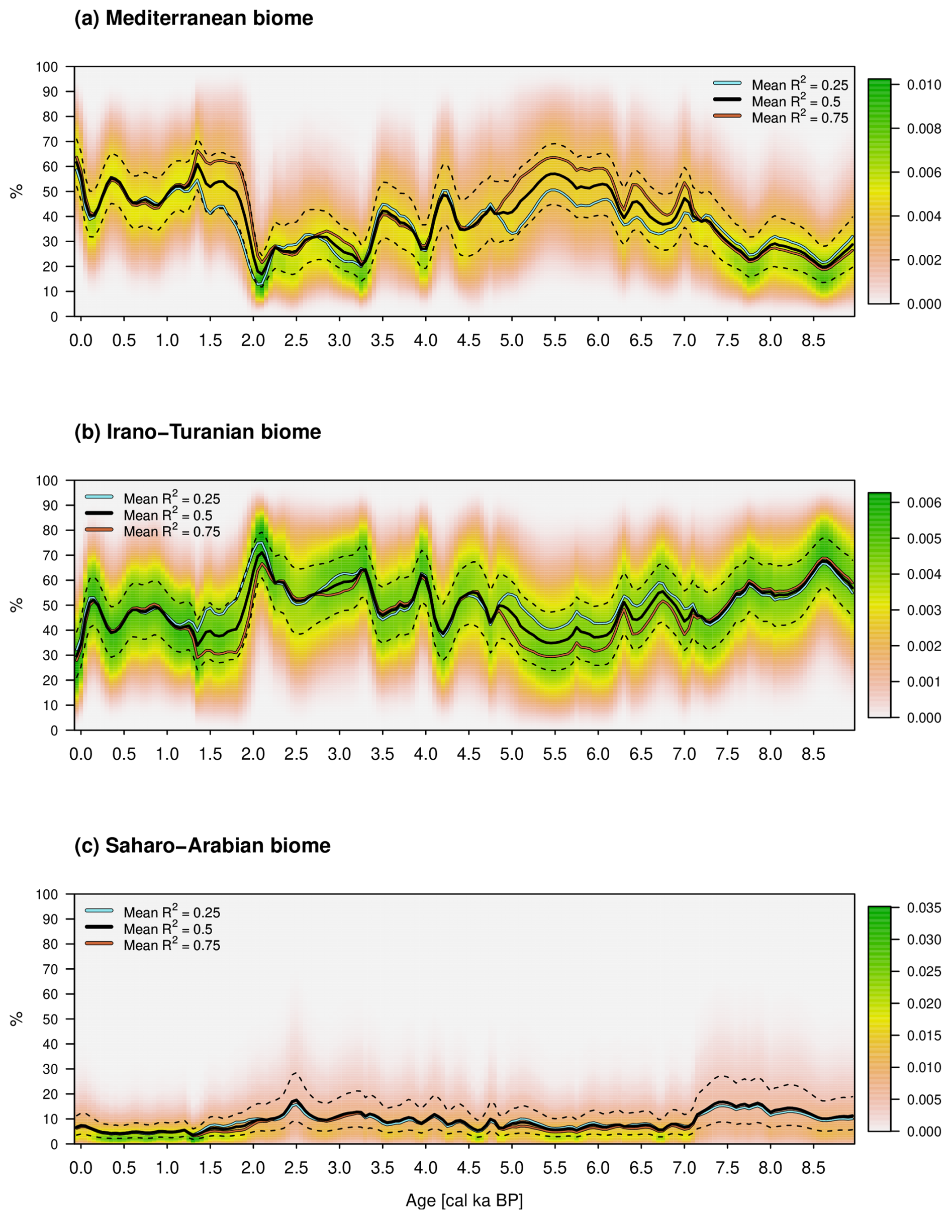
Figure 9Posterior biome percentages in relation to cal ka. The colors indicate the probability density values, the solid black lines indicate the median for the reconstruction based on the explained variance R2=0.5 by the AP percentage, and the dashed black lines indicate the first and third quartiles. The turquoise and brown lines are the medians for R2=0.25 and 0.75.
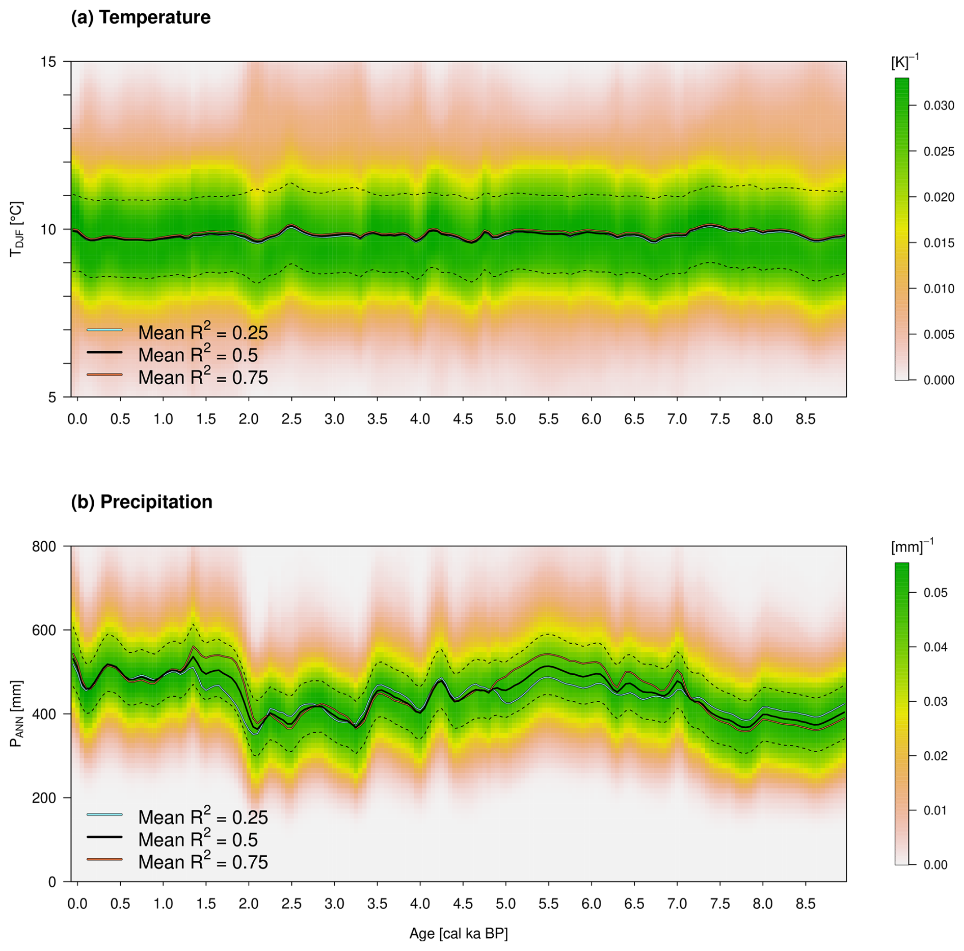
Figure 10As in Fig. 9 but for the quantitative paleoclimate reconstruction of the Lake Kinneret region. (a) The reconstructed TDJF in degrees Celsius (°C). (b) The PANN in millimeters (mm).
The period 9–7 cal ka BP can be associated mainly with the Pottery Neolithic. The vegetation is described in Schiebel and Litt (2018) with a strong influence of steppe vegetation in the catchment area of LK. They conclude that this is due to increasing drought, which is confirmed by the increased percentages of the Saharo-Arabian and Irano-Turanian biomes. In contrast, the Mediterranean biome records comparatively low percentages during this period. This leads on the one hand to the highest average TDJF of over 10 °C and, on the other hand, to a relatively low PANN of about 400 mm. Furthermore, Miebach et al. (2022) infer a weak cooling trend and precipitation decrease during 7.8–6.6 cal ka BP from carbon isotope signals of the Sea of Galilee. These qualitative statements are confirmed by the new climate reconstruction within both variables.
The beginning of the period 7–5 cal ka BP is accompanied by an increase in Olea europaea and thus the Mediterranean biome. Schiebel and Litt (2018) assume climate change towards higher precipitation compared to the previous time slice (9–7 cal ka BP). In addition, Hazan et al. (2005) and Vossel et al. (2018) describe a high Kinneret lake level during the Chalcolithic and Early Bronze Age, which is also confirmed by our reconstruction. This change is well accompanied by the changes in the median position when varying the prior explained variance by the AP percentage reference curve, which is hardly visible, e.g., for the early period 9–7 cal ka BP.
The average PANN is about 500 mm and temperatures surrounding 10 °C. During the Chalcolithic (ca. 6.5–5.5 cal ka BP), precipitation shows a local maximum, which decreases after about 5.5 cal ka BP. Such behavior could be related to the transition from the Chalcolithic to the Early Bronze Age.
The Early Bronze Age to Iron Age within 5–2.3 cal ka BP reflects not only human-induced but also climatically driven vegetation changes with almost no differences between the medians of the three sensitivity calculations based on the prior choices of explained variances R2=0.25, 0.5, and 0.75. On the one hand, the decrease in oak pollen of 4 and 3.2 cal ka BP could be related to the Bond events of 4.2 and 3.2 associated with droughts in the Levant. During this period, the precipitation shows a steady decline from ca. 500 mm to about 400 mm, while the temperature remains around 10 °C. On the other hand, Schiebel and Litt (2018) describe the end of olive cultivation around 5 cal ka BP as a human influence. Therefore, a decrease in olive pollen around 5 cal ka BP cannot be associated with changed climatic conditions and is also not visible in the reconstruction. This is made possible by the lower weighting of this taxon and supports the choice of the prior beta distribution parameters of R2=0.5. Olea europaea is an integral part of the Mediterranean vegetation zone, even as an indicator species for the current geobotanical distribution of this biome (Langgut et al., 2013). Olea also grows as a cultivated tree mainly under Mediterranean climate conditions. When olive groves were planted in the past, the Mediterranean oak forests, which were predominantly deciduous, had to be cleared (e.g., Q. ithaburensis). Oak trees were therefore replaced by olives and vice versa (see Fig. 6). Both species have a similar chance of being recorded in the pollen record (high pollen producer based on wind pollination). It is also noteworthy that the bivariate conditional probability density functions (likelihood functions) of December–January–February temperature and annual precipitation are very similar for both species (see Neumann et al., 2007). The subfamilies Cichorioideae and Asteroideae (both belonging to the Asteraceae family) are components of the Irano-Turanian steppe vegetation. They might also occur in the anthropogenic-influenced Mediterranean vegetation zone (batha, garrigue). However, it must be stressed that the Cichorioideae peaks appear in a phase which was less influenced by human impact (Middle Bronze Age after the decrease in Olea cultivation and increase in Q. ithaburensis type). Therefore we assume a stronger climate than anthropogenic signal related to Cichorioideae peaks (dryer conditions).
Between 4 and 3.2 cal ka BP, the Mediterranean biome apparently decreases and the others increase. The climate change to lower precipitation around 4 cal ka BP could be related to the transition from the Early to the Middle Bronze Age. The second and larger variation during 3.2 cal ka BP might be related to the collapse of the Late Bronze Age (Langgut et al., 2013). Furthermore, the Iron Age in the Near East lasted from about 3.1–2.5 cal ka BP (Langgut et al., 2013). This corresponds to an increase in precipitation at the beginning and ends in a minimum with values around 400 mm. The transition from the Iron Age to the Babylonian–Persian period is marked by 2.5 cal ka BP and lasted about 200 years, accompanied by a slight increase in precipitation.
The years from 2.3–1.5 cal ka BP are marked by the Hellenistic and Roman–Byzantine periods. This can be associated with the Roman Climatic Optimum (Langgut et al., 2013), and a noticeable increase in precipitation can be seen in the reconstruction. Orland et al. (2009) recognize from isotopic data from Soreq Cave a decrease in precipitation during the period 1.9–1.3 cal ka BP. They suggest that this climate change weakened the economic system of the Roman and Byzantine empires, which contributed to the decline in their rule in the Levant.
This leads us to the early Islamic period to the present, from 1.5–0 cal ka BP. The reconstructed PANN shows relatively high values and exhibits only minor variations. Finally, the climate PDFs of the youngest time slice are the same as the posterior distributions depicted in Fig. 8a and b.
In comparison with the quantitative climate reconstruction of the Dead Sea in Fig. 11, we can observe some similarities. During the early Holocene, relatively low precipitation is reconstructed up to 6.5 cal ka BP. These increase markedly during the mid-Holocene up to 3.3 cal ka BP. They then fall significantly and rise in the further course until the youngest time slice. With the corresponding TDJF, the trend is exactly the opposite. Overall, we see similar patterns, although the temperature fluctuations in Litt et al. (2012) are larger, which is due to the special location of the Dead Sea as a transition zone of the three biomes.

Figure 11Paleoclimate reconstruction of the Dead Sea, modified after Litt et al. (2012). (a) The TDJF anomaly in degrees Celsius (°C). (b) The PANN in millimeters (mm). The thicker white lines are the expectation values, and the thinner white lines describe the respective linear climate trends. The thicker black lines mark the mode, and the thinner black lines indicate the interdecile and interquartile ranges.
Note that the presented method and that of Litt et al. (2012) reconstruct a full probability density PDF of the joint Dec–Jan–Feb mean temperature and the annual precipitation sum at a given age. The apparent smoothness of the Dec–Jan–Feb mean temperature in Fig. 10a results if one concentrates on the median of the reconstructed PDF without considering the inherent variability indicated by the color-shading. The median temperature is the temperature value that divides the reconstructed temperature range into two equal probable intervals from which individual realization of the DJF temperatures has to be drawn at random. This randomization introduces additional variability in the time series but requires the specification of the autocorrelation in time beyond that which is introduced by the AP percentage reference curve. The effects of such randomization in the climate field reconstruction of Holocene temperature in Europe have been demonstrated by Simonis et al. (2012). The comparison of the present reconstruction with other temperature reconstruction, e.g., based on non-pollen data, can only be done if these two types of information (the most probable or median value plus the implied variability) are quantitatively available (see Gneiting and Raftery, 2007).
Our new approach of a local climate reconstruction offers a systematic method to investigate the variability in the data under certain boundary conditions. These partly originate from sources other than the original botanical proxy data. In this way, it can be determined whether a physically and biologically realistic climate reconstruction is possible with the given proxy data. The new method shows, for example, that the probability of the Mediterranean biome with lower temperatures and precipitation in Fig. 7a cannot be used when constrained by recent climate data and arboreal pollen reference. So far, the full distributions have been included in the reconstructions. This new flexibility in terms of transfer functions accounts for the assumption that the relationship between recent biome distributions and the corresponding climate remains unchanged in space and time. The posterior distributions in Fig. 9 show where these might have been on average during the reconstruction period for the Sea of Galilee.
Further useful information can be obtained from the posterior taxa weights. From this, it can be deduced to what extent a particular taxon is included in the reconstruction based on its occurrence in the sediment core. Thus, this automatically determined data can expand the underlying expert knowledge. Here it seems that less weight needs to be given to olive pollen, which dominates at certain depths, to ensure the influence of the other taxa. This shows how the highest possible variability can be obtained from the proxy information under the assumed boundary conditions. With a comparatively higher weighting of Quercus calliprinos, the recent precipitation distribution at the Sea of Galilee can be approximated as well as possible. Furthermore, we find the highest weights in relation to the Irano-Turanian and Saharo-Arabian biomes in the taxa Poaceae and Amaranthaceae. This makes it possible to reconstruct the lower precipitation in the periods 9–7 and 3.2–2 cal ka BP. It also helps to reduce the human impact on vegetation during the reconstruction process. This is particularly striking in the Mediterranean biome around 5 cal ka BP, where we see only minor changes.
In the posterior distribution of the explained variance between the reconstructed precipitation and AP percentage in Fig. 8c, values of 0.65 occur on average starting from the prior information that the mean R2=0.5 with an assumed uncertainty of ±0.2. These relatively high positive posterior correlations confirm the relationship between these two variables proposed in Schiebel and Litt (2018) and allow the quantitative exploration of that proposal. We also see the order of magnitude in which this must be present to allow a compromise with the other boundary conditions in Fig. 8a and b.
Compared to previous local climate reconstructions based on Bayesian statistics, the proxy information considered can be included without further processing. This means that it is not necessary to pre-select specific plant data and set thresholds for their probability of occurrence. In addition, the boundary conditions, such as climate anchor points and reference curves, can be extended. For example, isotope data from the Mediterranean Sea, such as MEDSTACK (Colleoni et al., 2012), or from speleothems in the Soreq Cave (Bar-Matthews et al., 2003) can be used as guidelines. In addition, PDFs for the MH from paleoclimate simulations (Braconnot et al., 2011) can be included. The new reconstruction method can therefore be easily adapted and used accordingly in future studies.
The age uncertainty accounted for in this study with the new age–depth transformation presented allows data-driven smoothing and stretching/compressing of the original depth axis of the proxy information, as well as arbitrarily high resolution and a regular temporal grid. This means that reference proxies can now be examined in spectral space. For example, the fluctuations around 4 and 3.2 cal ka BP could be compared with the ice-rafted debris of the North Atlantic using wavelet power spectra (Debret et al., 2007). We thus see that the reconstruction method presented can be extended with additional independent proxy information, so that quantitative multiproxy analyses and the inclusion of results from paleoclimate simulations are possible.
In this study, we present new techniques for generating local paleoclimate reconstructions based on botanical proxies. For this purpose, we use a newly developed BHM solved with MCMC sampling. To place the proxy information in a temporal context, a new probabilistic method is used to assign age information to depths in sediment cores. In particular, the uncertainty of age is accounted for by a separate BHM introduced in this work. Climate variables, such as TDJF and PANN, were included using a transfer function based on biome occurrence. We determine these functions with a machine learning competition. Such a systematic identification of the most appropriate method to describe the relationship between botanical data and climate is performed here for the first time.
These new techniques are applied to plant data from the Sea of Galilee during the Holocene. The reconstructed climate variables reflect the qualitative climate reconstructions explained in Schiebel and Litt (2018), Miebach et al. (2022), and Orland et al. (2009). Moreover, the algorithm is able to find climate changes that can be associated with Bond events and known archeological and cultural changes in the Levant. Furthermore, there is a connection with the quantitative reconstruction of the Dead Sea in Litt et al. (2012), where similar climatological trends are reconstructed. It is interesting to note that the reconstructed Dead Sea lake-level curve as an independent proxy for precipitation (Stein et al., 2010) correlates very well with the pollen-based paleoclimate reconstruction (Litt et al., 2012). However, it must be stressed that the older reconstruction method based on a Bayesian biome model has some weaknesses compared to the new approach which are not detectable by the correlation, namely systematic shifts (biases) with respect to present climate; e.g., the mean Dec–Jan–Feb temperature in Litt et al. (2012) is clearly too low due to the inclusion of temperature values of the Mediterranean vegetation zone in the northern part of the study area.
Overall, our new methods provide an additional way to calculate quantitative paleoclimate reconstructions. From our results, we conclude that more automatic, statistics-based techniques complement those that require additional assumptions. Furthermore, our model provides additional information, such as taxa weights and biome climate ranges with corresponding uncertainty estimates. From this, we can gain new insights into possible biological mechanisms involved in ecological changes caused by past climate variability. The new method not only remedies all the disadvantages mentioned in the Introduction but also represents an attempt to solve complex BHMs with little computational cost. Extending this to multiple proxy sources and applying it to other geographical areas could qualitatively and quantitatively expand knowledge about the climate history of the Earth.
Using Bayes' theorem, we can express the probability distribution for climate C given pollen and macrofossils P, depth D, and parameter Θ. In the process, we also introduce the biome information B:
In the case of a finite number of taxa, the integral is a corresponding sum. Consider in more detail,
with the following assumptions and applications:
-
C is conditionally independent of P if B is given. This assumes that B explains enough variability in the core.
-
The link between C and B is conditionally independent of depth. This means that the relationship between these quantities is assumed to be unchanged for any depth and thus any age of the core. The assumption that this relationship has not changed over time is an important part of our reconstruction method. When we look at older time periods, we need to keep this in mind, as the relationship may well have changed due to evolutionary processes.
-
The connection between C and B is described only by the parameter ψ. Furthermore, ψ and ω are a priori independent: .
-
The application of Bayes' theorem.
If we substitute Eq. (A2) into Eq. (A1), we get
Equation (2) allows us to transform this model from depth to age:
Consider in more detail:
The first term in the integral contains the information about which selected plant proxies Ps from the lake sediment belong to which biome. Note that a more detailed relationship in terms of age A could be added at this point. Because we consider the Holocene in this study, we assume that the probabilities for the biomes are conditionally independent of age if selected plant proxies are given. The second term describes the plant information from the sediment core in terms of age. Finally, we can substitute Eq. (A5) into Eq. (A4) and obtain the reformulated BBM:
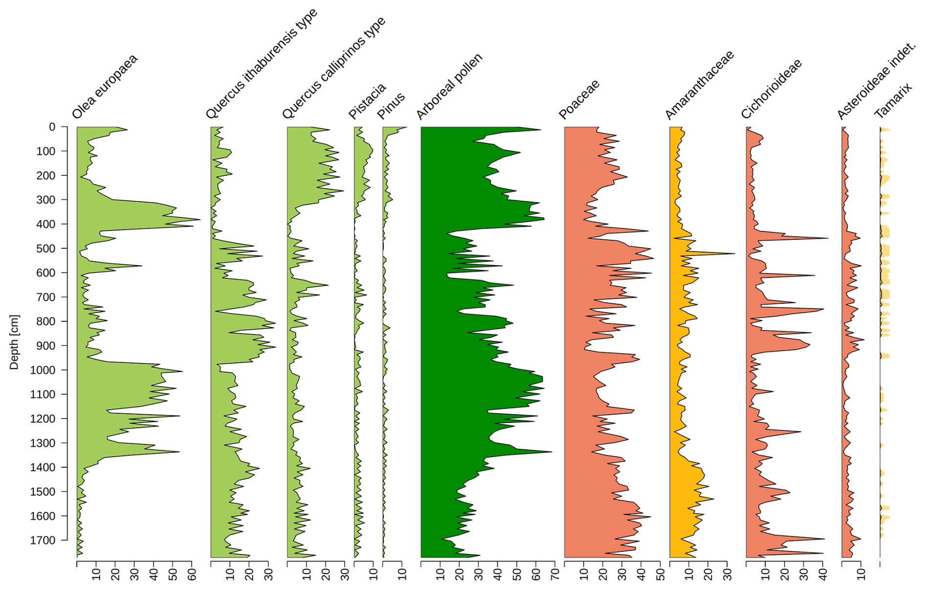
Figure B1Percentage distribution of terrestrial pollen sums as a function of depth for some taxa from the Sea of Galilee. In the middle, the aggregated arboreal pollen is shown in dark green. The other colors correspond to the assignment to the respective biomes.

There are two Zenodo repositories, written in R (Netzel, 2023b) and in Python (Netzel, 2023c). These each include the Bayesian framework with the MCMC simulation in C. The required input data from the sediment core, from the ML competition, and from the age–depth model are available in the corresponding repositories.
TN did the theoretical work, implemented the model and graphics, and wrote most of the text. AM wrote the sections Study area, Material and methods, and Palynology. TL and AM provided the palynological data. AH and TL suggested the reconstruction framework, contributed to the discussion of the results, and commented on the different versions of the paper.
The contact author has declared that none of the authors has any competing interests.
Publisher's note: Copernicus Publications remains neutral with regard to jurisdictional claims made in the text, published maps, institutional affiliations, or any other geographical representation in this paper. While Copernicus Publications makes every effort to include appropriate place names, the final responsibility lies with the authors.
The basic idea and the palynological data for this work were elaborated within the framework of the Collaborative Research Center (SFB) 806 “Our Way to Europe”. We would like to thank Maarten Blaauw for reviewing the Bacon.d.Age function and including it in the rbacon package.
This research has been supported by the Deutsche Forschungsgemeinschaft (DFG project number 57444011).
This open-access publication was funded by the University of Bonn.
This paper was edited by Dominik Fleitmann and reviewed by two anonymous referees.
Bar-Matthews, M., Ayalon, A., Gilmour, M., Matthews, A., and Hawkesworth, C.: Sea-land isotopic relationships from planktonic foraminifera and speleothems in the Eastern Mediterranean region and their implication for paleorainfall during interglacial intervals, Geochim. Cosmochim. Ac., 67, 3181–3199, https://doi.org/10.1016/S0016-7037(02)01031-1, 2003. a
Ben-Avraham, Z., Rosenthal, M., Tibor, G., Navon, H., Wust-Bloch, H., Hofstetter, R., and Rybakov, M.: Structure and Tectonic Development of the Kinneret Basin, in: Lake Kinneret: Ecology and Management, edited by: Zohary, T., Sukenik, A., Berman, T., and Nishri, A., Springer Netherlands, Dordrecht, 19–38, ISBN 978-94-017-8944-8, https://doi.org/10.1007/978-94-017-8944-8_2, 2014. a
Berger, J. O.: Statistical decision theory and Bayesian analysis, Springer Verlag, New York, Berlin, Heidelberg, https://doi.org/10.1007/978-1-4757-4286-2, 2013. a
Berman, T., Zohary, T., Nishri, A., and Sukenik, A.: General Background, in: Lake Kinneret: Ecology and Management, edited by Zohary, T., Sukenik, A., Berman, T., and Nishri, A. Springer Netherlands, Dordrecht, 1–15, ISBN 978-94-017-8944-8, https://doi.org/10.1007/978-94-017-8944-8_1, 2014. a
Beug, H.: Leitfaden der Pollenbestimmung für Mitteleuropa und angrenzende Gebiete, Verlag Dr. Friedrich Pfeil, ISBN 9783899370430, 2004. a
Blaauw, M. and Christen, J. A.: Flexible paleoclimate age-depth models using an autoregressive gamma process, Bayesian Anal., 6, 457–474, https://doi.org/10.1214/11-BA618, 2011. a
Blaauw, M., Christen, J. A., and Aquino L., M. A.: rbacon: Age-Depth Modelling using Bayesian Statistics, R package version 3.3.1, CRAN, https://CRAN.R-project.org/package=rbacon (last access: 23 January 2025), 2020. a
Bowyer, K. W., Chawla, N. V., Hall, L. O., and Kegelmeyer, W. P.: SMOTE: Synthetic Minority Over-sampling Technique, CoRR, abs/1106.1813, arxiv [preprint], https://doi.org/10.48550/arXiv.1106.1813, 2011. a
Braconnot, P., Harrison, S., Otto-Bliesner, B., Abe-Ouchi, A., Jungclaus, J., and Peterschmitt, J.-Y.: The Paleoclimate Modeling Intercomparison Project contribution to CMIP5, CLIVAR Exchanges, 56, 15–19, 2011. a
Brodersen, K. H., Ong, C. S., Stephan, K., and Buhmann, J.: The Balanced Accuracy and Its Posterior Distribution, in: 2010 20th International Conference on Pattern Recognition, 23–26 August 2010, Istanbul, Turkey, 3121–3124, https://doi.org/10.1109/ICPR.2010.764, 2010. a
Brooks, S. and Gelman, A.: General Methods for Monitoring Convergence of Iterative Simulations, J. Comput. Graph. Stat., 7, 434–455, https://doi.org/10.1080/10618600.1998.10474787, 1998. a
Chicco, D., Warrens, M., and Jurman, G.: The Matthews correlation coefficient (MCC) is more informative than Cohen's kappa and Brier score in binary classification assessment, IEEE Access, 9, 78368–78381, https://doi.org/10.1109/ACCESS.2021.3084050, 2021. a
Colleoni, F., Masina, S., Negri, A., and Marzocchi, A.: Plio–Pleistocene high–low latitude climate interplay: A Mediterranean point of view, Earth Planet. Sc. Lett., 319-320, 35–44, https://doi.org/10.1016/j.epsl.2011.12.020, 2012. a
Dan, J., Yaalon, D., Koyumdjisky, H., and Raz, Z.: The Soil Association Map of Israel (1:1 000 000), Israel J. Earth Sci., 2, 29–49, 1972. a
Danin, A.: Flora and vegetation of Israel and adjacent areas, in: The zoogeography of Israel, chap. 7, edited by: Yom Tov, Y. and Tchernov, E., Junk Publishers, Dordrecht, 129–159, ISBN 9061936500, 1988. a
Danin, A.: Flora and vegetation of Israel and adjacent areas, Bocconea, 3, 18–42, 1992. a
Debret, M., Bout-Roumazeilles, V., Grousset, F., Desmet, M., McManus, J. F., Massei, N., Sebag, D., Petit, J.-R., Copard, Y., and Trentesaux, A.: The origin of the 1500-year climate cycles in Holocene North-Atlantic records, Clim. Past, 3, 569–575, https://doi.org/10.5194/cp-3-569-2007, 2007. a
Faegri, K. and Iversen, J.: Textbook of Pollen Analysis, Wiley, ISBN 9780471921783, 1989. a
Gebhardt, C., Kühl, N., Hense, A., and Litt, T.: Reconstruction of Quaternary temperature fields by dynamically consistent smoothing, Clim. Dynam., 30, 421–437, https://doi.org/10.1007/s00382-007-0299-9, 2008. a
Gelman, A., Carlin, J., Stern, H., Dunson, D., Vehtari, A., and Rubin, D.: Bayesian Data Analysis, in: 3rd Edn., Chapman & Hall/CRC Texts in Statistical Science, Taylor & Francis, ISBN 9781439840955, 2013. a, b
Gneiting, T. and Raftery, A. E.: Strictly proper scoring rules, prediction, and estimation, J. Am. Stat. Assoc., 102, 359–378, 2007. a
Greenwell, B., Boehmke, B., Cunningham, J., and Developers, G.: gbm: Generalized Boosted Regression Models, R package version 2.1.5, CRAN, https://CRAN.R-project.org/package=gbm (last access: 23 January 2025), 2019. a
Harris, I., Osborn, T., Jones, P., and Lister, D.: Version 4 of the CRU TS monthly high-resolution gridded multivariate climate dataset, Sci. Data, 7, 109, https://doi.org/10.1038/s41597-020-0453-3, 2020. a
Hastie, T., Tibshirani, R., and Friedman, J.: The Elements of Statistical Learning: Data Mining, Inference, and Prediction, in: Springer series in statistics, Springer, ISBN 9780387848846, 2009. a
Hazan, N., Stein, M., Agnon, A., Marco, S., Nadel, D., Negendank, J. F., Schwab, M. J., and Neev, D.: The late quaternary limnological history of Lake Kinneret (Sea of Galilee), Israel, Quatern. Res., 63, 60–77, 2005. a, b
Hoens, T. R. and Chawla, N. V.: Imbalanced Datasets: From Sampling to Classifiers, in: chap. 3, John Wiley and Sons, Ltd, 43–59, ISBN 9781118646106, https://doi.org/10.1002/9781118646106.ch3, 2013. a, b
James, G., Witten, D., Hastie, T., and Tibshirani, R.: An Introduction to Statistical Learning: with Applications in R, Springer, https://www.statlearning.com/ (last access: 12 October 2019), 2013. a, b
Jergensen, G. E., McGovern, A., Lagerquist, R., and Smith, T.: Classifying Convective Storms Using Machine Learning, Weather Forecast., 35, 537–559, https://doi.org/10.1175/WAF-D-19-0170.1, 2020. a
Kühl, N. and Litt, T.: Quantitative time series reconstruction of Eemian temperature at three European sites using pollen data, Veget. Hist. Archaeobot., 12, 205–214, https://doi.org/10.1007/s00334-003-0019-2, 2003. a
Kühl, N., Gebhardt, C., Litt, T., and Hense, A.: Probability Density Functions as Botanical-Climatological Transfer Functions for Climate Reconstruction, Quatern. Res., 58, 381–392, https://doi.org/10.1006/qres.2002.2380, 2002. a
Kuhn, M., with contributions from Jed, W., Weston, S., Williams, A., Keefer, C., Engelhardt, A., Cooper, T., Mayer, Z., Kenkel, B., the R Core Team, Benesty, M., Lescarbeau, R., Ziem, A., Scrucca, L., Tang, Y., Candan, C., and Hunt., T.: caret: Classification and Regression Training, R package version 6.0-84, CRAN, https://CRAN.R-project.org/package=caret (last access: 22 January 2025), 2019. a
Langgut, D., Finkelstein, I., and Litt, T.: Climate and the Late Bronze Collapse: New Evidence from the Southern Levant, Tel Aviv, 40, 149–175, https://doi.org/10.1179/033443513X13753505864205, 2013. a, b, c, d, e
Leisch, F., Hornik, K., and Ripley., B. D.: mda: Mixture and Flexible Discriminant Analysis, r package version 0.4-10, CRAN, https://CRAN.R-project.org/package=mda (last access: 22 January 2025), 2017. a
Litt, T., Ohlwein, C., Neumann, F. H., Hense, A., and Stein, M.: Holocene climate variability in the Levant from the Dead Sea pollen record, Quaternary Sci. Rev., 49, 95–105, https://doi.org/10.1016/j.quascirev.2012.06.012, 2012. a, b, c, d, e, f, g, h, i, j, k, l
Miebach, A., Niestrath, P., Roeser, P., and Litt, T.: Impacts of climate and humans on the vegetation in northwestern Turkey: Palynological insights from Lake Iznik since the Last Glacial, Clim. Past, 12, 575–593, https://doi.org/10.5194/cp-12-575-2016, 2016. a
Miebach, A., Stolzenberger, S., Wacker, L., Hense, A., and Litt, T.: A new Dead Sea pollen record reveals the last glacial paleoenvironment of the southern Levant, Quaternary Sci. Rev., 214, 98–116, https://doi.org/10.1016/j.quascirev.2019.04.033, 2019. a, b
Miebach, A., Power, M., Resag, T., Netzel, T., Colombaroli, D., and Litt, T.: Changing fire regimes during the first olive cultivation in the Mediterranean Basin: New high-resolution evidence from the Sea of Galilee, Israel, Global Planet. Change, 210, 103774, https://doi.org/10.1016/j.gloplacha.2022.103774, 2022. a, b, c, d, e
Moore, P., Webb, J., and Collinson, M.: Pollen Analysis, Blackwell scientific publications, Blackwell Scientific Publications, ISBN 9780632021765, 1991. a
Netzel, T.: Quantitative paleoclimate reconstructions in the European region based on multiple proxies, PhD thesis, Rheinische Friedrich-Wilhelms-Universität Bonn, https://hdl.handle.net/20.500.11811/10758 (last access: 22 January 2025), 2023a. a, b
Netzel, T.: Reconstruction tools in R, Zenodo [code], https://doi.org/10.5281/zenodo.8214297, 2023b. a
Netzel, T.: Reconstruction tools in Python, Zenodo [code], https://doi.org/10.5281/zenodo.8214290, 2023c. a
Neumann, F., Schölzel, C., Litt, T., Hense, A., and Stein, M.: Holocene vegetation and climate history of the northern Golan heights (Near East), Veget. Hist. Archaeobot., 16, 329–346, https://doi.org/10.1007/s00334-006-0046-x, 2007. a, b, c, d
Orland, I., Bar-Matthews, M., Kita, N., Ayalon, A., Matthews, A., and Valley, J.: Climate deterioration in the Eastern Mediterranean as revealed by ion microprobe analysis of a speleothem that grew from 2.2 to 0.9 ka in Soreq Cave, Israel, Quatern. Res., 71, 27–35, https://doi.org/10.1016/j.yqres.2008.08.005, 2009. a, b, c
Panagiotopoulos, K., Aufgebauer, A., Schäbitz, F., and Wagner, B.: Vegetation and climate history of the Lake Prespa region since the Lateglacial, Quatern. Intern., 293, 157–169, https://doi.org/10.1016/j.quaint.2012.05.048, 2013. a
Prentice, I. C., Cramer, W., Harrison, S. P., Leemans, R., Monserud, R. A., and Solomon, A. M.: Special Paper: A Global Biome Model Based on Plant Physiology and Dominance, Soil Properties and Climate, J. Biogeogr., 19, 117–134, 1992. a
Ramsey, C. B.: Bayesian analysis of radiocarbon dates, Radiocarbon, 51, 337–360, 2009. a
Rausch, J. and Kelley, K.: A comparison of linear and mixture models for discriminant analysis under nonnormality, Behav. Res. Meth., 41, 85–98, https://doi.org/10.3758/BRM.41.1.85, 2009. a
R Core Team: R: A Language and Environment for Statistical Computing, R Foundation for Statistical Computing, Vienna, Austria, https://www.R-project.org/ (last access: 22 January 2025), 2018. a
Reille, M.: Pollen et spores d'Europe et d'Afrique du Nord: supplément 2, Laboratoire de Botanique historique et Palynologie, ISBN 9782950717511, 1995. a
Reille, M.: Pollen et spores d'Europe et d'Afrique du Nord: supplément 2, Laboratoire de Botanique historique et Palynologie, ISBN 9782950717528, 1998. a
Reille, M.: Pollen et spores d'Europe et d'Afrique du Nord, in: 2nd Edn., Laboratoire de Botanique historique et Palynologie, ISBN 9782950717535, 1999. a
Schiebel, V. and Litt, T.: Holocene vegetation history of the southern Levant based on a pollen record from Lake Kinneret (Sea of Galilee), Israel, Veget. Hist. Archaeobot., 27, 577–590, https://doi.org/10.1007/s00334-017-0658-3, 2018. a, b, c, d, e, f, g, h, i, j, k, l
Schölzel, C.: Palaeoenvironmental Transfer Functions in a Bayesian Framework with Application to Holocene Climate Variability in the Near East, Bonner Meteorologische Abhandlungen, Rheinische Friedrich-Wilhelms-Universität Bonn, p. 104, https://www.ifgeo.uni-bonn.de/de/medien-inhalte/bonner-meteorologische-abhandlungen_20240222.pdf (last access: 22 January 2025), 2006. a, b, c, d
Seppä, H., Hammarlund, D., and Antonsson, K.: Low-frequency and high-frequency changes in temperature and effective humidity during the Holocene in south-central Sweden: implications for atmospheric and oceanic forcings of climate, Clim. Dynam., 25, 285–297, https://doi.org/10.1007/s00382-005-0024-5, 2005. a
Simonis, D., Hense, A., and Litt, T.: Reconstruction of late Glacial and Early Holocene near surface temperature anomalies in Europe and their statistical interpretation, Quatern. Int., 274, 233–250, https://doi.org/10.1016/j.quaint.2012.02.050, 2012. a, b
Sneh, A., Bartov, Y., Weissbrod, T., and Rosensaft, M.: Geological Map of Israel, , Geological Survey, https://www.gov.il/en/pages/israel-map-1-200k (last access: 22 January 2025), 1998. a
Stein, M., Torfstein, A., Gavrieli, I., and Yechieli, Y.: Abrupt aridities and salt deposition in the post-glacial Dead Sea and their North Atlantic connection, Quaternary Sci. Rev., 29, 567–575, 2010. a, b
Stolzenberger, S.: On the probabilistic evaluation of decadal and paleoclimate model predictions, PhD thesis, Rheinische Friedrich-Wilhelms-Universität Bonn, https://hdl.handle.net/20.500.11811/7299 (last access: 22 January 2025), 2017. a
Thoma, B.: Palaeoclimate Reconstruction in the Levant and on the Balkans, PhD thesis, Rheinische Friedrich-Wilhelms-Universität Bonn, https://hdl.handle.net/20.500.11811/7204 (last access: 22 January 2025), 2017. a, b, c
Torfstein, A., Goldstein, S. L., Kushnir, Y., Enzel, Y., Haug, G., and Stein, M.: Dead Sea drawdown and monsoonal impacts in the Levant during the last interglacial, Earth Planet. Sc. Lett., 412, 235–244, https://doi.org/10.1016/j.epsl.2014.12.013, 2015. a
Venables, W. N. and Ripley, B. D.: Modern Applied Statistics with S, in: 4th Edn., Springer, New York, ISBN 0-387-95457-0, 2002. a, b, c
Vossel, H., Roeser, P., Litt, T., and Reed, J. M.: Lake Kinneret (Israel): New insights into Holocene regional palaeoclimate variability based on high-resolution multi-proxy analysis, Holocene, 28, 1395–1410, 2018. a, b
Weitzel, N., Hense, A., and Ohlwein, C.: Combining a pollen and macrofossil synthesis with climate simulations for spatial reconstructions of European climate using Bayesian filtering, Clim. Past, 15, 1275–1301, https://doi.org/10.5194/cp-15-1275-2019, 2019. a, b, c
Ziv, B., Shilo, E., Lechinsky, Y., and Rimmer, A.: Meteorology, in: Lake Kinneret: Ecology and Management, edited by: Zohary, T., Sukenik, A., Berman, T., and Nishri, A., Springer Netherlands, Dordrecht, 81–96, ISBN 978-94-017-8944-8, https://doi.org/10.1007/978-94-017-8944-8_6, 2014. a
Zohary, M.: Plant Life of Palestine: Israel and Jordan, Chronica botanica, Ronald Press Company, ISBN 9780471068280, 1962. a, b, c, d
Zohary, M.: Vegetation of Israel and Adjacent Areas, Reichert, ISBN 9783882261257, 1982. a, b
- Abstract
- Introduction
- Study area
- Material and methods
- Results
- Discussion and possible extensions
- Conclusions
- Appendix A: Derivation of the local reconstruction model
- Appendix B: Figures of the taxa spectrum
- Code and data availability
- Author contributions
- Competing interests
- Disclaimer
- Acknowledgements
- Financial support
- Review statement
- References