No detectable influence of the carbonate ion effect on changes in stable carbon isotope ratios (δ¹³C) of shallow dwelling planktic foraminifera over the past 160 kyr

Laboratory experiments showed that the isotopic fractionation of δ¹³C and of δ¹⁸O during calcite formation of planktic foraminifera are species-specific functions of ambient CO${}_{\mathrm{3}}^{\mathrm{2}-}$ concentration. This effect became known as the carbonate ion effect (CIE), whose role for the interpretation of marine sediment data will be investigated here in an in-depth analysis of the ¹³C cycle. For this investigation, we constructed new 160 kyr long mono-specific stacks of changes in both δ¹³C and δ¹⁸O from either the planktic foraminifera Globigerinoides ruber (rub) or Trilobatus sacculifer (sac) from 112 and 40 marine records, respectively, from the wider tropics (latitudes below 38°). Both mono-specific time series Δ(δ¹³C_rub) and Δ(δ¹³C_sac) are very similar to each other, and a linear regression through a scatter plot of both data sets has a slope of ∼ 0.99 – although the laboratory-based CIE for both species differs by a factor of nearly 2, implying that they should record distinctly different changes in δ¹³C, if we accept that the carbonate ion concentration changes on glacial–interglacial timescales. For a deeper understanding of the ¹³C cycle, we use the Solid Earth version of the Box model of the Isotopic Carbon cYCLE (BICYLE-SE) to calculate how surface-ocean CO${}_{\mathrm{3}}^{\mathrm{2}-}$ should have varied over time in order to be able to calculate the potential offsets which would by caused by the CIE quantified in culture experiments. Our simulations are forced with atmospheric reconstructions of CO₂ and δ¹³CO₂ derived from ice cores to obtain a carbon cycle which should at least at the surface ocean be as close as possible to expected conditions and which in the deep ocean largely agrees with the carbon isotope ratio of dissolved inorganic carbon (DIC), δ¹³C_DIC, as reconstructed from benthic foraminifera. We find that both Δ(δ¹³C_rub) and Δ(δ¹³C_sac) agree better with changes in simulated δ¹³C_DIC when ignoring the CIE than those time series which were corrected for the CIE. The combination of data- and model-based evidence for the lack of a role for the CIE in Δ(δ¹³C_rub) and Δ(δ¹³C_sac) suggests that the CIE as measured in laboratory experiments is not directly transferable to the interpretation of marine sediment records. The much smaller CIE-to-glacial–interglacial-signal ratio in foraminifera δ¹⁸O, when compared to δ¹³C, prevents us from drawing robust conclusions on the role of the CIE in δ¹⁸O as recorded in the hard shells of both species. However, theories propose that the CIE in both δ¹³C and δ¹⁸O depends on the pH in the surrounding water, suggesting that the CIE should be detectable in neither or both of the isotopes. Whether this lack of role of the CIE in the interpretation of planktic paleo-data is a general feature or is restricted to the two species investigated here needs to be checked with further data from other planktic foraminiferal species.

1 Introduction

For a reconstruction of past changes in the ocean and in the carbon cycle, various variables are measured in microfossils obtained from marine sediment cores. Among the most widely used are the stable carbon and oxygen isotope ratios, δ¹³C and δ¹⁸O, from hard shells of planktic and benthic foraminifera. Since the publication of the first stable isotope time series (Emiliani, 1955) a vast number of stable isotope records have been published and to a large part compiled in the World Atlas of late Quaternary Foraminiferal Oxygen and Carbon Isotope Ratios (Mulitza et al., 2022). One of the fundamental problems with the interpretation of foraminiferal isotope ratios is how and why a stable isotope signal was altered on its way from the seawater to the shell of living foraminifera. Are there vital and other effects necessary to be considered when interpreting the paleo-records (e.g. Bijma et al., 1999; Zeebe et al., 2008; Kimoto, 2015)?

The carbonate ion effect (CIE) is one of these potentially important effects that might alter the isotopic signal. The CIE implies that both δ¹³C and δ¹⁸O measured in hard shells of marine organisms undergo isotopic fractionation during calcite formation with the amplitude of the fractionation, among other factors, being a function of the carbonate ion concentration ([CO${}_{\mathrm{3}}^{\mathrm{2}-}$]) of the surrounding seawater (Spero et al., 1997). The CIE has been found to be species-specific (Spero et al., 1999), ranging from $-\mathrm{4.7}\times {\mathrm{10}}^{-\mathrm{3}}$ ‰ to $-\mathrm{13.0}\times {\mathrm{10}}^{-\mathrm{3}}$ ‰ per µmol kg⁻¹ of [CO${}_{\mathrm{3}}^{\mathrm{2}-}$] for δ¹³C and between $-\mathrm{1.4}\times {\mathrm{10}}^{-\mathrm{3}}$ ‰ and $-\mathrm{4.5}\times {\mathrm{10}}^{-\mathrm{3}}$ ‰ per µmol kg⁻¹ of [CO${}_{\mathrm{3}}^{\mathrm{2}-}$] for δ¹⁸O in four planktic foraminifera. The CIE for δ¹³C has been explained for Orbulina universa, a spinose, symbiont-bearing species, by the pH-related distribution of dissolved inorganic carbon (DIC) into its three species: CO₂, CO${}_{\mathrm{3}}^{\mathrm{2}-}$ and HCO${}_{\mathrm{3}}^{-}$ (Wolf-Gladrow et al., 1999; Zeebe et al., 1999). The CIE on δ¹⁸O is also explained by the CO${}_{\mathrm{3}}^{\mathrm{2}-}$-related varying pH (Zeebe, 1999). These theories, however, were unable to base the full amplitudes found in experiments solely on this effect. The CIE is maybe the most prominent isotopic fractionation effect which has to be considered when interpreting the paleo-records, but others, e.g vital effects and dependency on light, temperature, pressure and shell size, have been put forward (e.g. Spero and Williams, 1988, 1989; Spero et al., 1991; Spero, 1992; Spero and Lea, 1993; Oppo and Fairbanks, 1989). The CIE is found to play a minor role when comparing late Holocene deep-ocean δ¹³C in benthic foraminifera, with δ¹³C of DIC (δ¹³C_DIC) (Schmittner et al., 2017) being responsible for $-\mathrm{2.6}\times {\mathrm{10}}^{-\mathrm{3}}$ ‰ per µmol kg⁻¹ of [CO${}_{\mathrm{3}}^{\mathrm{2}-}$] disturbance in the recorded signal. In a recent study focusing on the benthic species Cibicidoides wuellerstorfi, $-\mathrm{3.0}\times {\mathrm{10}}^{-\mathrm{3}}$ ‰ per µmol kg⁻¹ of [CO${}_{\mathrm{3}}^{\mathrm{2}-}$] has been obtained for the late Holocene (Nederbragt, 2023). Both studies also found in addition to the CIE that δ¹³C_benthic was also partly controlled by other variables, mainly pressure (water depth) and temperature.

The CIE in planktic foraminifera is one of the reasons why the interpretation of the whole δ¹³C cycle over glacial–interglacial timescales is still challenging. In a compilation of foraminiferal δ¹³C measurements covering the past 150 kyr, Oliver et al. (2010) find relatively large disagreements between different planktic δ¹³C records within a region compared to benthic records, consistent with large uncertainty attributed to the estimation of δ¹³C_DIC from planktic species. Since benthic compilations are less affected by the CIE, they should, however, robustly constrain deep-ocean changes in δ¹³C_DIC. A more recent compilation of benthic δ¹³C was given in Lisiecki (2014). Furthermore, δ¹³C of atmospheric CO₂ (δ¹³CO₂) is now available over the last 155 kyr (Eggleston et al., 2016a) from ice cores. So far, tight constraints on the change in surface-ocean δ¹³C_DIC are missing from our understanding, but, in principle, this information should be recorded in the hard shells of planktic foraminifera, even if hidden under the CIE.

In this study, we therefore aim to construct a robust time series of orbital changes in surface-ocean δ¹³C_DIC based on planktic foraminifera data. We compiled δ¹³C data largely based on Mulitza et al. (2022) covering the last 160 kyr. In order to be able to apply any species-specific CIE corrections, we compile mono-specific isotope records on the widely abundant shallow-dwelling planktic foraminifera species Globigerinoides ruber (G. ruber or rub) and Trilobatus sacculifer (T. sacculifer or sac) into stacks. Due to their spatial distribution (Fraile et al., 2008), this species selection leads effectively to the construction of Δ(δ¹³C_rub) and Δ(δ¹³C_sac) stacks based on sediment core data from latitudes smaller than 40°, potentially informing us about mean changes of δ¹³C_DIC on orbital timescales in the surface of the wider tropical ocean. Accompanied stacks of Δ(δ¹⁸O_rub) and Δ(δ¹⁸O_sac) from the same cores will add further information on the CIE in δ¹⁸O.

A first surface-ocean δ¹³C stack based on data from T. sacculifer obtained from five equatorial Atlantic records has been constructed by Curry and Crowley (1987) without any knowledge on the CIE. Furthermore, Spero et al. (1999) used data from G. ruber and T. sacculifer from a single core in the Indian Ocean and the lab-based size of their species-specific CIE to deconvolve surface-ocean [CO${}_{\mathrm{3}}^{\mathrm{2}-}$]. Here we will use our new mono-specific δ¹³C stacks, which, due to the underlying number of records, have a much higher signal-to-noise ratio to test the robustness of their findings.

In the following, we will investigate the connection of δ¹³C in the atmosphere and ocean in closer detail in order to improve our understanding of the ¹³C cycle. The remainder of the article is structured as follows. Firstly (Sect. 2.1), we describe the construction of our mono-specific δ¹³C anomaly stacks, Δ(δ¹³C_rub) and Δ(δ¹³C_sac) (and of the accompanied δ¹⁸O anomalies). Some published benthic δ¹³C data are also needed for our understanding (Sect. 2.2). For a deeper interpretation, the global isotope-enabled carbon cycle model, the Solid Earth version of the Box model of the Isotopic Carbon cYCLE (BICYCLE-SE) (Köhler and Munhoven, 2020), which has been proven to simulate glacial–interglacial (G-IG) in the carbon cycle reasonably well, is used. The model is briefly described in Sect. 2.3, including a completely revised parametrisation of the ¹³C cycle. In Sect. 3.1, we discuss what we already know from data on the δ¹³C cycle and the role the CIE might play. We then analyse the simulated δ¹³C cycle in our model results in Sect. 3.2. This enables us to evaluate (Sect. 3.3) if our stacks, Δ(δ¹³C_rub) and Δ(δ¹³C_sac), are good representations of changes in δ¹³C_DIC in the wider tropical surface ocean or if corrections such as the CIE need to be applied. Finally, we briefly discuss the CIE in δ¹⁸O_rub and δ¹⁸O_sac (Sect. 3.4) before we come to our conclusions (Sect. 4).

2 Methods

2.1 Constructing new mono-specific stacks from planktic foraminifera

2.1.1 Data source and age modelling

To construct time series of low-latitude δ¹³C variations through the past 160 kyr, we selected 112 and 40 δ¹³C records of the shallow-dwelling planktic foraminifera G. ruber and T. sacculifer, respectively, predominantly from the World Atlas of late Quaternary Foraminiferal Oxygen and Carbon Isotope Ratios (Mulitza et al., 2022). A list of the isotope records contributing to our stacks with relevant metadata, references to the original publications and data sources is provided in Table S1. All data citations are summarized in a condensed way in Appendix A. In three sediment cores, time series from both G. ruber (white) and G. ruber (pink) contribute to our G. ruber stacks, while data from 22 cores contain mono-specific data from both G. ruber and T. sacculifer. All combined, our data selection is based on material from 127 sediment cores. The core sites cover a latitudinal range from 37.6° N to 36.7° S for G. ruber and from 32.8° N to 31.3° S for T. sacculifer in all major ocean basins (Fig. 1), although the contributions from individual cores (and therefore the latitudinal range) changed over time (Fig. 2c). Our age models are based on either radiocarbon ages or oxygen isotope stratigraphy or a combination of both methods. To calibrate radiocarbon ages, we first subtracted a simulated local reservoir age from the nearest grid box of the modelling experiments conducted for Marine20 (Butzin et al., 2020; Heaton et al., 2020a) and then calibrated the corrected radiocarbon age with the IntCal20 calibration curve (Reimer et al., 2020). For core sections with insufficient radiocarbon coverage or outside the radiocarbon dating range, ages were added through the visual alignment with the isotope stacks by Lisiecki and Raymo (2005) and Lisiecki and Stern (2016) using the software PaleoDataView (Langner and Mulitza, 2019). In a few cases, age models were derived by visual alignment with the oxygen isotope records of well-dated nearby cores. The details of the age model construction are available in the netCDF files of the age models in the corresponding PaleoDataView collection (Köhler and Mulitza, 2023). A continuous age model was then constructed with the age modelling software BACON (Blaauw and Christen, 2011). For each record, we produced an ensemble of 1000 time series by combining 1000 BACON-generated age models with 1000 down-core δ¹³C and δ¹⁸O series by adding a random value within the typical analytical 1σ-uncertainty of 0.05 % and 0.07 ‰ to each down-core δ¹³C and δ¹⁸O value, respectively. The resulting 1000 δ¹³C and δ¹⁸O time series were then interpolated to a time step of 1 kyr to calculate the mean and the standard deviation of the time series ensembles. The averaging of the individual ensemble members led to a considerable smoothing of the final time series.

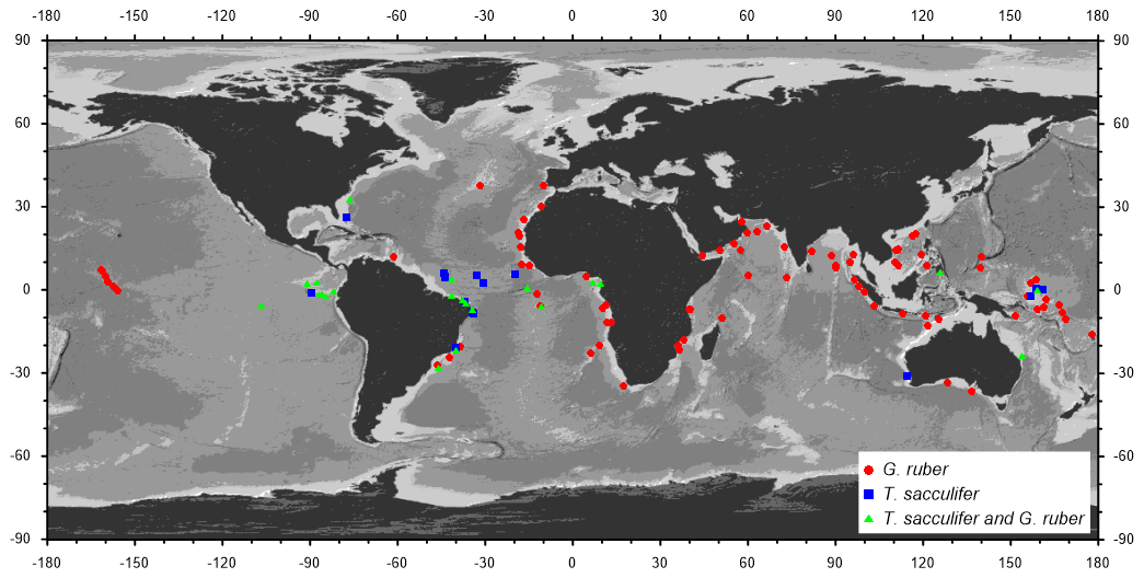
Figure 1 Location of the 127 sediment cores from which data have been compiled for this study. Data from the planktic species G. ruber have been included in 87 cores, and in 18 cores data from T. sacculifer have been included, while 22 cores provide mono-specific data from both species.

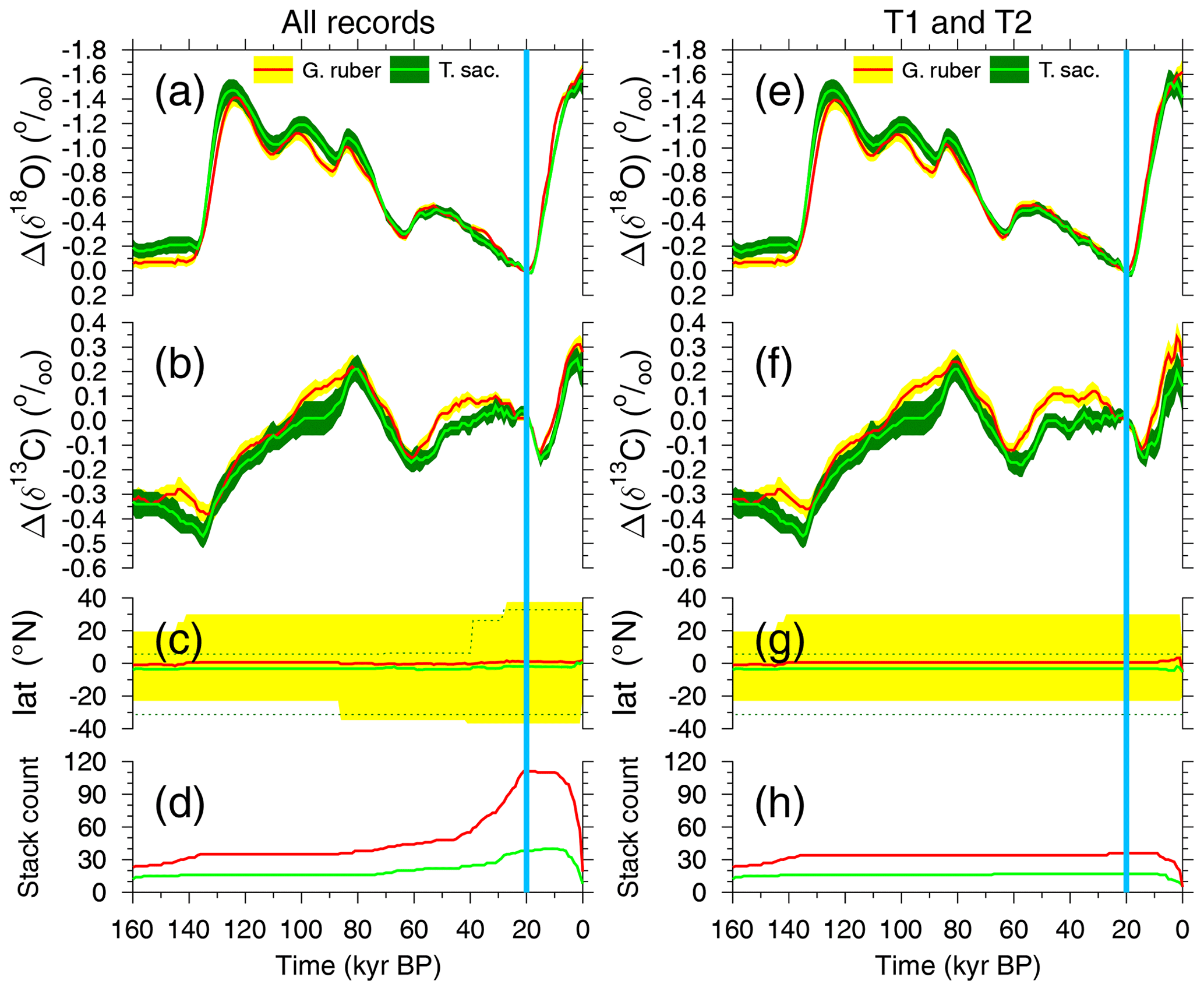
Figure 2 Stacks of anomalies in (a, e) δ¹⁸O and (b, f) δ¹³C from the planktic species G. ruber and T. sacculifer across the last 160 kyr. Mean anomalies (±1 SE) are calculated with respect to the mean of 21–19 kyr BP (vertical blue band). Details of underlying data are found in Table S1. (c, g) Latitudinal distribution of cores contributing to the stack (mean and full range) and (d, h) stack count. Either data from all cores for each species are compiled (a–d) or (e–h) they are compiled from a reduced core selection, in which contributing cores cover both Termination 1 and 2 (T1 + T2).

2.1.2 Stacking of down-core isotope records

Although the size class used for stable isotope measurements can vary considerably among records, it is common practice to use a fairly constant shell size down-core to minimise size-related effects on both oxygen and carbon isotope ratios (e.g. Oppo and Fairbanks, 1989). To provide a common baseline, we corrected all isotope records by their individual mean values for the period from 21 to 19 kyr BP marked as Last Glacial Maximum (LGM) in various plots. To produce final isotope stacks, we averaged all corrected time series and calculated the standard error (SE) of the means at 1 kyr intervals. The final mono-specific stacks of both δ¹⁸O and δ¹³C anomalies based on G. ruber and T. sacculifer are plotted in Fig. 2a, b. The oxygen isotope stacks are also shown here to give a clear reference for G-IG changes: δ¹⁸O has its maxima during peak glacial times and its minima during peak interglacials. In Sect. 3.4 we will come back to these data to discuss the CIE in δ¹⁸O_rub and δ¹⁸O_sac. To test the extent to which the data distribution affects the stacks, we generated two versions of the stacks: one based on all records (Fig. 2a–d) and an alternative based only on records which contain both Terminations (T1 + T2; Fig. 2e–h). The stack counts (Fig. 2d, h) show that the two versions differ mainly in the younger half and that they are identical beyond 85 kyr BP. The latitudinal ranges in the younger half are slightly smaller for the compilations T1 + T2 than when all cores are compiled, but the mean latitudes of all cores are throughout the covered time window of the last 160 kyr in all cases (for both species and for both compilations) close to the Equator (Fig. 2d, g). This consistency in the mean latitude suggests that the incoming light which varied in its annual mean values between ∼ 420 W m⁻² at the Equator and ∼ 330 W m⁻² around latitudes of 40° (Laskar et al., 2004) should only marginally affect the isotopic fractionation (e.g. Spero et al., 1991).

2.2 Benthic δ¹³C

The focus of this study is the δ¹³C of the surface ocean. However, for a rough comparison of δ¹³C changes in the deep ocean, we rely on the published δ¹³C stack constructed from six deep Pacific cores as contained in Lisiecki (2014). The six cores are all ODP cores (677, 846, 849, 1123, 1143 and 1208) from between 2700 and 3500 m water depth, located between 42° S and 36° N. The deep Pacific δ¹³C stack should cover the most-depleted end member of the marine δ¹³C cycle (Fig. 3d) and should give some indication how δ¹³C in the deep ocean is performing in our simulations. More details on the stack are found in Lisiecki (2014).

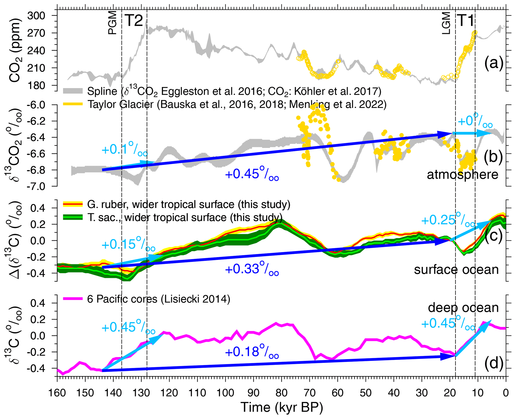
Figure 3 Carbon cycle time series of the last 160 kyr, including the Penultimate Glacial Maximum (PGM) and the Last Glacial Maximum (LGM) and Terminations 1 and 2 (T1 and T2). Spline of atmospheric CO₂ (a) and δ¹³CO₂ (b) based on data from various ice cores (grey, ±1σ around the mean; Köhler et al., 2017a; Eggleston et al., 2016a) and highly resolved recent data from the “horizontal ice core” approach in Taylor Glacier (yellow; Bauska et al., 2016, 2018; Menking et al., 2022b). (c) Δ(δ¹³C_rub) and Δ(δ¹³C_sac) averaging signals in the wider tropical surface ocean (this study, largely based on Mulitza et al., 2022). (d) Deep-ocean δ¹³C from benthic foraminifera stacked from six Pacific cores (Lisiecki, 2014).

2.3 The carbon cycle model BICYCLE-SE

2.3.1 Brief model description

At the core of BICYCLE – the Box model of the Isotopic Carbon cYCLE – sits an ocean (O) with 10 boxes and a terrestrial biosphere consisting of 7 boxes (B) together with a 1-box atmosphere (A), in which the concentration of carbon (as DIC in the ocean, as pCO₂ in the atmosphere and as organic carbon in the biosphere) and both of the isotopes δ¹³C and Δ¹⁴C are traced (Köhler et al., 2005). Furthermore, in the ocean alkalinity, PO${}_{\mathrm{4}}^{\mathrm{3}-}$ as a macro-nutrient and O₂ are represented. From the two variables in the marine carbonate system (DIC and alkalinity), all other variables (CO₂, HCO${}_{\mathrm{3}}^{-}$, CO${}_{\mathrm{3}}^{\mathrm{2}-}$ and pH) are calculated according to Zeebe and Wolf-Gladrow (2001) with updates of the dissociation constants pK₁ and pK₂ (Mojica Prieto and Millero, 2002). The 10 ocean boxes distinguish 100 m deep equatorial (or wider tropical) surface waters in the Atlantic and Indo-Pacific from 1000 m deep surface-ocean boxes in the high latitudes (North Atlantic, Southern Ocean and North Pacific). In the model, wider tropical boxes range from 40° S to 40° N in the Indo-Pacific and to 50° N in the Atlantic, rather similar to the latitudinal coverage of the sediment cores from which Δ(δ¹³C_rub) and Δ(δ¹³C_sac) have been constructed. Deep-ocean boxes represent all waters below 1 km in the three basins: Atlantic, Southern Ocean and Indo-Pacific. In the equatorial regions the waters between 100 and 1000 m depth are described by intermediate boxes. The terrestrial biosphere (Köhler and Fischer, 2004) distinguishes C₃ and C₄ photosynthesis of grasses and trees and soil carbon with different turnover times of up to 1000 years.

The model extension towards the version BICYCLE-SE used here, which can take care of solid Earth processes, is sketched in Fig. 4. The main improvement documented in detail in Köhler and Munhoven (2020) is the implementation of a sediment module, which captures early diagenesis in an 8 cm deep sedimentary mixed layer (M), under which numerous historical layers are implemented. In effect, we now simulate the subsystem of the global carbon cycle consisting of atmosphere, ocean, terrestrial biosphere and sedimentary mixed layer (AOBM) within BICYCLE-SE. In each of the three ocean basins (Atlantic, Southern Ocean and Indo-Pacific) the pressure-dependent carbonate system is calculated for every 100 m water depth, and, depending on the over- or undersaturation of the carbonate ion concentration, CaCO₃ is either accumulated or dissolved. The parametrisation and realisation of the sedimentary processes directly follow Munhoven and François (1996) and Munhoven (1997). The carbon isotopes in the sedimentary mixed layer are only followed in aggregated boxes (one for each of the three ocean basins).

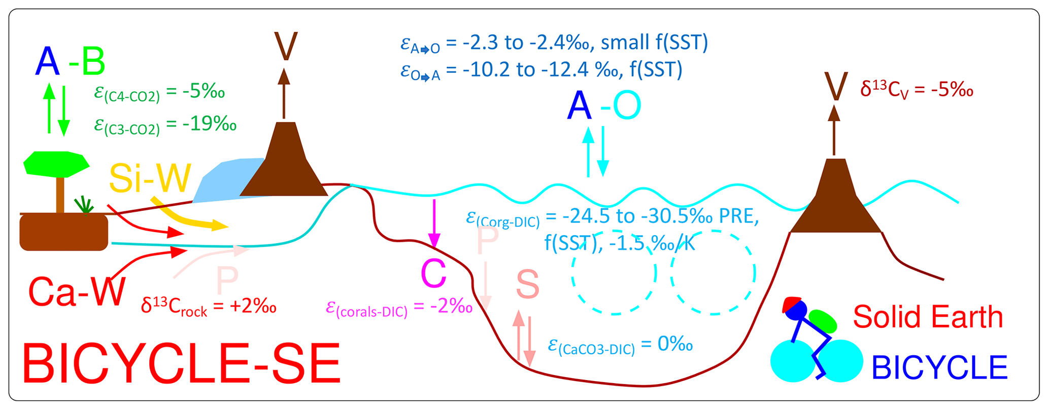
Figure 4 Sketch of the Box model of the isotopic carbon cycle, version solid Earth (BICYCLE-SE), modified from Köhler and Munhoven (2020). V is the outgassing of CO₂ from volcanoes on land potentially and temporally overlain by land ice and from hot-spot island volcanoes (and mid-ocean ridges, not shown) influenced by the changing sea level. C is shallow-water carbonate deposition due to coral reef growth. Si-W is silicate weathering, and Ca-W is carbonate weathering, with different sources of C but both delivering HCO${}_{\mathrm{3}}^{-}$-ions into the ocean. P is the PO${}_{\mathrm{4}}^{\mathrm{3}-}$ riverine input and sedimentary burial, and S is the CaCO₃ sedimentation and dissolution. A–B is the atmosphere–biosphere exchange of CO₂, and A–O is the atmosphere–ocean exchange of CO₂. The cyan-coloured broken circles mimic the two overturning cells in the Atlantic and Indo-Pacific oceans. The isotopic fractionation ε during exchange processes, or the prescribed δ¹³C of external fluxes, is given, summarising the parametrisation of the ¹³C cycle within the model.

Equipping BICYCLE with a process-based sediment module enables the revised model version, BICYCLE-SE, to address questions related to changes in solid Earth carbon fluxes in detail and in the long term. Roughly speaking, the following processes are considered. CO₂ outgassing from volcanoes on land, hot-spot island volcanoes and mid-ocean ridge (MOR) hydrothermal activity is realised as partly being dependent on the changing sea level. Coral reef growth is a known shallow-water carbonate sink, which to some extent also follows sea level rise. The weathering of silicate or carbonate rocks on land consumes different amounts of atmospheric CO₂, with both leading to bicarbonate fluxes into the ocean. These solid Earth processes are not directly coupled with each other. Their implementation in the model might therefore lead to temporal offsets in various variables, to which the sediment module might react in a carbonate compensation feedback. Further details on the model and the time-dependent forcing are found in Köhler and Munhoven (2020). Part of this brief model description has been taken from Köhler (2020).

2.3.2 Complete formulation of the ¹³C cycle in BICYCLE-SE

The following isotopic fractionations are now considered in the BICYCLE-SE model. For this study the whole δ¹³C cycle has been revised. While isotopic fractionations are given here in the ε_(A−B)-notation (in ‰) they are implemented after Zeebe and Wolf-Gladrow (2001) in the model as fractionation factors α_(A−B). Both are related following

$$\begin{array}{}\text{(1)}& {\mathit{\epsilon }}_{(\mathrm{A}-\mathrm{B})}=\mathrm{1000}\cdot ({\mathit{\alpha }}_{(\mathrm{A}-\mathrm{B})}-\mathrm{1}).\end{array}$$

Furthermore, α_(A−B) is related to δ¹³C in reservoirs A and B:

$$\begin{array}{}\text{(2)}& {\mathit{\alpha }}_{(\mathrm{A}-\mathrm{B})}={\displaystyle \frac{{\mathit{\delta }}^{\mathrm{13}}{\mathrm{C}}_{\mathrm{A}}+\mathrm{1000}}{{\mathit{\delta }}^{\mathrm{13}}{\mathrm{C}}_{\mathrm{B}}+\mathrm{1000}}}.\end{array}$$

There is no convention if the initial or final reservoir is given as A or B here; however, here, A is always the final reservoir and B is the initial reservoir of the fractionation process. In some cases, a specific process instead of two reservoirs is mentioned in the subscript, e.g. ε_(a→o) and ε_(o→a) for the atmosphere–ocean gas exchange, for which not only the two different reservoirs but also the direction of the flux play a role in the size of the isotopic fractionation. In that case, the quantified fractionation implies an isotopic depletion connected with the related process for ε<0 ‰.

Air–sea gas exchange.

Using the measurements from Zhang et al. (1995) we formulate, following in most parts Marchal et al. (1998), for the isotopic fractionation during gas exchange to consist of contributions from equilibrium (α^eq) and kinetic (α^k) fractionation (${\mathit{\alpha }}^{\mathrm{total}}={\mathit{\alpha }}^{\mathrm{eq}}\cdot {\mathit{\alpha }}^{\mathrm{k}}$). For the atmosphere-to-ocean CO₂ flux, a temperature-dependent equilibrium fractionation of ${\mathit{\epsilon }}_{\mathrm{a}\to \mathrm{o}}^{\mathrm{eq}}={\mathit{\epsilon }}_{(\mathrm{aq}-\mathrm{g})}^{\mathrm{eq}}=-\mathrm{1.31}+\mathrm{0.0049}\cdot T_{\mathrm{C}}$ between dissolved (aq) and gaseous (g) CO₂ and a ${\mathit{\epsilon }}_{\mathrm{a}\to \mathrm{o}}^{\mathrm{k}}=-\mathrm{1.08}$ ‰ is used. Note that ${\mathit{\epsilon }}_{\mathrm{a}\to \mathrm{o}}^{\mathrm{k}}$ differs by −0.2 ‰ from ${\mathit{\epsilon }}_{\mathrm{o}\to \mathrm{a}}^{\mathrm{k}}=-\mathrm{0.88}$ ‰ for the ocean-to-atmosphere flux, a necessary correction already given in Zhang et al. (1995) but to our knowledge only rarely applied. For the reverse ocean-to-atmosphere flux we use the equilibrium fractionation ${\mathit{\alpha }}_{\mathrm{o}\to \mathrm{a}}^{\mathrm{eq}}={\mathit{\alpha }}_{(\mathrm{aq}-\mathrm{DIC})}^{\mathrm{eq}}={\sum }_i{f}_i{\mathit{\alpha }}_{(\mathrm{aq}-\mathrm{i})}$, with f_i being the relative shares of CO₂, HCO${}_{\mathrm{3}}^{-}$ and CO${}_{\mathrm{3}}^{\mathrm{2}-}$ in DIC in the representative ocean box. Furthermore, from the available measurements in Zhang et al. (1995), we derive ${\mathit{\alpha }}_{(\mathrm{aq}-{\mathrm{HCO}}_{\mathrm{3}}^{-})}=\frac{{\mathit{\alpha }}_{(\mathrm{aq}-\mathrm{g})}}{{\mathit{\alpha }}_{({{\mathrm{HCO}}_{\mathrm{3}}}^{-}-\mathrm{g})}}$, ${\mathit{\alpha }}_{(\mathrm{aq}-{\mathrm{CO}}_{\mathrm{3}}^{\mathrm{2}-})}=\frac{{\mathit{\alpha }}_{(\mathrm{aq}-\mathrm{g})}}{{\mathit{\alpha }}_{({\mathrm{CO}}_{\mathrm{3}}^{\mathrm{2}-}-\mathrm{g})}}$ and ${\mathit{\alpha }}_{(\mathrm{aq}-{\mathrm{CO}}_{\mathrm{2}})}=\mathrm{1}$ using ${\mathit{\epsilon }}_{({\mathrm{CO}}_{\mathrm{3}}^{\mathrm{2}-}-\mathrm{g})}=\mathrm{7.22}-\mathrm{0.052}\cdot T_{\mathrm{C}}$ and ${\mathit{\epsilon }}_{({\mathrm{HCO}}_{\mathrm{3}}^{-}-\mathrm{g})}=\mathrm{10.78}-\mathrm{0.114}\cdot T_{\mathrm{C}}$, with T_C being the sea surface temperature in °C.

Marine biology.

The preindustrial marine export production of organic carbon at 100 m water depth is set to 10 PgC yr⁻¹ (which in the model can increase in glacial periods due to iron fertilisation in the Southern Ocean up to 13 PgC yr⁻¹; Fig. S1d) with a fixed molar rain ratio of organic C:CaCO₃ of 10:1. Existing data on fractionation during marine organic matter production (marine photosynthesis) are rather weak in determining if and how it depends on CO₂ (Young et al., 2013; Brandenburg et al., 2022; Liu et al., 2022). Furthermore, as discussed in Brandenburg et al. (2022), some species might contain so-called carbon concentrating mechanisms and use not CO₂ but HCO${}_{\mathrm{3}}^{-}$ as the source of their carbon, in which case a completely different isotopic fractionation during marine photosynthesis (${\mathit{\epsilon }}_{({\mathrm{C}}_{\mathrm{org}}-\mathrm{DIC})}$) would follow. We base our initial formulation of ${\mathit{\epsilon }}_{({\mathrm{C}}_{\mathrm{org}}-\mathrm{DIC})}$ on the data compilation of δ¹³C_POC in Verwega et al. (2021), who found a dependency on latitude. Using average preindustrial δ¹³C_DIC of +2.5 ‰ (Schmittner et al., 2013) as a starting value and the δ¹³C_POC in Verwega et al. (2021) of −22 ‰, −24 ‰ and −28 ‰ for low, high northern and high southern latitudes, respectively, and approximating ${\mathit{\epsilon }}_{({\mathrm{C}}_{\mathrm{org}}-\mathrm{DIC})}\approx {\mathit{\delta }}^{\mathrm{13}}{\mathrm{C}}_{\mathrm{POC}}-{\mathit{\delta }}^{\mathrm{13}}{\mathrm{C}}_{\mathrm{DIC}}$, we come up with the following isotopic fractionation ${\mathit{\epsilon }}_{({\mathrm{C}}_{\mathrm{org}}-\mathrm{DIC})}$ of −24.5 ‰, −26.5 ‰ and −30.5 ‰ accordingly. This approximation is motivated by the high uncertainties in δ¹³C_POC as documented in Verwega et al. (2021).

The spread in δ¹³C_POC in the data of Verwega et al. (2021) is huge, ranging from −15 ‰ to −35 ‰. Furthermore, they confirmed the finding of earlier studies (Young et al., 2013; Lorrain et al., 2020) that δ¹³C_POC becomes much more depleted over time than what is explainable by the ¹³C Suess effect (Keeling, 1979). Between 1960 and 2010 δ¹³C_POC decreased by about 3±4‰. The Suess effect shows a decrease in atmospheric δ¹³CO₂ of about 1.5 ‰ during that time (Rubino et al., 2013), and it is known that in the ocean the Suess effect is decreasing with depth (Eide et al., 2017). At the same time, the global mean temperature rose by about 0.8 K (Rohde and Hausfather, 2020). This shift in δ¹³C_POC is probably caused by a shift in the composition of the phytoplankton communities. We therefore use the values derived in the previous paragraph from Verwega et al. (2021) as our preindustrial parameter values of ${\mathit{\epsilon }}_{({\mathrm{C}}_{\mathrm{org}}-\mathrm{DIC})}$, to which we add a temperature-dependent part of −1.5 ‰ for any K the sea surface temperature in the relevant surface-ocean box disagrees with from its preindustrial value. The assumed value fits in the range of recent temperature-dependent δ¹³C_POC found in Verwega et al. (2021) and has been obtained by tuning to simulate δ¹³CO₂ at preindustrial times to be similar to its values at the LGM, as seen in the ice core data (Fig. 3b). This leads to ${\mathit{\epsilon }}_{({\mathrm{C}}_{\mathrm{org}}-\mathrm{DIC})}$ at the LGM of −19.3 ‰, −20.4 ‰ and −24.4 ‰ for low, high northern or high southern latitudes, respectively.

Data are also rather uncertain for the isotopic fractionation during the formation of CaCO₃. We assume, in agreement with Buitenhuis et al. (2019), that 65 % of the CaCO₃ exported in the abyss consists of aragonite and 35 % of calcite. Calcite is either produced by coccolithophores or planktic foraminifera. Some coccolithophore species suggest an enrichment, while others suggest a depletion in δ¹³C in their shells with respect to δ¹³C_DIC in the surrounding water (Ziveri et al., 2003). For planktic foraminifera, the CIE is one of various possible processes of isotopic fractionation hypothesised to occur during hard-shell formation (Bijma et al., 1999; Zeebe et al., 2008; Kimoto, 2015). Isotopic fractionation factors are in comparison to ${\mathit{\epsilon }}_{({\mathrm{C}}_{\mathrm{org}}-\mathrm{DIC})}$ rather small and, in the case of the CIE, species-specific (Spero et al., 1999). We therefore choose in the model to set the fractionation during calcite production to be neutral with respect to ¹³C, thus ${\mathit{\epsilon }}_{(\mathrm{cal}-\mathrm{DIC})}=\mathrm{0}$ ‰, but we will consider the CIE in post-processing when comparing simulations with reconstructions. For simplicity and due to missing further evidence for fractionation during aragonite production, ε_(ara−DIC) was also kept at 0 ‰. More generally, we keep ${\mathit{\epsilon }}_{({\mathrm{CaCO}}_{\mathrm{3}}-\mathrm{DIC})}=\mathrm{0}$ ‰.

The shallow-water sink of carbonate in corals is assumed to have a δ¹³C that follows after an isotopic fraction of ${\mathit{\epsilon }}_{(\mathrm{corals}-\mathrm{DIC})}=-\mathrm{2}$ ‰ from the δ¹³C of the DIC in the surface waters. This value is based on a combination of recent data, paleo-data from the Great Barrier Reef and insights from simulations (Linsley et al., 2019; Felis et al., 2022).

Terrestrial biosphere.

On land, isotopic fractionation is only assumed to occur during photosynthesis, with ${\mathit{\epsilon }}_{({\mathrm{C}}_{\mathrm{3}}-{\mathrm{CO}}_{\mathrm{2}})}=-\mathrm{19}$ ‰ and ${\mathit{\epsilon }}_{({\mathrm{C}}_{\mathrm{4}}-{\mathrm{CO}}_{\mathrm{2}})}=-\mathrm{5}$ ‰ for C₃ (all woody plants and some grasses) and C₄ (some other grasses) photosynthesis, respectively (Vogel, 1993; Lloyd and Farquhar, 1994).

External fluxes to the AOBM subsystem.

The volcanic CO₂ outgassing flux is assumed to have a fixed δ¹³C signature (δ¹³C_V) of −5.0 ‰, the typical mean value for volcanic outgassing (e.g. Deines, 2002; Roth and Joos, 2012), but note that the uncertainty is ±3 ‰.

From the two weathering fluxes based on either silicate or carbonate rocks, only the latter has a contribution which brings new carbon into the system. Here, 50 % of the carbon that is entering the ocean as bicarbonate (the weathering product) has a δ¹³C signature (δ¹³C_rock) of +2 ‰, which is identical to the most likely δ¹³C values in carbonate rocks formed during the Phanerozoic (Bachan et al., 2017). The carbon for the other half of the carbonate weathering flux and for all of the silicate weathering flux is assumed to come from CO₂ in the soil environment. We therefore assume that this CO₂ is dominated by soil respiration fluxes; therefore, a δ¹³C signature that corresponds to the mean value of the two soil carbon boxes is assumed here.

To balance the inflow of ¹³C via volcanism and weathering, the model has been tuned for long-term stable mean δ¹³C values in the AOBM subsystem by the following sink: about 6 % of the organic carbon that is exported from the surface boxes into the abyss is assumed to be lost in the sediment. Note that this number has been tuned with the previous version of the ¹³C cycle in operation (Köhler and Munhoven, 2020), but it has not been revised thereafter.

2.3.3 Simulation setup and scenarios

The BICYCLE-SE model simulates the global carbon cycle as a function of changing time-dependent physical boundary conditions (forcing), which are nearly identical to the simulations published in Köhler and Munhoven (2020) and which are also described in that study in detail. Briefly, ocean circulation is prescribed from modern data of the WOCE experiment, while its main temporal changes are restricted to (a) the AMOC, which is reduced from modern/interglacial 16 to 10 Sv during glacial periods (Fig. S1b), and (b) Southern Ocean (SO) vertical deep mixing, which is a function of SO sea surface temperature (Fig. S1c). Ocean and land temperatures are prescribed from reconstructions (Fig. S1e), and ocean salinity is varied as a function of the prescribed sea level (Fig. S1a). Additionally, aeolian iron input in the SO is assumed to follow dust fluxes measured in Antarctic ice cores, which might change marine biology in the SO from an iron-limited to an iron-unlimited regime, increasing glacial export production of organic matter to the deep ocean (Fig. S1d). The standard scenario used here, SEi, is, apart from the revised δ¹³C cycle, nearly identical to the scenario SE in Köhler and Munhoven (2020). The only difference here is that in the application we revised the applied equatorial sea surface temperature (SST). It has been based in previous applications on changes in planktic δ¹⁸O in only one ODP record. Now we use the SST stack from Barth et al. (2018), which is based on a compilation of SSTs from 15 non-polar sediment cores. This leads to only minor changes in atmospheric CO₂ of less than 5 ppm, but it is important for the ¹³C cycle and its temperature dependencies (isotopic fractionation during atmosphere–ocean gas exchange and during carbon uptake by the marine biology). Simulations are started from interglacial conditions around 210 kyr BP. Scenario SEi0 is only performed to illustrate how the implementation of the temperature dependency in ${\mathit{\epsilon }}_{({\mathrm{C}}_{\mathrm{org}}-\mathrm{DIC})}$ improves the simulated ¹³C cycle, illustrated by plotting atmospheric δ¹³CO₂ against data in Fig. 5b.

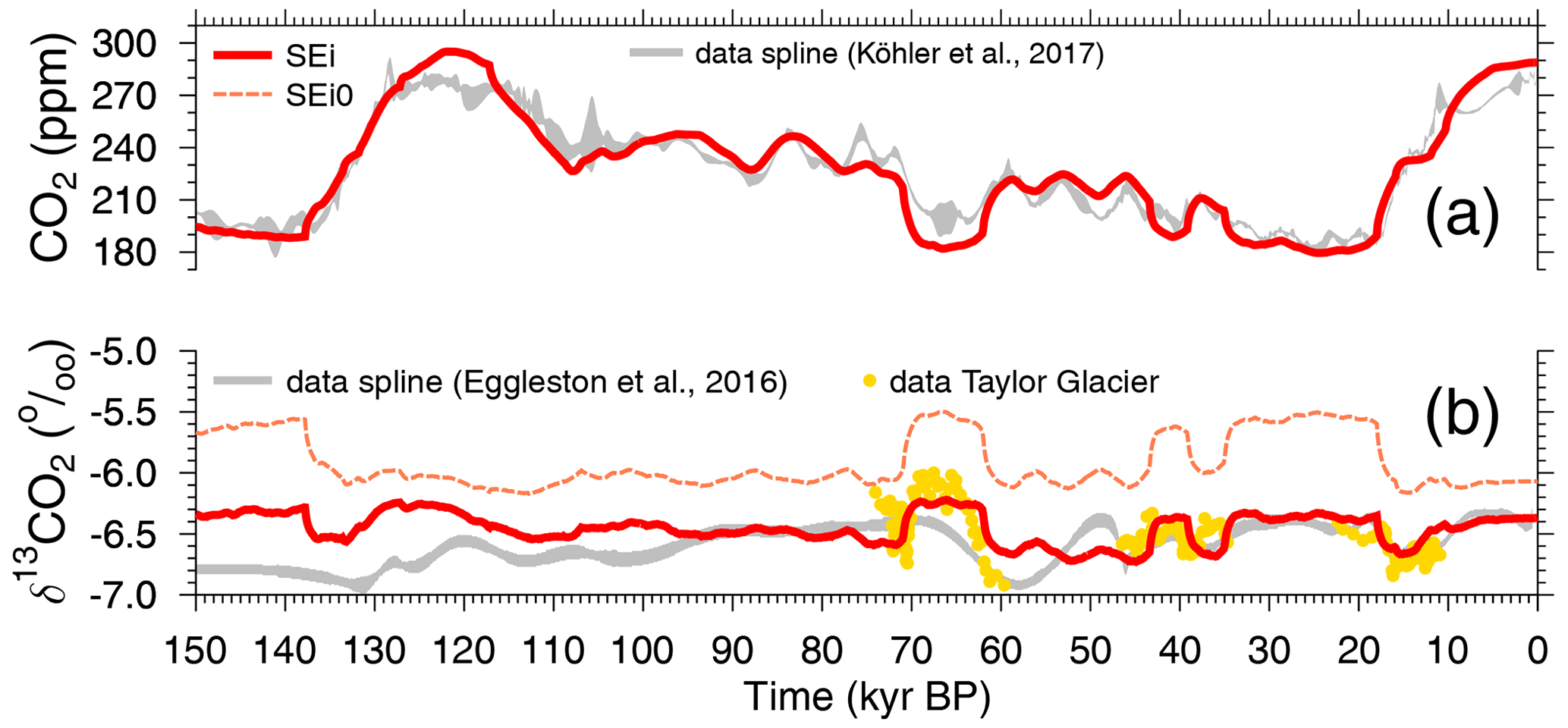
Figure 5 Simulation results and comparison to data splines for (a) atmospheric CO₂ and (b) atmospheric δ¹³CO₂. Results for scenario SEi (standard) and SEi0 are shown. The latter differs from the standard run by a lack of temperature dependency in ${\mathit{\epsilon }}_{({\mathrm{C}}_{\mathrm{org}}-\mathrm{DIC})}$.

Simulated changes in the atmospheric record are already not too far away from the reconstructions in scenario SEi, especially in CO₂ (Fig. 5a). However, to bring the carbon cycle in the atmosphere and the surface ocean as close to the reconstructions as possible, we perform additional simulations in which the atmospheric δ¹³CO₂ alone (scenario C1) or together with atmospheric CO₂ (scenario C1CO2) is forced by the reconstructions. Here, we use the data splines as plotted in Fig. 3a, b (Eggleston et al., 2016a; Köhler et al., 2017a) and ignore the higher resolved data from Taylor Glacier, since these more abrupt changes in δ¹³CO₂ are either covered to a large extent during the last 50 kyr in the dynamics of the spline (Bauska et al., 2016, 2018) or are probably not recorded in our marine sediment records around 70 kyr BP (Menking et al., 2022b). This implies that internally calculated fluxes are overwritten by changes that are necessary to keep the simulated atmospheric carbon variables identical to the reconstructions. This approach is typically applied in CO₂-concentration-driven present-day or future ocean carbon cycle simulations (e.g. Hauck et al., 2020). It has already been used in BICYCLE-SE for ¹⁴C to obtain radiocarbon in the surface ocean as close to the data as possible during the construction of the most recent marine radiocarbon calibration curve Marine20 (Heaton et al., 2020b) and subsequent studies (Köhler et al., 2022). However, since atmospheric CO₂ and δ¹³CO₂ are normally prognostic variables of the model and their calculated changes should be derived from the model's differential equations followed by a proper integration scheme, this approach slightly violates the mass conservation. It nevertheless guarantees that simulated surface-ocean variables of the carbon cycle within the model realm are as consistent as possible with the atmospheric reconstructions. An overview of the applied simulation scenarios is compiled in Table 1.

(Eggleston et al., 2016a)(Eggleston et al., 2016a; Köhler et al., 2017a)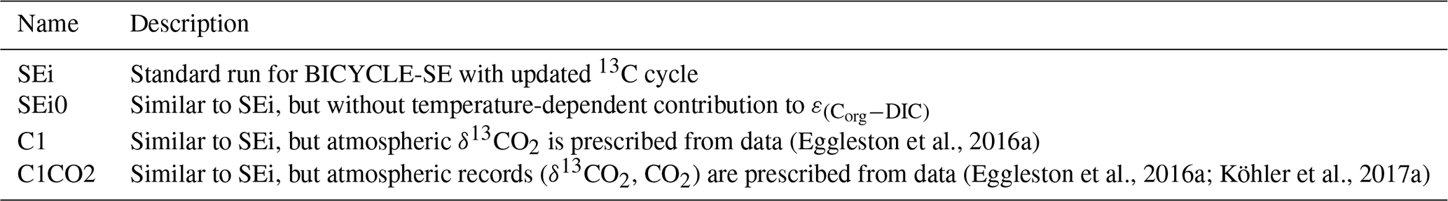

Table 1 Overview of simulation scenarios.

2.4 Data analysis

Linear regression was performed with the software MATLAB (The MathWorks Inc., 2023). The uncertainties of the fits are approximated by root-mean-square errors calculated after $s=\sqrt{\frac{\mathrm{1}}{n}{\sum }_{i=\mathrm{1}}^n(y_i-f_i{)}^{\mathrm{2}}}$, with f_i being the calculated values according to the linear regression equations. In cases in which the uncertainties in both variables should be considered, we used the function “linfitxy”, version 1.2.0.0 (Browaeys, 2023). The frequency analysis was performed using R (R Core Team, 2023), including the function “coh” from the R package seewave, version 2.2.3, calculating coherence.

3 Results and discussion

3.1 Overview on ¹³C cycle changes over the last 160 kyr

Reconstructed changes in the late Quaternary carbon cycle are still not completely understood. The ice cores give us a precise picture of atmospheric CO₂ (Bereiter et al., 2015; Köhler et al., 2017a) (Fig. 3a), which in the meantime has also been met reasonably well with various different carbon cycle models (e.g. Menviel et al., 2012; Ganopolski and Brovkin, 2017; Khatiwala et al., 2019; Köhler and Munhoven, 2020). These findings suggest that the main processes responsible for the observed changes on orbital timescales might indeed have been identified, although results are to some extent model-dependent and improvements in details are certainly necessary.

The corresponding atmospheric δ¹³CO₂, now available over the last 155 kyr (Eggleston et al., 2016a), is, however, still waiting for a process-based interpretation of all its features (Fig. 3b). Since δ¹³CO₂ helps to pinpoint processes responsible for CO₂ changes, any simulation that is able to explain one without the other might need to be interpreted with caution. Models suggest that especially physical and biological processes in the Southern Ocean processes robustly influence δ¹³CO₂, while the impact of the Atlantic meridional overturning circulation (AMOC) on δ¹³CO₂ seems to be model-dependent (Menviel et al., 2015). Consequently, the abrupt drop in δ¹³CO₂ at the onset of Termination 1 (T1) (Smith et al., 1999; Schmitt et al., 2012) is nowadays understood to be caused by marine processes, while subsequent δ¹³CO₂ changes during T1 and its recovery during the Holocene to LGM-like values were potentially related to a mixture of oceanic and terrestrial processes (Köhler et al., 2005; Bauska et al., 2016).

Two largely unexplained features stand out in the 155 kyr δ¹³CO₂ record. Firstly, there is a long-term trend of +0.45 ‰ from the Penultimate Glacial Maximum (PGM) and the Last Glacial Maximum (LGM). When first discovered (Schneider et al., 2013), it was hypothesised that changes in the isotopic composition of solid Earth fluxes or of their intensities or long-term peat build-up might be responsible for them. Secondly, a 0.5 ‰ deep and nearly 20 kyr long minimum centred around 58 kyr BP happened, rather uncorrelated with CO₂ changes. Eggleston et al. (2016a) hypothesise that the δ¹³CO₂ minimum might have been partially caused by a change in ocean stratification between Marine Isotope Stage (MIS) 4 and MIS 3, allowing a different amount of isotopically light carbon to be stored in the deep ocean. Recently, high-resolution data of δ¹³CO₂ from Taylor Glacier covering 74 to 59.5 kyr BP, including MIS 4 and the drop into the δ¹³CO₂ minimum, have been published (Menking et al., 2022b), showing more variability and, between 66 and 60 kyr BP with −1 ‰, a change twice as large as that previously contained in the smoothed record of Eggleston et al. (2016a). Menking et al. (2022b) also first performed model simulations in order to understand which processes might be responsible for the reconstructed changes in the carbon cycle. However, to our knowledge, none of the ideas put forward in Schneider et al. (2013) for the long-term trend in δ¹³CO₂ have so far been convincingly and successfully verified with carbon cycle model simulation. Furthermore, 400–500 kyr variability in δ¹³C related to slow eccentricity changes found throughout the Cenozoic (e.g. Pälike et al., 2006; Russon et al., 2010; Ma et al., 2011; Wang et al., 2014; Paillard, 2017) might be superimposed on faster variations, making a process-based understanding of observed changes in δ¹³CO₂ even more challenging.

Sediment cores covering the Anthropocene clearly show that the δ¹³C of G. ruber and T. sacculifer shells (δ¹³C_rub and δ¹³C_sac) faithfully reflects changes in δ¹³C_DIC caused by the δ¹³C Suess effect (Al-Rousan et al., 2004; Black et al., 2011), albeit with a notable offset. This offset might be influenced by the CIE (e.g. Spero et al., 1997), light intensity (e.g. Spero et al., 1991) and the size of the foraminiferal shells (e.g. Oppo and Fairbanks, 1989). Our new mono-specific stacks from the wider tropical surface ocean of Δ(δ¹³C_rub) and Δ(δ¹³C_sac) (Fig. 3c) contain a G-IG rise of 0.25 ‰ across T1 but of only 0.15 ‰ across T2, while atmospheric δ¹³CO₂ at the same time rose by 0.1 ‰ (T2) or stayed constant (T1) (Fig. 3b), showing local minima during terminations in both records. Deep-ocean benthic δ¹³C (Fig. 3d) is approximated here by a stack from six deep Pacific cores (Lisiecki, 2014), which contains a G-IG rise of 0.45 ‰ across both T1 and T2. This value is on the upper end of the 95 % confidence interval of compilations of marine δ¹³C changes across T1 (Peterson et al., 2014; Peterson and Lisiecki, 2018), which suggests a representation of global ocean-wide changes. The marine time series, both from the surface ocean and the deep ocean, also contain wide and deep minima around 60 kyr BP, similarly to the smoothed atmospheric δ¹³CO₂ data of Eggleston et al. (2016a) but differently to the more highly resolved Taylor Glacier δ¹³CO₂ of Menking et al. (2022b). Furthermore, all marine δ¹³C data, similarly to the atmospheric δ¹³CO₂, contain a long-term rise from the PGM to the LGM (about +0.33 ‰ in the wider tropical surface ocean and +0.18 ‰ in the deep Pacific; Fig.3), which might be potentially connected to the 400–500 kyr variability.

Figure 6 Scatter plot of our new stacks, (a) Δ(δ¹³C_rub) versus Δ(δ¹³C_sac) and (b) Δ(δ¹⁸O_rub) versus Δ(δ¹⁸O_sac). Data stacks without corrections for the CIE are plotted. The time series are restricted to data from the last 150 kyr to allow a comparison later on with simulation results, which were based on the only 155 kyr long atmospheric δ¹³CO₂ record. Linear regressions using only the mean values and also when using uncertainties in both x and y are performed. The root-mean-square error is depicted by s.

Before we start with a deeper model-based interpretation of the ¹³C cycle, we have a closer look at our new isotope stacks. The size of the CIE as detected from laboratory experiments in both species differs by a factor of nearly 2: a change of −0.0089 ‰ and −0.0047 ‰ in δ¹³C per µmol kg⁻¹ of [CO${}_{\mathrm{3}}^{\mathrm{2}-}$] for G. ruber and T. sacculifer, respectively, and a change of −0.0022 ‰ and −0.0014 ‰ in δ¹⁸O per µmol kg⁻¹ of [CO${}_{\mathrm{3}}^{\mathrm{2}-}$] for G. ruber and T. sacculifer, respectively (Spero et al., 1999). Therefore, if the CIE plays a role in how the isotopes of the surface ocean are recorded in the foraminifera shells on orbital timescales, then the two mono-specific time series in both δ¹³C and δ¹⁸O should differ. At first glance (Fig. 2a, b) the time series are remarkable similar. A more quantitative evaluation is obtained by calculating the linear regression from scatter plots when results based on one species are plotted against those of the other. Doing so (Fig. 6) reveals for δ¹³C that, on average, changes are identically recorded in both species. In other words, the linear slope of Δ(δ¹³C_rub) against Δ(δ¹³C_sac) is 0.98 $(r^{\mathrm{2}}=\mathrm{0.95},s=\mathrm{0.04}\mathrm{‰})$, or 0.99±0.03 (r²=0.95) when considering the uncertainties of our stack during regression. For δ¹⁸O the agreement is only slightly worse: the regression slope of δ¹⁸O_rub against δ¹⁸O_sac is 0.96 $(r^{\mathrm{2}}=\mathrm{0.96},s=\mathrm{0.09}\mathrm{‰})$, or 0.98±0.01 (r²=0.96) with uncertainties. Since Δ(δ¹³C_rub) and Δ(δ¹³C_sac) are on average recording virtually the same changes, it is difficult to image how the species-specific CIE can play a role here. Due to the small amplitudes of the CIE in δ¹⁸O, it is as yet inconclusive if the CIE plays a role for Δ(δ¹⁸O_rub) versus Δ(δ¹⁸O_sac).

3.2 Simulated δ¹³C cycle using the BICYCLE-SE model

General dynamics of the global carbon cycle in the BICYCLE-SE model have been analysed in detail in Köhler and Munhoven (2020). We focus here on the revised δ¹³C cycle but see how atmospheric CO₂ in scenario SEi meets the ice core data in Fig. 5a. Note that some analysis of δ¹³C in the precursor model BICYCLE without solid Earth contributions has been described in Köhler et al. (2010), who showed that the model misses variations in δ¹³C related to periodicities longer than 100 kyr.

Atmospheric δ¹³CO₂ (Eggleston et al., 2016a) is met by the results from scenario SEi only roughly, including some millennial-scale variations around 50–30 kyr BP and the transition from the LGM to preindustrial, showing some deficit in the second half of T1 and in the Holocene (Fig. 5b). The PGM-to-LGM trend of 0.45 ‰ and the minimum around 60 kyr BP are both largely unexplained in this simulation. The attribution of changes in δ¹³CO₂ to individual processes in the ocean and land carbon cycle has been done before for the precursor model BICYCLE (Köhler et al., 2005, 2010) and is not repeated here, since the misfit to the data indicates some fundamental shortcomings.

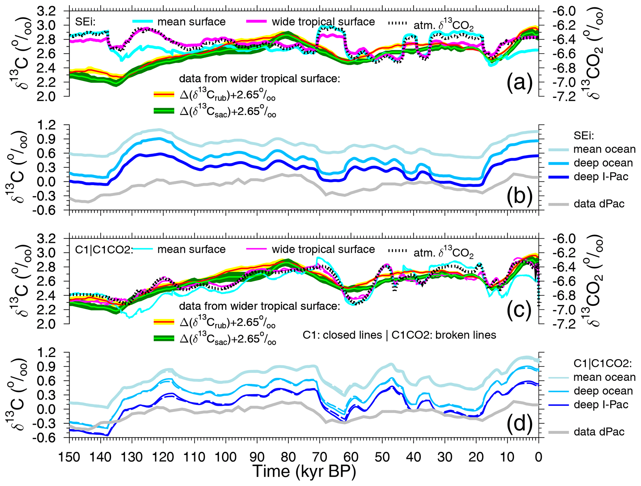
Figure 7 Simulated surface- and deeper-ocean δ¹³C time series from scenario SEi (a, b) and scenarios C1 and C1CO2 (c, d) compared with reconstructions. (a, c) Simulated δ¹³C_DIC in the global mean surface ocean and in the wider tropical surface ocean together with simulated atmospheric δ¹³CO₂ (right y axis) are plotted together with our new stacks from the wider tropical surface ocean, with Δ(δ¹³C_rub) and Δ(δ¹³C_sac) shifted by +2.65 ‰ to meet simulated surface δ¹³C_DIC at the LGM. In panels (b) and (d), simulated δ¹³C_DIC for the deep Indo-Pacific (I-Pac), the mean deep ocean and the mean global ocean are plotted together with δ¹³C from benthic foraminifera stacked from six cores in the deep Pacific (dPac) (Lisiecki, 2014). In panels (c) and (d), the scenarios C1 (closed lines) and C1CO2 (broken lines) are plotted together. Most of the time the differences between both are so small that the lines are indistinguishable.

The way in which simulated changes in atmospheric δ¹³CO₂ compare to simulated changes in various marine δ¹³C_DIC time series is shown for scenario SEi in Fig. 7a, b. Both global mean surface δ¹³C_DIC and wider tropical surface δ¹³C_DIC show clear similarities with atmospheric δ¹³CO₂. Here, surface values are area-weighted averages covering either the global ocean or the two equatorial ocean boxes in the case of the wider tropics, which spatially cover a similar area to the sediment cores used for our new stacks, Δ(δ¹³C_rub) and Δ(δ¹³C_sac). During glacial times and the onset of deglaciations, the dynamics in the global mean surface δ¹³C_DIC (cyan line in Fig. 7a) are in close agreement with δ¹³CO₂ in the atmosphere (broken black line in Fig. 7a), while for the later part of the deglaciations and the interglacials the dynamics in the wider tropical surface δ¹³C_DIC (magenta line in Fig. 7a) fit better to δ¹³CO₂ in the atmosphere. This difference is probably explained by the dynamics in the polar oceans. During glacial times, the Southern Ocean is highly stratified with little vertical exchange between the surface ocean and the deep ocean. This stratification breaks down during the terminations and in the interglacials, allowing a faster exchange of tracers between the surface ocean and the deep ocean, leading to smaller surface-to-deep gradients in δ¹³C_DIC in the polar oceans. In other words, the lower deep-ocean δ¹³C_DIC values have a larger impact on polar surface δ¹³C_DIC during interglacials than during glacials, leading to a divergence in δ¹³C_DIC in the global mean surface and in the wider tropical surface ocean. The scatter plots between atmospheric δ¹³CO₂ and either global mean surface or wider tropical surface-ocean δ¹³C_DIC show that the latter has the higher correlation (Fig. S2; r²=0.82 vs. r²=0.59). Furthermore, frequency analysis showed that the coherence between atmospheric δ¹³CO₂ and wider tropical surface-ocean δ¹³C_DIC is in periodicities slower than 20 kyr higher than between atmospheric δ¹³CO₂ and global mean surface-ocean δ¹³C_DIC (Fig. S3a). This implies that simulations which agree in atmospheric δ¹³CO₂ with reconstructions (which will be achieved later on in scenarios C1 and C1CO2) should contain a very likely realisation of δ¹³C_DIC in the wider tropical surface ocean. A comparison of these simulated time series with our new mono-specific δ¹³C stacks should therefore enable us to address if and how δ¹³C has been modified during hard-shell formation. For scenario SEi the misfit in simulated wider tropical surface-ocean δ¹³C_DIC and the new δ¹³C reconstructions (Fig. 7a) is large, but it is as yet unclear if this discrepancy can be explained by the CIE or by other processes.

To understand how representative the reconstructed δ¹³C stack from benthic foraminifera in six deep Pacific cores (Lisiecki, 2014) might be, we compare it with various different simulated time series: δ¹³C_DIC in the deep Indo-Pacific, in the mean deep ocean and in the mean ocean (Fig. 7b). Here, deep-ocean results from the model refer to ocean boxes that contain waters deeper than 1 km. As expected, the deep Indo-Pacific contains the end member of the δ¹³C cycle with the most depleted values. The mean deep-ocean δ¹³C_DIC is offset by 0.2 ‰–0.4 ‰ towards more positive values and shows larger G-IG amplitudes than δ¹³C_DIC does in the deep Indo-Pacific. The mean ocean is again 0.2 ‰–0.4 ‰ more positive in δ¹³C_DIC than the mean deep ocean, again with smaller G-IG amplitudes of 0.53 ‰ across T1. This number compares δ¹³C_DIC in the last 6 kyr with the mean at the LGM (23–19 kyr BP), similarly as in Peterson et al. (2014), who proposed a mean ocean rise in δ¹³C by 0.34±0.19 ‰. However, be aware that in Peterson et al. (2014) the CIE in benthic foraminifera as deduced in Schmittner et al. (2017) is not included. This suggests that the reconstructions are potentially recording a smaller G-IG change in δ¹³C than how δ¹³C_DIC in the deep ocean might have changed.

When discussing the results of scenario SEi (Fig. 7a), we have shown that, once changes in the atmospheric δ¹³CO₂ are met by the simulations, the model should then also give a reasonable answer for what δ¹³C_DIC in the wider tropical surface ocean might have looked like. Furthermore, the close agreement in simulated and reconstructed atmospheric CO₂ (Fig. 5a) suggests that the assumed carbon cycle changes in our approach might be one possible realisation that is not too far away from the real-world changes. However, the misfit between simulation results from scenario SEi and reconstruction in the δ¹³C cycle, where linear regressions between simulations and reconstructions found no correlation at all (r²≤0.02; Fig. S4a, b), is not easily fixed. To improve our results, we force the model with the atmospheric records (scenario C1 only using δ¹³CO₂ and scenario C1CO2 using both δ¹³CO₂ and CO₂) to have conditions in the surface ocean as close to reconstructions as possible. Doing so leads to even tighter correlations between simulated atmospheric δ¹³CO₂ and simulated δ¹³C_DIC in the surface ocean than what we obtained for scenario SEi: the r² correlations between these variables are in scenarios C1 and C1CO2, with prescribed atmospheric δ¹³CO₂ ≥ 0.77 and ≥ 0.88 for global mean surface δ¹³C_DIC and wider tropical surface δ¹³C_DIC, respectively (Fig. S2). Again, the coherence is higher between atmospheric δ¹³CO₂ and the wider tropical surface-ocean δ¹³C_DIC than between atmospheric δ¹³CO₂ and the global mean surface-ocean δ¹³C_DIC (Fig. S3b). Furthermore, in both scenarios, the changes in simulated δ¹³C_DIC in the wider tropical surface ocean agree remarkably well (r² between 0.76 and 0.78; Fig. S4c–f) with changes in our new stacks Δ(δ¹³C_rub) and Δ(δ¹³C_sac) without consideration of the CIE (Fig. 7c), at least on orbital timescales. This effect is also seen by the rise in coherence between simulated wider tropical surface δ¹³C_DIC and both our stacks from less than 0.1 (scenario SEi) to higher than 0.7 (scenario C1CO2) in the 41 and 100 kyr bands (Fig. S3c, d), while in the precession bands (19 and 23 kyr) the coherence stayed below 0.6. Some more abrupt changes contained in the simulations are not recorded in the reconstructions, probably because bioturbation in the surface sediments, together with the stacking procedure, prevent our marine records from successfully resolving millennial-scale features. Thus, our forcing of atmospheric carbon records with data therefore seems to be a promising approach to obtain simulated surface ocean in agreement with reconstructions for the slow-frequency bands (41 kyr and beyond), while it seems to fail for precession and faster changes. When forcing atmospheric δ¹³CO₂ by data, the temperature-dependent isotopic fractionation during marine photosynthesis in ${\mathit{\epsilon }}_{({\mathrm{C}}_{\mathrm{org}}-\mathrm{DIC})}$ is only of minor importance for the simulated surface-ocean δ¹³C_DIC. If this effect is switched off, the δ¹³C_DIC in the wider tropical surface ocean differs in general by less than 0.05 ‰ from the values in scenario C1.

Furthermore, deep-ocean δ¹³C_DIC is now, on an orbital timescale, also in better agreement with the data (Fig. 7d), the r² of a linear regression between simulated deep Indo-Pacific δ¹³C_DIC, and the reconstructed deep Pacific rises from 0.49 for scenario SEi to 0.77 and above for the scenarios forced by atmospheric carbon records (Fig. S5), although the rise in mean ocean δ¹³C_DIC during T1 has now been increased to 0.59 ‰. Considering a CIE of $-\mathrm{2.6}\times {\mathrm{10}}^{-\mathrm{3}}$ ‰ per µmol kg⁻¹ of [CO${}_{\mathrm{3}}^{\mathrm{2}-}$] disturbance for epibenthic foraminifera (Schmittner et al., 2017), simulated variations in deep-ocean [CO${}_{\mathrm{3}}^{\mathrm{2}-}$] of +20 µmol kg⁻¹ (Köhler and Munhoven, 2020) would translate to a comparably small reduction in deep Pacific benthic δ¹³C of up to 0.05‰. While the timing of changes in deep-ocean [CO${}_{\mathrm{3}}^{\mathrm{2}-}$] with highest values during the deglaciation is crucial to assess how such a benthic CIE would reduce the existing data–model mismatch, a more thorough assessment of the benthic CIE would require the comprehensive compilation of benthic δ¹³C time series in different ocean basins, which is beyond the scope of this study. Note that the approximated amplitude of this benthic CIE is close to the measurement error of benthic δ¹³C.

3.3 The importance of the carbonate ion effect for wider tropical surface-ocean δ¹³C

Although the initial analysis of our results when forced with atmospheric records already suggests only a minor, if any, role for the CIE in the interpretation of stacked mono-specific δ¹³C on orbital timescales, in the following section we make a more quantitative assessment. The CIE has not yet been implemented in the ¹³C cycle of the model, but it is only investigated here in post-processing. The carbonate ion concentration of either global mean surface waters or wider tropical mean surface waters in our simulations is tightly anti-correlated with atmospheric CO₂ (r²≥0.93; Fig. S6), which is a consequence of the marine carbonate system (Zeebe and Wolf-Gladrow, 2001). Both scenarios C1 and C1CO2 lead to rather similar results here, which suggests that the CO₂ forcing in scenario C1CO2 and its violation of mass conservation are perturbing the carbon cycle only slightly. To stay as closely as possible to the reconstructions, we nevertheless continue in the following section by using results from scenario C1CO2, but results differ only slightly when based in scenario C1; thus our conclusions are independent from this choice.

Thus, CO${}_{\mathrm{3}}^{\mathrm{2}-}$ in the wider tropical surface ocean in the simulation typically falls from maximum glacial values of ∼ 320 µmol kg⁻¹ to interglacial minima of ∼ 250 µmol kg⁻¹ across both Terminations 1 and 2 (Fig. 8a). This translates into a potential CIE of about 0.62 ‰ (Fig. 8b) for G. ruber when we use the slope of $m=-\mathrm{0.0089}$ ‰ per µmol kg⁻¹ change in $\left[{\mathrm{CO}}_{\mathrm{3}}^{\mathrm{2}-}\right]$ and of 0.33 ‰ for T. sacculifer (slope of $m=-\mathrm{0.0047}$ ‰ per µmol kg⁻¹ change in $\left[{\mathrm{CO}}_{\mathrm{3}}^{\mathrm{2}-}\right]$) (Spero et al., 1999). The y axis intercepts of the complete regressions for the CIE is determined in order to have a maximum agreement between reconstructions and simulations during the LGM. When comparing the potential CIE to the simulated LGM-to-preindustrial (PRE) amplitude of only 0.16 ‰ in wider tropical surface waters (Fig. 8c), the CIE-to-G-IG ratios are between a factor of 2 and 4, and CIE signals should clearly stand out in the paleo-records. If we add this CIE to our simulated mean equatorial surface-ocean δ¹³C_DIC (Fig. 8c), we end up with time series, which should compare well with the mono-species stacks of Δ(δ¹³C_rub) and Δ(δ¹³C_sac) (Fig. 8d). However, this is not the case. The r² in the linear regressions between CIE-corrected δ¹³C_DIC in wider tropical surface waters and reconstructions is reduced to 0.54 (G. ruber) and 0.68 (T. sacculifer), while it had been ≥ 0.76 without CIE correction (Figs. S4, S7). When plotting results as hypothetically recorded in both species against each other, we obtain a slope of 1.26 (Fig. S8a). The slope between the stacked mono-specific δ¹³C time series without further correction for a CIE was ∼ 0.99 (Fig. 6a). The consideration of the CIE did not lead to time series which agree better with each other. Thus, we conclude that both species, G. ruber and T. sacculifer, are already good recorders of changes in δ¹³C_DIC in wider tropical surface-ocean waters on orbital timescales.

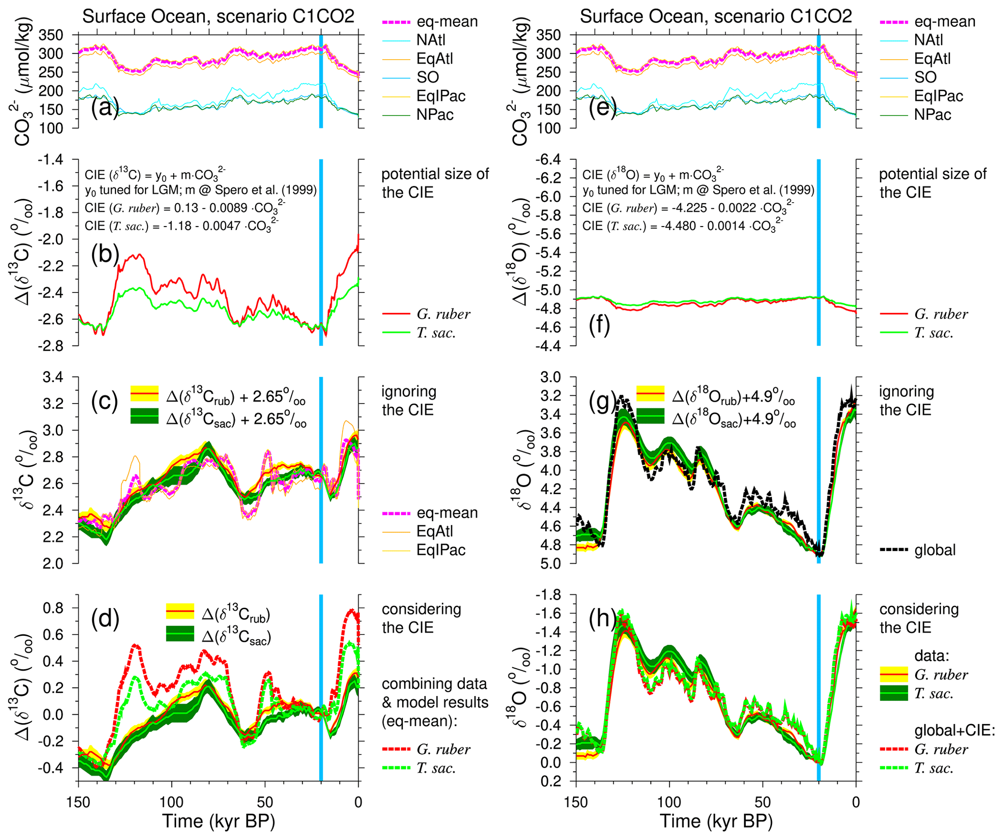
Figure 8 Calculating the suggested carbonate ion effects (CIE) on G. ruber and T. sacculifer. The left-hand column shows the effects on δ¹³C, while the right column shows the effects on δ¹⁸O. (a, e) Surface-ocean [CO${}_{\mathrm{3}}^{\mathrm{2}-}$]. (b, f) Potential CIE using slopes from Spero et al. (1999). (c, g) Surface-ocean conditions when ignoring the CIE or (d, h) when considering the CIE. Mean anomalies (±1 SE) of the isotope stacks are calculated with respect to the mean of 21–19 kyr BP (vertical blue band). Simulations use the results from scenario C1CO2. Different surface-ocean areas are distinguished: North Atlantic (NAtl; north of 50° N), equatorial Atlantic (EqAtl; 40° S–50° N), Southern Ocean (SO; south of 40° S), equatorial Indo-Pacific (EqIPac; 40° S–40° N) and North Pacific (NPac; north of 40° N). The mean wider tropical ocean in the model is the mean from the equatorial boxes (eq-mean).

3.4 Carbonate ion effect in δ¹⁸O

The focus of this study is on stable carbon isotope δ¹³C. However, during the construction of our mono-specific wider tropical stacks of Δ(δ¹³C_rub) and Δ(δ¹³C_sac), the corresponding stacks of Δ(δ¹⁸O_rub) and Δ(δ¹⁸O_sac) are easily generated by-products initially used to cross-check the applied age models. However, these δ¹⁸O data give us the possibility to also have a closer look at the role of the CIE in the recording of oxygen isotopes in foraminiferal shells. For that endeavour, we need a background time series of δ¹⁸O which represents the signals when not modified by the CIE. Such a mean δ¹⁸O in the wider tropical surface ocean should record the same sea-level-related variations as the average global ocean, but it might differ in the recorded temperature effect if the change in the average wider tropical sea surface temperature differed from the mean ocean temperature (MOT) change. Pöppelmeier et al. (2023) showed that the LGM-to-PRE change in the MOT derived from the model-based interpretation of noble gas reconstructions in ice cores is 2.1±0.7 K. The reconstructed rise in the MOT is slightly higher when ignoring the effect of past saturation changes on noble gases (Shackleton et al., 2023). The data assimilation effort in LGM temperature changes by Tierney et al. (2020) is broadly in agreement with the MOT change of Pöppelmeier et al. (2023) and proposes that the tropical (30° S to 30° N) sea surface was around 2.6 K colder at the LGM than at the PRE, agreeing within the uncertainties with the MOT change. To a first order, we therefore assume that the planktic foraminifera should record the same temperature effect in δ¹⁸O as contained in the mean ocean. Thus, the global ocean δ¹⁸O calculated from stacking benthic time series (Lisiecki and Stern, 2016) represents the CIE-free background against which we compare our new Δ(δ¹⁸O_rub) and Δ(δ¹⁸O_sac) stacks.

From the simulated LGM-to-PRE change in mean wider tropical surface-ocean CO${}_{\mathrm{3}}^{\mathrm{2}-}$ of about −70 µmol kg⁻¹ (Fig. 8e) and the laboratory-based amplitudes of the CIE (−0.0022 ‰ and −0.0014 ‰ change in δ¹⁸O per µmol kg⁻¹ for G. ruber and T. sacculifer, respectively (Spero et al., 1999)), we determined that Δ(δ¹⁸O_rub) and Δ(δ¹⁸O_sac) should record the changes since the LGM by +0.15 ‰ and +0.10 ‰ differently than how δ¹⁸O in the surface waters truly changed (Fig. 8f). Compared to the G-IG amplitude in mean ocean δ¹⁸O of −1.65 ‰ (Fig. 8g), these potential CIEs represent corrections of −9 % and −6 %, a difference of 3 % which might be difficult to detect in the paleo-records. A linear regression through a scatter plot of δ¹⁸O + CIE_rub versus δ¹⁸O + CIE_sac has a slope of 0.97 (r²=1.00; Fig. S8b), which is indistinguishable from the slope obtained from regression through the data stacks (Fig. 6b), while the slope when considering the CIE should move to unity (indicating that both species were recording the same signal underneath the CIE) if the effect plays an important role during data interpretation. The evidence for or against the CIE in δ¹⁸O from both data and models is therefore inconclusive.

4 Conclusions

The CIE for δ¹³C and δ¹⁸O recorded in planktic foraminifera was first identified in laboratory experiments (Spero et al., 1997, 1999), and it was, based on theory, suggested for both isotopes that the underlying processes are directly related to the pH in the surrounding seawater during hard-shell formation (Zeebe et al., 1999; Zeebe, 1999). However, these theoretical studies were already unable to confirm the full range of the CIE as contained in the experiments. Furthermore, according to Bijma et al. (1999), it is impossible to determine if pH or [CO${}_{\mathrm{3}}^{\mathrm{2}-}$] is responsible for the observed fractionation effects. If this theoretical understanding is correct, we would expect to see the CIE in neither or both isotopes in the our mono-specific stacks. Thus, although the interpretation of δ¹⁸O with respect to the CIE is uncertain due to the signal-to-noise ratio, we argue, based on the clear evidence of a lack of the CIE in the recording of δ¹³C in G. ruber and T. sacculifer, that there is probably also no significant CIE contained in the δ¹⁸O time series of both species. This finding argues against the suggestion of Spero et al. (1999) that the CIE and δ¹³C time series from G. ruber and T. sacculifer might be used to calculate a record of surface-ocean [CO${}_{\mathrm{3}}^{\mathrm{2}-}$]. Furthermore, we suggest using our new stack of Δ(δ¹³C_rub) as representative of δ¹³C_DIC in the wider tropical surface ocean.

Various possible explanations for the lack of a CIE on orbital timescales exist. Firstly, it might be that the isotopic fractionation during hard-shell formation in G. ruber and T. sacculifer is rather insensitive to [CO${}_{\mathrm{3}}^{\mathrm{2}-}$] in the range of interest (250–320 µmol kg⁻¹). Such an insensitivity has been suggested for other species (Bijma et al., 1999), but, due to a lack of published data (the slopes of the CIE in G. ruber and T. sacculifer were only summarised in Spero et al. (1999), while underlying experiments have never been published in the peer-reviewed literature), it cannot be properly checked for the two species investigated here. Secondly, not the CIE, but alternatively the incorporation of respired CO₂ (depleted in δ¹³C) during shell formation, might be responsible for the observed isotope data in laboratory experiments performed with Orbulina universa and Globigerina bulloides (Bijma et al., 1999). This process might also play a role in G. ruber and T. sacculifer, but it would only explain observed effects in δ¹³C and not in δ¹⁸O. However, since our stacks are inconclusive with respect to the CIE and δ¹⁸O, they might be of relevance here. A third explanation might be related to homeostasis. In symbiont-bearing planktic foraminifera, such as G. ruber and T. sacculifer, the pH at the shell surface critically depends on photosynthesis and hence light levels and symbiont density (Jørgensen et al., 1985). In order to facilitate calcification, G. ruber and T. sacculifer may actively influence the pH at the shell surface by seeking specific (optimum) light levels through vertical migration, thereby keeping the CIE constant over time. Planktic foraminifera are known to move vertically in the water column (e.g. Kimoto, 2015). Vertical migration to optimise both nutrient uptake and light has been proposed to play an important role in phytoplankton by modelling (Wirtz et al., 2022), an effect which has recently been supported by field data (Zheng et al., 2023). We speculate that similar behaviour could occur in the two planktic foraminifera species. Indeed, Jonkers and Kučera (2017) and Daëron  and Gray  (2023) found that δ¹⁸O in various planktic foraminifera (including G. ruber and T. sacculifer) is best explained by also considering calcification in waters deeper than their expected living depth.

It is too early to be able to generalise our finding that on orbital timescales the CIE plays no role in the interpretation of signals in planktic foraminifera in paleo-records. For that endeavour, more mono-specific stacks are necessary, preferably from conceptually different foraminifera species without symbionts or spines, as these might potentially show a different behaviour with respect to light (and pH) optimisation. However, our findings might suggest that previous studies on planktic δ¹³C, which ignored the CIE (e.g. Lynch-Stieglitz et al., 2019; Lund et al., 2019), might not be biased.

Our carbon cycle simulations confirm that atmospheric δ¹³CO₂ and mean surface-ocean δ¹³C_DIC are tightly related to each other, highlighting the importance of air–sea gas exchange for carbon isotopes. This is not entirely new, and it has already been discussed before (e.g. Lynch-Stieglitz et al., 2019; Shao et al., 2021; Pinho et al., 2023). However, the ¹³C cycle is more complex than stated previously (Lynch-Stieglitz et al., 2019; Hu et al., 2020; Pinho et al., 2023). These studies suggested that one might calculate a mean surface-ocean δ¹³C_DIC as a function of atmospheric δ¹³CO₂ and a temperature-dependent fractionation during gas exchange. We assumed here, based on modern data from Verwega et al. (2021), that species composition, and therefore isotopic fractionation during marine photosynthesis, might also be temperature-dependent, having an important impact on surface-ocean δ¹³C_DIC. Furthermore, our simulation results show that δ¹³C_DIC in polar oceans and in the wider tropical surface ocean have a different and time-dependent relation to atmospheric δ¹³CO₂.

Finally, since our simulations were forced by atmospheric carbon records, we are unable to identify specific processes being responsible for the simulated changes in the ¹³C cycle. Recent climate simulations (Yun et al., 2023) emphasise the importance of the 405 kyr eccentricity cycle in tropical hydroclimate. It therefore seems reasonable that the missing long-term variability in δ¹³C in our setup might indeed be connected to weathering fluxes, as proposed before (e.g. Schneider et al., 2013; Wang et al., 2014), something which needs to be tested in more detail in future carbon cycle simulation studies.

Appendix A

The following citations contain the original publications for the data used to produced our stacks. More details are found in Table S1: Adegbie et al. (2003); Adegbie (2001); Andres (2002); Arz et al. (1998); Arz et al. (1999a); Arz et al. (1999b); Ausin et al. (2019); Bostock et al. (2004); Chen et al. (2003); CLIMAP Project Members (1981); Curry and Crowley (1987); Curry et al. (1999); De Deckker et al. (2012); Duplessy (1982b); Duplessy et al. (1991); Dupont and Kuhlmann (2017); Dürkoop (1998); Dürkoop et al. (1997a); Dürkoop et al. (1997b); Dürkoop et al. (1997c); Dyez et al. (2014); Freimüller (2013); Ge et al. (2010); Gemmeke (2010); Gibbons et al. (2014); Gingele et al. (2007); Govil and Divakar Naidu (2011); Hale and Pflaumann (1999); Holbourn et al. (2005); Hou et al. (2020); Ivanova et al. (2003); Johnstone et al. (2014); Keigwin (2004); Kemle-von Mücke (1994); Knaack (1997); Knaack and Sarnthein (2005); Kohn et al. (2011); Koutavas and Lynch-Stieglitz (2003); Leech et al. (2013); Li et al. (2009); Li et al. (2010); Linsley (1996); Lo et al. (2017); Lynch-Stieglitz et al. (2015); Meinecke (1992); Michael et al. (1984); Mohtadi et al. (2010a); Mohtadi et al. (2010b); Mohtadi et al. (2011); Mohtadi et al. (2014); Monteagudo et al. (2021); Moros et al. (2009); Mulitza (1994); Mulitza (2009); Mulitza et al. (1999); Mulitza et al. (2022); Naik and Naidu (2016); Parker et al. (2016); Patrick and Thunell (1997); Paul et al. (2012); Portilho-Ramos et al. (2018); Raza et al. (2014); Richter (1998); Romahn (2014); Romahn et al. (2014); Rühlemann et al. (1996); Sarnthein et al. (1988); Sarnthein et al. (1994); Schefuß et al. (2005); Schneider (1991); Shackleton et al. (1992); Sirocko (1989); Sirocko et al. (2000); Slowey (1990); Slowey and Curry (1992); Spero et al. (2003); Stott et al. (2002); Stott et al. (2007); Tian et al. (2010); Tierney et al. (2017); Toledo et al. (2007); Vahlenkamp (2013); Venancio et al. (2018); von Rad et al. (1999); Wang et al. (1999); Wang et al. (2016); Wang et al. (2013); Wefer et al. (1996); Winn (2013); Zahn-Knoll (1986); Zimmermann (2013).