A multi-model assessment of the early last deglaciation (PMIP4 LDv1): a meltwater perspective

The last deglaciation (∼20–11 ka BP) is a period of a major, long-term climate transition from a glacial to interglacial state that features multiple centennial- to decadal-scale abrupt climate variations whose root cause is still not fully understood. To better understand this time period, the Paleoclimate Modelling Intercomparison Project (PMIP) has provided a framework for an internationally coordinated endeavour in simulating the last deglaciation whilst encompassing a broad range of models. Here, we present a multi-model intercomparison of 17 transient simulations of the early part of the last deglaciation (∼20–15 ka BP) from nine different climate models spanning a range of model complexities and uncertain boundary conditions and forcings. The numerous simulations available provide the opportunity to better understand the chain of events and mechanisms of climate changes between 20 and 15 ka BP and our collective ability to simulate them. We conclude that the amount of freshwater forcing and whether it follows the ice sheet reconstruction or induces an inferred Atlantic meridional overturning circulation (AMOC) history, heavily impacts the deglacial climate evolution for each simulation rather than differences in the model physics. The course of the deglaciation is consistent between simulations except when the freshwater forcing is above 0.1 Sv – at least 70 % of the simulations agree that there is warming by 15 ka BP in most places excluding the location of meltwater input. For simulations with freshwater forcings that exceed 0.1 Sv from 18 ka BP, warming is delayed in the North Atlantic and surface air temperature correlations with AMOC strength are much higher. However, we find that the state of the AMOC coming out of the Last Glacial Maximum (LGM) also plays a key role in the AMOC sensitivity to model forcings. In addition, we show that the response of each model to the chosen meltwater scenario depends largely on the sensitivity of the model to the freshwater forcing and other aspects of the experimental design (e.g. CO₂ forcing or ice sheet reconstruction). The results provide insight into the ability of our models to simulate the first part of the deglaciation and how choices between uncertain boundary conditions and forcings, with a focus on freshwater fluxes, can impact model outputs. We can use these findings as helpful insight in the design of future simulations of this time period.

1 Introduction

At the onset of the most recent deglaciation, ∼19 000 years before present (ka BP; year 1950 as present), ice sheets that covered the Northern Hemisphere at the Last Glacial Maximum (LGM; Dyke 2004; Lambeck et al., 2014; Hughes et al., 2016) started to melt (Gregoire et al., 2012), Earth began to warm (Jouzel et al., 2007; Buizert et al., 2018), and sea levels rose (Lambeck et al., 2014). Known as the “last deglaciation”, this time period is defined by major, long-term (order of 10 000 years) climate transitions from the most recent cold glacial to the current warm interglacial state, as well as many short-term, decadal- to centennial-scale warmings and coolings of more than 5 °C (de Beaulieu and Reille, 1992; Severinghaus and Brook, 1999; Lea et al., 2003; Buizert et al., 2018). These short-term abrupt temperature changes were often also accompanied by sudden reorganisations of basin-wide ocean circulations (e.g. Roberts et al., 2010; Ng et al., 2018) and jumps in sea level of tens of metres in a few hundred years (e.g. Deschamps et al., 2012; Lambeck et al., 2014).

Abrupt climate changes observed in the early last deglaciation, such as the Greenland cold period known as Heinrich Stadial 1 (between ∼18.5 and 14.7 ka BP; Broecker and Putnam 2012; Huang et al., 2014, 2019; Crivellari et al., 2018; Ng et al., 2018) and the Bølling Warming (an abrupt warming that occurs ∼14.7 ka BP in Greenland at the end of Heinrich Stadial 1; (Severinghaus and Brook, 1999; Lea et al., 2003; Buizert et al., 2018), are often attributed to changes in the Atlantic meridional overturning circulation (AMOC). The strength and structure of the ocean circulation is a key control on the North Atlantic and Arctic climate and is dependent on the stratification of the water layers in crucial convection sites in the North Atlantic (Lynch-Stieglitz et al., 2007; McCarthy et al., 2017). When the AMOC is strong, more heat is transported towards the North Atlantic, causing regional warming in Greenland and the North Atlantic (Rahmstorf, 2002).

Previous studies have shown that the AMOC pattern can be perturbed easily by changes in meltwater input into the North Atlantic. For example, if freshwater is deposited into the critical convection sites in the subpolar North Atlantic, i.e. the Labrador Sea and Nordic Seas, locations of high sensitivity to wind patterns and sea ice formation, the circulation strength can be disrupted (Rahmstorf, 1999). Evidence from several sites report sea level rise, and therefore a freshwater flux, as early in the deglaciation as 19.5 ka BP, attributed to widespread retreat of Northern Hemisphere ice sheets in response to an increase in northern latitude summer insolation (Yokoyama et al., 2000; Clarke et al., 2009). Carlson and Clark (2012) concluded that the LGM was terminated by a rapid 5–10 m sea level rise between 19.5 and 19 ka BP, and sea levels rose a further 8–20 m from ∼19 to 14.5 ka BP with the melting of the Laurentide and Eurasian ice sheets. More recent reconstructions of sea level and ice volume change suggest a similar view with ∼10–15 m of sea level rise between the end of the LGM (∼21–20 ka BP) and 18 ka BP and an additional ∼25 m before 14.5 ka BP (Lambeck et al., 2014; Peltier et al., 2015; Roy and Peltier, 2018; Gorbarenko et al., 2022). In some cases where meltwater fluxes are applied to the North Atlantic in model simulations, rapid decreases of up to 10 °C in temperature occur, resembling the transition to Heinrich Stadial 1 (e.g. Ganopolski and Rahmstorf, 2001; Knutti et al., 2004; Brown and Galbraith, 2016; Menviel et al., 2020).

Transient simulations of the last deglaciation have been increasingly performed to better understand the multi-millennial-scale processes and the shorter and more dramatic climate changes by examining dynamic and threshold behaviours (Braconnot et al., 2012), determining the effects of temporally varying climate forcings, and identifying what mechanisms in the model can cause recorded climate signals (see Sect. 1.2 of Ivanovic et al., 2016, and examples therein). In turn, these simulations also provide us with the opportunity to test the ability of models to simulate climate processes and interactions and different hypotheses for drivers of change (i.e. climate triggers, interactions, and feedbacks).

One particularly challenging aspect in the experimental design of last deglaciation simulations is prescribing ice sheet evolution and the resultant freshwater flux and sea level rise. Notwithstanding the qualitative rationale for why ocean-bound meltwater disrupts ocean circulation and climate (McManus et al., 2004; Clarke et al., 2009; Thornalley et al., 2010), it has been recently argued that climate models are too sensitive to freshwater fluxes under some conditions. For example, data reconstructions suggest only a small change in AMOC ∼11.7 to 6 ka BP, whereas CCSM3 (Community Climate System Model version 3) simulated a greater response to the freshwater forcing associated with the final Northern Hemisphere deglaciation at this time (He and Clark, 2022), when sea level rose by 50 m during this interval (Lambeck et al., 2014; Cuzzone et al., 2016; Ullman et al., 2016). This result may be quite model dependent, and we note that others had previously suggested the converse, i.e. that model responses to freshwater (and other) forcings could be too muted, from what we understand of past climate change (Valdes, 2011; Liu et al., 2014). Certainly, to disrupt climate in a Heinrich Stadial-like way, many previous glacial simulations have required quite large meltwater fluxes compared to what may be inferred from geological records (Kageyama et al., 2013). This remains an interesting point of contention (i.e. the meltwater paradox defined below), and certainly some models no longer appear as “stable” as they once did. Moreover, the sensitivity of the North Atlantic Ocean circulation to glacial melting is poorly constrained.

There are, however, strong indications that the impact of oceanic freshwater fluxes is highly dependent on the location that they enter the ocean (depth and latitude–longitude) and how they are implemented, as it determines the efficiency of convection disruption (e.g. Stocker et al., 2007; Roche et al., 2007, 2010; Smith and Gregory, 2009; Otto-Bliesner and Brady, 2010; Condron and Winsor, 2012; Ivanovic et al., 2017; Romé et al., 2022). Similarly, the background climate and ocean state may also be important for how responsive ocean circulation is to freshwater forcing – e.g. whether AMOC is already strong and deep or weak and shallow (Bitz et al., 2007; Schmittner and Lund, 2015; Dome Fuji Ice Core Project Members et al., 2017; Pöppelmeier et al., 2023b), or specifically where deep water formation occurs (Smith and Gregory, 2009; Roche et al., 2010). The choice of a model's boundary conditions in the paleo-setting (e.g. ice sheet geometry) can influence its sensitivity to freshwater perturbation. For example, the Romé et al. (2022) simulations have an oscillating AMOC, whereas the simulations by Ivanovic et al. (2018) do not, and Kapsch et al. (2022) demonstrated various climate responses in simulations of the last deglaciation with different ice sheets. Ice sheet geometry specifically has been demonstrated to affect AMOC strength due to the impact of ice sheet height on surface winds and wind-driven gyres, which can increase the northward transport of salty waters. Multiple model studies (e.g. Ullman et al., 2014; Löfverström and Lora, 2017; Sherriff-Tadano et al., 2018; Kapsch et al., 2022) have shown that a thicker Laurentide ice sheet results in a stronger AMOC. Hence, the influence of deglacial ice sheet meltwater on AMOC is likely to be highly dependent on the model, choice of boundary conditions and forcings, and the initial ocean condition.

Furthermore, CO₂ and orbital forcing are also shown to impact the course of the deglaciation and the occurrence of abrupt climate changes (i.e. results shown by Oka et al., 2012; Klockmann et al., 2016, 2018; Zhang et al., 2017; Sherriff-Tadano et al., 2018) and potentially modulate the sensitivity of the AMOC to freshwater fluxes (Obase and Abe-Ouchi, 2019; Sun et al., 2022). Liu et al. (2009) demonstrated that the warming in TraCE-21ka between 17 and 14.67 ka BP is dominated by the CO₂ forcing (over the orbital forcing; see their Fig. S6a), which coincides with the first major rise in atmospheric CO₂ in their simulation. Whereas Gregoire et al. (2015) demonstrated that orbital forcing caused 50 % of the reduction in North American ice volume, greenhouse gases caused 30 %, and the interaction between the two caused the remaining 20 % in their coupled climate–ice sheet simulations. Sun et al. (2022) showed the effect that these forcings have on the sensitivity of the AMOC, by demonstrating that a weak AMOC (in a Heinrich Stadial 1-like state, for example) is more likely to recover (like that of the Heinrich Stadial 1 to Bølling Warming transition) with a higher atmospheric CO₂ concentration and that larger ice sheets result in a stronger AMOC that is less sensitive to meltwater fluxes.

Previous modelling efforts (e.g. Liu et al., 2009; Roche et al., 2011; Menviel et al., 2011; Gregoire et al., 2012; He et al., 2021) performed transient simulations to learn more about the last deglaciation and the interaction between ocean and atmosphere. Liu et al. (2009) were the first to publish a synchronously coupled atmosphere–ocean general circulation model simulation of the last deglaciation, henceforth referred to as TraCE-21ka. In this study, a freshwater flux was used to regulate the AMOC to achieve a set of target ocean circulation, surface air temperature, and sea surface temperature conditions as interpreted from a selection of proxy records in multiple locations between the LGM and the onset of the Bølling Warming (see Fig. 1 by Liu et al., 2009), followed by a switch to a geologic reconstruction of freshwater forcing (He, 2011).

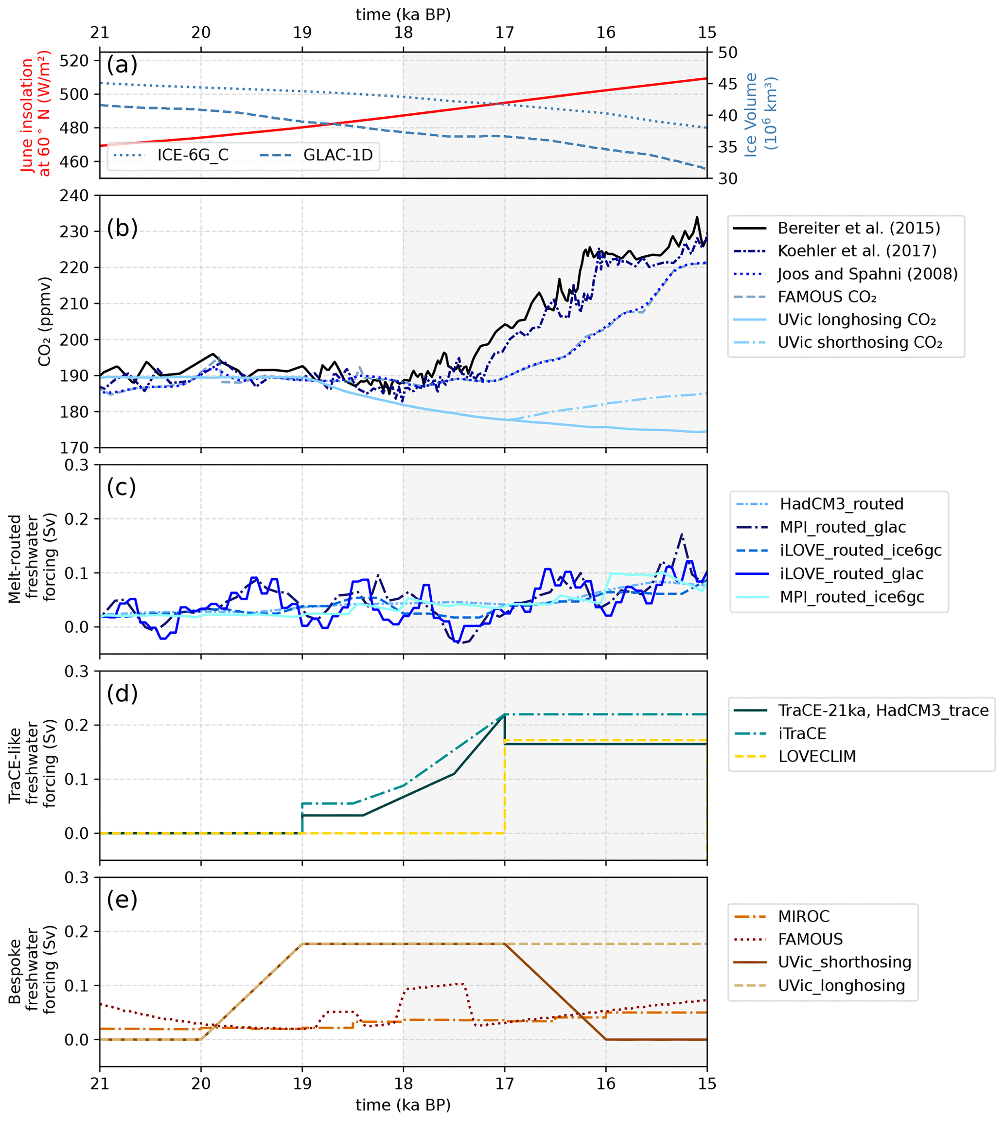
Figure 1 Climate forcings for the simulations. (a) Ice volume loss since the Last Glacial Maximum (LGM; 21 ka BP) as part of the ICE-6G_C ice sheet reconstruction (Argus et al., 2014; Peltier et al., 2015) and the GLAC-1D ice sheet reconstruction (Tarasov and Peltier, 2002; Tarasov et al., 2012; Briggs et al., 2014; Ivanovic et al., 2016) in light blue. June insolation at 60° N (Berger, 1978) is in red. (b) Atmospheric CO₂ concentrations are dependent on the simulation set-up. (c–e) Freshwater flux (Sv) for simulations with imposed meltwater. Melt-uniform simulations have the same total meltwater flux into the global ocean as melt-routed simulations (c), but in melt-uniform scenarios, the freshwater is spread through the entire ocean or across the whole ocean surface (see main text), rather than at point sources, and are hence so diluted or uniformly distributed as to have limited direct forcing power.

The meltwater inputs used in TraCE-21ka and the studies referenced above, however, do not follow ice sheet reconstructions (e.g. Ivanovic et al., 2018). Instead, the meltwater fluxes are, on occasion over twice as large as suggested by ICE-6G_C VM5a (henceforth “ICE-6G_C”; Argus et al., 2014; Peltier et al., 2015) and GLAC-1D (Tarasov and Peltier, 2002; Tarasov et al., 2012; Briggs et al., 2014; Ivanovic et al., 2016). Furthermore, the freshwater flux must then be shut off to reinvigorate the AMOC and instigate the Bølling Warming, ending Heinrich Stadial 1, but this is at the same time as recorded rise in global sea level of 12–22 m in ∼350 years or less, known as Meltwater Pulse 1a (Deschamps et al., 2012). Meltwater Pulse 1a is a complex event thought to be a culmination of contributions from the North American (Gregoire et al., 2012, 2016), Eurasian (Brendryen et al., 2020), and Antarctic (Weber et al., 2014; Golledge et al., 2014) ice sheets. Whilst some studies have suggested that freshwater in the Southern Ocean could have contributed to the temperature changes seen in the North Atlantic during the Bølling Warming, recent studies (e.g. Ivanovic et al., 2018; Yeung et al., 2019) have demonstrated that the impact of meltwater pulses in the Southern Ocean on the climate are often restricted to the Southern Hemisphere, whereas North Atlantic pulses have much farther-reaching and dominating affects. This creates a meltwater paradox, where the freshwater forcing required by models to produce recorded climate change is broadly in opposition to the meltwater history reconstructed from ice sheet and sea level records.

Simulations performed by Kapsch et al. (2022) and Snoll et al. (2022) add weight to this so-called meltwater paradox. They use meltwater forcing scenarios in accordance with observable ice volume change but have not been able to replicate the AMOC or surface air temperature proxy records. Instead, the AMOC remains stronger than ocean circulation records suggest for Heinrich Stadial 1, and the models simulate an abrupt cooling at ∼14.5 ka BP instead of the Bølling Warming. The picture is further confounded from the ice sheet modelling perspective (e.g. see Fig. S2 by Gregoire et al., 2012).

Similar simulations of the last deglaciation (e.g. Roche et al., 2011; Snoll et al., 2022; Bouttes et al., 2023) have been run with no prescribed meltwater or a meltwater forcing that is applied as a global salinity adjustment (i.e. rather than localised surface forcing). Without the use of the freshwater forcing, these simulations do not reproduce any abrupt climate change events during the deglaciation.

The simulation performed by Obase and Abe-Ouchi (2019) is unique in that it is able to simulate a weak AMOC during the onset of the deglaciation and the Bølling Warming without releasing (and then stopping) an unrealistically large amount of freshwater. Instead, they input a gradually increasing amount of meltwater that remains at or below the level of ice volume loss in the reconstruction. This study was able to simulate spontaneous abrupt changes in AMOC thanks to multi-stability in their ocean circulation, as also seen in other modelling studies (Romé et al., 2022; Malmierca-Vallet et al., 2023). This simulation still does not consider Meltwater Pulse 1a and has lower than observed meltwater input before that point, yet it is distinctive in its ability to replicate a weak ocean circulation in the early deglaciation and the Bølling Warming even with a continuous freshwater flux.

Despite the decades of research simulating the last deglaciation and numerous observable records of this time period, uncertainty still remains about the mechanisms that cause the recorded climate signals as well as how to replicate them “realistically” in model simulations, and therefore how to unravel the meltwater paradox. These findings highlight the importance of solving the convolved issue of model sensitivity to specific forcings and boundary conditions and the initial climate condition and model dependency of simulation results – the crux of the remaining unknowns. To tackle such unknowns, the Paleoclimate Modelling Intercomparison Project phase 4 last deglaciation protocol version 1 (PMIP4 LDv1; Ivanovic et al., 2016) was designed to encompass a broad range of models and the uncertainty in boundary conditions and forcings. Instead of one specific and rigid configuration for the experiment design, modelling groups are given a choice of recommended forcings and boundary conditions. Thus, analysing model output of multiple simulations of the last deglaciation provides the opportunity to look at differences between experimental designs and their impact on the onset of the deglaciation using different models.

This study compares 17 simulations of the last deglaciation from nine different climate models with dissimilar experimental designs. Our aim is to take advantage of the numerous simulations available to better understand the chain of events and mechanisms of climate changes in the early last deglaciation (i.e. from 20 to 15 ka BP) and our collective ability to simulate them. We focus on the early deglaciation because although models may start differently from the LGM, the divergence from each other is smaller in comparison to further into the deglaciation. We investigate the similarities and differences between the model results and what aspects of the variations in the model output can be attributed to the experimental design or model biases by analysing the transition from the LGM, when and where the warming starts, and the impact of freshwater forcing. We also address the meltwater paradox by discussing the results of meltwater scenario choices made by the modelling groups.

2 Experiment designs across the ensemble

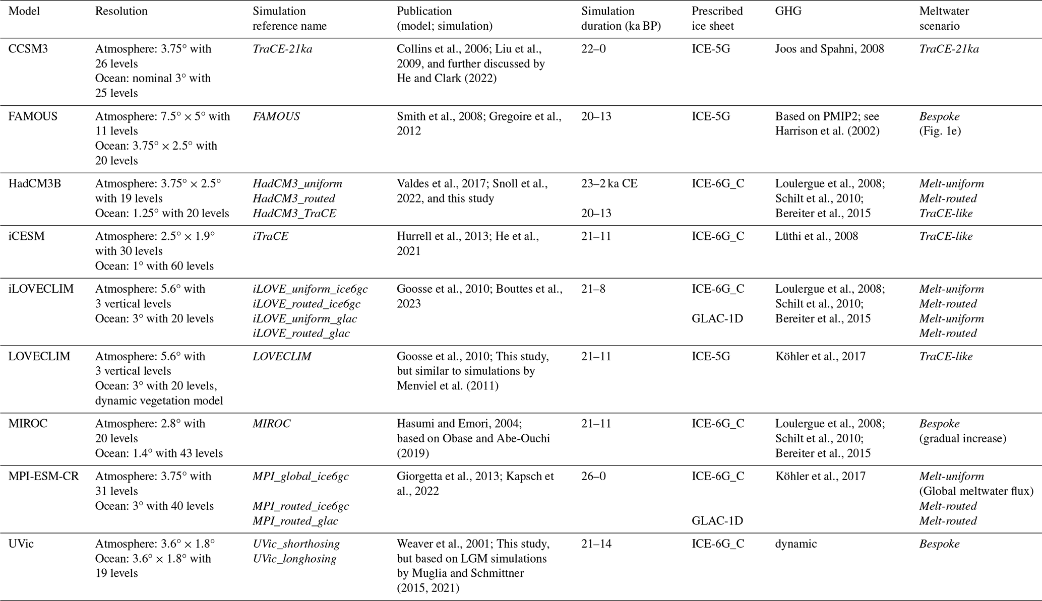
The comparison is based on 17 simulations produced independently by eight different palaeoclimate modelling groups using nine different climate models (Table 1). Most groups have followed the most recent PMIP4 last deglaciation protocol for their experimental design, while others use older publications for boundary conditions or a more bespoke configuration depending on their own modelling goals. The simulations from HadCM3, LOVECLIM, iLOVECLIM, iCESM, MIROC, and MPI modelling groups use greenhouse gas configurations on the AICC2012 age model of Veres et al. (2013) (Fig. 1b). FAMOUS and TraCE-21ka use an older age model in which the deglacial rise in CO₂ starts a thousand years later. The deglacial CO₂ concentration for these two models is almost identical, with some discrepancies between ∼19.8 and 18.4 ka BP and about 15.7 ka BP. All simulations prescribe insolation following Berger (1978) (Fig. 1a). The PMIP4 last deglaciation protocol recommends using the GLAC-1D (Ivanovic et al., 2016) and/or ICE-6G_C (Peltier et al., 2015) ice sheet reconstructions. HadCM3, iCESM, MIROC, and UVic modelling groups opted for ICE-6G_C; MPI and iLOVECLIM simulations use both ICE-6G_C and GLAC1-D; and FAMOUS, LOVECLIM, and TraCE-21ka use the older ICE-5G (Peltier, 2004).

Table 1 Detail of simulations referenced in the multi-model intercomparison.

Freshwater forcing across the ensemble is more complex. The PMIP4 last deglaciation protocol recommends two different meltwater scenarios (melt-routed and melt-uniform) based on ice volume change as calculated from the ice sheet reconstruction chosen by the modelling group (GLAC-1D and ICE-6G_C are recommended). The melt-uniform scenario is a globally uniform freshwater flux or salinity adjustment through time applied throughout the whole ocean to conserve water mass during deglaciation of the ice sheets, whereas the melt-routed scenario is a distributed routing that gives the flux of freshwater through time at individual meltwater river outlets along the coast (Ivanovic et al., 2016; Riddick et al., 2018 – used by MPI).

Because a large discrepancy between the simulations is the prescribed freshwater flux scenario (Fig. 1d–f), and ice sheet meltwater fluxes are known to have a major impact on ocean circulation and climate (see above), the simulations have been grouped into four categories based on their meltwater forcing: melt-routed, melt-uniform, those based on the TraCE-21 ka A simulation (henceforth referred to as TraCE-like; Liu et al., 2009), and bespoke scenarios that fall outside of the other three categories. Within these categories, however, there is variation in how the freshwater forcing is derived from the ice sheet reconstruction, as well as in the technical implementation of the chosen meltwater scenario (for example, for the melt-routed and melt-uniform scenarios, see Wickert, 2016, Sect. 2.2.2 for HadCM3; Kapsch et al., 2022; Sect. 2 for MPI; Bouttes et al., 2023, Sect. 2.4 for iLOVECLIM). For the melt-routed simulations, the modelling groups then release the calculated meltwater flux to ocean grid cells according to the distribution calculated by the individual groups' drainage network models (see the respective papers). For the melt-uniform simulations, HadCM3 and iLOVECLIM modelling groups apply a globally uniform freshwater flux throughout the entire volume of the ocean, whereas the MPI modelling group applies a freshwater flux at the surface of the ocean or land. Because of this nuance, the MPI melt-uniform simulation is instead labelled as a “global surface meltwater flux” but is still placed in the melt-uniform category for our analysis.

We somewhat over-simplistically refer to PMIP4 meltwater scenarios as “realistic” because they are based on the chosen ice sheet reconstruction prescribed in the simulation. Nonetheless, it is important to note that the precise history of the meltwater flux (distribution and rates) remains quite uncertain, as hinted at by differences in the reconstructions. Between 20 and 15 ka BP, the realistic freshwater flux according to ICE-6G_C does not exceed 0.1 Sv and according to GLAC-1D only exceeds 0.1 Sv as it nears Meltwater Pulse 1a. In the TraCE-like simulations, the strategy of prescribing freshwater to induce an inferred AMOC history requires the freshwater flux to reach nearly 0.2 Sv or greater – twice the realistic amount based on sea level records (Fig. 1d; Carlson and Clark, 2012; Lambeck et al., 2014).

For the bespoke-freshwater cluster of simulations, MIROC implements a gradually increasing flux that always remains below the realistic values. FAMOUS uses a reconstructed flux based on an earlier estimate from sea level records (produced as part of the ORMEN project; more information provided by Gregoire, 2010), which follows the more up-to-date ice sheet reconstructions relatively closely except when a larger freshwater flux is applied at two points during Heinrich Stadial 1 (between 19 and 17 ka BP; corresponding to the acceleration of Northern Hemisphere ice loss, as noted by Carlson and Clark, 2012, and the melt of the Eurasian ice sheet as reconstructed by Hughes et al., 2016). The UVic simulations use a total freshwater flux calculated as 3 times the sea level changes reconstructed by Lambeck et al. (2014); one scenario where the freshwater flux is applied between 19 and 15 ka BP (Uvic_longhosing) and one where the flux is only applied between 19 and 17 ka BP (Uvic_shorthosing; Table 1).

The UVic simulations include a dynamic carbon cycle model with prognostic atmospheric CO₂ aiming to replicate the sedimentary records of deep-ocean carbon. The freshwater flux is therefore tuned to replicate the AMOC structure associated with these sedimentary records, but the location of the meltwater input is based on plume positions like those of the HadCM3 simulations. The UVic simulations are included in the broader comparisons presented here (i.e. Fig. 3). However, because of their unique experiment design and motivation, the differences between the UVic simulations and the wider multi-model ensemble are too great for a more detailed comparison of results, and they are therefore omitted from parts of the analysis and discussion in this study.

3 Analysis method

One of the analyses used in this study was inspired by the year of first significant warming analysis performed by Roche et al. (2011). We define the first significant warming from the LGM using a statistical test. The LGM reference period is selected from the 500-year window between 21 and 20.5 ka BP for each simulation. Each of the simulations are then divided into 65 independent samples of 100 years between 20.5 and 13 ka BP for each grid cell. For each sample, we first performed a Fischer test on the variances in the reference and test samples to assess whether they differed or not. If the variances were equal, we performed a standard one-sided Student's t test with the alternative hypothesis as the sample period being warmer than the reference LGM period. If the variances were not equal, we performed a Welsch's test, or a t test with two unequal variances with the same alternative hypothesis. The samples were tested at 99 % confidence. If the sample was significantly warmer than the LGM reference period, then the grid point in Fig. 5 was assigned the central point of this sample. For example, if the 100-year sample between 16.2 and 16.1 ka BP at a specific grid point was determined to be significantly warmer than the reference period, then that grid point would be assigned the year 16.15 ka BP). This analysis excludes two of the simulations (HadCM3_TraCE and iTraCE) due to data availability before 20 ka BP. LOVECLIM was also not included due to a small drift between 21 and ∼20.6 ka BP because of an adjustment in the ice sheet. This analysis was performed for all simulations with an earlier reference period (20–19.5 ka BP) and shown in the Supplement. The remaining analyses in this study use a LGM definition of 20 to 19.5 ka BP to incorporate all simulations.

Two temporal correlations are also performed between AMOC and surface air temperature and CO₂ concentration and surface air temperature. For both relationships, a R² value and slope of a linear regression model is calculated at each grid cell for the 5000-year window from 20 to 15 ka BP.

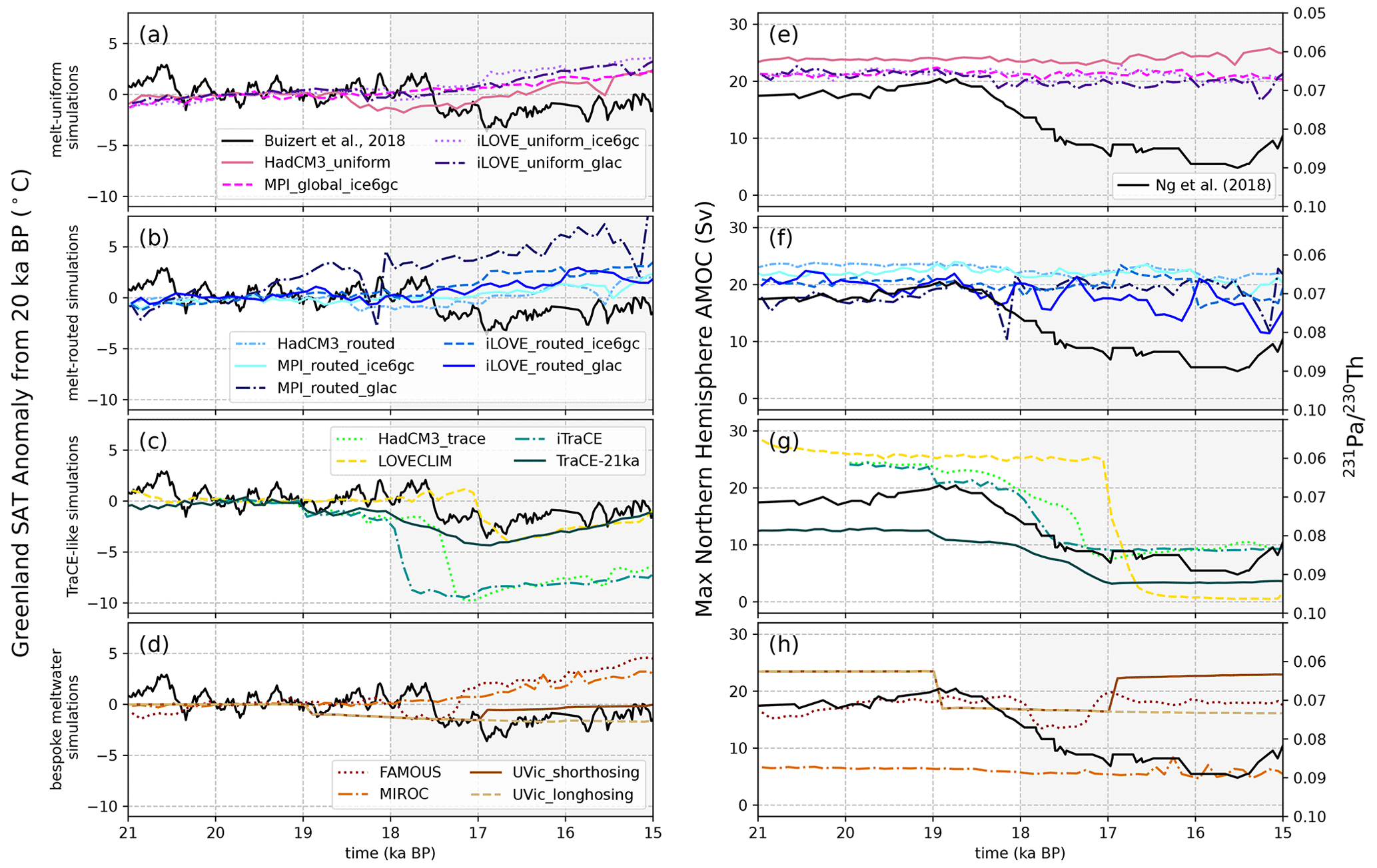
Figure 2 Centennial means for (a–d) Greenland (between 65 and 82° N and 30 and 55° W) surface air temperature anomaly from approximately the LGM (20–19.5 ka BP) for each simulation. (e–h) Maximum AMOC of the Northern Hemisphere at depth between 500 and 3500 m. For comparison, (a–d) includes Greenland surface air temperature proxy record from Buizert et al. (2018), plotted as an anomaly from 20 ka BP in black, and (e–h) includes the AMOC proxy ${}^{\mathrm{231}}\mathrm{Pa}{/}^{\mathrm{230}\mathrm{Th}}$ composite record published by Ng et al. (2018), plotted in black (note the arbitrary y-axis scaling). The grey-shaded region denotes the timing of Heinrich Stadial 1.

4 Results and discussion

Here, we focus on the course of the deglaciation, how it is impacted by the freshwater forcing, and how this relationship differs on a model-to-model and experimental design-to-experimental design basis. The trajectory of the AMOC in the Northern Hemisphere for each simulation closely follows the meltwater scenario chosen by the modelling group (Fig. 2). All the melt-routed, melt-uniform, and bespoke freshwater scenarios display a similar pattern throughout the deglaciation with a gradual warming of surface air temperature in the high latitudes and stronger warming compared to the TraCE-like simulations in the Northern Hemisphere (Fig. 3). The similarity between the simulations increases further into the deglaciation, with warming from the LGM in all regions by 16 ka BP for all the melt-routed, melt-uniform, and bespoke freshwater scenarios (Figs. 3 and S1 in the Supplement). The TraCE-like simulations, however, do not follow the same trajectory, and the Northern Hemisphere, specifically the North Atlantic, remains colder than at the LGM for most of the early deglaciation, with only LOVECLIM and TraCE-21 ka warming beyond the LGM in the North Atlantic by 15 ka BP (Fig. S2). This colder region in the North Atlantic is evident in a multi-model mean of the ensemble where, on average, the North Atlantic remains the coldest region throughout the early deglaciation (Fig. 4). Around the onset of Heinrich Stadial 1 (18 ka BP), more discrepancy between simulations arises (as indicated by disagreement even in the sign of change; Fig. 4) due to differences across the ensemble in when and where the deglaciation begins as well as the freshwater fluxes applied. However, by 15 ka BP, at least 70 % of simulations agree with the sign of the mean in most areas. More disagreement remains in the North Atlantic, the region of highest variance across the ensemble and where the different freshwater fluxes used in the simulations have the most direct impact. The ensemble-wide consensus of a warming climate, however, is consistent with the increases in North Hemisphere summer solar insolation and atmospheric CO₂ (Fig. 1a and b).

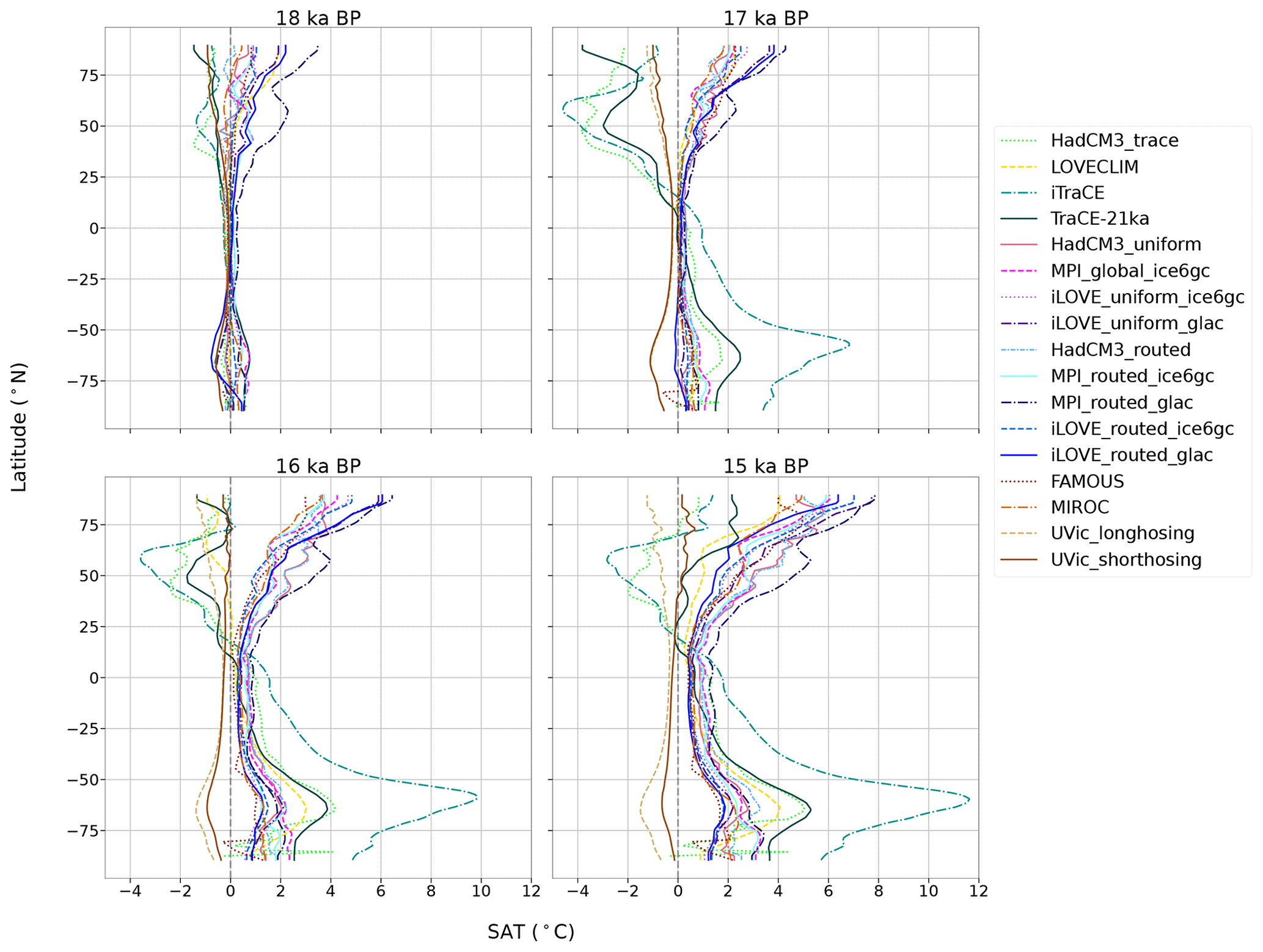
Figure 3 Zonal average of decadal mean surface air temperature as anomalies from the LGM (20–19.5 ka BP) for each simulation; 18, 17, 16, and 15 ka BP are calculated as 60-year decadal means centred around the respective time period (e.g. from 17.97 to 18.03 ka BP for 18 ka BP).

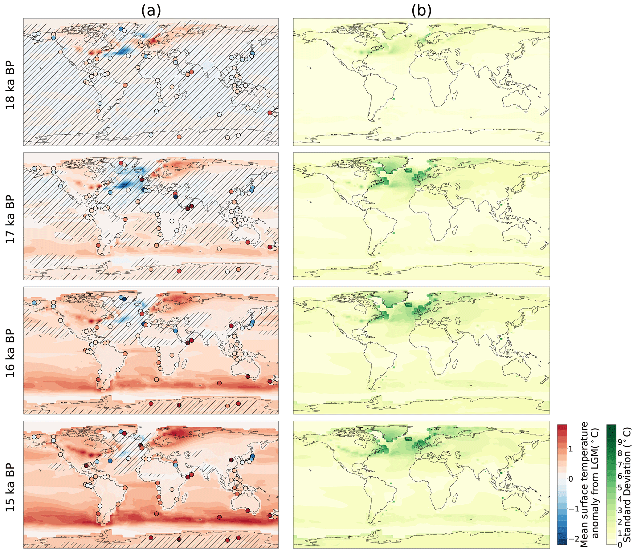
Figure 4 (a) Multi-model mean of decadal surface temperature anomaly from the LGM (20–19.5 ka BP) at each time step labelled (not including the UVic simulations). Hatching denotes areas in which less than 70 % of the simulations agree with the sign of the mean. The agreement with the sign of the mean was determined using a one sample t test at 95 % confidence by testing if the simulation and the mean were both significantly different from zero in the same direction. Column (b) is the same as column (a) but showing the variance. Filled circles show the proxy surface temperature stack from Shakun et al. (2012) on the same colour scale; 18, 17, 16, and 15 ka BP are calculated as 60-year decadal means centred around the respective time period (e.g. from 17.97 to 18.03 ka BP for 18 ka BP).

4.1 Timing of the deglaciation

Between 20 and 15 ka BP, each of the meltwater groups, except for the TraCE-like simulations, have relatively constant AMOC strengths. The melt-uniform simulations show the least millennial-scale variability in AMOC (Fig. 2e). The melt-routed simulations, in comparison, have more variation, aligned with the respective freshwater fluxes, and show a weakening trend starting at ∼16.5 ka BP as freshwater input increases towards Meltwater Pulse 1a (Fig. 2f; Meltwater Pulse 1a at 14.7 ka BP not shown). Like the melt-routed simulations, the bespoke simulations have more change that is consistent with the freshwater flux, but for all bespoke simulations except for UVic_longhosing, the AMOC strengths at 21 ka BP and at 15 ka BP are very similar.

The subset of TraCE-like simulations, on the other hand, show an abrupt weakening in AMOC strength and an associated decrease in Greenland surface air temperature (anomaly from LGM, calculated as anomalies from the 500-year time window from 20–19.5 ka BP) beginning between 18 and 17 ka BP depending on the simulation (Fig. 2c and g). The differences in the timing of the decrease in temperature for the TraCE-like simulations are likely associated with the differences in timing and magnitude of the freshwater flux. For instance, iTraCE shows an earlier and more abrupt cooling than TraCE-21ka. Despite both simulations reaching the same magnitude of freshwater at 17 ka BP, the rate of freshwater input into the simulation between 19 ka BP and 17 ka BP differs. At 19 ka BP, there is a larger increase in the freshwater flux in iTraCE, which corresponds to a smaller but rapid decrease in the AMOC strength and Greenland surface air temperature at this same time. After 19 ka BP, the freshwater flux in iTraCE remains higher than in TraCE-21ka, and this is consistent with the sharper decrease in surface air temperature in iTraCE in comparison to the relatively steady decrease in temperature in TraCE-21ka.

HadCM3_TraCE uses the same meltwater scenario as TraCE-21ka, but instead of a gradual response, there is a more abrupt decrease in the Greenland surface air temperature at ∼17.5 ka BP and temperatures drop. The drop is as low as in iTraCE (with respect to the LGM) and occurs after the freshwater flux has decreased for both TraCE-21ka and HadCM3_TraCE. However, note that TraCE-21ka and HadCM3_TraCE are configured with different boundary conditions (i.e. HadCM3_TraCE uses greenhouse gas conditions on the AICC2012 timescale and the ICE-6G_C ice sheet reconstruction, whereas the CCSM3 TraCE-21ka simulation uses ICE-5G) with the exclusion of the freshwater forcing. Other simulations with similar boundary conditions to HadCM3_TraCE (i.e. HadCM3_routed) and TraCE-21ka (i.e. FAMOUS), but different freshwater forcings, do not show the large and abrupt decrease in the Greenland surface air temperature. This suggests that the freshwater forcing is a dominant driver of the abrupt changes displayed in both simulations; however, the differences between them might contribute to the differences in sensitivity to the meltwater flux.

In addition, although the meltwater scenario for LOVECLIM is based upon TraCE-21ka, the freshwater flux begins later, at 17 ka BP. Presumably because of this, the decrease in surface air temperature and AMOC strength is also delayed until 17 ka BP. The freshwater input is also much more abrupt in comparison to TraCE-21ka and iTraCE, corresponding to the rapid transition in the AMOC and surface air temperature at 17 ka BP. The implications of these differences amongst the simulations in the TraCE-like meltwater group are further described in Sect. 4.4.

The GLAC-1D ice sheet reconstruction has more variable meltwater input in comparison to ICE-6G_C, at least partly due to the more frequent updates of the ice sheet geometry and associated boundary conditions (every 100 years compared to every 500 years; Fig. 1a). This more variable meltwater forcing is evident in the higher variability of the AMOC strength and Greenland surface air temperature (Fig. 2b and f; e.g. the sharp decline and subsequent increase in temperature and AMOC strength at ∼18.5 ka BP in MPI_routed_glac that occurs at the same time as an increase in meltwater release).

All the simulations that do not follow the TraCE-like meltwater forcing follow a similar trajectory throughout the deglaciation with a gradual warming of surface air temperature in Greenland, except for the UVic simulations. The UVic simulations differ presumably because of the bespoke freshwater flux that ends earlier than the end of Heinrich Stadial 1 for the short-hosed simulation and after Meltwater Pulse 1a for the long-hosed simulation. The resultant impacts on the dynamically simulated carbon cycle causes atmospheric CO₂ concentrations to decrease during AMOC weakening, which contradicts reconstructions of this time period (e.g. Bereiter et al., 2015; Ng et al., 2018). Hence, in UVic_longhosing, decadal surface air temperature remains cold throughout the onset of the deglaciation, and UVic_shorthosing does not begin to warm in the Northern Hemisphere until the freshwater hosing is turned off at 17 ka BP (Fig. 2).

In most simulations, significant warming from the LGM (see Sect. 3 for how this is defined) occurs in most locations by 19 ka BP except in parts of the tropics where significant warming does not occur until as late as 16–17 ka BP (Fig. 5). The earlier warming in the high northern latitudes is likely associated with the increase in insolation (Fig. 1a; CAPE-Last Interglacial Project Members, 2006; Park et al., 2019; Kapsch et al., 2021) and the impact of polar amplification, whereas the warming in the tropics is more delayed and correlates with the timing of CO₂ concentration increase (Figs. 1b and S3a–d). The mean pattern is aligned with the results from Roche et al. (2011) (see Fig. 4 by Roche et al., 2011) that similarly show an earlier warming in the northern and southern high latitudes and delayed warming in the tropics. The effect of the freshwater forcing on the global temperature, however, was not incorporated in the no-melt simulations from Roche et al. (2011). Nevertheless, in the TraCE-like simulations, the meltwater impact is evident by the strong cold anomalies in the North Atlantic, the region where most of the freshwater forcing is applied or drained into (Figs. 3 and 4). Therefore, warming in this region, despite initially occurring at the onset of the deglaciation, is halted until much later in comparison to the other simulations (as further evident in the discussion around Fig. S3).

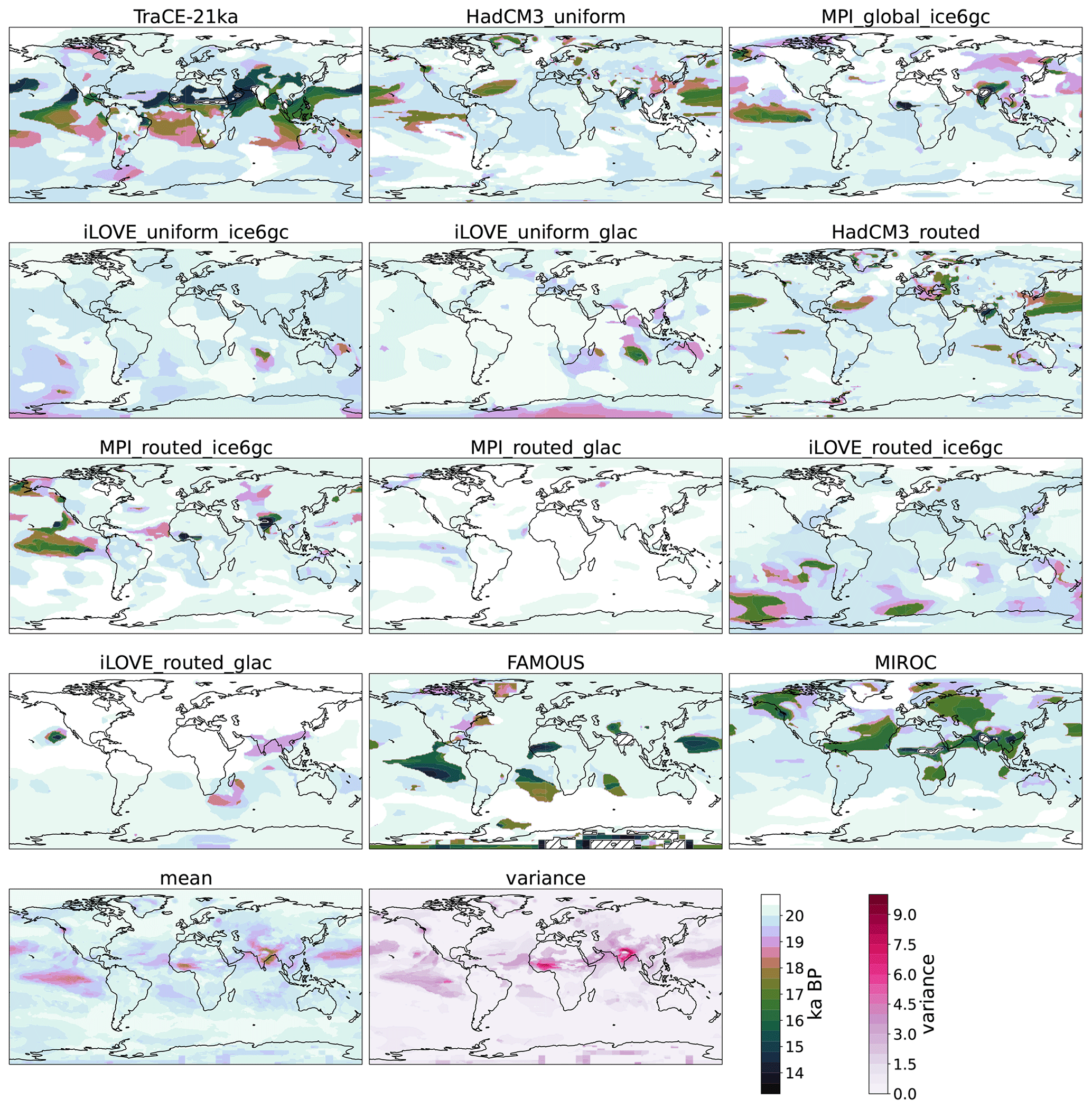
Figure 5 Year of first significant warming from 20 ka BP, where “significant warming” is determined as discussed in Sect. 3. Hatching denotes where significant warming did not occur before 13 ka BP.

This dissimilarity in the trajectory of warming is also evident in global surface air temperature anomalies from the LGM (Figs. 4 and S1). Early in the deglaciation, at 18 ka BP, there is disagreement between simulations as to the timing and magnitude of the warming as well as to which regions. For instance, MPI_routed_glac has warmed ∼4 °C in the North Atlantic by 18 ka BP, whereas MIROC still has colder regions throughout the tropics and Pacific with respect to the LGM (20–19.5 ka BP) and has only started to warm in the high latitudes, most likely associated with insolation increases (Fig. S1).

The iLOVECLIM and MPI simulations have significant warming in most areas from the immediate onset of the deglaciation, with MPI_routed_glac displaying the earliest significant warming globally compared to the other simulations (Fig. 5). Similarities are also evident amongst simulations that use the same model but different meltwater scenarios, e.g. between HadCM3_uniform and HadCM3_routed and between MPI_routed_ice6gc and MPI_global_ice6gc. The HadCM3 simulations have a matching cooling region around the Labrador Sea and Gulf Stream, and the MPI simulations have a matching cooling region in the Nordic Seas that each persist until ∼16 ka BP (more detail in Sect. 4.3). UVic remains unique amongst the simulations assessed in this study because between 20 and 15 ka BP most regions do not warm from the LGM. The CO₂ increase begins to take precedent in UVic_shorthosing after 17 ka BP and the melting ice sheets in North America and Fennoscandia show familiar warming patterns in the Northern Hemisphere for ICE-6G_C. This pattern, warming along the edges of the Northern Hemisphere ice sheets, is also evident in the other simulations using ICE-6G_C.

Despite the disagreements with the timing of the deglaciation on an individual scale, the sign of the multi-model mean of decadal surface temperature shares close agreement with the surface temperature stack produced by Shakun et al. (2012), and this is most significant in the Southern Hemisphere (Fig. 4). The median point-by-point difference between the multi-model mean and the proxy data is less than 1 °C between 18 and 15 ka BP, with a median of only 0.015 °C at 18 ka BP that increases to 0.993 °C by 15 ka BP, indicating that the multi-model mean of the ensemble replicates the Shakun et al. (2012) proxy stack relatively well but that disagreement with the proxy record grows further into the deglaciation. The largest discrepancies between the model output and reconstruction occur in the North Atlantic and Greenland (after 18 ka BP), which are also areas of more disagreement across the model ensemble (Fig. S4). This is the region where there are the most proxy records and therefore potentially the location in which the deglacial climate evolution is the best constrained (at least compared to the Pacific sector, for example). The North Atlantic is also the region where most models would show agreement for similar AMOC change; however, these simulations show various AMOC evolutions. It remains to be thoroughly tested if simulations that fit the constraints of the North Atlantic also fit the constraints of climate records from other locations. The multi-model mean tends to be cooler than the proxy data in the Southern Hemisphere but is warmer in many locations in the Northern Hemisphere (i.e. parts of the North Atlantic, Alaska, and off the coast of Japan). Interestingly, although the TraCE-like meltwater group represents the cold areas of the North Atlantic well, those simulations have difficulty replicating the warmer core locations in this same region. Conversely, the other meltwater groups present the opposite difficulty – they are better at replicating the warmer regions of the North Atlantic while failing to represent the cold ones (not shown). This suggests the potential need for subsequent investigations of broader model structure and how we interpret reconstructions (i.e. specific data points).

For the comparison to individual simulations, the surface temperature stack from Shakun et al. (2012) is compared to surface temperature change from the LGM in Fig. S1. Model–data comparison has also previously been performed by many of the individual modelling groups in their respective studies (see Table 1).

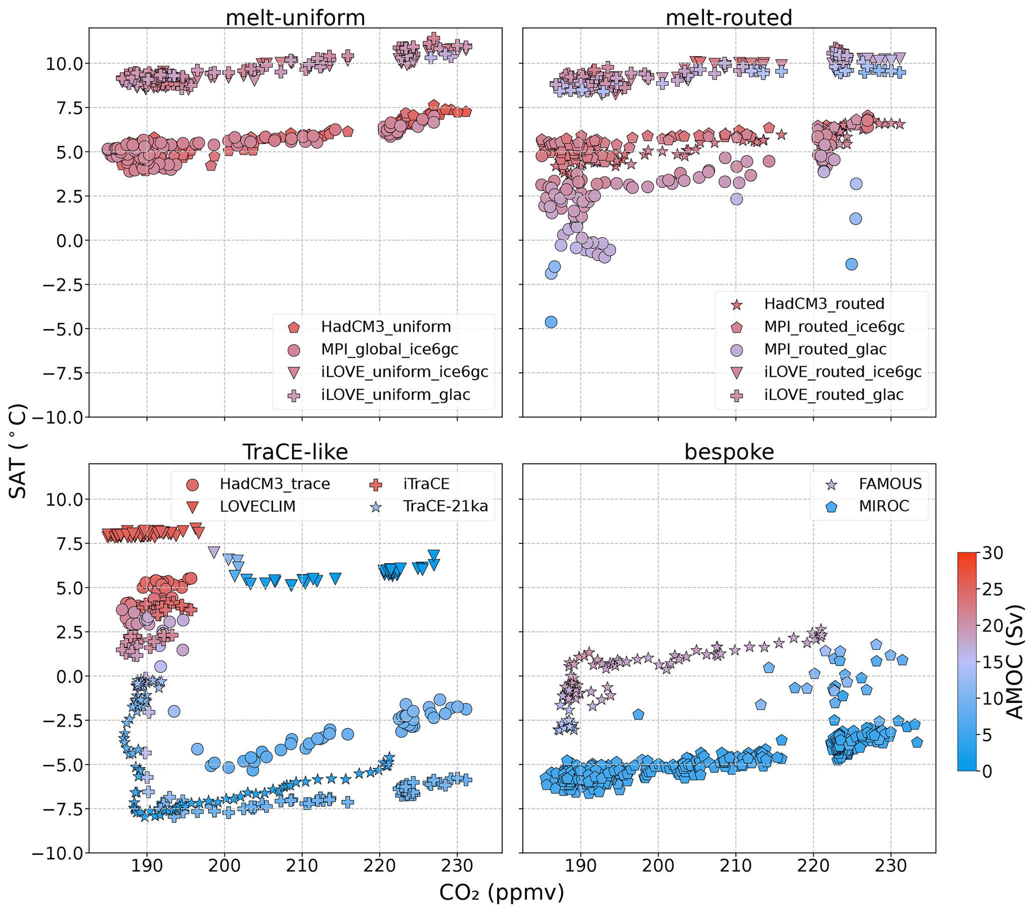
Figure 6 Absolute surface air temperature over the North Atlantic (between 35 and 60° N and −60 and 0° E) as a function of CO₂ concentration with symbol shading representing the strength of the AMOC (Sv) split into groups defined by meltwater scenario. The 50-year means are shown for each simulation except for MIROC, for which decadal means are shown to capture its temporally finer-scale variability. See Fig. S6 for the same analysis displayed as anomalies from 20 ka BP.

4.2 Linking surface climate, ocean circulation, and greenhouse gas forcing

In every simulation, there is the expected interrelation between surface air temperature in the North Atlantic, CO₂ concentration, and AMOC. As CO₂ increases, surface air temperature increases, as demonstrated by the increasing trends on each panel of Fig. 6. Surface air temperature is also higher when the AMOC is stronger, clearly shown by LOVECLIM. The simulations with smaller AMOC variation have a clearer relationship with CO₂ concentration (see melt-uniform panel and all the melt-routed simulations except for MPI_routed_glac; Fig. 6). The TraCE-like simulations each have a strong L-shaped curve in the relationship between CO₂ concentration and surface air temperature. This is because the initial large decrease in North Atlantic surface air temperature, representing Heinrich Stadial 1, occurs whilst the CO₂ concentration is relatively constant (Fig. 1b). However, after ∼18 ka BP (timing dependent on the CO₂ record used by the modelling group), CO₂ concentration begins increasing alongside a slow surface air temperature increase in each simulation.

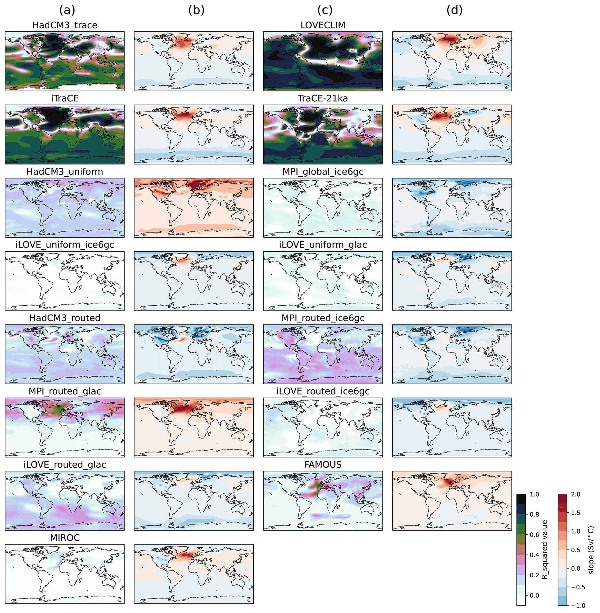
Figure 7 Spatial distribution of the temporal correlation of AMOC strength and surface air temperature using a linear regression model for the time period 20–15 ka BP using decadal means. Columns (a) and (c) show R² values as a result of the linear regression. Columns (b) and (d) show corresponding slopes to simulations in column (a) or (c) as a result of the linear regression.

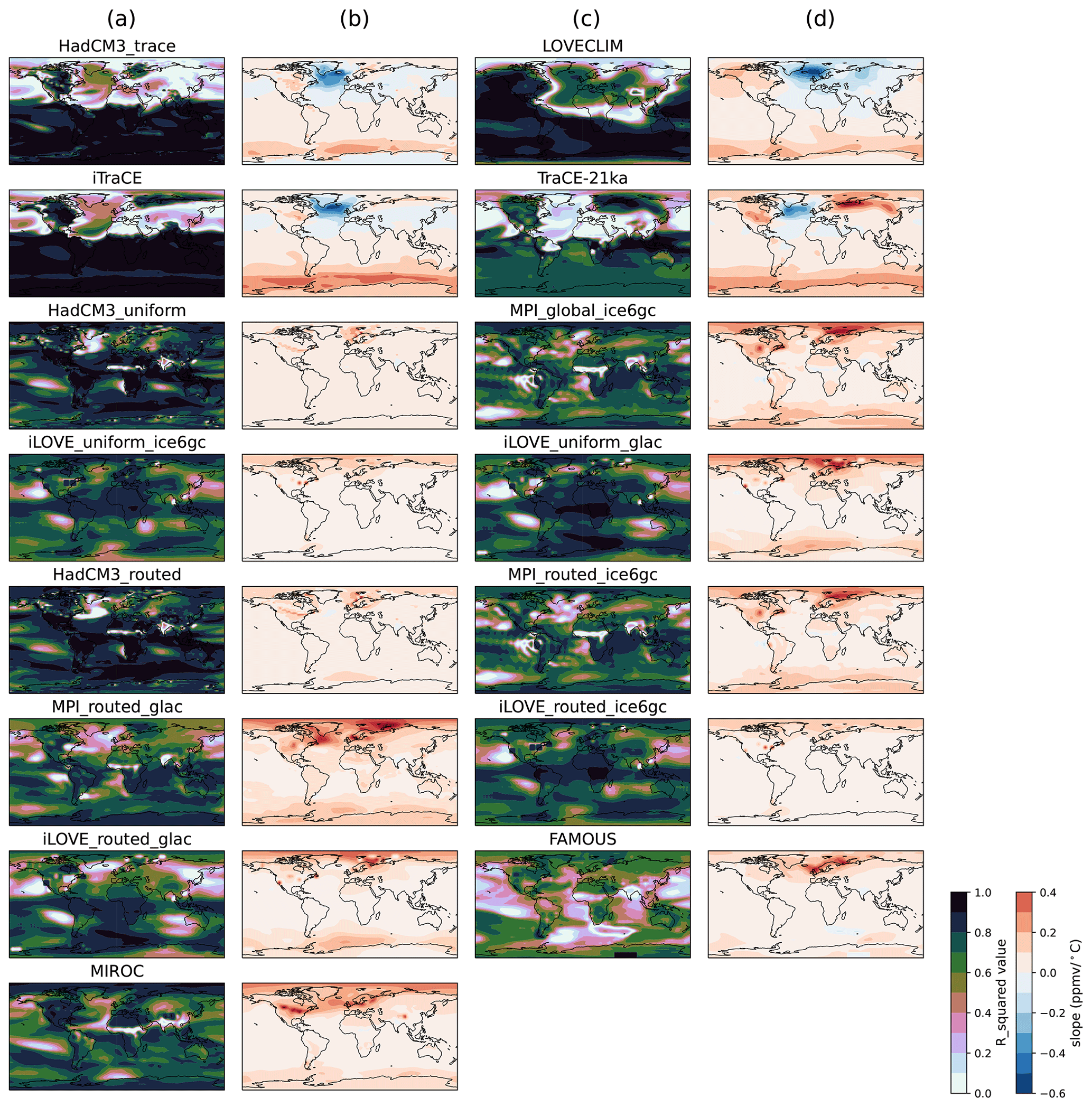
Figure 8 Spatial distribution of the temporal correlation of CO₂ concentration and surface air temperature using a linear regression model for the time period 20–15 ka BP using decadal means. Columns (a) and (c) show R² values as a result of the linear regression. Columns (b) and (d) show corresponding slopes to simulations in column (a) or (c) as a result of the linear regression.

The relationship between AMOC, CO₂, and surface air temperature is illustrated further by the R² values determined by a linear regression model across the entire period between 20 and 15 ka BP on a decadal temporal scale with surface air temperature as the dependent variable (Figs. 7 and 8). The results from the linear regression show that during the period of 20 to 15 ka BP, surface air temperature in the TraCE-like simulations has a stronger positive correlation with AMOC, and the other simulations in the ensemble have a stronger positive correlation with CO₂. For instance, the TraCE-like simulations have higher R² values between AMOC and surface air temperature in the North Atlantic than the other meltwater groups, presumably because changes between AMOC and surface air temperature correspond in the TraCE-like simulations between 20 and 15 ka BP, whereas the other simulations have a stable ocean circulation and very little temperature change during this time period (Fig. 2). FAMOUS, which has a stronger freshwater forcing between 20 and 15 ka BP in comparison to the other non-TraCE-like simulations, also has higher R² values between AMOC and surface air temperature in the North Atlantic region, though these are dampened relative to those of the TraCE-like simulation. The simulations with little AMOC and surface air temperature change show very low correlations between the two variables throughout the globe (e.g. iLOVECLIM simulations, the ICE-6G_C MPI simulations, and MIROC). However, the melt-routed GLAC-1D simulations, in comparison to their ICE-6G_C same-model counterparts, exhibit higher correlations. The correlation between AMOC and surface air temperature in MPI_routed_glac increases in the Irminger Sea and Nordic Seas from no correlation (R² is 0) in MPI_routed_ice6gc to an R² value of ∼0.6. The slope of the GLAC-1D simulation also changes from negatively correlated in most locations to positively correlated. The differences between the iLOVECLIM GLAC-1D and ICE-6G_C simulations are much smaller; The iLOVE_routed_glac simulation does display higher R² values in the Southern Hemisphere and some locations in North America and south of Greenland; however, this correlation is still low (below 0.5). The slopes between the simulations are also very similar. The larger differences in the MPI simulations could be due to the higher sensitivity of the simulations to the GLAC-1D freshwater flux, as described in more detail in Sect. 4.3.

The positive slope in the North Atlantic region for the TraCE-like simulations demonstrates the positive correlation between AMOC and surface air temperature changes, whereas the rest of the globe has a more negative correlation in most simulations, regardless of their meltwater group. This relationship is representative of the bipolar seesaw. The TraCE-21ka simulation most clearly exhibits this bipolar connection between the Northern Hemisphere and Southern Hemisphere with a strong positive correlation between AMOC and surface air temperature in the North Atlantic and a strong negative correlation in the Southern Ocean.

The relationship between CO₂ and surface air temperature (Fig. 8) in the Northern Hemisphere is nearly opposite to the relationship between AMOC strength and surface air temperature (Fig. 7) for HadCM3_TraCE, iTraCE, and TraCE-21 ka, with the areas of strong and positive correlation between AMOC and surface air temperature showing weaker and negative correlation between CO₂ and surface air temperature. This suggests that in the early deglaciation, if the AMOC is weakening or already weak because of the freshwater forcing when CO₂ starts to rise, the impact of CO₂ might be dampened or postponed in the Northern Hemisphere, whereas a strong correlation with surface air temperature remains in the Southern Hemisphere. The relationship between CO₂ and surface air temperature should be positive everywhere, so the negative correlation in the North Atlantic for the TraCE-like simulations proposes that the AMOC has a stronger influence than CO₂ during the studied period (20–15 ka BP) and that the regression analysis cannot properly separate the effects of AMOC and CO₂ for this type of experiment. The simulations with weaker correlation between CO₂ and surface air temperature in regions of the tropics (e.g. FAMOUS and parts of Sub-Saharan Africa in MIROC, MPI_global_ice6gc, and HadCM3_routed) also display delayed warming in these same locations (Fig. 5). Increases in obliquity are shown to delay warming in the tropics, specifically in these same parts of Africa as well as India, potentially due to increased cloud coverage and therefore cooling (Erb et al., 2013). In addition, the lag between the start of the CO₂ concentration increase (∼18 ka BP or later depending on the timescale used) and the insolation increase (∼20 ka BP) can disrupt the correlation between CO₂ and surface air temperature and create a localised delay in warming of the tropics (as also demonstrated in Fig. 5). Note that the analysis in Figs. 7 and 8 only goes until 15 ka BP, whereas the analysis in Fig. 5 reaches until 13 ka BP. The simulations with the very weak correlations between AMOC and surface air temperature (iLOVECLIM, MPI simulations, and MIROC) demonstrate globally high correlations with CO₂ except for a few concentrated regions. These regions of lower correlation are similar between simulations run by the same model and could indicate changes in upwelling strength during this time period.

It is important to note, however, that during the chosen time period only the TraCE-like simulations have strong and corresponding changes in the AMOC and surface air temperature. The suggested relationships could be checked by continuing this study through the later parts of the deglaciation to encompass greater amplitudes of change in the non-TraCE-like simulations.

4.3 Impact of different climate and ice sheet forcings and boundary conditions on model output

In this study, we include multiple simulations from the HadCM3, MPI, and iLOVECLIM modelling groups. These three modelling groups tested different PMIP4 boundary condition and forcing options: for example, implementing the melt-routed or melt-uniform scenario for the same ice sheet and/or using different ice sheets and associated meltwater scenarios (Table 1). Experimenting with the range of options the PMIP4 protocol enables us to review the impact of different climate forcings on the resultant model output.

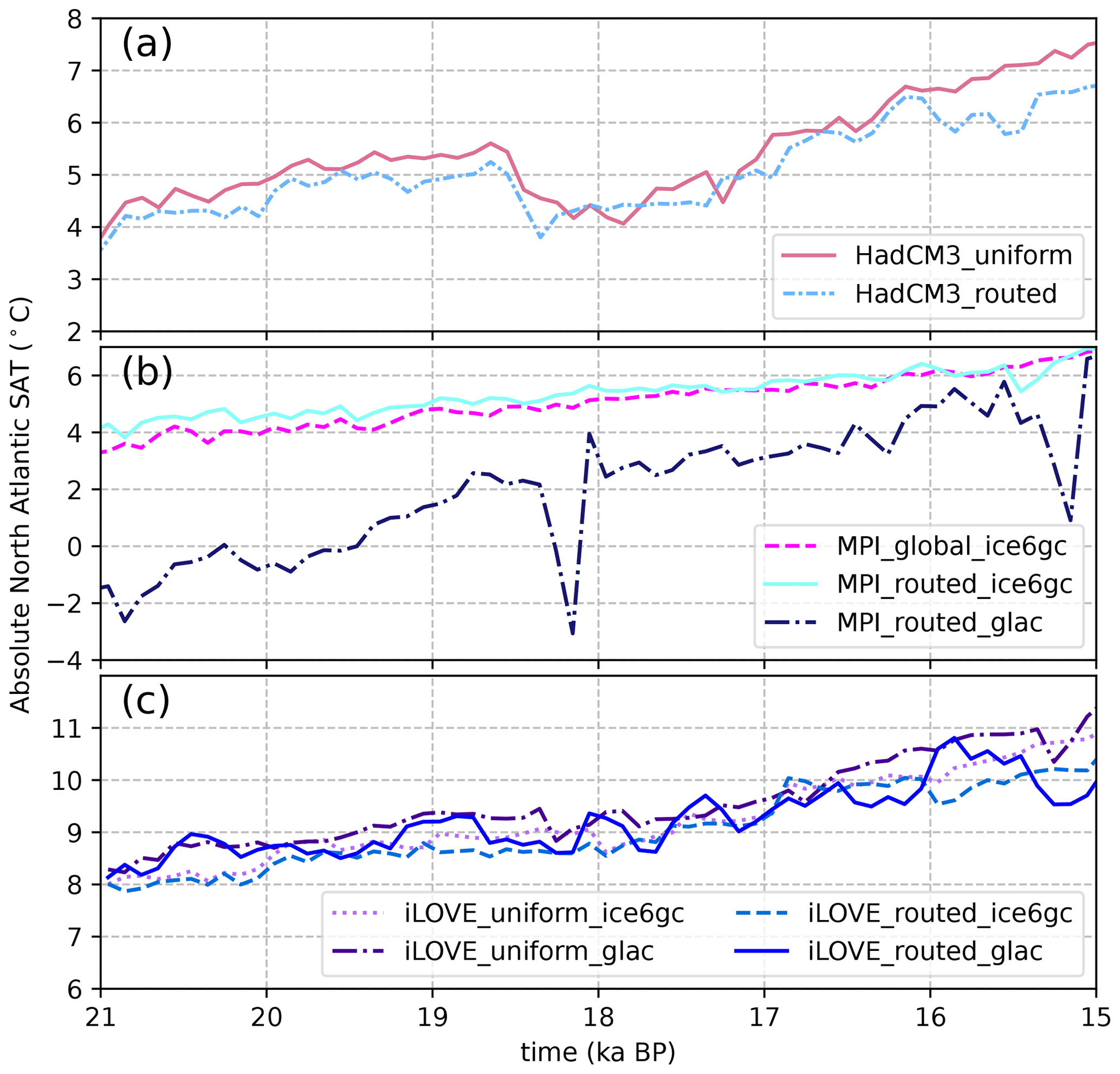
Figure 9 Absolute surface air temperature in the North Atlantic (between 35 and 60° N and −60 and 0° E) for the HadCM3, MPI-ESM, and iLOVECLIM simulations. Note that to capture variability, the y-axis limits are not the same for each panel. Absolute surface air temperature in the North Atlantic for the entire ensemble is shown in Fig. S5e–h.

The AMOC for each of the HadCM3, MPI, and iLOVECLIM simulations is impacted by the chosen meltwater scenario during the deglaciation (see Sect. 4.1). However, between 21 and 15 ka BP, the differences between the AMOC trajectory appear to be less affected by the meltwater scenario and are instead more significantly affected by the choice of ice sheet reconstruction (Figs. 2e–h and 9). For instance, when we compare the simulations with the different meltwater scenarios, but with the same ice sheet reconstruction (e.g. ICE-6G_C), i.e. HadCM3_uniform and HadCM3_routed, iLOVE_uniform_ice6gc and iLOVE_routed_ice6gc, and MPI_global_ice6gc and MPI_routed_ice6gc, we notice multiple similarities between the deglaciation trajectory both spatially and temporally. For instance, the HadCM3 simulations begin at a very similar surface air temperature in the North Atlantic at the start of the deglaciation (∼4 °C at 21 ka BP) and follow a comparable warming trajectory until 15 ka BP (reaching ∼7 °C; Fig. 9) despite the application of different meltwater scenarios, though the melt-routed simulation does remain colder in the North Atlantic than the melt-uniform simulation throughout the time period. In addition, spatially, as anomalies from the LGM (Figs. 3 and S1), the simulations look almost indistinguishable. Both display surface air temperature cooling along the Gulf Stream, and warming in locations of ice sheet melt, such as the Eurasian ice sheet in Fennoscandia and at the edge of the Laurentide ice sheet in North America. The most evident difference between the simulations is that HadCM3_uniform is colder than HadCM3_routed in the Labrador Sea and warmer in the Norwegian Sea, corresponding with differences in sea ice concentration – HadCM3_uniform has a higher sea ice concentration in the Labrador Sea than HadCM3_routed and a lower concentration in the Norwegian Sea (Fig. S7a and b). This pattern also corresponds to the dissimilarities in the convection sites between the two simulations as the melt-uniform simulation has more convection further south, along the sea ice edge, and in the Norwegian Sea, whereas the mixed-layer depth in the melt-routed simulation is deeper in the Labrador Sea (Fig. S7c). HadCM3_TraCE has the same dipole pattern as the other HadCM3 simulations, with cooling along the Gulf Stream and into Greenland and the Labrador Sea and warming over Fennoscandia; however, this signal is weak compared to the strong cooling in the North Atlantic due to the larger freshwater forcing applied.

Likewise, MPI_global_ice6gc and MPI_routed_ice6gc both begin at ∼4 °C at the start of the deglaciation in the North Atlantic and then warm at a comparable rate, but slower than the HadCM3 simulations, warming ∼3 °C by 15 ka BP rather than ∼5 °C. The MPI simulations, like the HadCM3 simulations, also share a similar spatial pattern with an area of strong cooling in the Nordic Seas and stronger warm patches off the coast of north-western North America and in the North Sea (Fig. S1). This pattern appears to be independent of the ice sheet reconstruction because MPI_routed_glac has the same areas of relative cold and warmth at 18 ka BP, but the signal is weaker, likely because MPI_routed_glac is ∼5 °C colder in the North Atlantic at the start of the deglaciation than the ICE-6G_C simulations and warming from the LGM occurs at a faster rate. Temporally, however, MPI_routed_glac displays more surface air temperature variability in the North Atlantic with abrupt climate changes as large as 5 °C and AMOC decreases of ∼9 Sv at ∼18.2 and 15.2 ka BP, most likely following the higher-frequency variability in the meltwater input from the GLAC-1D ice sheet reconstruction (Figs. 1c and 2) but also because MPI_routed_glac is significantly colder at the LGM compared to its ICE-6G_C counterparts. Kapsch et al. (2022) showed that the MPI simulations that are colder during the LGM lie closer to a critical threshold of AMOC variability. This aligns with the findings of Oka et al. (2012) and Klockmann et al. (2018) that demonstrate that the AMOC becomes more sensitive to perturbations, such as ice sheet topography and the resultant wind stress and CO₂ concentrations, when it is closer to an existing temperature threshold. Absolute surface air temperatures in the North Atlantic (Fig. S4e–h) show that multiple simulations in the ensemble are colder than MPI_routed_glac at the LGM, but only MIROC's AMOC appears to be close to a critical threshold of variability, as indicated by the changes in maximum AMOC strength towards 15 ka BP.

iLOVE_routed_glac has a similar, but less pronounced, variability of the AMOC and corresponding decreases in Greenland surface air temperature to MPI_routed_glac (Fig. 2b). However, in the North Atlantic, neither the iLOVE_routed_glac simulation nor iLOVE_uniform_glac exhibit significantly more variability than the ICE-6G_C iLOVECLIM simulations (relative to MPI_routed_glac and its ICE-6G_C counterparts). Spatially, the ICE-6G_C and GLAC-1D simulations are also nearly indiscernible (Fig. S1), except at the beginning of the deglaciation in the Southern Hemisphere, where surface air temperatures remain cooler for longer in the GLAC-1D simulations. This suggests that under these background conditions iLOVECLIM is less sensitive to freshwater perturbations than MPI-ESM-CR. This is dependent, however, on how both modelling groups calculate their freshwater flux, which can vary despite using the same ice sheet reconstruction (see Sect. 3), as well as, and potentially more importantly, the fact that these simulations are performed with two very different models. For example, iLOVECLIM is an Earth system model of intermediate complexity (EMIC) with three atmospheric layers (see Table 1), whereas MPI-ESM-CR is an Earth system model (ESM) with 31 atmospheric levels and thus can represent topographic feedbacks on the atmosphere with higher complexity and at finer-scale resolution.

Unfortunately, more simulations using a GLAC-1D-derived freshwater flux do not exist to compare to MPI_routed_glac and iLOVE_routed_glac and to get more robust results. Using GLAC-1D with the MPI model demonstrates more abrupt and higher reactivity to meltwater changes than the ICE-6G_C equivalents; however, this is less clear in the iLOVECLIM GLAC-1D simulations. Further simulations from other model types using both ice sheet reconstructions would be beneficial to understanding whether the systematic differences between the models contribute to the differences in sensitivity to the freshwater forcing. Otherwise, the simulations performed with the same model and ice sheet reconstruction display many similarities in the deglacial transition between 20 and 15 ka BP despite having different meltwater forcing scenarios.

4.4 Sensitivity of climate models to similar forcing(s)

All simulations, with the exclusion of the UVic simulations, TraCE-21 ka, and FAMOUS, use the greenhouse gas forcing on the AICC20212 timescale, with an increase in atmospheric CO₂ concentration at ∼17.5 ka BP. In contrast, in TraCE-21ka and FAMOUS, the CO₂ concentration does not begin increasing until ∼17 ka BP. This delayed increase in CO₂ postpones the warming of the deglaciation in these simulations, as is evident in the tropical regions (Figs. 3, 5, and S3). MIROC, despite not having a delayed CO₂ increase, also displays delayed warming in the tropics, like that of FAMOUS. This could be due to the higher sensitivity of MIROC to orbital forcing, causing it to take precedent over the CO₂ forcing earlier in the deglaciation (Obase and Abe-Ouchi, 2019).

Contrasting sensitivities of the models used for the TraCE-like simulations are evident in the response of the AMOC to the freshwater forcing and corresponding changes in Greenland surface air temperature in the different models (Fig. 2). By 17 ka BP, all four simulations have reached a similar and constant freshwater flux (with iTraCE ∼0.05 Sv, or 33 %, higher). The four simulations, however, begin with a range of different AMOC strengths. LOVECLIM has the strongest LGM AMOC at ∼28 Sv, TraCE-21ka with the weakest LGM AMOC at ∼12 Sv, and HadCM3_TraCE and iTraCE are in the middle of the cluster, starting with an AMOC strength of ∼24 Sv (see Sect. S4; Fig. 2g). Note that HadCM3_TraCE and iTraCE start at 20 ka BP, whereas LOVECLIM and TraCE-21ka start at 21 and 22 ka BP, respectively.

Despite beginning the deglaciation with the strongest AMOC, LOVECLIM's ocean circulation is also the most sensitive to the freshwater perturbation, causing its AMOC to crash to the weakest AMOC state of all the simulations (Fig. 2g). The temperature change in the LOVECLIM simulation, however, is comparable to the temperature change in TraCE-21ka despite the very different AMOC responses to the freshwater forcing. The AMOC collapses to nearly 0 Sv, but Greenland surface air temperature only decreases by ∼5 °C.

The Greenland surface air temperature response in HadCM3_TraCE and iTraCE appears to be impacted similarly by the change in AMOC strength, with both simulations following comparable trajectories throughout the deglaciation despite iTraCE having a larger freshwater flux. Both simulations exhibit an AMOC decrease of ∼14 Sv and $\sim -\mathrm{7}$ °C of temperature change between 19 and 16 ka BP. In addition, although TraCE-21ka and HadCM3_TraCE use the exact same freshwater flux, the HadCM3_TraCE simulation exhibits a decrease in AMOC strength of over ∼14 Sv and a corresponding decrease in surface air temperature of ∼10 °C in Greenland, whereas TraCE-21ka's AMOC strength weakens by only ∼9 Sv and Greenland surface air temperature only decreases by ∼4 °C. This suggests that the HadCM3 simulation is more sensitive to freshwater perturbations than TraCE-21ka but also that under the simulated climate conditions Greenland surface air temperature in HadCM3 is also more sensitive to corresponding AMOC changes compared to the other models. Additional exploration would be interesting to determine what different aspects between HadCM3_TraCE and TraCE-21ka could be contributing to the discrepancies in sensitivity (e.g. whether it could be the initial conditions, other boundary conditions, parameter choices, or simply model structure). The lower sensitivity of CCSM3 to freshwater perturbations is further investigated by He and Clark (2022) by rerunning TraCE-21ka but with no freshwater input during the Holocene. This version of the simulation is in better agreement with proxy Holocene AMOC kinematic reconstructions (McManus et al., 2004; Lippold et al., 2019).

The differences in model sensitivity are less observable in the simulations that apply meltwater forcing in accordance with the PMIP4 protocol's ice sheet consistent recommendations, as discussed in Sect. 4.3. Whereas the use of very similar freshwater fluxes amongst the TraCE-like simulations allows for easier comparison of changes in AMOC strength and corresponding surface air temperature. We determine that LOVECLIM's AMOC is the most sensitive to freshwater perturbations and that Greenland surface air temperature in HadCM3_TraCE is most sensitive to corresponding AMOC compared to other simulations in the TraCE-like meltwater group. Further simulations from other model types would be beneficial to determine what different aspects between the simulations could be contributing to the sensitivities.

4.5 Meltwater paradox

There has been ongoing debate on how much meltwater to input into simulations of the last deglaciation, and these results highlight the impact of the decision. The debate has stemmed from a so-called “meltwater paradox” that exists between the choice of large and geologically inconsistent meltwater forcings that successfully produce abrupt climate events versus glaciologically realistic meltwater fluxes that do not. This paradox is particularly evident in the last deglaciation during Heinrich Stadial 1 (between ∼18.5 and 14.7 ka BP) and the Bølling Warming (∼14.7 ka BP). Heinrich Stadial 1, for instance, is associated with weak ocean circulation strength (Lynch-Stieglitz, 2017; Ng et al., 2018; Pöppelmeier et al., 2023a) and cold climate conditions in multiple regions. There has been difficulty reconciling a weak AMOC in model simulations of the early deglaciation with the small amount of realistic freshwater release, as determined by the ice sheet reconstructions. Because of this, some model experiments (e.g. simulations in the TraCE-like meltwater group) have, by design, required overly large quantities of freshwater forcing to collapse their initially strong AMOCs and produce an abrupt cooling event such as that shown by surface air temperature proxy records (e.g. Wang et al., 2001; Ma et al., 2012). Ivanovic et al. (2018) suggested that the AMOC weakening targeted in these simulations is too large and that a smaller meltwater flux inducing more modest North Atlantic change may be sufficient to drive the recorded Heinrich Stadial climate. However, fully transient simulations that include only meltwater that is consistent with the ice sheet reconstructions (i.e. HadCM3_routed, MPI_routed_ice6gc, MPI_routed_glac, iLOVE_routed_ice6gc, iLOVE_routed_glac, and their corresponding melt-uniform simulations) do not achieve either the AMOC change or the surface climate signal of Heinrich Stadial 1.

In this context, the MIROC last deglaciation simulation is unique because it simulates a weak AMOC and cold surface air temperatures of Heinrich Stadial 1 (Figs. 2h and S3h) and the resumption of the AMOC of the Bølling Warming without releasing an unrealistically large amount of freshwater (not shown as this paper only covers until 15 ka BP; see Obase and Abe-Ouchi, 2019; Obase et al., 2021). Instead, a cold, weak-AMOC state is achieved with a gradually increasing meltwater flux that remains below the ice volume loss in the reconstruction and is used to regulate the timing of the abrupt resumption of the AMOC. The MIROC ocean circulation, therefore, displays a different sensitivity to freshwater input compared to the rest of the last deglaciation ensemble. This is likely in part due to the very weak LGM AMOC state at the start of the simulation, which also plays a role in the surface air temperature response and may make the simulation more susceptible to a small freshwater flux.

There is debate on the strength of the LGM AMOC and how this initial state impacts the subsequent climate change of the deglaciation. Some observations have suggested a weaker and shallower LGM AMOC than present day (e.g. Lynch-Stieglitz et al., 2007; Böhm et al., 2015; Lynch-Stieglitz, 2017), with agreement from recent data–model comparison studies (e.g. Menviel et al., 2017; Muglia and Schmittner, 2021; Wilmes et al., 2021; Pöppelmeier et al., 2023a). Other ocean circulation proxy studies (e.g. McManus et al., 2004; Gherardi et al., 2005, 2009; Ivanovic et al., 2016; Ng et al., 2018) demonstrated a consensus of a vigorous but shallower AMOC coming out of the LGM (relative to the modern day) that subsequently weakened and shallowed (but remained active; Bradtmiller et al., 2014; Repschläger et al., 2021; Pöppelmeier et al., 2023a) during the abrupt transition to Heinrich Stadial 1. Recent modelling studies have also suggested conditions between a deep and strong ocean circulation at the LGM (e.g. Menviel et al., 2011; He et al., 2021; Sherriff-Tadano and Klockmann, 2021; Kapsch et al., 2022; Snoll et al., 2022) due to the presence of thick ice sheets (Oka et al., 2012; Sherriff-Tadano et al., 2018; Galbraith and de Lavergne, 2019) and a shallow AMOC of similar strength to present day (e.g. Gu et al., 2020; Zhu et al., 2021).

As MIROC is the only PMIP4 last deglaciation simulation (LDv1 or previous) to simulate a weak ocean circulation at the onset of the deglaciation and then a later rapid resumption even with a continuous freshwater flux, this simulation may offer important insight to the conditions under which abrupt deglacial climate change may occur. Nonetheless, even this model cannot reproduce the Heinrich Stadial-Bølling Warming transition under Meltwater Pulse 1a-like freshwater forcing. Thus, the meltwater paradox of the last deglaciation remains.

This brings into question whether our models have the right sensitivity to freshwater fluxes. There appears to be a consensus as to the overall climate response to meltwater input in models and proxy records, i.e. the AMOC rapidly weakens, the North Atlantic cools, and sea ice forms, with the converse occurring when meltwater input stops. However, there is still less understanding and less agreement about how the AMOC responds to climate forcings. Because models appear to have AMOCs that are too stable, it is challenging to test both the AMOC response to a climate forcing and the climate response to an AMOC change at the same time. If a modelling group is interested in the response of the global climate to changes in the AMOC, they may be more inclined to adjust the meltwater pattern to trace the AMOC reconstruction, whereas if a modelling group is interested in the response of AMOC to a climate forcing, they may prefer to use the meltwater derived from the ice sheet reconstruction.

5 Conclusion

This study presents results from 17 simulations of the early part of the last deglaciation (20–15 ka BP) performed with nine different climate models. Our analyses show the first assessment of these simulations and display the similarities and differences between the model results as shown through the timing of the deglaciation, spatial and temporal surface air temperature changes, the link between the surface climate, ocean circulation, and CO₂ forcing, as well as how the different models respond to different forcings. The impact of the chosen meltwater scenario on the model output is evident in each result of this multi-model intercomparison study. The course of the deglaciation is consistent between simulations except when the freshwater forcing is above 0.1 Sv – at least 70 % of the simulations agree that there is warming by 15 ka BP in most places excluding the location of meltwater input. However, for simulations with freshwater forcings that exceed 0.1 Sv from 18 ka BP, warming is delayed in the North Atlantic and surface air temperature correlations with AMOC strength are much higher. The impacts of CO₂ forcing and increasing insolation (i.e. ice sheet melt and surface temperature warming) are reduced by the large freshwater fluxes imposed, delaying the warming in the Northern Hemisphere for these simulations. Nonetheless, the average of the ensemble displays the high latitudes beginning to deglaciate first in response to insolation and polar amplification and later warming occurring in the tropics in correlation with the rising CO₂ trajectory. The timing of the rise in CO₂ concentration differs between simulations depending on timescale of the CO₂ reconstruction, delaying warming further in the tropics for simulations with a later CO₂ increase.

Simulations run by the same model (such as those from HadCM3, MPI-ESM, and iLOVECLIM) show comparable surface climate patterns despite the use of a different ice sheet reconstruction or the melt-routed versus melt-uniform freshwater scenarios. The main differences noted during this time period include slower warming in the North Atlantic in the melt-routed simulations, additional temporal variability in the GLAC-1D simulations, and faster warming in the GLAC-1D simulations. Simulations run with different models, but similar boundary conditions, provide insight into the sensitivity of the model to a particular forcing. We suggest that LOVECLIM's AMOC is the most sensitive to freshwater perturbation and that CCSM3's is the least sensitive; however, this is not necessarily consistent with the sensitivity of the corresponding surface air temperature changes because of complexity in how surface air temperature is linked to AMOC and other transient climate forcings.

This multi-model intercomparison project compares simulations of different forcings to represent some of the uncertainty of the time period; however, it poses the challenge of drawing direct model-to-model conclusions. It would be ideal to be able to compare more simulations with the same experimental design to learn more about model sensitivities and test additional plausible scenarios of climate changes during the last deglaciation. Hence, this study may guide the design of future protocols for multi-model comparisons of the last deglaciation. One of these protocols could also assist with narrowing down the uncertainties regarding the meltwater paradox; for instance, the simulations that follow the TraCE-like meltwater scenario display larger variability in the AMOC and Greenland surface air temperature, following more closely with proxy records of the respective variables. However, to achieve this the TraCE-like meltwater scenarios include freshwater fluxes that are much larger than the amount deemed realistic by the ice volume change in ice sheet reconstructions of the time period. In contrast, simulations that follow the ice sheet reconstruction show less agreement with the AMOC and Greenland surface air temperature proxy records but show a more gradual warming throughout the deglaciation that has more agreement with surface temperature proxy records globally. Because meltwater input that is not realistic has such a large impact on the results, dominating over other deglacial forcings, there is difficulty comparing simulations that do and do not choose this TraCE-like scenario.

A protocol could assist with the design of additional experiments by outlining the use of different freshwater fluxes than modelling groups used previously. For the modelling groups that followed the PMIP4 meltwater scenarios, for example, it would be interesting to determine what “trained” freshwater fluxes were required of their respective models to replicate the AMOC and Greenland proxy records as the TraCE-like groups and MIROC show but also with different ice sheet reconstructions. This would teach us more about the sensitivity of each model to freshwater input and the impact of the ice sheet reconstruction on the AMOC's sensitivity. Similarly, if the TraCE-like groups performed simulations with more realistic meltwater input, we would be able to compare to the previous PMIP4 meltwater experiments and narrow down the impact of different deglacial forcings on the climate trajectory throughout the deglaciation. This protocol would be beneficial to the understanding of the AMOC's sensitivity to freshwater fluxes, as well as other climate forcings, such as CO₂ concentration and ice sheet configuration, and thus assisting with unravelling the current meltwater paradox.