Glacial inception through rapid ice area increase driven by albedo and vegetation feedbacks

We present transient simulations of the last glacial inception using the Earth system model CLIMBER-X with dynamic vegetation, interactive ice sheets, and visco-elastic solid Earth responses. The simulations are initialized at the middle of the Eemian interglacial (125 kiloyears before present, ka) and run until 100 ka, driven by prescribed changes in Earth's orbital parameters and greenhouse gas concentrations from ice core data.

CLIMBER-X simulates a rapid increase in Northern Hemisphere ice sheet area through MIS5d, with ice sheets expanding over northern North America and Scandinavia, in broad agreement with proxy reconstructions. While most of the increase in ice sheet area occurs over a relatively short period between 119 and 117 ka, the larger part of the increase in ice volume occurs afterwards with an almost constant ice sheet extent.

We show that the vegetation feedback plays a fundamental role in controlling the ice sheet expansion during the last glacial inception. In particular, with prescribed present-day vegetation the model simulates a global sea level drop of only ∼ 20 m, compared with the ∼ 35 m decrease in sea level with dynamic vegetation response. The ice sheet and carbon cycle feedbacks play only a minor role during the ice sheet expansion phase prior to ∼ 115 ka but are important in limiting the deglaciation during the following phase characterized by increasing summer insolation.

The model results are sensitive to climate model biases and to the parameterization of snow albedo, while they show only a weak dependence on changes in the ice sheet model resolution and the acceleration factor used to speed up the climate component.

Overall, our simulations confirm and refine previous results showing that climate–vegetation–cryosphere feedbacks play a fundamental role in the transition from interglacial to glacial states characterizing Quaternary glacial cycles.

1 Introduction

Modelling of glacial inceptions, i.e. the relatively fast (compared to the duration of glacial cycles) transitions of the Earth system from an interglacial (no significant ice sheets over the northern continents, except for Greenland) to a glacial state, caused by lowering of the boreal summer insolation, is a crucial test for the Milankovitch theory of glacial cycles (Milankovitch, 1941). Milutin Milankovitch was the first who used mathematical modelling to test the hypothesis that the lowering of boreal summer insolation associated with precession and obliquity cycles is sufficient to cause growth of northern ice sheets. In his “Cannon of insolation”, using a simple energy balance model and taking into account the ice–albedo feedback, Milankovitch estimated that a typical decrease in summer insolation would cause a lowering of the snow line by about 1 km and would cause a southward expansion of ice cover up to 55° N.

A set of transient and equilibrium experiments with the Earth system models of intermediate complexity (EMIC) CLIMBER-2 (Calov and Ganopolski, 2005) demonstrated that glacial inception could be interpreted as a bifurcation transition in the Earth system in the phase space of orbital forcing, defined as the maximum summer insolation at 65° N. This idea was explicit already in classical work by Weertman (1976) but was not tested before with geographically explicit climate–ice sheet models. Calov and Ganopolski (2005) traced both equilibrium states in summer insolation-phase space and found a wide range of insolations for which multistability of the climate cryosphere system exists. They also show that there is a second important dimension of the phase space, the atmospheric CO₂ concentration. This finding was confirmed using a completely different model in Abe-Ouchi et al. (2013). A detailed analysis of the critical relationship between summer insolation and CO₂ was performed with the CLIMBER-2 model in Ganopolski et al. (2016), where a logarithmic relationship between critical CO₂ concentration and insolation was found. This result has been recently corroborated by the new CLIMBER-X model (Talento et al., 2023).

Since the most recent glacial inception, which began between 120 and 115 ka, is, compared to previous glacial inceptions, relatively well covered by paleoclimate data and occurred during one of the deepest (the second lowest during the late Quaternary) boreal summer insolation minima, it is often used for testing Milankovitch theory. Until recently, complex climate models based on general circulation models (GCMs) did not include ice sheet components and thus could not simulate the evolution of ice sheets, which can be directly compared with existing paleoclimate data. So-called time slice simulations with fixed orbital parameters and greenhouse gas (GHG) concentrations corresponding to the insolation minimum (115 or 116 ka) have been traditionally performed instead. In such simulations, an establishment of perennial snow cover over at least several model grid cells in northern North America and/or Eurasia was considered to be the criterion for a successful simulation of glacial inception. A number of such simulations have been performed during the past 4 decades (e.g. Royer et al., 1983; Rind et al., 1989; Dong and Valdes, 1995; Vavrus, 1999; Vettoretti and Peltier, 2011; Jochum et al., 2012). Similar time slice experiments using climate model output to force a standalone ice sheet model have also been performed (e.g. Born et al., 2010). Overall, the results of these simulations in terms of simulated (or not simulated) areas of perennial snow cover and their locations have been diverse. In many simulations, perennial snow cover did not appear even under such extreme orbital forcing or appeared in locations not supported by paleoclimate reconstructions. This is not surprising, since climate models used for paleoclimate studies usually have a coarse spatial resolution, which has been shown to have a significant impact on simulations of glacial inception (e.g. Vavrus et al., 2011; Birch et al., 2017). No less important is the fact that climate models tend to have climate biases often comparable in magnitude with the simulated climate response to orbital forcing. Some studies (e.g. Vettoretti and Peltier, 2003) demonstrated a significant influence of climate biases on the simulation of glacial inception. It was also proposed that the failures to simulate glacial inception in climate models can be related to the omission of some positive feedbacks, such as the climate–vegetation feedback (De Noblet et al., 1996). Several studies demonstrated that a weakening of the Atlantic Meridional Overturning Circulation (AMOC) during glacial inception (e.g. Yin et al., 2021) could potentially affect ice growth in North America (Khodri et al., 2001) or Scandinavia (Lofverstrom et al., 2022). The role of GHGs was also investigated (e.g. Vettoretti and Peltier, 2011), but since the last glacial inception began when concentrations of CO₂ and other GHGs were close to pre-industrial values, it is clear that climate–carbon cycle feedbacks can contribute to the rate of ice sheet growth but not to the initial ice growth.

So far, only a few attempts have been made to simulate the last glacial inception with ice sheet models asynchronously coupled to atmospheric GCMs (Gregory et al., 2012; Herrington and Poulsen, 2012; Tabor and Poulsen, 2016) but have generally failed to grow enough ice to match sea level reconstructions, even when using permanent coldest orbit (116 ka). Many more simulations of the last glacial inception and even full glacial cycles have been performed with different types of simplified, geographically explicit climate–ice coupled models. In particular, 2D energy balance climate models were coupled with 2D (Peltier and Marshall, 1995; Tarasov and Peltier, 1997) and later 3D thermomechanical ice sheet models (Tarasov and Peltier, 1999) to simulate the last glacial cycle. More recently, different EMICs were applied in transient simulations of the last glacial inception and the entire last glacial cycle (or even several glacial cycles) (Calov et al., 2005a; Bonelli et al., 2009; Ganopolski et al., 2010; Heinemann et al., 2014; Ganopolski and Brovkin, 2017; Bahadory et al., 2021). While EMICs are much more computationally efficient than GCMs, which allows for the performance of many long-term (orbital timescale) simulations, they usually have even larger climate biases than GCMs. This often causes significant misplacement of simulated ice sheets during glacial inception compared to paleoclimate reconstructions (Calov et al., 2005a; Bonelli et al., 2009; Bahadory et al., 2021), and it was shown that the correction of temperature biases significantly improves the agreement between simulated and reconstructed ice sheets evolution during glacial inception (Ganopolski et al., 2010).

EMICs are computationally fast enough to allow large ensemble of simulations to be performed, exploring the dependence of simulated glacial inception on model parameters (e.g. Bahadory et al., 2021) and its sensitivity to different factors (e.g Calov et al., 2005a). Calov et al. (2005a) and Calov et al. (2009) found that the transition from interglacial to glacial state is characterized by two timescales associated with different mechanisms. They have shown that the initial growth of ice sheets begins nearly simultaneously at several nucleation centres in high latitudes and high elevations of the Northern Hemisphere, and the lateral spreading occurs only through the slow motion of ice sheets, resulting in rather low initial rate of ice volume increase. However, at a certain time corresponding to a sufficiently low summer insolation, an abrupt expansion of the ice sheet area occurs through the positive albedo feedback. This leads to a rapid increase in accumulation area and causes a significant acceleration of the ice volume growth rate. Over the past 20 years since the publication of Calov et al. (2005a), the phenomenon of rapid expansion of ice sheet accumulation area through albedo feedback mechanisms was either not found or not properly discussed by other authors, although it is likely that a similar mechanism operated in simulations described in Bahadory et al. (2021). This is why it is essential to revisit this topic as new and improved modelling tools become available.

In this study we build on our experience in modelling glacial cycles with the CLIMBER-2 model and employ the newly developed Earth system model CLIMBER-X (Willeit et al., 2022, 2023) with interactive ice sheets, visco-elastic solid Earth response and dynamic vegetation to simulate the last glacial inception from 125 to 100 ka. CLIMBER-X operates at a relatively high horizontal resolution of 5° for the climate model and 32 km for the ice sheet model and includes a rather detailed representation of the processes which have been found to be potentially important to simulate the interglacial–glacial transition, making it a powerful tool to explore mechanisms and feedbacks at play during the last glacial inception.

The paper first describes the model and in particular the ice sheet surface mass balance computation and the ice sheet coupling strategy (Sect. 2), with more details provided in the Appendix. The experimental setup is then presented (Sect. 3) followed by a description of the results of the model simulations (Sect. 4) and finally discussions and conclusions.

2 Model description and setup

To simulate the last glacial inception we use the Earth system model CLIMBER-X (Willeit et al., 2022, 2023), which is a major step forward in modelling capabilities compared to its predecessor CLIMBER-2, with a much higher spatial resolution both in climate and ice sheets and substantial improvements in all components: atmosphere, ocean, sea ice, vegetation, ice sheets, and surface mass balance scheme. The CLIMBER-X climate model component includes a semi-empirical, statistical dynamic atmosphere model, a 3D frictional geostrophic ocean model, a dynamic thermodynamic sea ice model, and a land surface and dynamic vegetation model, all with a horizontal resolution of 5° × 5°.

Additionally, the two ice sheet models SICOPOLIS (Greve, 1997) and Yelmo (Robinson et al., 2020) are part of CLIMBER-X (Willeit et al., 2022). In the present study we employ SICOPOLIS to model the Northern Hemisphere (NH) ice sheets since it has already been extensively applied to NH glaciation studies, particularly in the framework of the CLIMBER-2 model (e.g. Calov et al., 2005a, 2009; Ganopolski et al., 2010; Willeit et al., 2019), the predecessor of CLIMBER-X. In CLIMBER-X we make use of one of the latest versions of SICOPOLIS (v5.3; SICOPOLIS Authors, 2022), which is based on the shallow-ice approximation for grounded ice, the shallow-shelf approximation for floating ice and hybrid shallow-ice–shelfy-stream dynamics for ice streams (Bernales et al., 2017). The enthalpy method of Greve and Blatter (2016) is used as thermodynamics solver. The ice sheet model is applied to the NH at a default horizontal resolution of 32 km. The performance of the standalone SICOPOLIS model for present-day Greenland has been presented in Calov et al. (2018). Since we concentrate on the NH, Antarctica is prescribed at its present-day state in this study based on the assumption that the Antarctic ice sheet contribution to global ice volume changes during the glacial inception is small. Different modelling studies confirmed that during this time period the Antarctic contribution to global sea level drop is only about 5 m (e.g. Huybrechts, 2002; Albrecht et al., 2020), about 10% of global sea level variations reconstructed for this period.

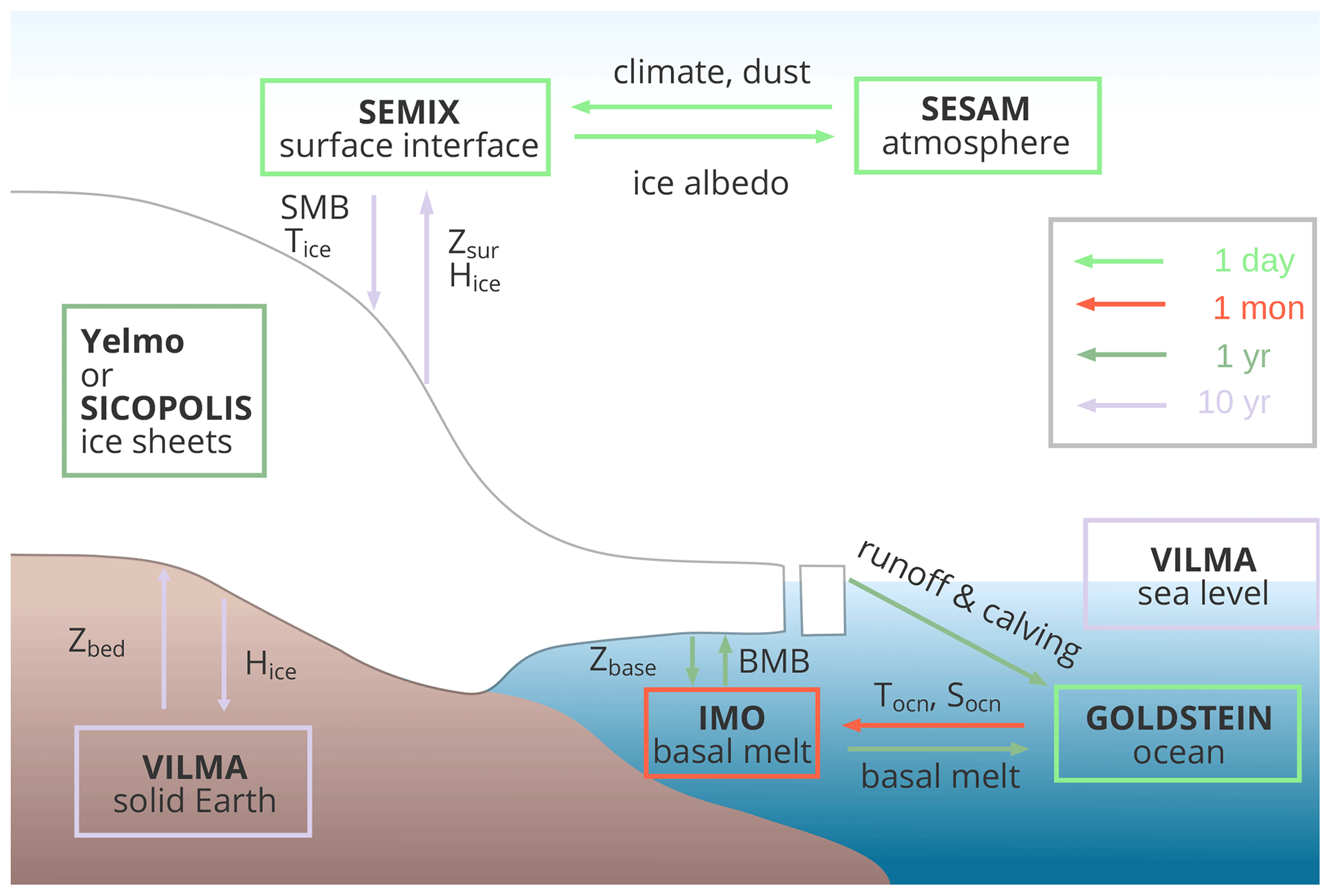
Figure 1 Schematic illustration of the coupling of the ice sheets to the other CLIMBER-X model components. The colours of the arrows indicate the coupling frequency, while the colours of the boxes represent the internal time step of the different model components. The abbreviations in the figure are as follows: SMB stands for surface mass balance, T_ice stands for 10 m firn temperature, Z_sur stands for surface elevation, H_ice stands for ice thickness, Z_bed stands for bedrock topography, Z_base stands for ice sheet base elevation, BMB stands for basal mass balance, T_ocn stands for seawater temperature, and S_ocn stands for seawater salinity.

The coupling of the ice sheet model to the other CLIMBER-X components is schematically illustrated in Fig. 1 and further details of SICOPOLIS are presented in Appendix A.

A physically based surface energy and mass balance scheme (SEMIX, Surface Energy and Mass balance Interface for CLIMBER-X) is used to interface the ice sheet model with the atmosphere. In the ice sheet modelling community it is still common to use the simple positive-degree-day (PDD) model (e.g. Braithwaite, 1984; Reeh, 1991) for the computation of surface melt. However, this simplified approach computes melt only from near-surface air temperature, with potentially important implications on the simulated response of the surface mass balance to orbital forcing and climate change (e.g. Bauer and Ganopolski, 2017; Van De Berg et al., 2011; Bougamont et al., 2007). To address some of the limitations of the PDD scheme, so-called insolation–temperature methods (ITMs) have been developed that explicitly account for absorbed surface solar radiation (Robinson et al., 2010; van den Berg et al., 2008; Pollard, 1980; Pellicciotti et al., 2005; Krebs-Kanzow et al., 2018). Recently, energy balance schemes or land surface models have also been applied to compute the surface mass balance of ice sheets (e.g. Kapsch et al., 2021; Lipscomb et al., 2013; Ackermann et al., 2020). Similarly to these models, SEMIX also explicitly resolves the surface energy balance and is largely based on the ideas in Calov et al. (2005a), but with notable modifications and improvements. The climate model fields needed by SEMIX are first bilinearly interpolated from the coarse-resolution climate model grid (5°×5°) onto the high-resolution ice sheet model grid, where SEMIX operates. Subsequently, temperature, humidity, and radiation fields are elevation corrected. We do not account for the additional orographic effect on precipitation. Such an effect is crudely accounted for by the atmospheric component of CLIMBER-X, which has a much higher resolution compared to CLIMBER-2, where a parameterization of the orographically forced precipitation was included (Calov et al., 2005a). Snow albedo depends on snow grain size and the concentration of dust in snow, while bare ice sheet albedo transitions between firn-like values, clean-ice values, and dirty-ice values depending on the age of ice and the time it has been exposed to the atmosphere. CLIMBER-X includes an interactive dust cycle (Willeit et al., 2022, 2023), and the dust concentration in snow is computed from the simulated dust deposition flux. The surface energy balance equation is then solved following a similar approach as over land and sea ice as described in Willeit and Ganopolski (2016) and Willeit et al. (2022), and the surface mass balance is finally derived accounting for snowfall, rainfall, evaporation or sublimation, melt, refreezing, and runoff. The performance of SEMIX for Greenland in the fully coupled CLIMBER-X configuration has already been presented in Höning et al. (2023). In order to compute the annual surface mass balance, SEMIX is called every 10 years over a full year with a time step of 1 d. As long as the forcing is slow enough, a higher frequency of SEMIX calls is not needed to accurately capture the climatological evolution of the surface mass balance because CLIMBER-X does not resolve weather and internal inter-annual variability. SEMIX is described in detail in Appendix B.

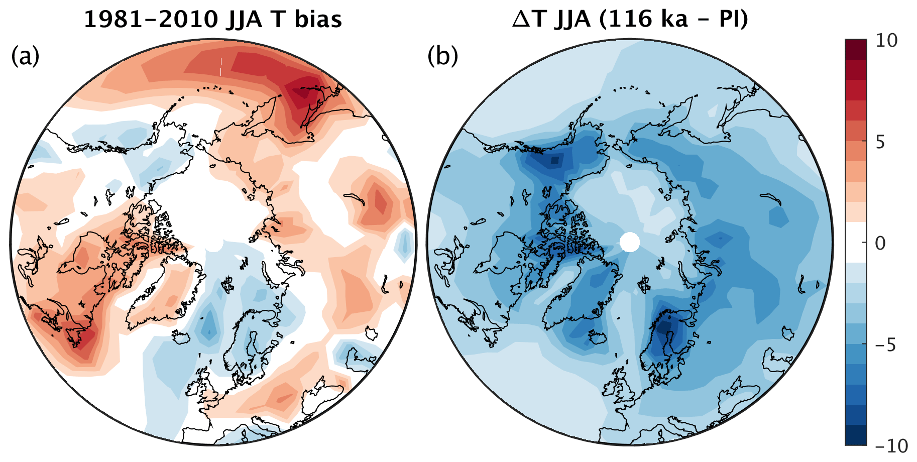
Figure 2 (a) CLIMBER-X summer (JJA) near-surface air temperature bias relative to ERA5 reanalysis (Hersbach et al., 2020) for the time period 1981–2010. (b) Difference in simulated summer (JJA) near-surface air temperature between 116 ka and pre-industrial values resulting only from the different orbital parameters.

The surface mass balance of ice sheets is largely controlled by air temperature and precipitation and relatively small climate model biases can result in large changes in simulated ice sheets (e.g. Niu et al., 2019). In accordance with Milankovitch theory, ice sheets are particularly sensitive to summer temperatures, which control snow and ice melt. Thus, even small summer temperature biases, which are common even in state-of-the-art climate models (e.g. Fan et al., 2020), can therefore preclude a realistic simulation of ice sheet growth and decay. In CLIMBER-X, present-day summer temperature biases over NH land are generally within a few degrees (Fig. 2a). However, in the area around Hudson Bay and the Labrador Peninsula, simulated summer temperatures are up to ∼ 5 °C too warm. Biases of this order of magnitude are comparable to the temperature changes induced by changing orbital configuration (Fig. 2b) and can consequently strongly affect the simulated ice sheet distribution. Therefore, similarly to Ganopolski et al. (2010), in SEMIX we implemented a temperature bias correction over northern North America as shown in Fig. B1. The bias correction is applied throughout the year as a constant offset in the computation of the surface energy balance. The reasoning behind the choice of applying summer temperature bias correction throughout the year is guided by the fact that, following Milankovitch theory, ice sheet surface mass balance is largely determined by ablation during summer, which is highly sensitive to temperature. We have actually also tested the use of bias correction applying monthly mean temperature differences, but the model results indicated absolutely negligible differences compared to using the mean summer bias. We also assume that the bias is a persistent feature of the model also under different boundary conditions and therefore apply the same bias correction at all times. Since the focus of our study is on the last glacial inception and the boundary conditions at ∼ 120 ka (just before the expected onset of ice sheet growth) are similar to pre-industrial values in terms of GHG concentrations and orbital parameters, we do not expect significant differences in temperature biases compared to the present day. The assumption on stationarity of the temperature biases is therefore, at least during the initial ice growth phase, well justified. Furthermore, since air temperature is closely related to the downwelling long-wave radiation at the surface, which affects the surface energy balance, we additionally correct the downwelling long-wave radiation using a simple quadratic relation derived from ERA5 reanalysis data. For more details, see Appendix B2.

As soon as an ice sheet gets in contact with the ocean its mass balance is also influenced by melting and freezing at the base of the floating ice shelves. At present, basal melt is important mostly for the Antarctic ice sheet, which is in extensive contact with the ocean, and for the interactions of the Greenland ice streams with the fjords. However, little is known about the role played by basal melt for ice sheets in the NH during the last glacial cycle. The basal melt is strongly influenced by the ocean circulation on the continental shelf and by the turbulent plume dynamics generated at the ice–water interface by the density difference between the fresh meltwater and the surrounding saline seawater (e.g. Jenkins, 1991). These processes can not be properly represented at the typically applied resolutions of global ocean circulation models, and several simple parameterizations have been put forward to represent the basal melt process in ice sheet models based on large-scale ambient properties of seawater and on the ice shelf base topography (Beckmann and Goosse, 2003; Holland et al., 2008; Pollard and Deconto, 2012). Simple box models have also been developed to describe the ocean circulation in the cavities below the ice shelves (Olbers and Hellmer, 2010; Reese et al., 2018; Pelle et al., 2019), but they are specifically designed to be applied to Antarctica, and an extension to the NH is not straightforward. In CLIMBER-X we have therefore implemented the simple and general basal melt parameterizations of Beckmann and Goosse (2003) and Pollard and Deconto (2012), both of which rely on the difference between the ambient ocean temperature simulated by the ocean model and the freezing point temperature of seawater at the ice shelf base. The linear model of Beckmann and Goosse (2003) has been used in the simulations presented in this work. A more general 2D plume model also including the Coriolis effect that is general enough to be applied to any ice shelf geometry has been recently developed (Lambert et al., 2022) and will be considered for a future implementation in CLIMBER-X. See Appendix C for more details on the basal melt schemes in CLIMBER-X.

The presence of ice sheets also affects the simulated freshwater fluxes into the ocean. Freshwater produced by melt occurring at the surface of the ice sheets is routed to the ocean following the steepest surface gradient, and the same runoff directions are used also to route the water originating from basal melt of grounded ice to the ocean. The freshwater flux from basal melt of floating ice and ice shelf calving is applied locally to the ocean model. Both liquid water runoff and calving fluxes are distributed uniformly over several coastal grid cells. For calving fluxes the latent heat needed to melt the ice is also accounted for in the ocean model. CLIMBER-X so far does not include an iceberg model to explicitly simulate the fate of ice originating from ice shelf calving.

The glacial isostatic adjustment (GIA), which controls regional sea level change and surface displacements, is computed by the viscoelastic solid Earth model VILMA (Klemann et al., 2008; Martinec et al., 2018; Bagge et al., 2021). In VILMA, mass conservation between ice and ocean water is considered, and the loading effect of the ice and gravity-consistent redistribution of water in the ocean is solved applying the sea level equation (Farrell and Clark, 1976) including the rotational feedback (Martinec and Hagedoorn, 2014). VILMA takes the ice sheet loading as input and computes the relative sea level (RSL) changes. The sea-level equation at the surface is solved on a Gauss–Legendre grid of 512 × 256 grid points (n128), which is consistent with the spectral resolution in spherical harmonics up to a Legendre degree or order of 170, corresponding to a wavelength of ∼ 120 km. In this study we use the 3D viscosity structure from Bagge et al. (2021), which is based on a 3D tomography model of the upper mantle seismic velocity structure that is converted into viscosity variations considering further constraints by geodynamics and lithospheric structure. In CLIMBER-X, the solid Earth dynamics determines the bedrock elevation through simulated changes in relative sea level. The relative sea level computed by VILMA is substracted as an anomaly from the reference high-resolution (≈ 10 arcmin) bedrock elevation from Schaffer et al. (2016). This is done in order to preserve the small-scale structure, which is important both for runoff routing and for surface mass balance. Surface elevation, land–sea mask, and runoff routing directions are then updated accordingly. The surface elevation is then aggregated to the coarse climate model resolution, and the land and ocean grid cell fractions on the climate model grid are then derived. The climate model in CLIMBER-X can deal with land–sea mask changes, a feature that is rather exceptional for contemporary Earth system models (e.g. Meccia and Mikolajewicz, 2018; Riddick et al., 2018). VILMA is called every 10 years, implying that the ice sheet model gets an update of the bedrock elevation field every 10 years and that the topography, the land–sea mask and the runoff directions are also updated every 10 years. Experiments using a higher coupling frequency of 1 year showed negligible differences. In a recent study coupling VILMA with the PISM ice sheet model Albrecht et al. (2023) showed a coupling time step of 100 years as being sufficient.

3 Experimental design

We first performed a transient Holocene simulation from 10 ka to present day (2000 CE) to make sure that no glacial inception is simulated at present. Since for this purpose we are mainly interested in the growth of ice sheets outside of Greenland, the Holocene simulation was performed with a prescribed present-day Greenland ice sheet. In this simulation, the model is driven by prescribed changes in the orbital configuration and atmospheric concentrations of CO₂, CH₄ and N₂O from ice core data and historical observations (Köhler et al., 2017). Note that NH summer insolation is continuously decreasing over the Holocene, although not enough to cause a glacial inception at present (Ganopolski et al., 2016). At the end of the transient Holocene simulation ice cover is consistently simulated only over parts of Baffin Island and Ellesmere Island, in the southeast of Iceland, on Svalbard, over part of Novaya Zemlya, and in a small area over the Rocky Mountains (Fig. 3), in good agreement with glacier inventories (Pfeffer et al., 2014).

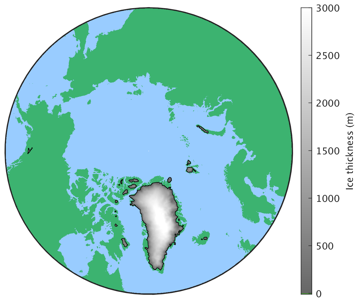
Figure 3 Present-day (2000 CE) ice sheet extent and thickness from the reference transient Holocene CLIMBER-X simulation. The Greenland ice sheet is prescribed in this experiment.

Table 1 List of last glacial inception experiments. T offset indicates the uniform and constant temperature offset added to the simulated surface air temperature in the SEMIX model when computing the surface energy and mass balance. Geo indicates whether the topography and land–ocean–ice sheet mask are updated in the simulations or not. Snow albedo offset indicates the uniform and constant offset in snow albedo applied in SEMIX.

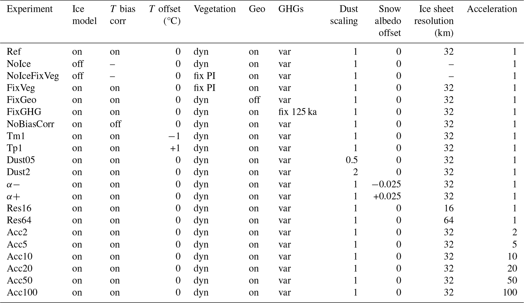
The transient last glacial inception simulations are started from the Eemian interglacial at 125 ka and run until 100 ka. This time interval is characterized first by a decrease in NH summer insolation, with a minimum reached at ∼ 116 ka followed by an increase in insolation until ∼ 105 ka (Fig. 4a). The model is driven by prescribed changes in the orbital parameters and atmospheric concentrations of CO₂, CH₄ and N₂O from ice core data (Köhler et al., 2017) (Fig. 4b). The initial conditions of the model runs correspond to the climate model in equilibrium with 125 ka boundary conditions. We therefore make the reasonable assumption that climate was in quasi-equilibrium at 125 ka. Because the Greenland ice sheet was likely not in equilibrium with climate at this time, for practical reasons we choose to start from the Greenland ice sheet prescribed from present-day observations with a uniform ice temperature of −10 °C. This is justified because Greenland is not the focus of our study and plays a negligible role in the glacial inception over the NH continents. With this general setup we performed different simulations to test the importance of different processes, namely (i) vegetation feedback, (ii) ice sheet feedback, and (iii) role of CO₂ variations, and additional experiments to explore the sensitivity of the simulated last glacial inception to (i) the temperature bias correction in SEMIX, (ii) snow albedo parameterization, (iii) ice sheet model resolution, and (iv) climate acceleration factor. The full set of experiments is listed in Table 1.

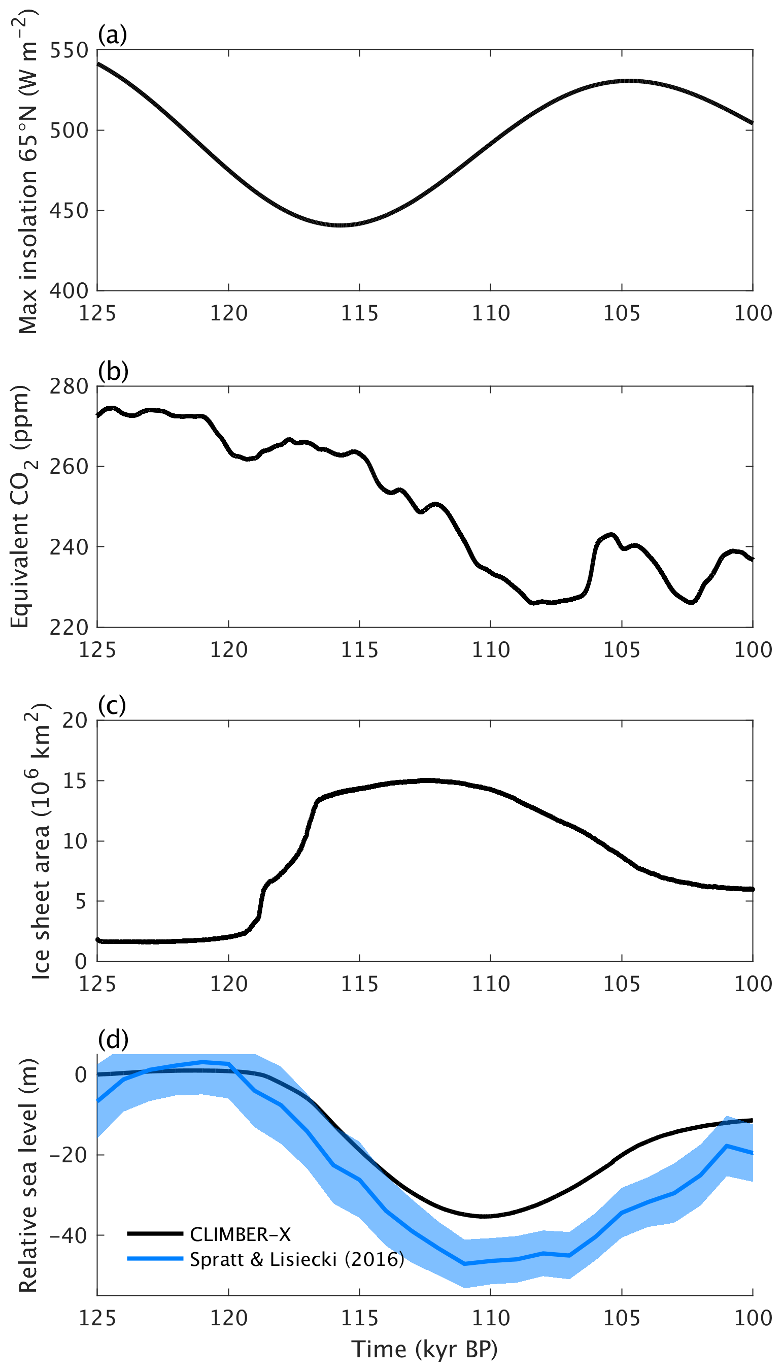
Figure 4 Transient last glacial inception simulation with reference model parameters. (a) Maximum summer insolation at 65 ° N (Laskar et al., 2004), (b) equivalent CO₂ concentration for radiation (including the radiative effect of CO₂, CH₄, and N₂O; Köhler et al., 2017). (c) Simulated ice sheet area. (d) Simulated global relative sea level change compared to reconstructions (Spratt and Lisiecki, 2016). The blue shading indicates the 1 standard deviation uncertainty range.

4 Modelling results

4.1 Reference transient simulation of the last glacial inception

In the transient simulation of the last glacial inception, until ∼ 120 ka only minor changes in ice sheet area (Fig. 4c) and sea level (Fig. 4d) are produced by the model. This is followed by a rapid increase in ice sheet area by ∼ 10 million square kilometres between ∼ 119 and ∼ 117 ka (Fig. 4c), driven by the further decrease in NH summer insolation (Fig. 4a). Afterwards, ice area stabilizes, while ice volume continues to grow and sea level drops to ∼ −35 m by ∼ 110 ka. After ∼ 110 ka both ice area and volume decrease again following an increase in summer insolation and despite a global cooling induced by a pronounced decrease in the atmospheric concentration of greenhouse gases, mainly CO₂ (Fig. 4b). There is an overall good agreement between simulated and reconstructed sea level in terms of timing, while the amplitude of the changes is somewhat underestimated (Fig. 4d). Part of this discrepancy could be related to the missing contribution from Antarctica, which is prescribed at its present-day state in our simulations and could have contributed ∼ 5 m to the sea level drop (e.g. Huybrechts, 2002; Albrecht et al., 2020).

A two-stage relation between ice sheet area and ice sheet volume in the first part of the glacial inception simulation is clearly shown in Fig. 5. Initially, a substantial increase in ice area occurs at a nearly constant ice volume, followed by a large increase in ice volume while the ice area remains almost constant. During the deglaciation phase no two-stage behaviour in the area–volume relation is found.

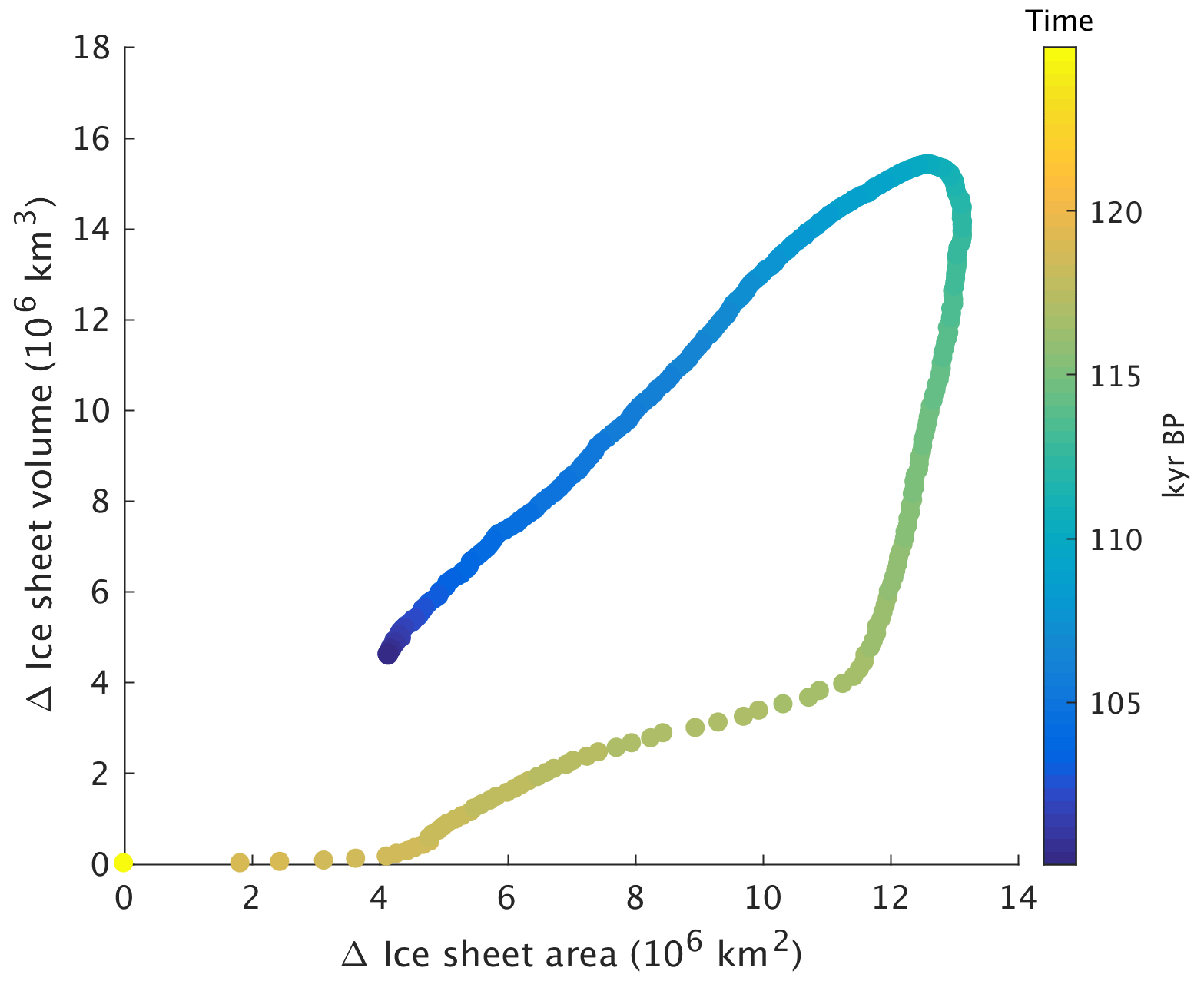
Figure 5 Relation between NH ice sheet area changes and ice sheet volume changes for the glacial inception simulation with the reference model version. Symbols indicate the area and volume every 50 years. The colour scale shows the progression of time.

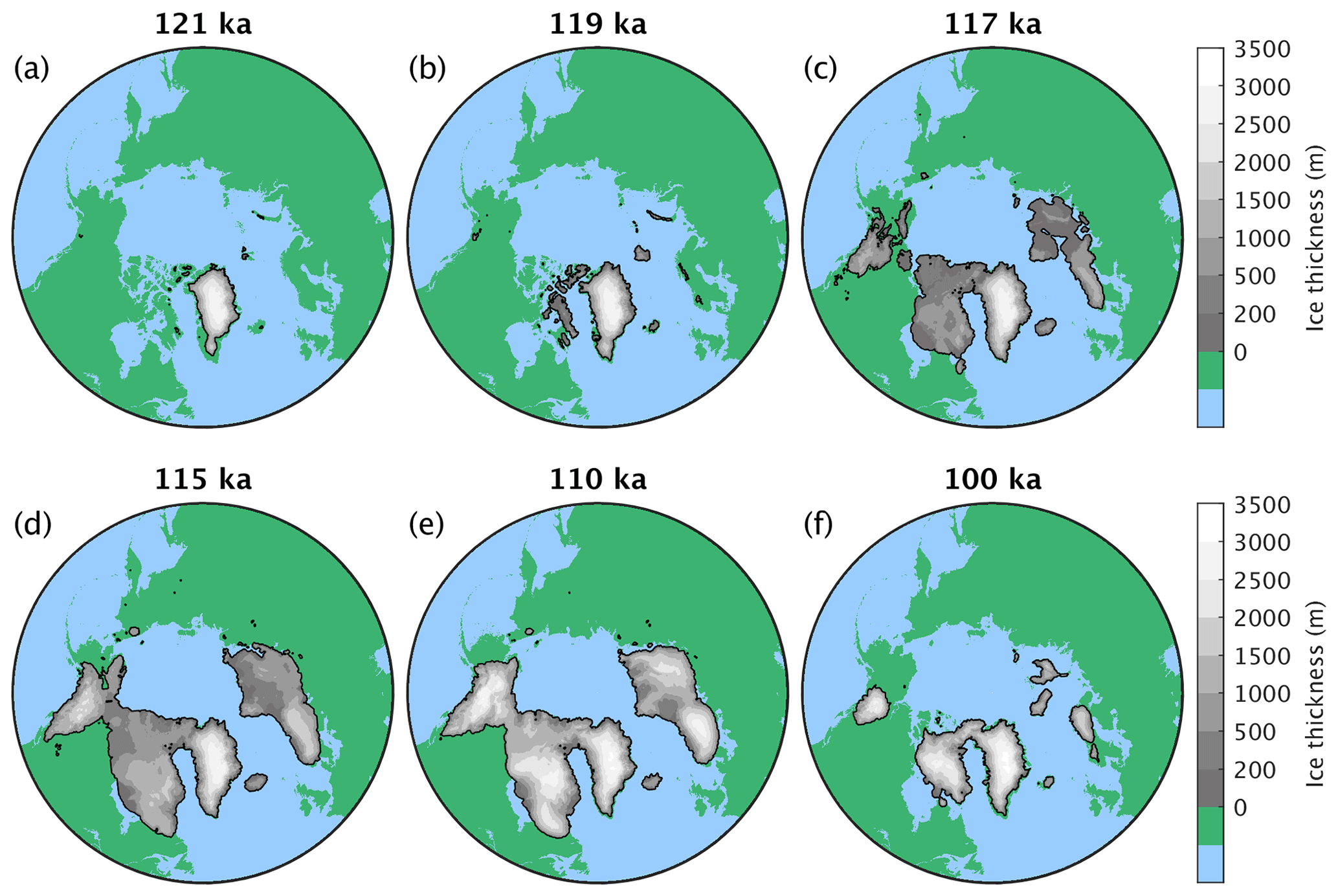
Figure 6 Ice sheet extent and thickness at different points in time for the reference last glacial inception simulation.

At 121 ka the simulated ice sheet extent is comparable to the present day but with some loss of ice in southern Greenland (Fig. 6a). The ice then starts to nucleate at high altitudes in the Arctic islands and over the mountain ranges of Scandinavia and the Ellesmere and Baffin islands (Fig. 6b) before rapidly expanding over the Canadian Arctic Archipelago and Scandinavia, mainly due to large-scale thickening of snowfields (Fig. 6c). This is in line with what has been found by Bahadory et al. (2021). Starting from the Arctic islands, ice also spreads into the Barents and Kara seas and the Cordilleran ice sheet is established (Fig. 6c). The ice then generally grows thicker and slowly expands to reach its maximum extent at ∼ 115 ka (Fig. 6d). Between 115 and 110 ka, ice sheets mainly grow thicker with little change in ice extent (Fig. 6e). Towards the end of the simulation at ∼ 100 ka, about two-thirds of the maximum “glacial” ice is melted (Fig. 6f).

The simulated ice sheet cover at 110 ka compares reasonably well with the reconstructions of Dalton et al. (2022) and Batchelor et al. (2019) for marine isotope stage (MIS) 5d (Fig. 7), also considering the relatively large associated uncertainty range (shown by the best and maximum reconstructed ice extent in Fig. 7). Models and reconstructions show a good agreement in ice sheet cover over Fennoscandia, Iceland, and Greenland. Simulated ice cover is possibly underestimated over eastern North America, particularly over the Labrador region, although reconstructions are highly uncertain over this region. A Cordilleran ice sheet is formed in the model, while Alaska remains largely ice free. Contrary to what is indicated by the reconstructions mentioned above, the Cordilleran and Laurentide ice sheets merge in the model simulation. Little ice cover is simulated by the model over eastern Siberia, where reconstructions suggest the presence of small ice caps covering the mountain ranges.

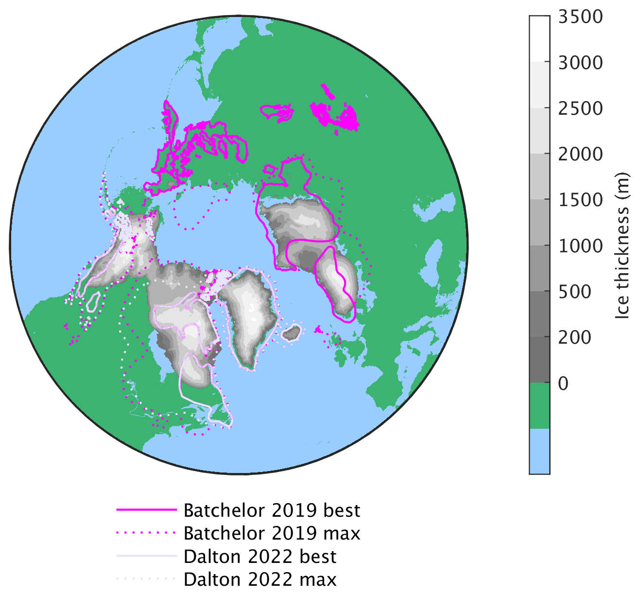
Figure 7 Simulated ice sheet extent at 110 ka (MIS5d) compared to the best and maximum extent reconstructions from Dalton et al. (2022) and Batchelor et al. (2019).

The relative sea level represents the geoid height change relative to the displaced Earth surface. Its signature at 110 ka, shown in Fig. 8, mainly represents the sum of the viscoelastic subsidence due to the loading of the ice sheet as geoid changes due to gravitational changes and due to the mass conservation between ice and ocean. Accordingly, the RSL rise in the loaded regions is dominated by the subsidence of the Earth surface due to the viscoelastic response of the solid Earth, whereas the drop over the oceans reflects the mass conservation between ice and ocean, meaning the water equivalent of the ice sheet mass. Furthermore, the ice sheets are surrounded by regions of lower RSL due the forebulge of the flexed elastic lithosphere. The bedrock deformation and depression is largest at the centres of the ice sheets, corresponding to a RSL that is up to 500 m higher than pre-industrial values, while the far-field RSL is ∼ 35 m lower than pre-industrial values (Fig. 8). Alaska shows the highest RSL values, which can be attributed to the low viscosity structure of the solid Earth in this region allowing a faster rebound in comparison to the cratonic areas of NE Canada and Scandinavia (see viscosity structure in Fig. D1 in Appendix D).

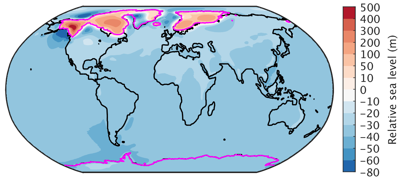
Figure 8 Simulated relative sea level changes relative to pre-industrial values at 110 ka. The magenta lines indicate the ice sheet extent.

In terms of changes in climate, from 125 to 110 ka the model shows a pronounced summer cooling at middle to high northern latitudes (Fig. 9c) as a direct response to the decrease in summer insolation (Fig. 9a), amplified by a strong albedo increase (Fig. 9b), which is driven by a combination of expanding sea ice, a southward shift of the treeline (Fig. 10), and the establishment of land ice. Going from 121 to 115 ka, summer temperatures undergo a substantial cooling over most of the NH, particularly over land (Fig. 11).

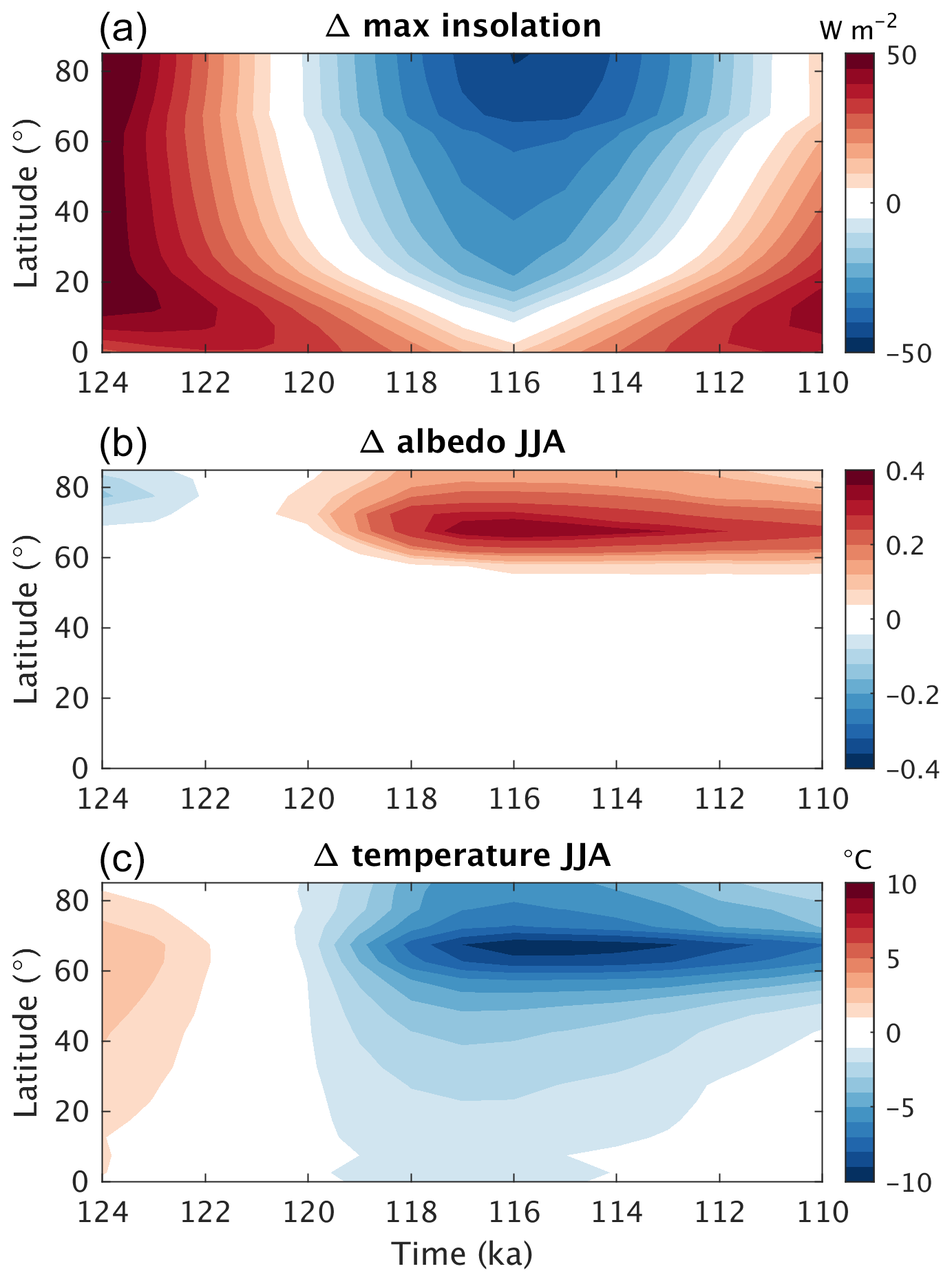
Figure 9 Northern Hemisphere zonal mean differences in (a) maximum summer insolation, (b) summer (JJA) surface albedo, and (c) summer (JJA) surface air temperature as a function of time for the reference glacial inception simulation relative to the pre-industrial values.

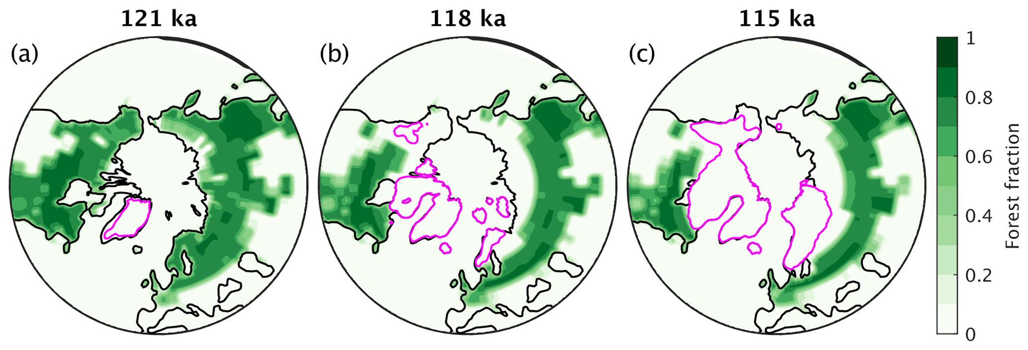
Figure 10 Forest fraction at different points in time simulated by the model in the reference experiment. The magenta lines indicate the ice sheet extent.

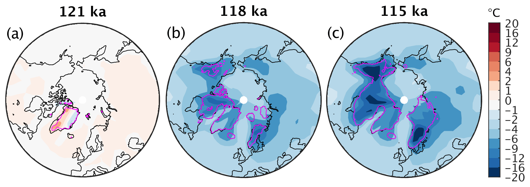
Figure 11 Summer (JJA) temperature difference relative to the pre-industrial values at different times in the reference glacial inception simulations. Note the non-linear colour scale.

4.2 Role of vegetation, ice sheet, and carbon cycle feedbacks

The effect of the vegetation feedback on the expansion of ice sheets during glacial inception can be quantified by running a glacial inception simulation with vegetation prescribed at its pre-industrial state. Practically, fixed vegetation in our simulation means that the plant functional type fractions are not allowed to change and that the maximum leaf area index is fixed. However, for deciduous plants, the seasonality of the phenology will still be affected by the changing climatic conditions. The vegetation feedback plays a crucial role for glacial inception in our simulations. This is clearly illustrated by the much smaller increase in ice sheet area and volume in simulations where vegetation is prescribed at its equilibrium pre-industrial state, compared to the reference glacial inception simulation with interactive vegetation (Fig. 12).

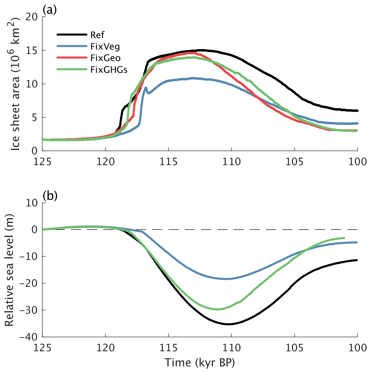
Figure 12 (a) Ice sheet area and (b) relative sea level changes for model simulations with fixed vegetation (blue), fixed present-day topography and land–ocean–ice sheet mask (red), and fixed 125 ka greenhouse gas concentrations (green) compared to the reference simulation (black).

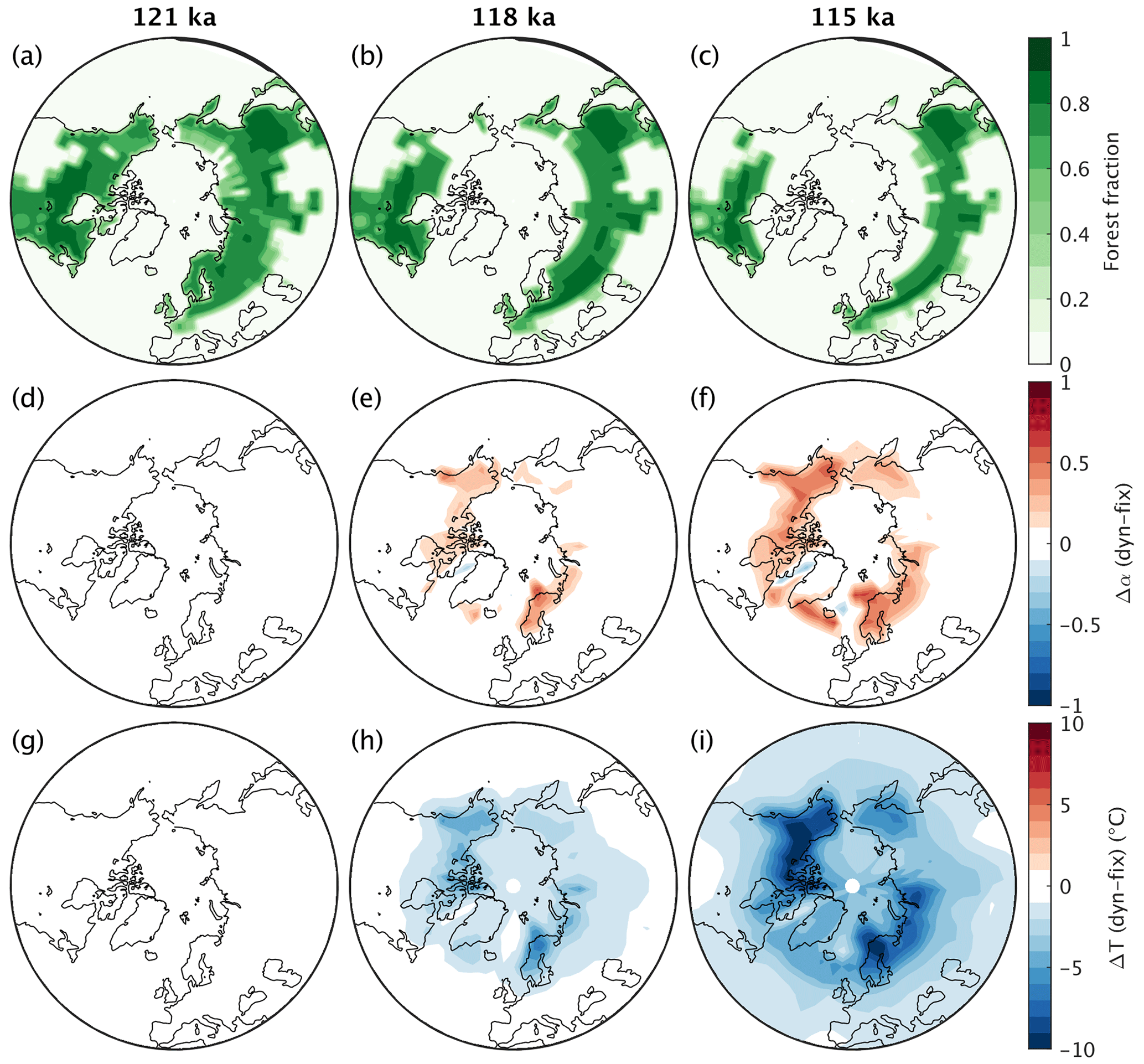
Figure 13 (a–c) Simulated forest fraction at different times during the glacial inception simulation with dynamic vegetation but prescribed present-day ice sheets (simulation NoIce). Differences in (d–f) surface albedo and (g–i) surface air temperature in late spring–early summer (May–June–July) between simulations with prescribed present-day ice sheets and dynamic (NoIce) and fixed (NoIceFixVeg) vegetation at different times.

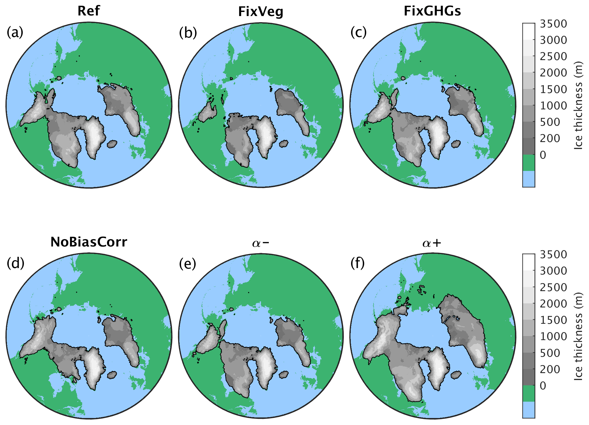
Figure 14 Simulated ice sheet extent and thickness at 115 ka for different experiments: (a) reference, (b) fixed pre-industrial vegetation, (c) fixed 125 ka GHGs concentrations, (d) no temperature bias correction over North America, (e) reduced snow albedo, and (f) increased snow albedo.

The effect of dynamic vegetation on climate can be isolated from two simulations, one with prescribed vegetation and one with dynamic vegetation, both without interactive ice sheets. The strong vegetation feedback is explained by a pronounced southward shift of the northern boreal treeline as a response to the gradual decrease in summer insolation at high northern latitudes during glacial inception (Fig. 13a–c). The expansion of tundra at the expense of taiga results in a substantial increase in surface albedo during the snow-covered season (Fig. 13d–f) with a particularly strong associated cooling in spring, which also extends into the summer months (Fig. 13g–i). This explains why the ice extent in the simulation with prescribed vegetation is generally reduced compared to the interactive vegetation case (Fig. 14a and b).

Our results on the important role played by the vegetation feedback for the initiation of NH glaciation are consistent with a number of previous studies that have shown that the vegetation response during the last glacial inception amplifies the orbitally induced summer cooling in high northern latitudes (Harvey, 1989; De Noblet et al., 1996; Meissner et al., 2003; Crucifix and Loutre, 2002; Yoshimori et al., 2002), thus favouring the growth of ice sheets (Kageyama et al., 2004; Calov et al., 2005b; Mysak, 2008; Kubatzki et al., 2006).

The effect of ice sheets on glacial inception can be quantified with a simulation in which the land–ocean–ice sheet mask and the topography are prescribed at their pre-industrial state. This is equivalent to disabling the back-coupling of the ice sheets to the climate model and therefore suppressing the ice sheet feedback on climate. The model results indicate that this ice sheet feedback plays only a minor role during the ice growth phase until ∼ 115 ka (Fig. 12). This is explained by the ice expansion being driven by a rapid increase of perennially snow-covered area rather than by a slow lateral expansion of ice sheets. However, the higher albedo of ice compared to ice-free land plays an important role in slowing down the ice sheet melt during the ice retreat phase following the rising summer insolation after 115 ka (Fig. 12).

The role of the CO₂ variations during glacial inception can be estimated from a simulation where the atmospheric concentrations of the greenhouse gases are kept constant at their 125 ka values. Since the GHG concentrations show only small variations until ∼ 115 ka (Fig. 4b), it is not surprising that the GHG forcing plays only a minor role during the first phase of glacial inception (Fig. 12). Hence, the simulated ice sheets in the experiment with prescribed constant GHGs are very similar to those in the reference simulation at 115 ka (Fig. 14a and c). However, the decrease in the equivalent CO₂ concentration after ∼ 115 ka is important for slowing down the ice sheet melt and limit deglaciation (Fig. 12).

Figure 15 Simulated (a) ice sheet area and (b) relative sea level for different uniform temperature offsets in SEMIX (experiments Tp1 and Tm1 in Table 1) and for the simulation without temperature bias correction (NoBiasCorr).

4.3 Sensitivity to climate model biases

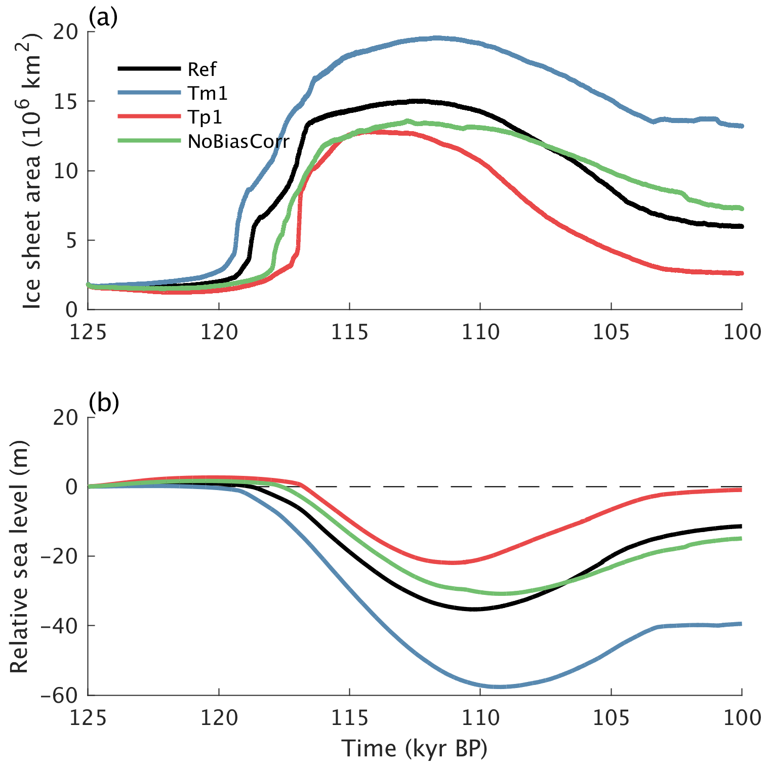
It is known that ice sheets can be highly sensitive to relatively small temperature changes. For instance, it has been shown that the bifurcation point for the complete melting of the Greenland ice sheet could be at only a few degrees above pre-industrial values (Robinson et al., 2012; Höning et al., 2023). We therefore decided to apply different uniform temperature offsets in the surface energy and mass balance model and use these for sensitivity tests. This is justified because the global mean surface air temperature is (i) quite uncertain and (ii) different state-of-the-art climate models produce very different global mean temperatures (Bock et al., 2020). Our simulations show that the last glacial inception is sensitive to relatively small temperature perturbations in the surface mass balance model (Fig. 15). In particular, the difference in simulated sea level decrease between the experiment with a uniform cooling of 1 °C and the experiment with a uniform warming of 1 °C in SEMIX is ∼ 35 m (Fig. 15).

Without the temperature correction over North America (Fig. B1), the simulated ice sheet distribution over this continent is shifted from the east to the west, as expected (Fig. 14a,d). Little ice is simulated in the area around the Hudson Bay, while ice extends further in the northwest. A similar east–west displacement of the ice distribution has also been found in other models that share temperature biases similar to the CLIMBER-X ones over North America (e.g. Bahadory et al., 2021).

4.4 Sensitivity to snow albedo parameterization

The albedo of snow is a function of snow grain size, with smaller grain sizes resulting in higher albedo (e.g. Warren and Wiscombe, 1980a; Gardner and Sharp, 2010). Fresh dry snow has a generally small grain size, but the grain size tends to increase as the snow undergoes metamorphism processes and in particular as melting occurs. Snow albedo is also affected by the presence of light-absorbing impurities, such as mineral dust or soot particles (e.g. Dang et al., 2015; Warren and Wiscombe, 1980b). Since the albedo of snow is generally high, small relative changes in snow albedo will result in large relative changes in co-albedo, which is the relevant quantity determining the amount of absorbed solar radiation at the surface. It is therefore expected that uncertainties in the parameterization of the albedo of snow will result in substantial differences in the surface energy and mass balance (e.g. Willeit and Ganopolski, 2018). To explore this we performed simulations in which we added a constant offset of ± 0.025 to the albedo of snow and experiments with half and double the dust deposition rate in SEMIX. These perturbations to the snow albedo result in a simulated sea level decrease during MIS5d that varies by more than 40 m (Fig. 16). This is remarkable considering that the snow albedo changes introduced are of the order of only a few percent. In terms of spatial pattern, the simulated ice sheet is more extended and twice as large by volume if the snow albedo is higher and less extended if the snow albedo is lower than in the reference run (Fig. 14e and f).

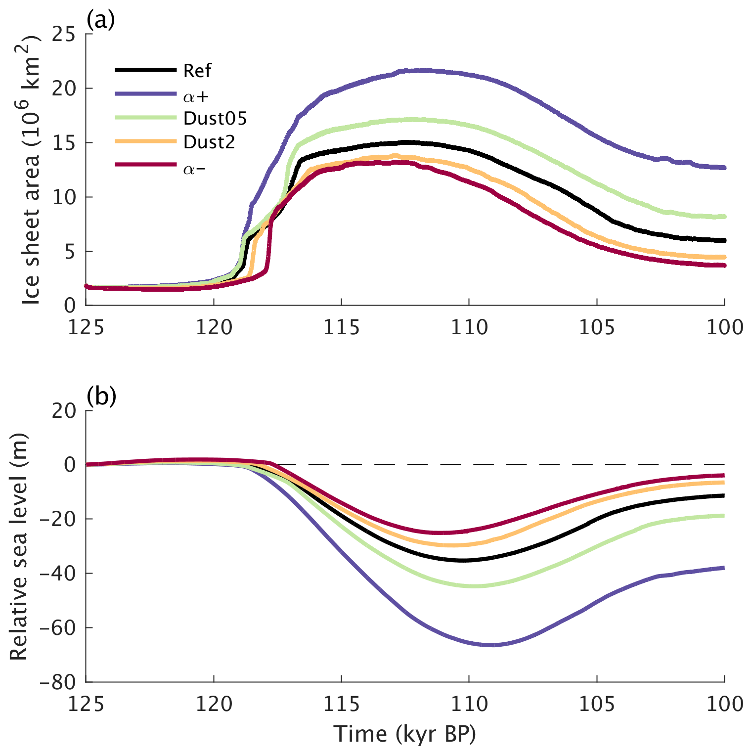
Figure 16 (a) Ice sheet area and (b) relative sea level changes for model simulations with scaled dust deposition fields and offsets in snow albedo.

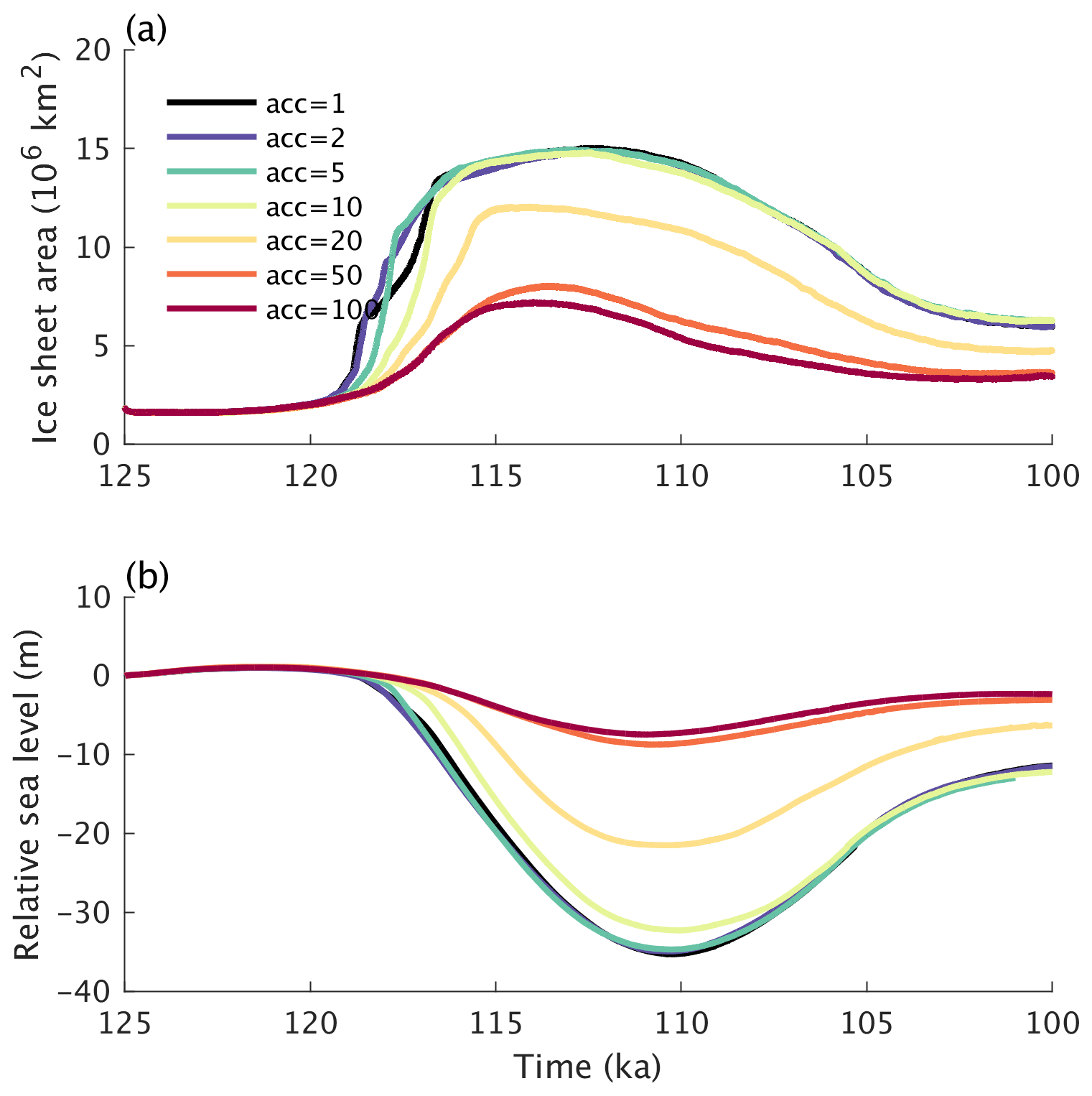
Figure 17 Simulated (a) ice sheet area and (b) relative sea level when different climate model acceleration factors are applied.

4.5 Sensitivity to climate model acceleration

Several efforts are ongoing to simulate the last glacial cycle with state-of-the-art Earth system models based on general circulation models (e.g. Latif et al., 2016). Computational time is a strong constraint for these models and acceleration techniques (e.g. Lorenz and Lohmann, 2004) are one possible way to alleviate this problem. These are based on the fact that typical timescales of the atmosphere, ocean, and vegetation are much shorter than orbital timescales. This allows for the to artificial acceleration of the external forcings, in this case orbital parameters and GHGs concentration, which, considering that the atmosphere and ocean are also the most computationally expensive parts of an Earth system model, results in an effective speed-up of the model. The ice sheet model cannot be accelerated in the same way. However, this is not problematic because ice sheet models are comparatively less computationally demanding.

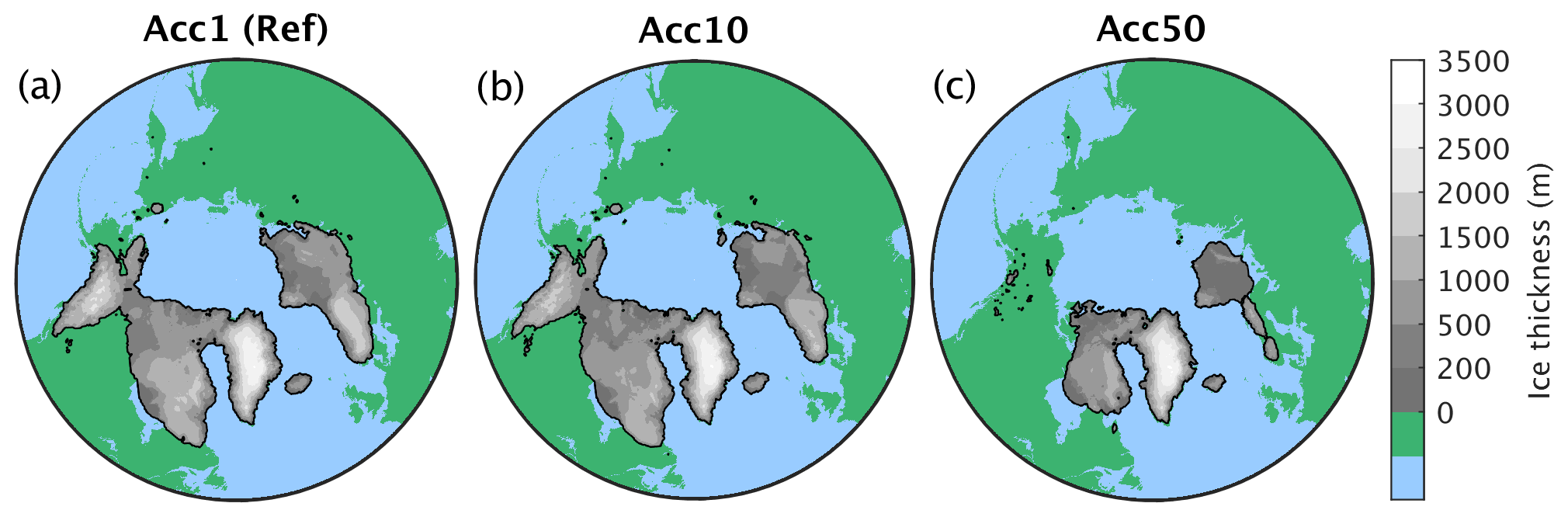
Figure 18 Simulated ice sheet extent and thickness at 115 ka for simulations with different climate acceleration factors: (a) reference run without climate acceleration, (b) acceleration factor of 10, and (c) acceleration factor of 50.

To assess the applicability of the acceleration technique, we perform additionally several experiments with different acceleration rates to explore how sensitive the ice sheet evolution during glacial inception is to the applied acceleration factor. Our results show only a relatively weak sensitivity of the ice sheet evolution to climate acceleration for acceleration factors up to ∼ 10 (Fig. 17), confirming earlier results from the CLIMBER-2 model (Calov et al., 2009; Ganopolski et al., 2010). Much larger accelerations factors do not allow for a proper representation of the positive climate feedbacks at work during glacial inception, resulting in reduced simulated ice extent and volume (Fig. 18).

4.6 Sensitivity to ice sheet model resolution

We also tested the dependence of the simulated glacial inception on the resolution of the ice sheet model. A higher-resolution ice sheet model will result in a better preservation of the fine-scale topographic structure, and since the surface mass balance is strongly dependent on surface elevation, it is expected that better resolving mountain peaks would facilitate the formation of ice caps. It is unclear, however, whether this would facilitate the formation of large-scale ice sheets or not, also because better resolving mountains also implies that deep valleys are better resolved, which would inhibit the spreading of ice from isolated ice caps to larger-scale ice sheets.

Our simulations show only a weak dependence of the model results on the resolution of the ice sheet model in the tested range between 16 and 64 km (Fig. 19). However, some local ice caps that are formed with a high-resolution ice sheet model are not resolved when the resolution is decreased (Fig. 20).

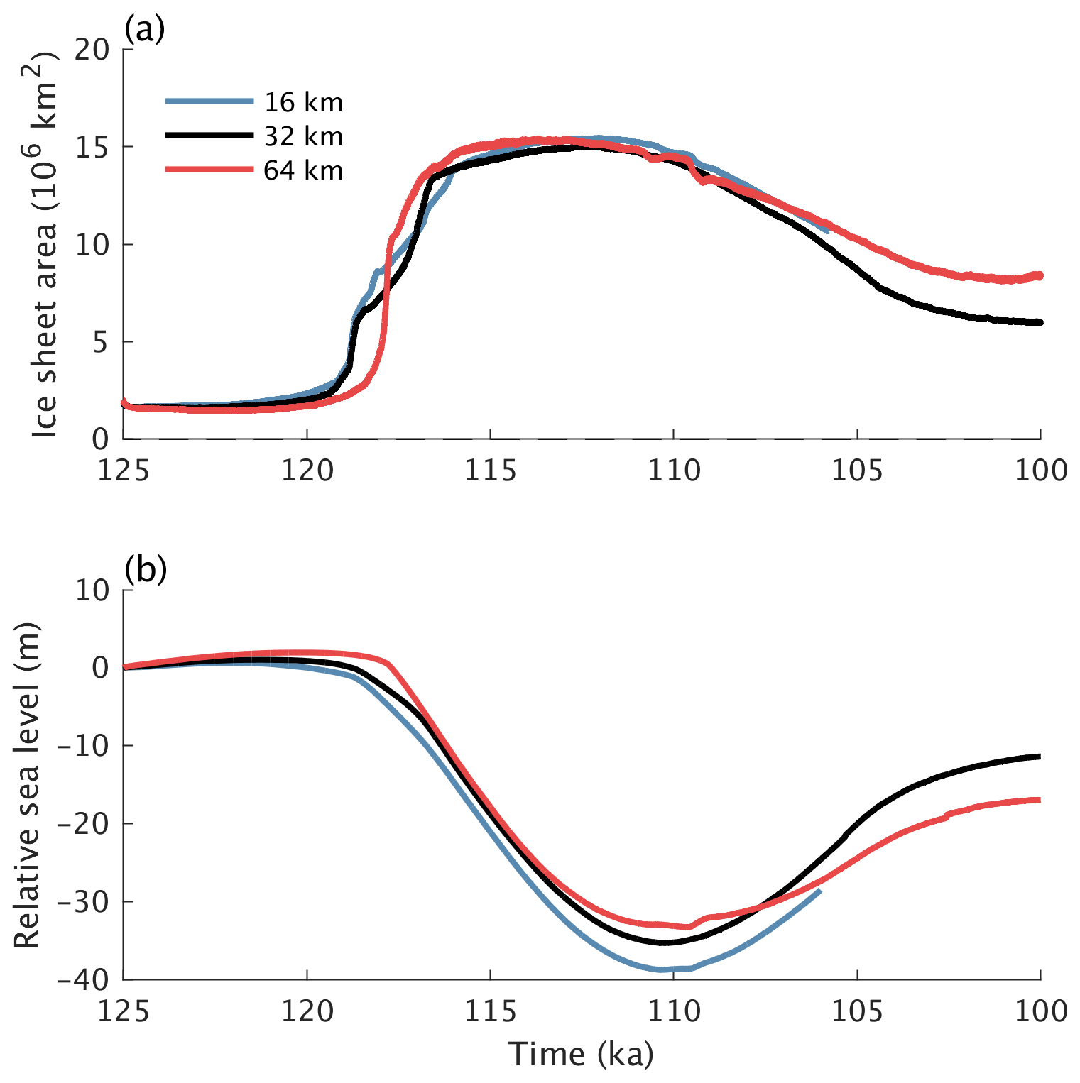
Figure 19 Simulated (a) ice sheet area and (b) relative sea level for different resolutions of the ice sheet model.

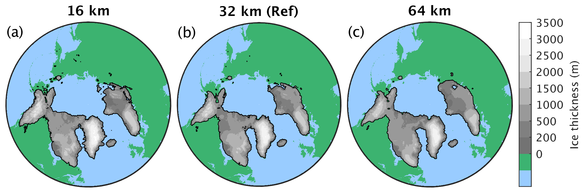
Figure 20 Simulated ice sheet extent and thickness at 115 ka for simulations with different horizontal resolutions of the ice sheet model: (a) 16 km, (b) 32 km (Ref), and (c) 64 km.

5 Discussion and conclusions

We have presented the results of a set of transient simulations of the last glacial inception with the CLIMBER-X Earth system model, which includes an ice sheet model and a model for the solid Earth response to changes in ice sheet loading. This paper also describes the ice sheet coupling with the atmosphere and ocean, which will serve as a reference for future studies using the model with interactive ice sheets.

We have shown that, as a response to the decreasing summer insolation at high northern latitudes, the model simulates a rapid expansion of ice sheets over northern North America and Scandinavia between ∼ 120 and ∼ 116 ka, which is driven mainly by large-scale snowfield thickening. This result is fully consistent with the concept of glacial inception as a bifurcation in the climate system caused by a strong albedo feedback (Calov et al., 2005a). The rapid expansion of the ice sheet area was followed by ice volume growth that corresponds to a global sea level drop of nearly 40 m at 110 ka, which is in reasonable agreement with paleoclimate reconstructions. Compared to the CLIMBER-2 results from Calov et al. (2005a), as expected the CLIMBER-X model results are in better agreement with available paleoclimate reconstructions in terms of simulated ice volume and spatial distribution of ice sheets. The abrupt increase of the North American ice sheet extent simulated in CLIMBER-X is nearly half that shown in Calov et al. (2005a), and this increase happens in two steps. Less ice is formed in eastern Siberia and Alaska in CLIMBER-X than in CLIMBER-2. At the same time, despite substantial differences in model formulations and spatial resolution, the results of the simulations with CLIMBER-X confirm the main findings presented in Calov et al. (2005a, b). The abrupt increase in the North American ice sheet area occurs in CLIMBER-X approximately at the same time and in the same area as in Calov et al. (2005a) and through the same mechanisms. Our results confirm the critically important role of vegetation feedback demonstrated in Calov et al. (2005b). The albedo feedback associated with an increase in snow-covered area, sea ice extent, and the southward retreat of the boreal forest plays a crucial role in the rapid ice area expansion in our simulations. The vegetation feedback alone increases the maximum simulated ice sheet area by 50 %.

Our new modelling results show a strong sensitivity of simulated ice sheet evolution to the parameterization of clean snow albedo and to the impact of impurities on snow albedo. The ice sheet feedback and the variations in GHGs concentrations are of minor importance during the ice growth phase associated with decreasing summer insolation prior to ∼ 115 ka but are fundamental in maintaining the system in a glacial state during the subsequent period of increase in summer insolation, resulting in an only partial deglaciation.

The results of model simulations demonstrate that the reduction of climate biases (too high summer air temperatures over eastern North America) leads to significant improvements in the simulated spatial extent of the North American ice sheet, as also shown by Ganopolski et al. (2010).

The model results are not very sensitive to climate acceleration up to a factor ∼ 10, confirming earlier findings by Calov et al. (2009) and Ganopolski et al. (2010). Assuming that this finding also holds for more complex Earth system models, a climate acceleration factor of 10 would allow these models to run transient glacial inception simulations in a reasonable time using less computational resources. The resolution of the ice sheet model only marginally affects the model results, at least in the tested range between 16 and 64 km. This is because a large-scale ice expansion over relatively flat terrain is the dominant mechanism leading to glacial inception in our model, while ice caps, which can be captured only if the topography is highly resolved, have only a very localized effect and are therefore not of fundamental importance.

The glacial inception simulations presented here are a first step towards simulating the full last glacial cycle with CLIMBER-X.

Appendix A: SICOPOLIS ice sheet model

For the inclusion into CLIMBER-X, the original SICOPOLIS code has been restructured and organized into Fortran 90-derived types to allow running several instances of the model at the same time, one for each ice sheet domain. Although in the present study we employ a single ice sheet domain for the NH, CLIMBER-X can be set up to run with an arbitrary number of ice sheet model domains, with potentially different resolutions, simply by specifying a list of domain names in a namelist.

As already mentioned above, SICOPOLIS is based on the shallow ice approximation for grounded ice, the shallow shelf approximation for floating ice, and hybrid shallow-ice–shelfy-stream dynamics for ice streams (Bernales et al., 2017), and the enthalpy method of Greve and Blatter (2016) is used as thermodynamics solver.

In this study we use a Weertman-type sliding law to relate basal drag (τ_b) to basal velocity (u_b):

$$\begin{array}{}\text{(A1)}& {\mathit{\tau }}_{\mathrm{b}}={\displaystyle \frac{\mathrm{1}}{c_{\mathrm{s}}^{\mathrm{1}/p}}}{N}^{q/p}{u}_{\mathrm{b}}^{\mathrm{1}/p},\end{array}$$

with p=3 and q=2. N is the reduced basal pressure computed as the difference between the ice overburden pressure and the water pressure if the base of the ice sheet is below sea level:

$$\begin{array}{}\text{(A2)}& N=P_{\mathrm{i}}-P_{\mathrm{w}}={\mathit{\rho }}_{\mathrm{i}}g{h}_{\mathrm{i}}-{\mathit{\rho }}_{\mathrm{w}}gmax(\mathrm{0},z_{\text{bed}}),\end{array}$$

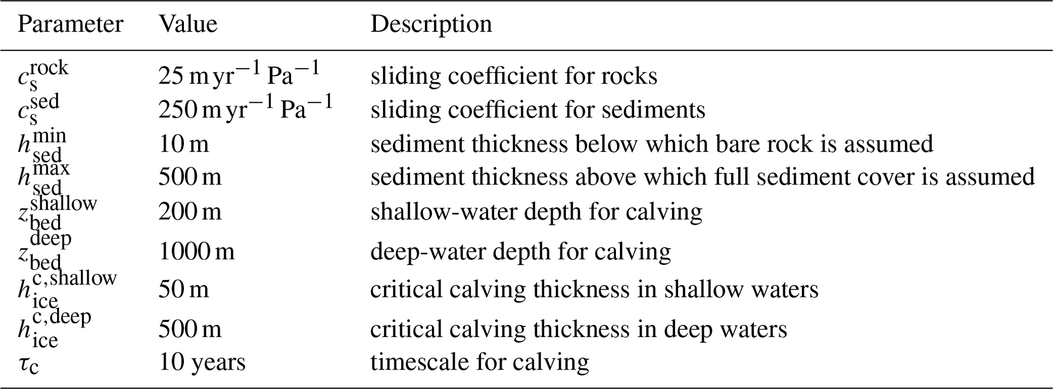
where ρ_i and ρ_w are the ice and water densities, g is the acceleration due to gravity, h_i is ice thickness, and z_bed is the bedrock depth below sea level. The c_s sliding parameter depends on the assumed sediment fraction in each grid cell:

$$\begin{array}{}\text{(A3)}& c_{\mathrm{s}}=(\mathrm{1}-f_{\text{sed}})c_{\mathrm{s}}^{\text{rock}}+f_{\text{sed}}{c}_{\mathrm{s}}^{\text{sed}}.\end{array}$$

The sediment fraction is taken to be a linear function of sediment thickness between two critical values $h_{\text{sed}}^{\text{min}}$ and $h_{\text{sed}}^{\text{max}}$:

$$\begin{array}{}\text{(A4)}& f_{\text{sed}}={\displaystyle \frac{h_{\text{sed}}-h_{\text{sed}}^{\text{min}}}{h_{\text{sed}}^{\text{max}}-h_{\text{sed}}^{\text{min}}}},\end{array}$$

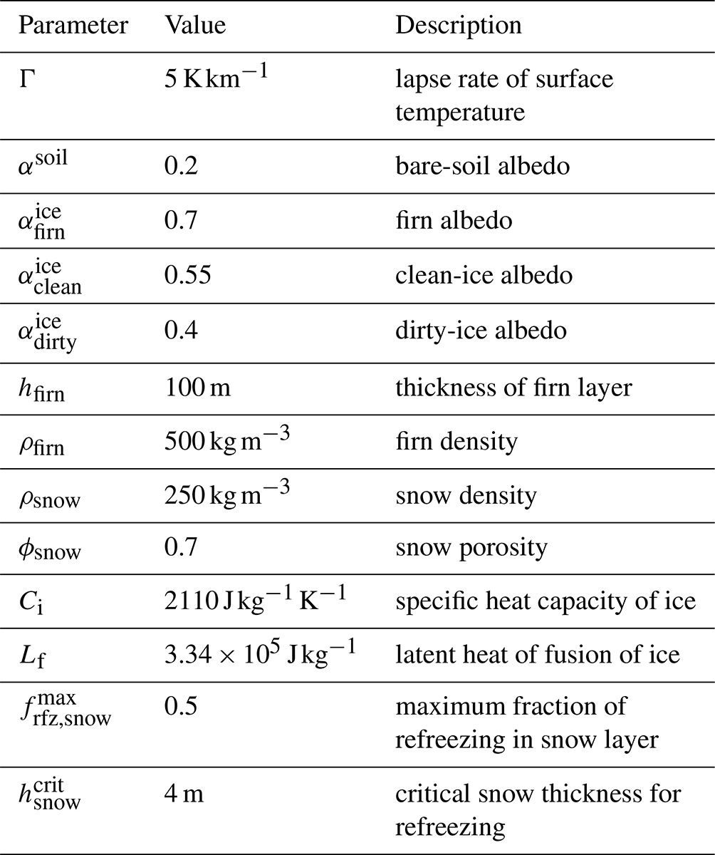
where f_sed is computed based on sediment thickness data from Laske et al. (2013) and is shown in Fig. A1. The value for bedrock is set to $c_{\mathrm{s}}^{\text{rock}}$ = 25 $\mathrm{m}{\mathrm{yr}}^{-\mathrm{1}}{\mathrm{Pa}}^{-\mathrm{1}}$ following the tuning for the Greenland ice sheet in Calov et al. (2018), while the value over thick sediments is simply taken as 10 times this value, i.e. $c_{\mathrm{s}}^{\text{sed}}$ = 250 $\mathrm{m}{\mathrm{yr}}^{-\mathrm{1}}{\mathrm{Pa}}^{-\mathrm{1}}$.

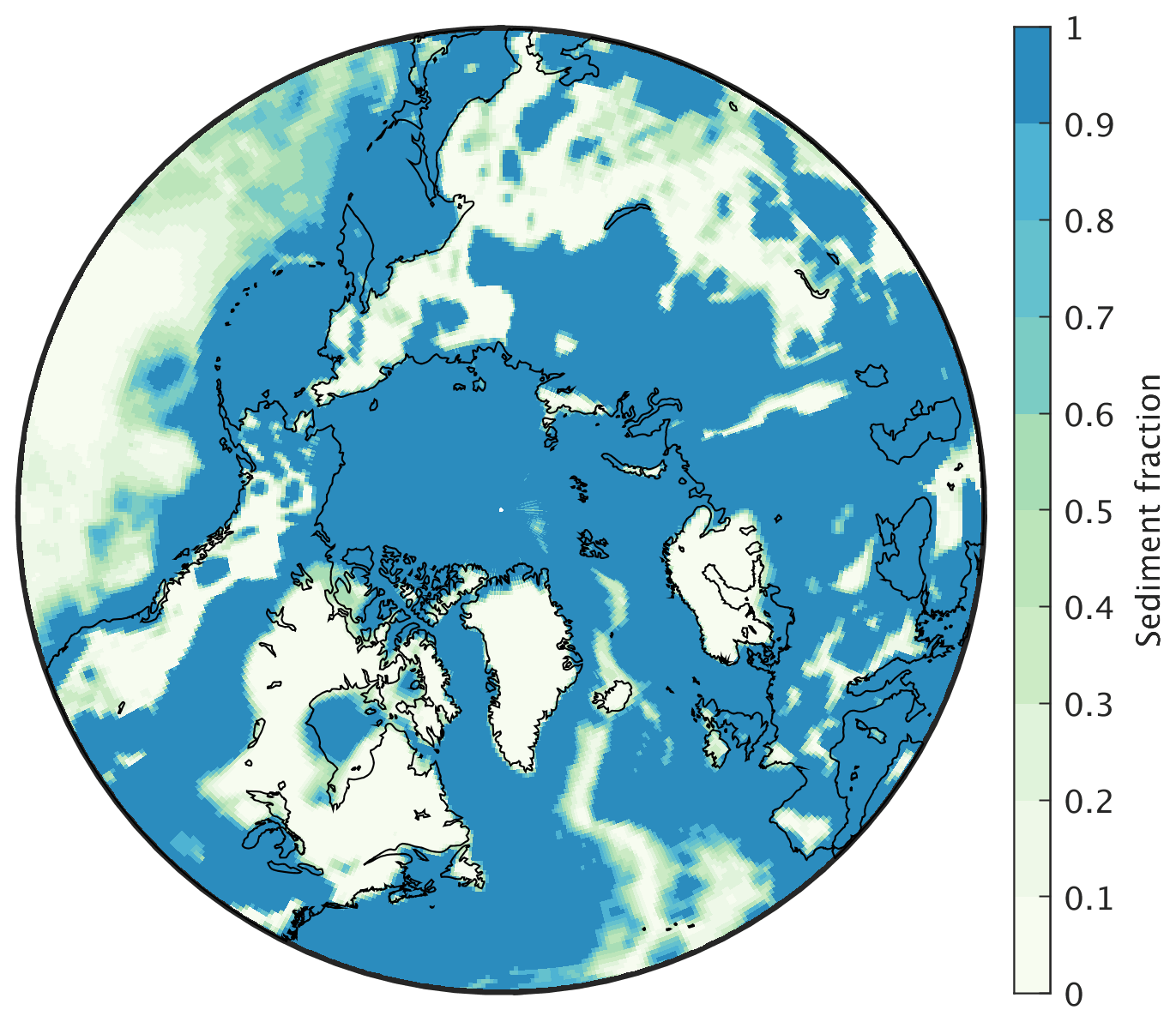
Figure A1 Sediment fraction used in the computation of the basal sliding coefficient c_s.

A broader investigation of the sliding law will be performed in forthcoming papers discussing the simulation of glacial termination, when the sliding is expected to be more important.

Iceberg calving at the marine-terminating ice front is parameterized using a simple thickness-based threshold method in which the calving rate is computed as follows:

$$\begin{array}{}\text{(A5)}& C={\displaystyle \frac{h_{\text{ice}}^{\mathrm{c}}-h_{\text{ice}}}{{\mathit{\tau }}_{\mathrm{c}}}}.\end{array}$$

Table A1 List of SICOPOLIS model parameters.

It is applied only where the ice thickness, h_ice, is lower than the critical thickness for calving, $h_{\text{ice}}^{\mathrm{c}}$, also in all neighbouring ice points. The critical thickness for calving varies spatially and increases linearly with the depth of bedrock:

$$\begin{array}{}\text{(A6)}& h_{\text{ice}}^{\mathrm{c}}=h_{\text{ice}}^{\mathrm{c},\text{deep}}+\left(z_{\text{bed}}^{\text{fil}}-z_{\text{bed}}^{\text{deep}}\right)\cdot {\displaystyle \frac{h_{\text{ice}}^{\mathrm{c},\text{deep}}-h_{\text{ice}}^{\mathrm{c},\text{shallow}}}{z_{\text{bed}}^{\text{deep}}-z_{\text{bed}}^{\text{shallow}}}},\end{array}$$

where $z_{\text{bed}}^{\text{fil}}$ is the bedrock elevation filtered with a Gaussian filter with a 100 km radius and $z_{\text{bed}}^{\text{shallow}}$, $z_{\text{bed}}^{\text{deep}}$, $h_{\text{ice}}^{\mathrm{c},\text{shallow}}$, and $h_{\text{ice}}^{\mathrm{c},\text{deep}}$ are model parameters (Table A1). Although this is only a very crude representation, it is arguably more reasonable than assuming a uniform threshold that does not account for the different ocean dynamics in the narrow channels of the Canadian Arctic Archipelago and the deep open ocean. Lower values of $h_{\text{ice}}^{\mathrm{c}}$ allow for a more rapid expansion of floating ice shelves, thereby also affecting the rate of shelf ice spreading. However, since floating ice is usually thin, this has only a minor impact on the simulated ice volume during glacial inception.

The global geothermal heat flux product of Lucazeau (2019), substituted with data from Colgan et al. (2022) over Greenland, is applied as bottom boundary condition for the bedrock temperature equation at a depth of 2 km below the land surface in SICOPOLIS.

For all simulations presented in this study we used an annual time step for the thermodynamic part and a half-yearly time step for the dynamics.

Appendix B: SEMIX surface energy and mass balance interface

SEMIX is an adaptation of the surface energy and mass balance interface (SEMI) (Calov et al., 2005a) to CLIMBER-X. Its purpose is to determine the surface boundary conditions, namely surface mass balance and surface ice temperature, for the ice sheet model. In order to do that SEMIX has to bridge the gap in resolution between the climate model and the ice sheet model, which is achieved through a downscaling of the climate variables (Appendix B1). The surface energy and mass balance equations are then solved on the high-resolution ice sheet grid as outlined in Appendix B3. Since multiple ice sheet domains are allowed in CLIMBER-X, similar to the ice sheet model SEMIX can also run in several separate instances according to the defined ice sheet domains. SEMIX is called every 10 years over a full year with a time step of 1 d.

B1 Downscaling of climate variables

SEMIX is driven by climate fields computed by the atmospheric model SESAM (Willeit et al., 2022). Since SESAM and SEMIX operate on very different grids, the first step required in the SEMIX coupling is the mapping of the climate fields from the coarse resolution, regular lat–long SESAM grid onto the Cartesian coordinates on the stereographic plane where the ice sheet model, and consequently SEMIX, operates. The mapping is done by simple bilinear interpolation using the four closest neighbouring grid points. A list of the climate model variables needed by SEMIX is given in Table B1. In the following we will denote the climate variables mapped onto the ice sheet grid with a superscript i.

Table B1 List climate model variables needed by SEMIX.

A second step involves downscaling of the climate fields to account for, e.g. the difference in surface elevation between the coarse climate model and the high-resolution ice sheet grid. A constant temperature lapse rate is used to adjust the atmospheric temperature to the actual surface elevation:

$$\begin{array}{}\text{(B1)}& T_{\text{atm}}=T_{\text{atm}}^{\mathrm{i}}+\mathrm{\Gamma }\left(z_{\mathrm{s}}-z_{\mathrm{s}}^{\mathrm{i}}\right).\end{array}$$

Following Abe-Ouchi et al. (2007) and Kapsch et al. (2021) we use a value of Γ = −5 K km⁻¹ for the lapse rate. The near-surface air temperature is computed as the average of atmospheric temperature and skin temperature:

$$\begin{array}{}\text{(B2)}& T_{\text{2m}}=\mathrm{0.5}\cdot (T_{\text{atm}}-T_{\text{skin}}).\end{array}$$

T_2m is then used to separate total precipitation into rain and snow, with the fraction of precipitation falling as snow computed as follows:

$$\begin{array}{}\text{(B3)}& f_{\text{snow}}=\left\{\begin{array}{l}\mathrm{1},T_{\text{2m}}\le (T_{\mathrm{0}}-\mathrm{5})\\ \mathrm{0.1}\cdot (T_{\mathrm{0}}+\mathrm{5}-T_{\text{2m}}),(T_{\mathrm{0}}-\mathrm{5})<T_{\text{2m}}<(T_{\mathrm{0}}+\mathrm{5})\\ \mathrm{0},T_{\text{2m}}\ge (T_{\mathrm{0}}+\mathrm{5})\end{array}\right.,\end{array}$$

with T₀ = 273.15 K. Snowfall and rainfall rate are then derived from total precipitation as follows:

$$\begin{array}{}\text{(B4)}& {\displaystyle }& {\displaystyle }{P}_{\text{snow}}=f_{\text{snow}}\cdot P^{\mathrm{i}},\text{(B5)}& {\displaystyle }& {\displaystyle }{P}_{\text{rain}}=(\mathrm{1}-f_{\text{snow}})\cdot P^{\mathrm{i}}.\end{array}$$

Near-surface air-specific humidity is computed from near-surface relative humidity and specific humidity at saturation as in the climate component of CLIMBER-X (Willeit et al., 2022):

$$\begin{array}{}\text{(B6)}& q_{\text{2m}}=r_{\text{2m}}\cdot q_{\text{sat}}(T_{\text{2m}},p_{\mathrm{s}}),\end{array}$$

with $r_{\text{2m}}=(r_{\text{atm}}+r_{\text{skin}})/\mathrm{2}$, $r_{\text{skin}}=q_{\text{atm}}/q_{\text{sat}}(T_{\text{skin}},p_{\mathrm{s}})$, and $q_{\text{atm}}=r_{\text{atm}}^{\mathrm{i}}\cdot q_{\text{sat}}(T_{\text{atm}},p_{\mathrm{s}})$.

The downward short-wave radiation fluxes at the surface on the ice sheet model grid are computed from the interpolated fluxes and adjusted using the partial derivatives of the radiation fields with respect to surface albedo and surface elevation.

$$\begin{array}{}\text{(B7)}& {\displaystyle }\begin{array}{rl}{{\mathrm{SW}}^{\downarrow }}_{\text{VIS,dir}}& ={\mathrm{SW}}_{\mathrm{VIS},\mathrm{dir}}^{\downarrow ,\mathrm{i}}\\ & +{\left.{\displaystyle \frac{\partial {\mathrm{SW}}^{\downarrow }}{\partial \mathit{\alpha }}}\right|}_{\text{VIS,dir}}^{\mathrm{i}}\left({\mathit{\alpha }}_{\text{VIS,dir}}-{\mathit{\alpha }}_{\text{VIS,dir}}^{\mathrm{i}}\right)\end{array}\text{(B8)}& {\displaystyle }\begin{array}{rl}{\mathrm{SW}}_{\mathrm{NIR},\mathrm{dir}}^{\downarrow }& ={\mathrm{SW}}_{\mathrm{NIR},\mathrm{dir}}^{\downarrow ,\mathrm{i}}\\ & +{\left.{\displaystyle \frac{\partial {\mathrm{SW}}^{\downarrow }}{\partial \mathit{\alpha }}}\right|}_{\text{NIR,dir}}^{\mathrm{i}}\left({\mathit{\alpha }}_{\text{NIR,dir}}-{\mathit{\alpha }}_{\text{NIR,dir}}^{\mathrm{i}}\right)\\ & +{{\displaystyle \frac{\partial {\mathrm{SW}}_{\mathrm{NIR},\mathrm{dir}}^{\downarrow }}{\partial z}}}^{\mathrm{i}}\left(z_{\mathrm{s}}-z_{\mathrm{s}}^{\mathrm{i}}\right)\end{array}\text{(B9)}& {\displaystyle }\begin{array}{rl}{{\mathrm{SW}}^{\downarrow }}_{\text{VIS,dif}}& ={\mathrm{SW}}_{\mathrm{VIS},\mathrm{dif}}^{\downarrow ,\mathrm{i}}\\ & +{\left.{\displaystyle \frac{\partial {\mathrm{SW}}^{\downarrow }}{\partial \mathit{\alpha }}}\right|}_{\text{VIS,dif}}^{\mathrm{i}}\left({\mathit{\alpha }}_{\text{VIS,dif}}-{\mathit{\alpha }}_{\text{VIS,dif}}^{\mathrm{i}}\right)\end{array}\end{array}$$

$$\begin{array}{}\text{(B10)}& \begin{array}{rl}{\mathrm{SW}}_{\mathrm{NIR},\mathrm{dif}}^{\downarrow }& ={\mathrm{SW}}_{\mathrm{NIR},\mathrm{dif}}^{\downarrow ,\mathrm{i}}\\ & +{\left.{\displaystyle \frac{\partial {\mathrm{SW}}^{\downarrow }}{\partial \mathit{\alpha }}}\right|}_{\text{NIR,dif}}^{\mathrm{i}}\left({\mathit{\alpha }}_{\text{NIR,dif}}-{\mathit{\alpha }}_{\text{NIR,dif}}^{\mathrm{i}}\right)\\ & +{{\displaystyle \frac{\partial {\mathrm{SW}}_{\mathrm{NIR},\mathrm{dif}}^{\downarrow }}{\partial z}}}^{\mathrm{i}}\left(z_{\mathrm{s}}-z_{\mathrm{s}}^{\mathrm{i}}\right)\end{array}\end{array}$$

The first correction term is needed because the downward short-wave radiation flux at the surface depends itself on the surface albedo through its influence on multiple scattering between surface and atmosphere. A larger surface albedo will generally result in a larger downward short-wave radiation flux. The elevation correction term for the near-infrared component arises from the absorption of short-wave radiation by the atmosphere in the near-infrared band, which introduces the elevation dependence of the radiative flux. Finally, the net short-wave flux absorbed at the surface, which is the quantity entering the surface energy balance equation, is derived as a weighted average of clear-sky (direct radiation) and cloudy-sky (diffuse radiation) radiative fluxes using cloud cover fraction.

$$\begin{array}{}\text{(B11)}& \begin{array}{rl}{\mathrm{SW}}_{\mathrm{net}}& =\left(\mathrm{1}-f_{\text{cld}}^{\mathrm{i}}\right)\cdot ({{\mathrm{SW}}^{\downarrow }}_{\text{VIS,dir}}\cdot \left(\mathrm{1}-{\mathit{\alpha }}_{\text{VIS,dir}}\right)\\ & +{\mathrm{SW}}_{\mathrm{NIR},\mathrm{dir}}^{\downarrow }\cdot \left(\mathrm{1}-{\mathit{\alpha }}_{\text{NIR,dir}}\right))\\ & +f_{\text{cld}}^{\mathrm{i}}\cdot ({{\mathrm{SW}}^{\downarrow }}_{\text{VIS,dif}}\cdot \left(\mathrm{1}-{\mathit{\alpha }}_{\text{VIS,dif}}\right)\\ & +{\mathrm{SW}}_{\mathrm{NIR},\mathrm{dif}}^{\downarrow }\cdot \left(\mathrm{1}-{\mathit{\alpha }}_{\text{NIR,dif}}\right))\end{array}\end{array}$$

A similar approach is also applied for the downscaling of the downward long-wave radiation at the surface using the partial derivative of the flux with respect to elevation.

$$\begin{array}{}\text{(B12)}& {\mathrm{LW}}^{\downarrow }={\mathrm{LW}}^{\downarrow ,\mathrm{i}}+{{\displaystyle \frac{\partial {\mathrm{LW}}^{\downarrow }}{\partial z}}}^{\mathrm{i}}\left(z_{\mathrm{s}}-z_{\mathrm{s}}^{\mathrm{i}}\right).\end{array}$$

B2 Temperature bias correction

As described in Sect. 2, a temperature bias correction is applied only over North America. The bias correction is applied to the atmospheric temperature and Eq. (B1) therefore becomes

$$\begin{array}{}\text{(B13)}& T_{\text{atm}}=T_{\text{atm}}^{\mathrm{i}}+\mathrm{\Gamma }\left(z_{\mathrm{s}}-z_{\mathrm{s}}^{\mathrm{i}}\right)-T_{\text{2m,JJA}}^{{\text{bias}}^{\mathrm{i}}},\end{array}$$

where $T_{\text{2m,JJA}}^{{\text{bias}}^{\mathrm{i}}}$ is the mean summer (June–July–August) temperature bias in CLIMBER-X relative to the ERA5 reanalysis (Hersbach et al., 2020) over the time period from 1981 to 2010 and is shown in Fig. B1. The same temperature bias field is applied at all time steps throughout the year.

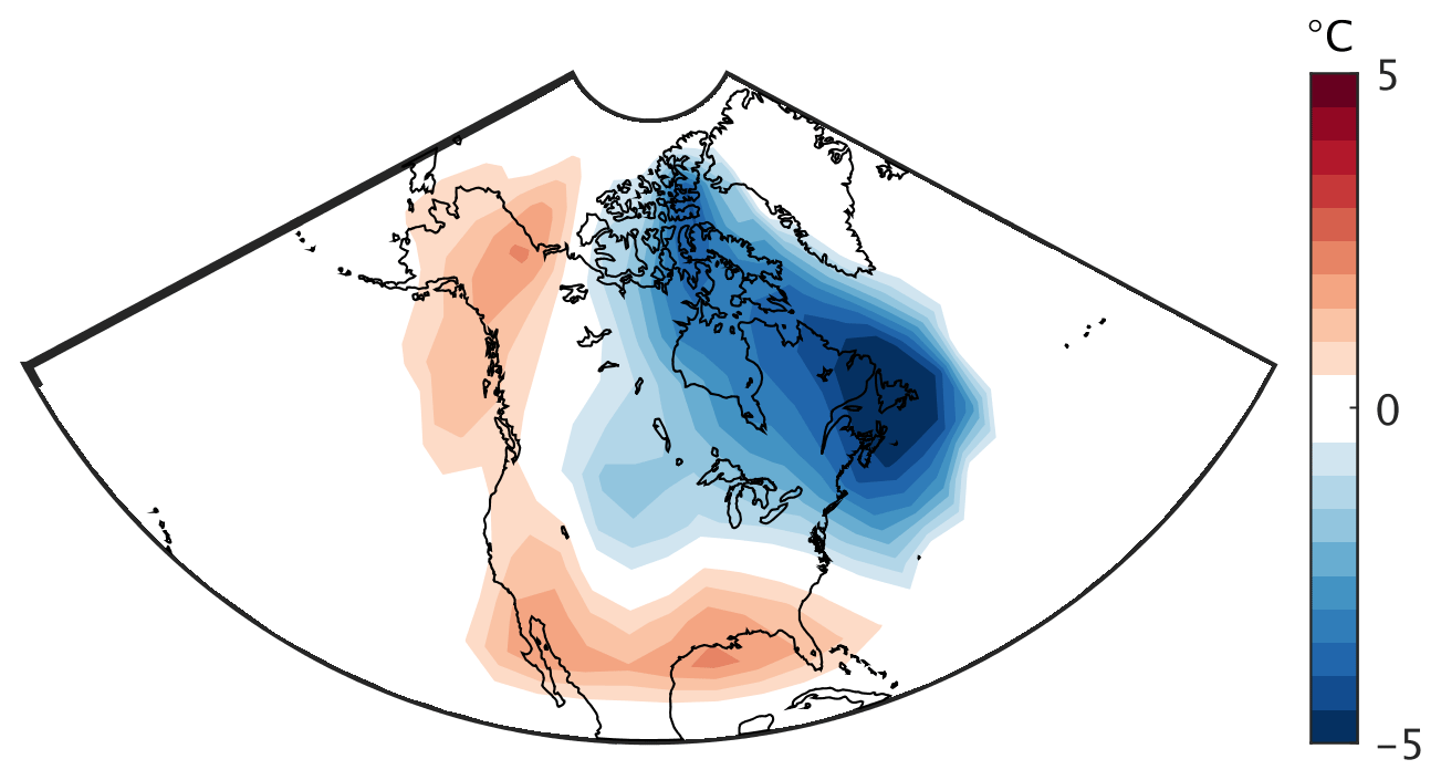
Figure B1 Temperature correction applied in SEMIX.

Furthermore, since the downwelling long-wave radiation at the surface, which also affects the surface energy balance, is closely related to near-surface air temperature, we also correct the downwelling long-wave radiation for the temperature bias using a simple quadratic relation derived from ERA5 reanalysis data (Fig.B2). Equation (B12) is then modified to

$$\begin{array}{}\text{(B14)}& \begin{array}{rl}{\mathrm{LW}}^{\downarrow }& ={\mathrm{LW}}^{\downarrow ,\mathrm{i}}+{{\displaystyle \frac{\partial {\mathrm{LW}}^{\downarrow }}{\partial z}}}^{\mathrm{i}}\left(z_{\mathrm{s}}-z_{\mathrm{s}}^{\mathrm{i}}\right)\\ & -(\mathrm{0.034}\cdot T_{\text{2m}}-\mathrm{5})\cdot T_{\text{2m,JJA}}^{{\text{bias}}^{\mathrm{i}}}.\end{array}\end{array}$$

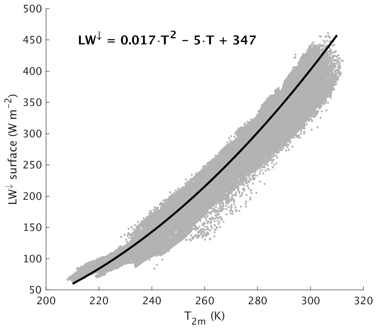
Figure B2 Scatterplot of downwelling long-wave radiation at the surface versus near-surface air temperature in the ERA5 reanalysis (Hersbach et al., 2020). The black line indicates the best quadratic fit to the data and the inset shows the corresponding quadratic equation, which is used for bias correction in the model.

Present-day annual precipitation simulated by CLIMBER-X over the region where ice sheets were growing during glacial inception is in reasonable agreement with observations (Fig.B3), and typical biases do not exceed 200 $\mathrm{kg}{\mathrm{m}}^{-\mathrm{2}}{\mathrm{yr}}^{-\mathrm{1}}$. At the same time, the effect of 1 °C summer temperature bias on annual snowmelt can be estimated using the classical positive degree day approach to be 200–500 $\mathrm{kg}{\mathrm{m}}^{-\mathrm{2}}{\mathrm{yr}}^{-\mathrm{1}}$. The low bound corresponds to a melt season duration of 2 months and parameter α = 3 $\mathrm{kg}{\mathrm{m}}^{-\mathrm{2}}\mathrm{°}{\mathrm{C}}^{-\mathrm{1}}{\mathrm{d}}^{-\mathrm{1}}$, while the upper bound corresponds to the melt season duration of 3 months and α = 5. Since simulated summer temperature biases are about 3–5 °C, temperature biases are much more important than precipitation biases. This is why we only correct the temperature and do not apply any corrections to precipitation.

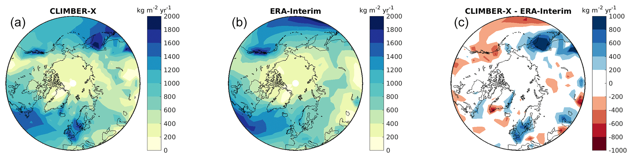
Figure B3 Simulated present-day annual precipitation in CLIMBER-X (a) compared to ERA-Interim reanalysis (Dee et al., 2011) (b). Panel (c) shows the precipitation bias in CLIMBER-X.

B3 Surface energy and mass balance of snow and ice

The surface energy balance in SEMIX is written as follows:

$$\begin{array}{}\text{(B15)}& {\mathrm{SW}}_{\mathrm{net}}+{\mathrm{LW}}^{\downarrow }-{\mathrm{LW}}^{\uparrow }-\mathrm{SH}-\mathrm{LE}-G=\mathrm{0},\end{array}$$

where SW_net is the net short-wave radiation absorbed at the surface, LW^↓ and LW^↑ are the downwelling and upwelling long-wave radiation at the surface, SH is the sensible heat flux, LE is the latent heat flux, and G the heat flux into the snow and ice. Equation (B15) is then solved for the skin temperature, T_skin, using the formulations for the energy fluxes described next.

The surface albedo values used to compute the net short-wave at the surface in Eq.B11 are defined as follows:

$$\begin{array}{}\text{(B16)}& {\displaystyle }{\mathit{\alpha }}_{\text{VIS,dir}}& {\displaystyle }=f_{\text{snow}}\cdot {\mathit{\alpha }}_{\text{VIS,dir}}^{\text{snow}}+(\mathrm{1}-f_{\text{snow}})\cdot {\mathit{\alpha }}^{\text{bg}},\text{(B17)}& {\displaystyle }{\mathit{\alpha }}_{\text{NIR,dir}}& {\displaystyle }=f_{\text{snow}}\cdot {\mathit{\alpha }}_{\text{NIR,dir}}^{\text{snow}}+(\mathrm{1}-f_{\text{snow}})\cdot {\mathit{\alpha }}^{\text{bg}},\text{(B18)}& {\displaystyle }{\mathit{\alpha }}_{\text{VIS,dif}}& {\displaystyle }=f_{\text{snow}}\cdot {\mathit{\alpha }}_{\text{VIS,dif}}^{\text{snow}}+(\mathrm{1}-f_{\text{snow}})\cdot {\mathit{\alpha }}^{\text{bg}},\text{(B19)}& {\displaystyle }{\mathit{\alpha }}_{\text{NIR,dif}}& {\displaystyle }=f_{\text{snow}}\cdot {\mathit{\alpha }}_{\text{NIR,dif}}^{\text{snow}}+(\mathrm{1}-f_{\text{snow}})\cdot {\mathit{\alpha }}^{\text{bg}},\end{array}$$

where the snow cover fraction f_snow is determined also considering the effect of topographic roughness following Niu and Yang (2007) and Roesch et al. (2001):

$$\begin{array}{}\text{(B20)}& f_{\text{snow}}=\tanh \left({\displaystyle \frac{h_{\text{snow}}}{\mathrm{10}\cdot z_{\mathrm{0}}}}\right){\displaystyle \frac{h_{\text{snow}}}{h_{\text{snow}}+\mathrm{2}\times {\mathrm{10}}^{-\mathrm{4}}\cdot {\mathit{\sigma }}_{\mathrm{z}}^{\mathrm{i}}}},\end{array}$$

where h_snow is snow thickness and z₀ is the surface roughness length. The snow albedo scheme is the same as used in the climate component of CLIMBER-X and includes a dependence on snow grain size and dust and soot concentration following Dang et al. (2015). The background albedo is a weighted average between a constant bare-soil albedo and variable ice albedo:

$$\begin{array}{}\text{(B21)}& {\mathit{\alpha }}_{\text{bg}}=f_{\text{ice}}\cdot {\mathit{\alpha }}^{\text{ice}}+(\mathrm{1}-f_{\text{ice}})\cdot {\mathit{\alpha }}^{\text{soil}}.\end{array}$$

The ice cover fraction is computed from ice sheet thickness, h_ice, and topographic roughness as:

$$\begin{array}{}\text{(B22)}& f_{\text{ice}}=\tanh \left({\displaystyle \frac{h_{\text{ice}}}{{\mathit{\sigma }}_{\mathrm{z}}^{\mathrm{i}}}}\right).\end{array}$$

For ice-free grid cells next to the ice sheet margin, where h_ice=0, an ice thickness is computed instead as an average over the 3 × 3 grid cells neighbourhood and will therefore by definition be >0. The ice albedo of newly formed ice is set to a constant value representative for firn, α^firn=0.7. As soon as ice starts to melt, the albedo gradually decreases towards a clean-ice albedo, assuming that the clean-ice albedo is reached when the firn layer is melted:

$$\begin{array}{}\text{(B23)}& {\displaystyle \frac{\mathrm{\Delta }{\mathit{\alpha }}^{\text{ice}}}{\mathrm{\Delta }t}}=-{\displaystyle \frac{{\mathit{\alpha }}^{\text{ice}}-{\mathit{\alpha }}_{\text{clean}}^{\text{ice}}}{h_{\text{firn}}{\mathit{\rho }}_{\text{firn}}/M_{\text{ice}}}},\end{array}$$

where M_ice is the rate of ice melt, h_firn is the constant thickness of the firn layer, and ρ_firn is the density of firn, which is also considered to be constant (Table B2). As the ice becomes snow free and therefore exposed to the deposition of dust and other wind-borne material that darken the ice, the albedo is assumed to decrease further towards a dirty-ice albedo, ${\mathit{\alpha }}_{\text{dirty}}^{\text{ice}}=\mathrm{0.4}$, with a timescale of 100 years. Whenever the annual surface mass balance is positive, indicating accumulation of snow and consequently formation of a firn layer, the ice albedo is reset to the albedo of firn (α^ice=α^firn). A few considerations are appropriate here on the representation of ice albedo in ice-free grid cells at the ice sheet margin. If the surface mass balance is positive in these points, the ice (or background) albedo is not very important because it implies that not all snow is melted during summer and therefore the background does not become exposed. On the other hand, if the surface mass balance is negative, the background albedo in the ice-free margin points should reflect the properties of the ice that could flow into these points from neighbouring grid cells through horizontal ice flow. In this case the ice albedo will determine how negative the mass balance is through its control on the absorbed radiation when all snow is melted. How negative the surface mass balance is will eventually determine whether the ice flowing into these grid cells will be melted completely or not and therefore plays a role in the velocity at which ice sheet cover can expand laterally. Based on these considerations the ice albedo in the grid cells at the ice sheet margin is computed as the average of the ice albedo of the neighbouring ice points.

Table B2 List of SEMIX model parameters.

The surface emitted long-wave radiation is given by the Stefan–Boltzmann law:

$$\begin{array}{}\text{(B24)}& {\mathrm{LW}}^{\uparrow }=\mathit{ϵ}\mathit{\sigma }{T}_{\text{skin}}^{\mathrm{4}},\end{array}$$

with ϵ the surface emissivity and σ the Stefan–Boltzmann constant.

The sensible heat flux is computed from the temperature gradient between the skin and near-surface air using the bulk aerodynamic formula:

$$\begin{array}{}\text{(B25)}& \mathrm{SH}={\displaystyle \frac{{\mathit{\rho }}_{\mathrm{a}}{c}_{\mathrm{p}}}{r_{\text{aer}}}}(T_{\text{skin}}-T_{\text{2m}}),\end{array}$$

where ρ_a is air density, c_p is the specific heat of air, and r_aer is the aerodynamic resistance. Similarly, the latent heat flux over sea ice is expressed in terms of the specific humidity gradient between the surface and near-surface air:

$$\begin{array}{}\text{(B26)}& \mathrm{LE}=L{\displaystyle \frac{{\mathit{\rho }}_{\mathrm{a}}}{r_{\text{aer}}}}\left(q_{\text{sat}}\right(T_{\text{skin}})-q_{\text{2m}}).\end{array}$$

L is the latent heat of sublimation and q_sat is the specific humidity at saturation. The aerodynamic resistance is computed from the wind speed, surface exchange coefficient, and bulk Richardson number following Willeit and Ganopolski (2016).

The conductive heat flux into the snow/ice (G) is computed as follows:

$$\begin{array}{}\text{(B27)}& G={\displaystyle \frac{\mathit{\lambda }}{\mathrm{\Delta }{z}_{\mathrm{1}}}}(T_{\text{skin}}-T_{\text{s,1}}),\end{array}$$

where λ is the heat conductivity of snow and ice and Δz₁ is the distance between the surface and the middle of the snow layer or uppermost ice layer with temperature T_s,1, depending whether a snow layer is present or not.

The prognostic terms in T_skin in the formulation of the surface energy fluxes are then linearized using Taylor series expansion assuming that the temperature at the new time step, $T_{\text{skin},n+\mathrm{1}}=T_{\text{skin},n}+\mathrm{\Delta }{T}_{\text{skin}}$ with ΔT_skin≪T_skin:

$$\begin{array}{}\text{(B28)}& {\displaystyle }{T}_{\text{skin},n+\mathrm{1}}^{\mathrm{4}}=T_{\text{skin},n}^{\mathrm{4}}+\mathrm{4}{T}_{\text{skin},n}^{\mathrm{3}}(T_{\text{skin},n+\mathrm{1}}-T_{\text{skin},n}),\text{(B29)}& {\displaystyle }\begin{array}{rl}{q}_{\text{sat}}\left(T_{\text{skin},n+\mathrm{1}}\right)& =q_{\text{sat}}\left(T_{\text{skin}}\right)+{\displaystyle \frac{\mathrm{d}{q}_{\text{sat}}}{\mathrm{d}{T}_{\text{skin}}}}{|}_{T_{\text{skin}}=T_{\text{skin},n}}\\ & \times (T_{\text{skin},n+\mathrm{1}}-T_{\text{skin},n}).\end{array}\end{array}$$

Equation (B15) can then be solved explicitly for the skin temperature at the new time step, $T_{\text{skin},n+\mathrm{1}}$. If the skin temperature is above freezing the surface energy fluxes are diagnosed first with the skin temperature greater then 0 °C and then with skin temperature set to 0 °C. The difference between the sum of the energy fluxes is then used to directly melt snow and/or ice, without the need for the snow or ice temperature to be at melting point.

The heat transfer in the snow–ice column is represented by a one-dimensional heat diffusion equation. A single snow layer is represented on top of five unevenly spaced vertical layers in the ice reaching a depth of 15 m. The heat flux G is applied as top boundary condition, while a no-flux condition is applied at the bottom of the ice column. If the temperature of the snow or ice layers is greater than 0 °C, the excess energy is used to melt snow or ice. Liquid water produced by snowmelt or added to the snow layer from rainfall can be refrozen in the snow layer or refreeze to form superimposed ice. The liquid water available for refreezing is

$$\begin{array}{}\text{(B30)}& F_{\text{avail}}=(M_{\text{snow}}+P_{\text{rain}})\mathrm{\Delta }t,\end{array}$$

where M_snow is snowmelt and Δt the time step in SEMIX (1 d). The maximum amount of water that is allowed to refreeze is taken to be a linear function of the thickness of the snow layer and accounts for the amount of water that has already been refrozen since the start of the melt season:

$$\begin{array}{}\text{(B31)}& F_{\text{max}}={\mathit{\varphi }}_{\text{snow}}{h}_{\text{snow}}{\mathit{\rho }}_{\text{snow}}-\sum F,\end{array}$$

where ϕ_snow is snow porosity, ρ_snow is snow density, and F is refreezing. The maximum amount of water available for refreezing then becomes

$$\begin{array}{}\text{(B32)}& F_{\text{avail}}^{\text{max}}=min(F_{\text{avail}},F_{\text{max}}).\end{array}$$

The amount of water that can potentially be refrozen depends on the “cold content” of the snow layer:

$$\begin{array}{}\text{(B33)}& F_{\text{pot}}={\displaystyle \frac{C_{\mathrm{i}}}{L_{\mathrm{f}}}}{h}_{\text{snow}}{\mathit{\rho }}_{\text{snow}}\cdot (T_{\mathrm{0}}-T_{\text{snow}}),\end{array}$$

with C_i the specific heat capacity of ice, L_f the latent heat of fusion, and T_snow the temperature of the snow layer. The actual refreezing rate is then simply the minimum between available and potential:

$$\begin{array}{}\text{(B34)}& F={\displaystyle \frac{min\left(F_{\text{avail}}^{\text{max}},F_{\text{pot}}\right)}{\mathrm{\Delta }t}}.\end{array}$$

A fraction f_rfz,snow is then assumed to refreeze within the snow layer, while the rest forms superimposed ice:

$$\begin{array}{}\text{(B35)}& f_{\text{rfz,snow}}=f_{\text{rfz,snow}}^{\text{max}}\cdot min\left(\mathrm{1},{\displaystyle \frac{h_{\text{snow}}}{h_{\text{snow}}^{\text{crit}}}}\right),\end{array}$$

where $f_{\text{rfz,snow}}^{\text{max}}$ and $h_{\text{snow}}^{\text{crit}}$ are model parameters (Table B2).

Finally, the surface mass balance and runoff are diagnosed as follows:

$$\begin{array}{}\text{(B36)}& {\displaystyle }& {\displaystyle }\mathrm{SMB}=P_{\text{snow}}-E-M_{\text{snow}}-M_{\text{ice}}+F\text{(B37)}& {\displaystyle }& {\displaystyle }R=M_{\text{snow}}+M_{\text{ice}}+P_{\text{rain}}-F.\end{array}$$

These are then integrated over the whole year and passed to the ice sheet model. The surface ice temperature, which is needed by the ice sheet model as top boundary condition in the temperature equation, is computed as the annual average temperature of the deepest ice layer (∼ 10 m).

Appendix C: IMO ice shelf basal melt model

In CLIMBER-X we have implemented the simple and general ice shelf basal melt parameterizations of Beckmann and Goosse (2003) and Pollard and Deconto (2012), both of which rely on the difference between the ambient water temperature derived from ocean or lake model and the freezing point temperature at the ice shelf base.

The basal mass balance in the linear model of Beckmann and Goosse (2003) is

$$\begin{array}{}\text{(C1)}& \mathrm{BMB}=k_{\mathrm{1}}{\displaystyle \frac{{\mathit{\rho }}_{\mathrm{w}}{C}_{\mathrm{w}}}{{\mathit{\rho }}_{\mathrm{i}}{L}_{\mathrm{f}}}}(T_{\mathrm{w}}-T_{\mathrm{f}}),\end{array}$$

where k₁ is a model parameter (Table C1), ρ_w is a typical seawater density, C_w is the specific heat capacity of water, ρ_i is the density of ice, and L_f is the latent heat of fusion of ice. T_w is either the seawater temperature from the ocean model for marine-terminating margins or the lake water temperature for lake-terminating margins, horizontally extrapolated to the ice sheet model grid and vertically interpolated to the depth of the ice shelf base. T_f is the freezing point temperature at the base of the ice shelf (Beckmann and Goosse, 2003):

$$\begin{array}{}\text{(C2)}& T_{\mathrm{f}}=\mathrm{0.0939}-\mathrm{0.057}\cdot S_{\mathrm{w}}-\mathrm{7.64}\times {\mathrm{10}}^{-\mathrm{4}}\cdot z_{\mathrm{b}},\end{array}$$

where S_w is the water salinity, derived similarly to T_w, assuming that the salinity of lakes is zero, and z_b is the depth of the ice shelf base below sea level.

The basal mass balance in the model of Pollard and Deconto (2012) is similar but relies on a quadratic dependence on the temperature gradient:

$$\begin{array}{}\text{(C3)}& \mathrm{BMB}=k_{\mathrm{2}}{\displaystyle \frac{{\mathit{\rho }}_{\mathrm{w}}{C}_{\mathrm{w}}}{{\mathit{\rho }}_{\mathrm{i}}{L}_{\mathrm{f}}}}\left|T_{\mathrm{w}}-T_{\mathrm{f}}\right|\cdot (T_{\mathrm{w}}-T_{\mathrm{f}}),\end{array}$$

where k₂ is a model parameter; all other terms in this equation have already been defined above.

Similarly to Quiquet et al. (2021), in order to avoid unrealistic ice shelf expansion over the deep ocean, we apply an additional scaling of basal melt with the depth of the bedrock elevation:

$$\begin{array}{}\text{(C4)}& f_{\mathrm{BMB}}=\mathrm{1}+{\displaystyle \frac{max\left(\mathrm{0},z_{\text{bed}}-z_{\text{bed}}^{\text{ref}}\right)}{z_{\text{bed}}^{\text{ref}}}},\end{array}$$

with $z_{\text{bed}}^{\text{ref}}$ being a model parameter (Table C1).

IMO is called every month to resolve the seasonal cycle in ocean and lake temperature, but the coupling with the ice sheet model is done yearly.

Beckmann and Goosse (2003)Pollard and Deconto (2012)

Table C1 List of IMO model parameters.

Appendix D: VILMA solid Earth model

The solid Earth model VILMA solves the field equations of a viscoelastic incompressible and self-gravitating continuum in the spherical domain for the mantle and lithosphere of the Earth. The fluid core and loading processes at the surface are considered boundary conditions at the respective boundaries. Lateral changes in viscosity are considered and are following the formulation as an initial value problem discussed in Martinec (2000): the field equations are solved in the spherical harmonic domain but integrated over time with an explicit time differencing scheme. In view of solving the momentum equation in the spectral solution, the code is rather efficient and in view of the time-differencing scheme the coupling with the Earth system model is straightforward (Konrad et al., 2015). The loading is considered as a pressure field boundary condition applied at the surface, where mass conservation is considered solving the sea level equation (Farrell and Clark, 1976) at each time step. The time step interval is constrained by the minimum ratio of viscosity versus shear modulus (the Maxwell time). It is usually about 20 years for a standard Earth structure but has to be reduced to about 1 year for a 3D structure containing structural features like low viscous regions in tectonically active regions. For the 3D viscosity field in this study we chose the 3D model v₁.0_s16 from Bagge et al. (2021) (Fig. D1) as it shows the smallest misfit with observational data in independent GIA models. In the present work we set a minimum viscosity of 10^19.5, which allows a time step of 10 years to be used. Due to the fact that the time step is rather small, an iteration at each time step as discussed in Kendall et al. (2005) can be neglected.

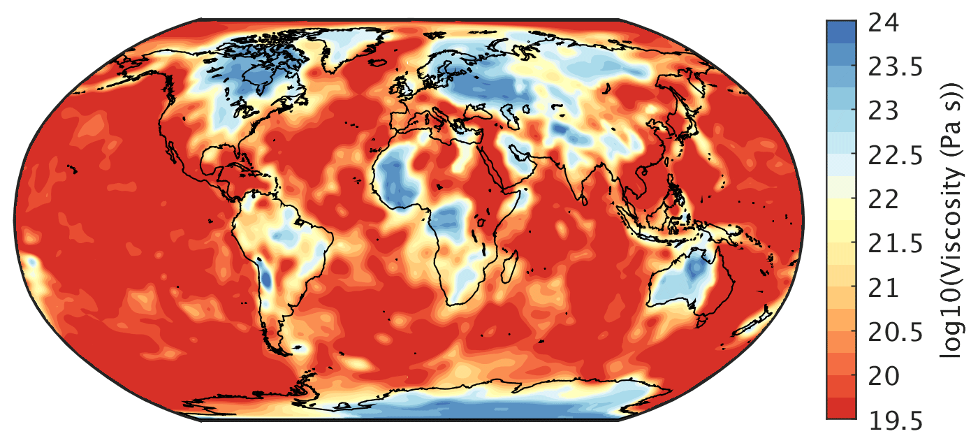
Figure D1 Viscosity at 200 km depth from Bagge et al. (2021) as used in the model simulations.

The relative sea level determined by VILMA is used as the spatially variable correction of the considered reference topography, h_topo(t₀). In this way, changes in the topography are considered with respect to the changing geoid defined here as the mean sea level at the respective time step:

$$\begin{array}{}\text{(D1)}& h_{\text{topo}}\left(t\right)=h_{\text{topo}}\left(t_{\mathrm{0}}\right)-h_{\text{rsl}}(t-t_{\mathrm{0}}),h_{\text{rsl}}\left(t_{\mathrm{0}}\right)=\mathrm{0}.\end{array}$$

This view is consistent with the natural definition of topography in the understanding of Carl Friedrich Gauss. It also means that all changes in elevation are expressed as measured relative to the mean sea level at that time.

Changes in topography due to variations in sea level are considered furthermore by updating the land–sea mask at each time step. This holds also for the conditions of floating versus grounded ice. In view of completing formulations (e.g. Kendall et al., 2005; Spada and Melini, 2019), the effect of rotational deformations was implemented recently in VILMA following the formulation of Martinec and Hagedoorn (2014). Rotational deformations have to be considered, especially when discussing the effect of GIA on geodetic observables like GNSS, EOP, and gravity or when discussing future sea level changes (e.g. Palmer et al., 2020).