Bayesian multi-proxy reconstruction of early Eocene latitudinal temperature gradients

Accurately reconstructing large-scale palaeoclimatic patterns from sparse local records is critical for understanding the evolution of Earth's climate. Particular challenges arise from the patchiness, uneven spatial distribution, and disparate nature of palaeoclimatic proxy records. Geochemical data typically provide temperature estimates via transfer functions derived from experiments. Similarly, transfer functions based on the climatic requirements of modern taxa exist for some fossil groups, such as pollen assemblages. In contrast, most ecological and lithological data (e.g. coral reefs and evaporites) only convey information on broad climatic requirements. Historically, most large-scale proxy-based reconstructions have used either geochemical or ecological data, but few studies have combined multiple proxy types into a single quantitative reconstruction. Large spatial gaps in existing proxy records have often been bridged by simple averaging, without taking into account the spatial distribution of samples, leading to biased temperature reconstructions. Here, we present a Bayesian hierarchical model to integrate ecological data with established geochemical proxies into a unified quantitative framework, bridging gaps in the latitudinal coverage of proxy data. We apply this approach to the early Eocene climatic optimum (EECO), the interval with the warmest sustained temperatures of the Cenozoic. Assuming the conservation of thermal tolerances of modern coral reefs and mangrove taxa, we establish broad sea surface temperature ranges for EECO coral reef and mangrove sites. We integrate these temperature estimates with the EECO geochemical shallow marine proxy record to model the latitudinal sea surface temperature gradient and global average temperatures of the EECO. Our results confirm the presence of a flattened latitudinal temperature gradient and unusually high polar temperatures during the EECO, which is supported by high-latitude ecological data. We show that integrating multiple types of proxy data, and adequate prior information, has the potential to enhance quantitative palaeoclimatic reconstructions, improving temperature estimates from datasets with limited spatial sampling.

1 Introduction

Understanding the long-term evolution of Earth's climate system and contextualising contemporary global warming relies on accurate reconstructions of past climates (Royer et al., 2004; Burke et al., 2018; Tierney et al., 2020). Recent advances in the synthesis of palaeoclimatic data (e.g. Veizer and Prokoph, 2015; Hollis et al., 2019; Song et al., 2019; Grossman and Joachimski, 2022; Judd et al., 2022) are offering unprecedented insights into the complex and dynamic nature of the Earth's climate system, yet a fundamental challenge remains: the proxy record of past climates is spatially incomplete and afflicted by imperfect preservation and uneven sampling (Judd et al., 2020; Jones and Eichenseer, 2022; Judd et al., 2022).

Acknowledging the assumptions and limitations inherent in geochemical temperature proxies, such as experimentally derived calibrations, influences from seasonality, dissolution effects, and differential preservation (e.g. Tierney et al., 2017), can enable robust estimates of palaeotemperature at local scales. However, recent work has demonstrated that spatial biases in the geochemical proxy record can lead to spurious estimates of regional (e.g. latitudinal temperature gradients) and global temperatures (Judd et al., 2020; Jones and Eichenseer, 2022). Principally, this can be driven by two factors: (1) missing data for some regions (e.g. no high-latitude data); or (2) overrepresentation of other regions (e.g. a high proportion of samples from tropical areas). The latter can be addressed through the downsampling of data or restricting analyses to specific regions (e.g. Song et al., 2019). However, in order to robustly infer regional or global-scale patterns from an incomplete record, spatial gaps must ultimately be bridged. One common approach, which requires no additional computation, is the spatial visualisation of proxy-derived temperatures against latitude, showing broad latitudinal temperature trends (e.g. Hollis et al., 2019; Vickers et al., 2021). Interpolation is also sometimes used to bridge spatial gaps in palaeoclimatic data (e.g. Taylor et al., 2004), taking advantage of the autoregressive nature of climatic data: much of the information on the climate of any given location is contained in the climate data of nearby locations (Reynolds and Smith, 1994). Adding to this, some proxy-based reconstructions use statistical modelling to infer palaeoclimatic patterns. For example, polynomial regression (Bijl et al., 2009) and cosine functions (Inglis et al., 2020) have been used to reconstruct latitudinal temperature gradients, and 2D reconstructions of surface temperatures have been created with Gaussian process regression (Inglis et al., 2020). These approaches work well for interpolating relatively densely sampled data, but the absence of constraints on the modelled parameters means that such models can produce unrealistic temperature estimates when extrapolating from sparse data. Statistical modelling in a Bayesian framework can help overcome this problem by requiring the explicit specification of priors for the model parameters, which can be used to express physical constraints (Chandra et al., 2021).

Spatial gaps in the palaeoclimatic record can also be addressed through the integration of additional data. For example, lithological and fossil data can be used to infer past climatic conditions based on analogous modern sediments (Chandra et al., 2021), or based on the premise that the climatic requirements of ancient taxa, biological traits, or ecological communities were similar to those of their nearest modern relatives (Peppe et al., 2011; Royer, 2012; Salonen et al., 2019). Despite this potential, the integration of geochemical proxy data with other sources of information (e.g. ecological data) has rarely been realised in a rigorous, quantitative framework (Burgener et al., 2023).

Here, we present a novel Bayesian hierarchical model (e.g. Gelman et al., 2013; McElreath, 2018) that combines quantitative proxies and ecological constraints into a fully quantitative model of the latitudinal gradient of sea surface temperatures, bridging spatial gaps in sparsely sampled palaeoclimatic data. The Bayesian approach offers a powerful framework for integrating various sources of uncertainty and modelling complex hierarchical relationships and is increasingly used in palaeoclimatic reconstructions (e.g. Weitzel et al., 2019; Yang and Bowen, 2022; Burgener et al., 2023). This model expands upon existing, spatially explicit palaeoclimatic reconstructions by allowing for the integration of (1) prior information based on physical principles and the observed modern sea surface temperature distribution and of (2) geochemical and ecological palaeoclimatic proxies in a common quantitative framework. We chose a generalised logistic function to accurately infer the shape of the temperature gradient despite a patchy latitudinal coverage. This choice is motivated by the flexibility and ability of this function to approximate a variety of nonlinear patterns in the underlying temperature gradients that other parametric approaches, such as lower-order polynomials (e.g. Bijl et al., 2009; Keating-Bitonti et al., 2011), lack. We test the robustness of this method using downsampled, simulated latitudinal temperature gradients.

Table 1 Inferred latitudinal sea surface temperature (SST) gradients for the early Eocene (EE) or the EECO, as shown in earlier proxy-based studies. The gradient values denote the SST difference between the Equator and the polar circle or other types of gradients. For comparison, a gradient derived from an atmosphere–ocean general circulation model (GCM) ensemble and a range of gradients from a model intercomparison project are also shown.

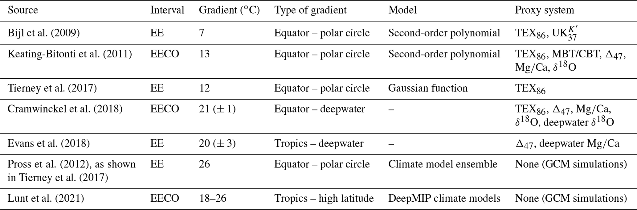
We apply this model to the record of the early Eocene climatic optimum (EECO), combining a compilation of geochemical proxies (Hollis et al., 2019), mangrove communities (Popescu et al., 2021), and coral reefs (Zamagni et al., 2012). We use a nearest-living-relative approach (e.g. Greenwood et al., 2017) to establish broad temperature ranges for the ecological data. We choose the EECO to demonstrate the application of the model due to its significance as the interval with the warmest sustained temperatures of the Cenozoic (Pross et al., 2012), rendering it a potential analogue for extreme climate warming scenarios (Burke et al., 2018). Our integrative approach allows us to shed new light on the long-standing dispute on the steepness of the early Eocene temperature gradient (Table 1; Sloan and Barron, 1990; Markwick, 1994; Huber and Caballero, 2011; Tierney et al., 2017; Inglis et al., 2020).

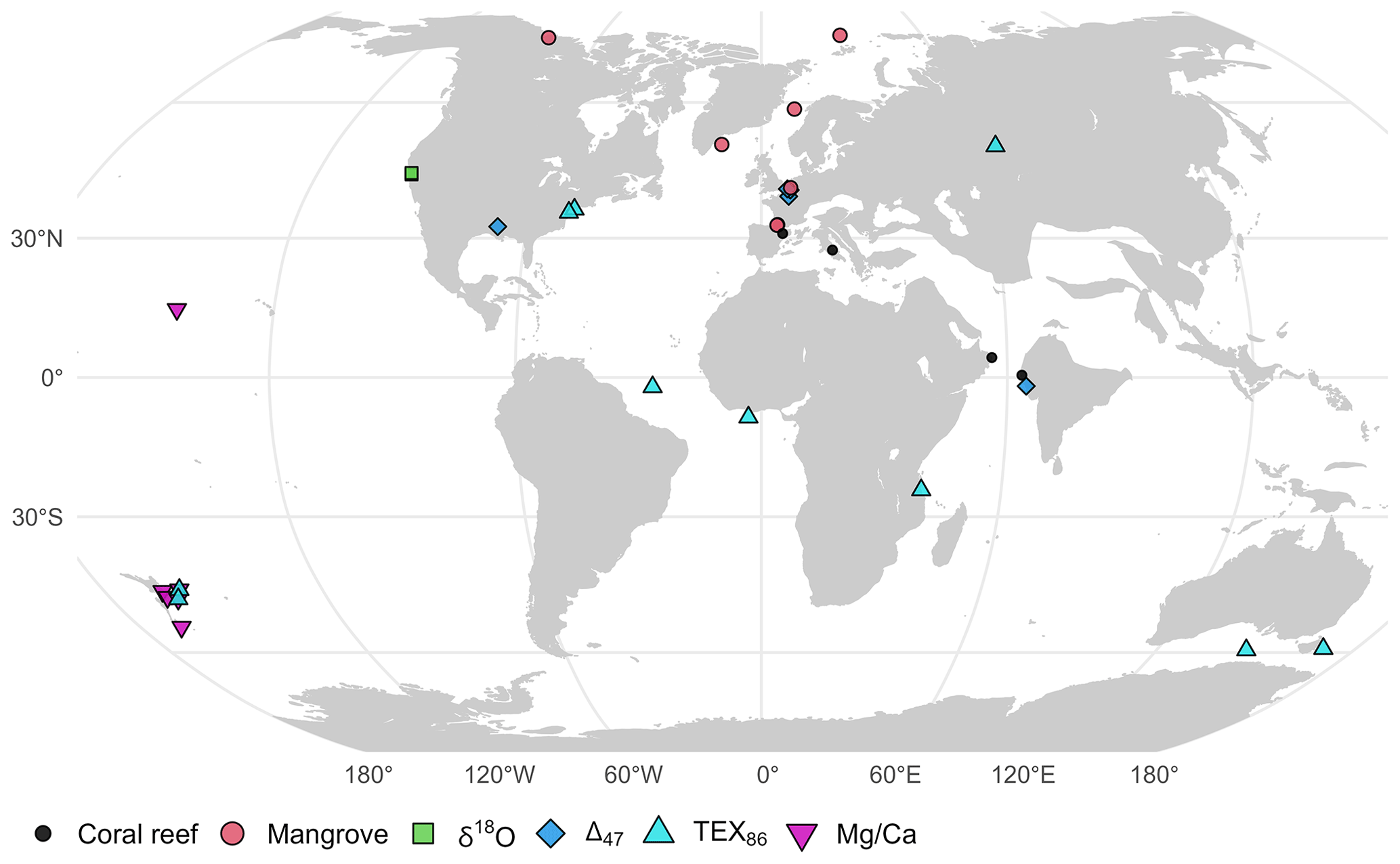
Figure 1 Palaeogeographic distribution of the geochemical and ecological data compilation used in this study. Map is presented in the Robinson projection (ESRI:54030). Palaeogeographic reconstructions were computed using the Merdith et al. (2021) Global Plate Model via the palaeoverse R package (Jones et al., 2023) and GPlates Web Service (https://gwsdoc.gplates.org, last access: 14 September 2023).

2 Materials and methods

2.1 Geochemical data

Geochemical climatic proxy data were extracted from a latest Paleocene and early Eocene compilation (Hollis et al., 2019). This compilation provides sea surface temperature data on four different geochemical proxies for reconstructing seawater temperature: δ¹⁸O, Δ₄₇, $\mathrm{Mg}/\mathrm{Ca}$, and TEX₈₆. For our analyses, this dataset was restricted to the EECO (defined as 53.8–49.1 Ma) and samples originating from near the ocean surface or mixed layer. Consequently, samples labelled “thermocline” or “sub-thermocline” were excluded. Recrystallised δ¹⁸O samples were also excluded, as secondary diagenetic calcite precipitated after deposition can bias isotope measurements and offset temperature values (Schrag, 1999). This filtering resulted in most δ¹⁸O samples being excluded from the dataset (retaining 8 out of 152). After data filtering, 308 geochemical proxy samples from 23 locations remained (Fig. 1). For a detailed description of each proxy, see Hollis et al. (2019).

2.2 Ecological data

2.2.1 Coral reefs

Today, shallow warm-water coral reefs are limited to tropical and subtropical latitudes (∼ 34^∘ N–32^∘ S), with minimum sea surface temperature tolerances (∼ 18 ^∘C) being the primary constraint on this distribution (Johannes et al., 1983; Kleypas et al., 1999; Yamano et al., 2001). As coral reefs reside at the upper thermal limit of the oceans today, their maximum sea surface temperature tolerance is less well-constrained, with some studies suggesting up to 35.6 ^∘C in the geological past (Jones et al., 2022). Nevertheless, coral reefs have frequently been recognised as tracers of past (sub-)tropical conditions (Ziegler et al., 1984; Kiessling, 2001). During the Eocene, coral communities and reefs expanded across tropical and temperate latitudes, with communities found up to palaeolatitudes of 43^∘ N (Zamagni et al., 2012). Using a compilation of Paleocene–early Eocene coral reefs and community localities (Zamagni et al., 2012), we generated quantitative sea surface temperature estimates for the EECO. To do so, we extracted localities from the compilation that are inferred to be Ilerdian (early Eocene) coral reefs and that could be confidently assigned to the EECO. We excluded coral knobs and coral-bearing mounds, which might have broader climatic limits than warm-water coral reef ecosystems. This filtering resulted in four unique coral reef localities remaining for the EECO, all of which conform to the modern latitudinal range of coral reefs (< 34^∘ N). Subsequently, we used statistically derived temperature limits (minimum = 21 ^∘C; average = 27.6 ^∘C; maximum = 29.5 ^∘C) from the published literature (Kleypas et al., 1999) to define a normal probability distribution of potential temperature values for coral reef localities. This normal probability distribution was defined with a mean of 27.6 ^∘C and a standard deviation of 2.125 ^∘C, which places the minimum (21 ^∘C) at the lower end of the 95 % highest density interval of that distribution. As the distribution of modern corals is skewed towards warmer temperatures, this approach results in 16.5 % of the probability being placed on temperatures > 29.5 ^∘C, allowing for the possibility that Eocene coral reefs were adapted to warmer conditions than present-day coral reefs.

2.2.2 Mangroves

Mangroves are distributed throughout the tropics and subtropics today. While factors besides sea surface temperatures (SSTs) influence the distribution of mangroves, empirical lower temperature limits have been established for the genera Avicennia (15.6 ^∘C) and Rhizophora (20.7 ^∘C) (Quisthoudt et al., 2012). Both Avicennia and members of the Rhizophoraceae family were widespread and co-occurred across tropical and temperate latitudes in the early Eocene. Only Avicennia, however, occurred at polar latitudes (Suan et al., 2017; Popescu et al., 2021). Assuming that Eocene members of these mangrove taxa conform to similar climatic requirements to those of their modern relatives, the presence and absence of Avicennia and Rhizophoraceae pollen can be used as a palaeotemperature indicator. For this analysis, published mangrove occurrence data were taken from Popescu et al. (2021) and converted to quantitative temperature estimates. From these data, we identify two types of pollen assemblages which we ascribe different temperature distributions.

• Avicennia-only assemblages (n=2). The absence of Rhizophoraceae is indicative of temperatures between 15.6 ^∘C (lower temperature limit of Avicennia) and 20.7 ^∘C (lower temperature limit of Rhizophora). However, a value of 22.5 ^∘C is assumed as the upper temperature limit here, as Rhizophora is rare below this temperature. We define the Avicennia-only temperature distribution as being a normal distribution with a mean of 19.05 ^∘C and a standard deviation of 1.725 ^∘C, resulting in 95 % of the probability density being placed within the temperature limits.

• Avicennia and Rhizophoraceae assemblages (n=5). The presence of both groups suggests that the locality should have a minimum temperature of 20.7 ^∘C (lower temperature limit of Rhizophora). As the upper thermal limits of Avicennia and Rhizophora are not well established in Quisthoudt et al. (2012), we assign the same maximum temperature limits (29.5 ^∘C) as the coral reef localities because mangroves are also widely distributed throughout tropical regions. Consequently, we define the temperature distribution for this locality as a normal distribution, with a mean of 25.1 ^∘C, and a standard deviation of 2.2 ^∘C, with 95 % probability density within the temperature limits.

2.3 Palaeogeographic reconstruction

The palaeogeographic distribution of geochemical and ecological data was reconstructed using the Merdith et al. (2021) Global Plate Model via the palaeoverse R package (version 1.2.0, Jones et al., 2023). The midpoint age of the EECO (51.2 Ma), along with the present-day coordinates of geochemical and ecological data, were used for palaeogeographic reconstruction.

2.4 Bayesian framework

2.4.1 Model structure

We model the mean temperature (μ) at location j as a function of absolute latitude (abs(l)) with a logistic regression (also known as growth curve or Richard's curve) of the following form:

$$\begin{array}{}\text{(1)}& {\displaystyle }{\mathit{\mu }}_j\sim N({\mathit{\nu }}_j,\mathit{\sigma }),\text{(2)}& {\displaystyle }{\mathit{\nu }}_j=A+{\displaystyle \frac{K-A}{\mathrm{1}+e^{B\left(\text{abs}\right(l_j)-M)}}}j=\mathrm{1},\mathrm{\dots },n,\end{array}$$

where A and K denote the lower and upper asymptote, respectively; M specifies the latitude of maximal growth (i.e. the latitude around which temperature falls most steeply with latitude); B denotes the growth rate; σ denotes the residual standard deviation; and n denotes the number of locations.

We use this generalised logistic function because it can follow the equatorial and polar asymptotes observed in the modern latitudinal SST gradient, but can also accommodate a variety of other shapes, while consisting of only four shape parameters. This flexibility is primarily achieved by shifting the location of the curve along the latitudinal axis by varying M and by altering the steepness of the curve by varying B. For example, one limb of a second-order polynomial, as in Bijl et al. (2009), can be approximated by increasing M towards high latitudes and decreasing B to reduce the steepness of the curve. The model is designed for modelling the average gradient across both hemispheres but can also be applied to individual hemispheres to assess hemispherical differences (see Fig. S4).

We infer μ_j from m individual temperature observations $t_{i=\mathrm{1},\mathrm{\dots },m}$, derived from geochemical data, at location j as

$$\begin{array}{}\text{(3)}& t_{i,j}\sim N({\mathit{\mu }}_j,{\mathit{\sigma }}_j)i=\mathrm{1},\mathrm{\dots },m,\end{array}$$

where m is the number of observations at each location, and σ_j is the estimated standard deviation of the temperatures at location j.

Similarly, μ_j is inferred for locations with ecological proxies from the associated normal temperature distributions with a given mean and standard deviation, t_μ,j and t_σ,j, as

$$\begin{array}{}\text{(4)}& t_{\mathit{\mu },j}\sim N({\mathit{\mu }}_j,t_{\mathit{\sigma },j}).\end{array}$$

This structure implies that μ_j is not fixed at the mean proxy temperature at location j but is drawn towards the overall logistic regression curve, i.e. towards ν_j. The pull towards ν_j tends to be strong when m is low, when the observations $t_{i=\mathrm{1},\mathrm{\dots },m,j}$ are scattered, i.e. σ_j is high, and/or when the overall standard deviation σ is low. In practice, this has the desirable consequence that locations with few observations and large temperature differences between observations have less influence on the overall regression than well-sampled locations with consistent reconstructed temperatures.

We show an expanded model that includes uncertainties about individual temperature observations in the Supplement (Fig. S5).

2.4.2 Priors

In a Bayesian framework, priors need to be placed on the unknown parameters of a model. We placed weakly informative, conjugate inverse-gamma priors on σ and ${\mathit{\sigma }}_{j=\mathrm{1},\mathrm{\dots },n}$:

$$\begin{array}{}\text{(5)}& {\displaystyle }\begin{array}{rl}\mathit{\sigma }\sim & \sqrt{\text{inv-gamma}\left(\mathit{\alpha }+{\displaystyle \frac{n}{\mathrm{2}}},\mathit{\beta }+\mathrm{0.5}\times ({\mathit{\mu }}_j-{\mathit{\nu }}_j)\right)}\\ & j=\mathrm{1},\mathrm{\dots },n,\end{array}\text{(6)}& {\displaystyle }\begin{array}{rl}{\mathit{\sigma }}_j\sim & \sqrt{\text{inv-gamma}\left(\mathit{\alpha }+{\displaystyle \frac{m}{\mathrm{2}}},\mathit{\beta }+\mathrm{0.5}\times (t_{i,j}-{\mathit{\mu }}_j)\right)}\\ & i=\mathrm{1},\mathrm{\dots },m,j=\mathrm{1},\mathrm{\dots },n.\end{array}\end{array}$$

We set $\mathit{\alpha }=\mathit{\beta }=\mathrm{1}$, allowing these priors to be quickly overwhelmed by the data as n and m increase, as we have little a priori knowledge of these parameters.

In contrast, we put informative priors on the regression coefficients A, K, M, and B, based on physical principles and loosely based on the modern climate system.

• A. Predicted seawater surface temperatures are not allowed to be ≪ −2 ^∘C, which is the freezing point of seawater. The highest prior density of A is placed around 0 ^∘C, and it slowly tapers off towards higher temperatures. This shape is achieved by placing a skew-normal (SN) prior on the lower asymptote, specified as

  $$\begin{array}{}\text{(7)}& A\sim \text{SN}(\mathit{\xi }=-\mathrm{3.0},\mathit{\omega }=\mathrm{12},{\mathit{\alpha }}_{\text{SN}}=\mathrm{30}),\end{array}$$

  where ξ, ω, and α_SN are the location, scale, and shape parameters.

• K. Input of solar energy decreases from the tropics to the poles. Hence, the latitudinal temperature gradient is broadly negative, i.e. temperature decreases with absolute latitude. This is achieved by setting K≥A. The prior on the upper asymptote K is a truncated normal distribution, with the mean set to K of the modern SST gradient, with a broad standard deviation:

  $$\begin{array}{}\text{(8)}& K\sim \text{TN}({\mathit{\mu }}_{\text{TN}}=\mathrm{28},{\mathit{\sigma }}_{\text{TN}}=\mathrm{15},{\mathit{\alpha }}_{\text{TN}}=A,{\mathit{\beta }}_{\text{TN}}=\mathrm{\infty }).\end{array}$$

  The distribution is truncated to the left at α_TN=A but not truncated to the right (β_TN).

• M. A uniform prior is placed on the latitude of greatest steepness of the gradient, allowing it to be steepest anywhere between latitudes 0 and 90^∘ absolute latitude, as this parameter may vary greatly, depending on the climate state:

  $$\begin{array}{}\text{(9)}& M\sim \text{uniform}(\mathrm{0},\mathrm{90}).\end{array}$$

• B. The steepness or growth rate B of the gradient is constrained to be ≥0 and to not be exceedingly high, as oceanic and atmospheric heat transfer is bound to limit very abrupt SST changes across latitudes on a global scale. A gamma-distributed prior of the form

  $$\begin{array}{}\text{(10)}& B\sim \text{Gamma}({\mathit{\alpha }}_{\mathrm{G}}=\mathrm{4.3},{\mathit{\beta }}_{\mathrm{G}}=\mathrm{30})\end{array}$$

  was placed on B. The shape and rate parameters α_G and β_G were chosen such that the highest prior density is at B of the modern SST gradient, 0.11. We informed the prior distribution on B based on a provisional model run with the modern SST data.

2.5 Model validation

To test whether our logistic regression model can adequately describe different latitudinal temperature gradients at various sample sizes, we used the empirical modern gradient, representative of an icehouse climate, and generated three idealised gradients that emulate potential climatic states throughout Earth's geological history: extreme icehouse, icehouse (modern), greenhouse, and extreme greenhouse (Frakes et al., 1992). The idealised gradients serve to test whether our model set-up is able to infer gradients that are strongly different from the modern from a varying number of samples.

We created test data from these gradients as follows. We randomly sampled (1000 iterations) latitudes at sample sizes of 5, 10, and 20, with the probability of a latitude being sampled scaling with the decreasing surface area towards higher latitudes; i.e. lower latitudes are sampled more frequently. For the largest sample size (n = 34), we used the latitudes of the EECO dataset of this study in all iterations. For each latitude, we took the location mean temperature from the gradients, adding random noise from a normal distribution with a standard deviation of 3.8, which corresponds to the average uncertainty associated with the EECO geochemical proxy data (Hollis et al., 2019). With that, we aim to simulate randomly distributed errors in the proxy data, which could arise from miscalibration, measurement errors, seasonal effects, etc. We acknowledge that this approach cannot quantify the potential impact of systematic offsets that may bias all proxy data in the same direction, nor do we know whether a standard deviation of 3.8 is the actual average magnitude of uncertainty that the proxy compilation is afflicted with.

To evaluate how well the model performed in reconstructing the idealised gradients from limited sampling, we calculated the coefficient of determination (R²) for Bayesian regression models (Gelman et al., 2019). For every iteration from the posterior, we intercepted the modelled and the idealised gradient in intervals of 1^∘ latitude and calculated the R² based on these values. We report the median and 95 % credible intervals (CIs) of the resulting R² values. Here and in all other instances, the 95 % CIs refer to the interval between the 2.5 % point and the 97.5 % point of the samples or sampled posterior distribution.

To test whether our model can accurately depict the shape of the modern sea surface temperature gradient, and to facilitate comparison with the Eocene gradient, we applied our model to mean annual sea surface temperatures from Bio-ORACLE (Assis et al., 2018), aggregated to a spatial grid resolution of 1^∘ × 1^∘ (n = 46 131). The R² for the modern gradient was calculated as above (Gelman et al., 2019), comparing the modelled gradient and the empirical temperature averages in 1^∘ latitude bins. Only the medians are reported for the modern gradient, as the 95 % credible intervals are extremely narrow, due to the high precision of the posterior estimates.

To reconstruct the idealised gradients and the modern gradient, we used a simplified, non-hierarchical version of our model, as every location is associated with only one temperature value, making the hierarchical structure superfluous. To achieve this, we substituted temperature (t_j) for μ_j in Eqs. (1) and (5).

2.6 Parameter estimation

We estimated the posterior distributions of the model parameters using a Markov chain Monte Carlo (MCMC) algorithm, written in R (R Core Team, 2023). Specifically, we sampled the unknown parameters A, K, M, and B with Metropolis–Hastings and used Gibbs sampling to estimate all other unknown parameters (see Gilks et al., 1995; Gelman et al., 2013). Posterior inference on the modern gradient is based on four chains with 60 000 iterations each, 10 000 of which were discarded as burn-in. Every 10th iteration was retained, resulting in a total of 20 000 iterations with low autocorrelation. The resampled simulated gradients and the resampled modern gradient were modelled in one chain, with 10 000 iterations for each of the 1000 random samples. In each run, 5000 iterations each were discarded as burn-in, and every 25th iteration was kept, resulting in a total of 200 000 iterations across all 1000 model runs. For the Eocene model, we ran four chains with 600 000 iterations each, discarding 100 000 as burn-in and keeping every 100th iteration, as the hierarchical model structure results in higher autocorrelation of the chains. The Eocene posterior inference is thus based on a total of 20 000 iterations with low autocorrelation (effective multivariate sample size for A, K, M, and B is > 18 000). Trace plots of the MCMC chains indicate convergence and good mixing of the chains (Fig. S1 in the Supplement).

2.7 Processing of model results

Modelled sea surface temperature estimates were generated with Eq. (2), calculating the sea surface temperatures at any latitude with the parameter estimates of each iteration from the posterior samples. The median and 95 % CI of temperatures were then taken from all temperature estimates obtained at the latitudes of interest.

The latitudinal gradient was calculated as the difference between the modelled temperature at the Equator (0^∘ latitude) and at the poles (90^∘ absolute latitude). To facilitate comparison with earlier estimates, we also calculated the gradient with the temperature at the polar circle (66.6^∘ absolute latitude) being used instead of the temperature at the poles.

Differences between Eocene and modern temperatures at a certain latitude were calculated by randomly pairing all iterations of the posterior from the Eocene and modern temperature gradient model, calculating the Eocene and modern temperature using the respective iterations, taking the difference, and then calculating the median (95 % CI) from all pairs of iterations.

Global average temperatures with 95 % credible intervals were calculated by taking the weighted mean of the median (95 % CI) of temperature estimates in 1^∘ latitudinal bins. The weights were set to the proportion of global surface area in each latitudinal bin, i.e. decreasing with increasing latitude as

$$\begin{array}{}\text{(11)}& \mathrm{weights}=\sin \left({\mathit{\alpha }}_{\mathrm{1},i}\right)-\sin \left({\mathit{\alpha }}_{\mathrm{2},i}\right),\end{array}$$

where α₁ is the upper- and α₂ the lower-latitudinal boundary of bin i; i.e. we approximated the shape of the globe as a spheroid.

3 Results

3.1 Model validation

Our Bayesian model is able to model a range of idealised temperature gradients, ranging from extreme icehouse to super greenhouse scenarios (Fig. 2). Random latitudinal sampling results in accurate reconstructions for most random samples at sample sizes of 10 and 20 for the icehouse scenarios (median of R² > 0.9). Greenhouse scenarios perform somewhat worse due to the increased uncertainty at high latitudes (median of R² > 0.7 at sample sizes 10 and 20). A sampling distribution resembling that of the early Eocene dataset used in this study allows for accurate reconstruction of all scenarios, although the R² is still relatively low in the extreme greenhouse scenario, as a perfectly flat gradient, predicted by the model, would result in an R² of 0, despite the original gradient being very flat. This also explains the low lower bounds of the 95 % credible intervals in the greenhouse scenarios.

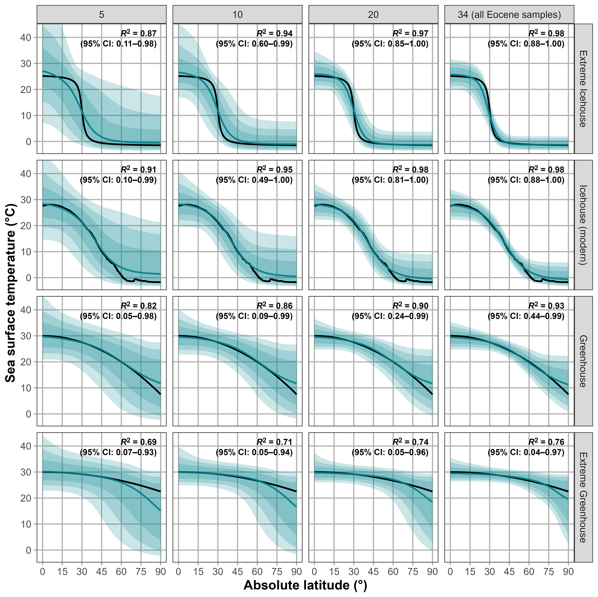
Figure 2 Model reconstructions of simulated latitudinal temperature gradients at various sample sizes. Each column depicts a different reconstruction for given sample sizes: 5, 10, 20 (randomly sampled latitudes), and 34 (latitudes of EECO samples). Each row depicts a different latitudinal temperature gradient that represents idealised or observed climatic states, namely idealised extreme icehouse, greenhouse, and extreme greenhouse gradients, and the modern gradient, which represents an icehouse state. The black line illustrates the original gradient. The blue line depicts the reconstructed gradient represented by the median sea surface temperature value estimated from 1000 model runs with different random samples. To generate the random samples, different random noise from a normal distribution with a standard deviation of 3.8 ^∘C was added to each temperature. The blue shadings depict the 90 %, 95 %, and 99 % credible intervals. Bold black text within each panel depicts the coefficient of determination (R²) for estimating goodness of fit between the simulated and modelled gradient. The median (50 %) R² value, along with the 95 % credible intervals from all model runs, is shown. Each gradient is depicted in absolute latitude.

The average modern temperature gradient can be closely approximated with our model when using the full modern SST dataset (Fig. 3); almost all of the variation in the empirical median temperatures in bins of 1^∘ absolute latitude (black line) is explained by the modelled gradient (99.7 %). The empirical gradient spans 29.3 ^∘C from the Equator to the poles, and the modelled gradient is only slightly higher at 29.6 ^∘C. The modern global mean surface temperature (GMST), based on our modelled median gradient, is 17.6 ^∘C, which is nearly equal to the GMST derived from the empirical median gradient (17.5 ^∘C).

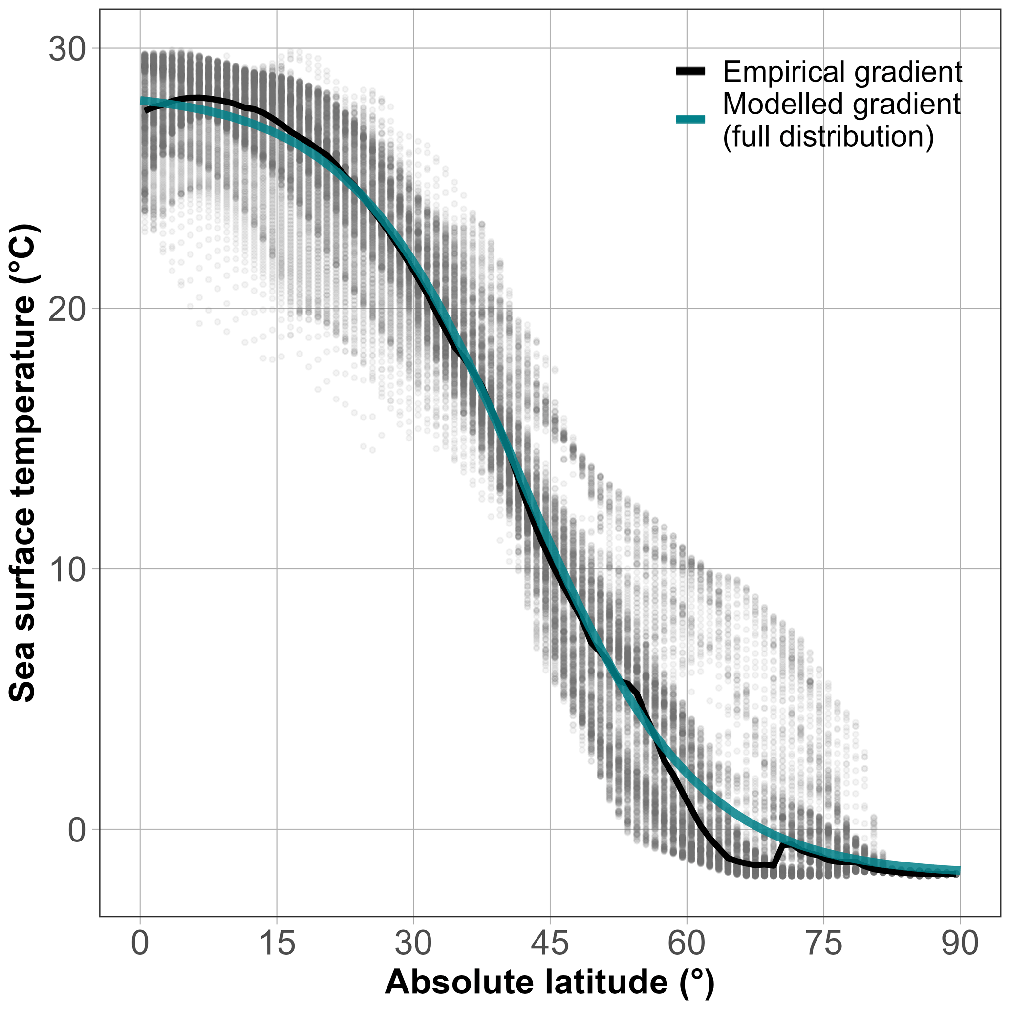
Figure 3 Present-day latitudinal temperature gradient. The present-day empirical latitudinal temperature gradient (median sea surface temperature) is depicted as a black line, and the gradient estimated by the Bayesian model is shown in blue ($R^{\mathrm{2}}=\mathrm{0.97};N=\mathrm{42}\mathrm{896}$). Grey points depict the individual cell values of the Bio-ORACLE grid of mean sea surface temperatures, which were used to infer the empirical and the modelled gradient. Higher opacity of points indicates higher density of data (multiple overlapping points).

3.2 EECO reconstruction

The Eocene temperature gradient reconstructed with our Bayesian model is starkly different from the modern (Fig. 4). Modelled median equatorial temperatures are 2.2 ^∘C (the 95 % CI is −0.8–8.5 ^∘C) higher for the EECO, and polar temperatures are 18.9 ^∘C (5.3–28.9 ^∘C) higher. This results in a flattened latitudinal temperature gradient of 13.3 ^∘C (3.9–25.2 ^∘C) for the EECO, as opposed to 29.6 ^∘C for the modern. To facilitate the comparison with latitudinal gradients reported in the literature, which sometimes does not report temperatures at very high latitudes, we report also the EECO gradient between the Equator and the modern-day polar circle (66.6^∘ latitude), which is markedly lower at 5.8 ^∘C (0.5–12.8 ^∘C).

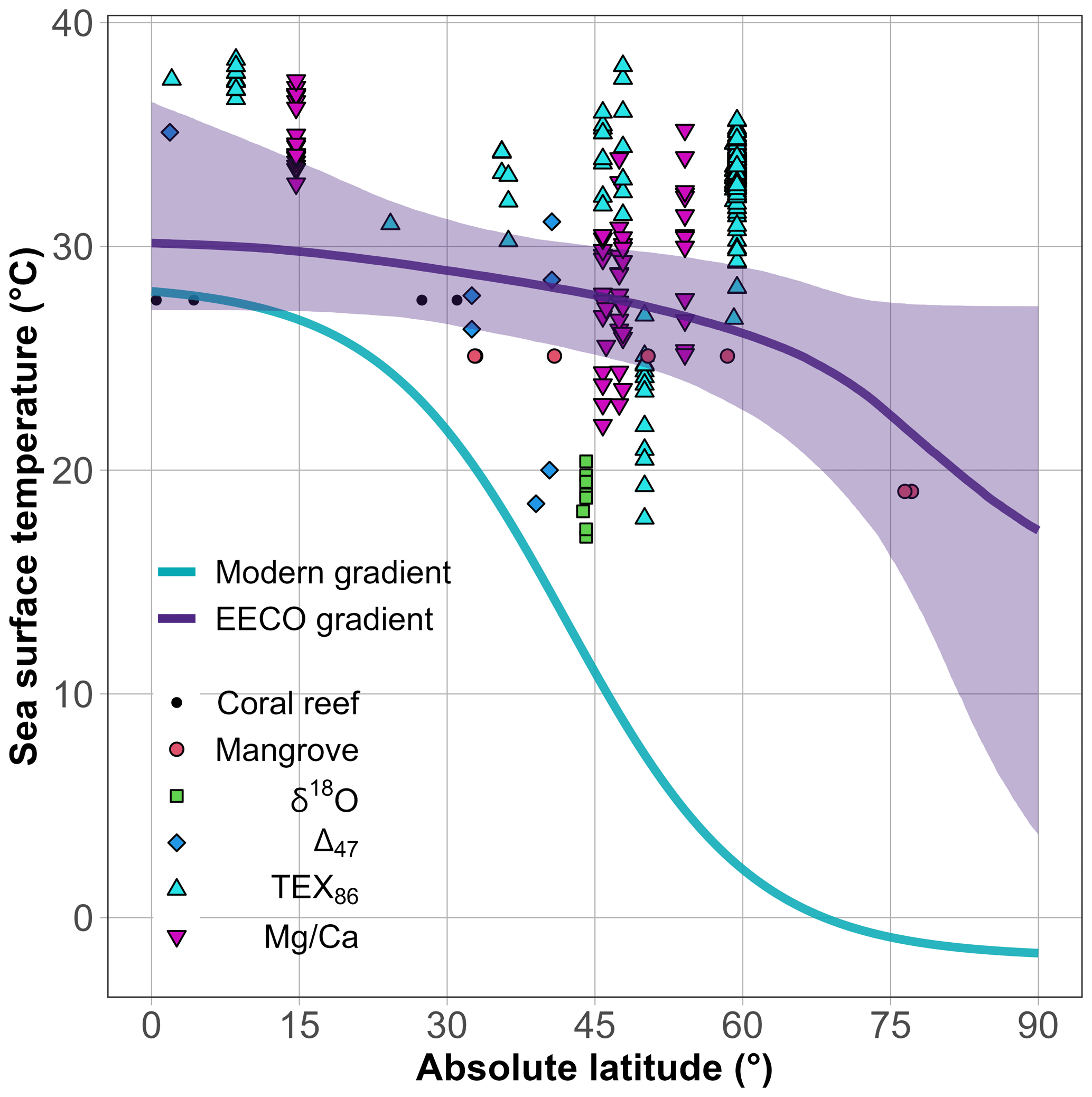
Figure 4 Estimates of the median latitudinal sea surface temperature gradients of the EECO (purple line) and of the present-day (blue), both estimated with the Bayesian model. The purple ribbon (shading) depicts the 95 % credible interval of the Eocene gradient, and the uncertainty about the modern gradient is too low to be visible. Points within the plot depict the geochemical (e.g. TEX₈₆) and the ecological (e.g. mangroves) data. Geochemical data are plotted by their point estimate temperature value. Ecological data are plotted at the mean temperature values of their respective normal distributions.

The high variability in the EECO palaeotemperature proxies, particularly in the mid-latitudes, and the scarcity of high-latitude data, result in substantial uncertainties in the modelled temperature gradient. This is reflected in the residual standard deviation (σ) of the EECO gradient, 4.9 ^∘C (3.9–6.5 ^∘C), which is more than double the σ for the modern gradient, 2.2 ^∘C. This is illustrated by the drastic departure of some of the proxy data from the gradient estimates (Fig. 4).

The early Eocene GMST is estimated at 28.3 ^∘C (26.3–30.3 ^∘C), 10.7 ^∘C higher than the modern. A model run excluding the ecological proxies increases the GMST by 1.7 ^∘C (−1.8–5.0 ^∘C). The median modelled temperature is higher near the Equator and in high latitudes when excluding the ecological proxies, with a flattened median gradient of 10.9 ^∘C (Fig. S2). In contrast, including ecological proxies, but widening the uncertainty around the low-latitude ecological proxy data, does not significantly change the resulting gradient (Fig. S3).

Due to the limited spatial coverage of the early Eocene proxy record, and due to the added model complexity of simultaneously estimating a model across both hemispheres, we pooled the proxy data across both hemispheres. Applying the model separately within each hemisphere results in substantial differences in hemispherical, average temperatures, with the Southern Hemisphere being warmer by 6.1 ^∘C (2.9–9.2 ^∘C). The inferred latitudinal gradient is somewhat steeper in the Northern Hemisphere (steeper by 1.8 ^∘C, although the 95 % CIs of that difference span −18.0–14.5 ^∘C), but the large uncertainties associated with both gradients and the lack of polar proxy data in the Southern Hemisphere preclude a more precise statement (see Fig. S4).

4 Discussion

4.1 Improved estimation of latitudinal and global palaeotemperatures

Our results show that our Bayesian model can be used to reconstruct different types of latitudinal SST gradients from proxy data with moderate sample sizes (n = 10–34) and patchy sampling distributions (Fig. 2). This is an advancement over previously used linear, quadratic, or Gaussian approximations (e.g. Bijl et al., 2009; Tierney et al., 2017), which can fit only specific types of gradients. As such, our model presents an alternative to non-parametric methods for inferring latitudinal temperature gradients, which are sometimes favoured as they can flexibly follow the shape of an unknown temperature gradient (e.g. Zhang et al., 2019; Jones and Eichenseer, 2022). However, when used for interpolation or prediction outside the proxy range, non-parametric methods such as Gaussian process regression strictly respond to the data (e.g. Inglis et al., 2020). This means that the idiosyncrasies of a patchy proxy record, potentially afflicted with measurement errors, calibration errors, and palaeogeographic and temporal uncertainty (e.g. Buffan et al., 2023), dictate the reconstruction of large-scale climatic patterns without the option of including additional knowledge (e.g. that latitudinal temperature gradients should be broadly negative).

In contrast, our Bayesian parametric model allows for the inclusion of informative priors on the model parameters. The modelled sea surface temperature gradient thus does not strictly follow the proxy data but instead represents a compromise between the data and prior knowledge. In the EECO example (Fig. 4), the inclusion of informative priors improves the prediction of sea surface temperatures in the unsampled very high latitudes. Notice that the upper limit of the credible interval does not increase beyond the range of the data, whereas unconstrained approaches such as splines, Gaussian processes, or even standard linear regression could lead to unrealistically high upper bounds in this case (see Rasmussen and Williams, 2004). Prior information on the shape of latitudinal temperature gradients on Earth exists for all geological time periods. For example, the greater amount of solar radiation per unit area in low latitudes causes Earth's latitudinal temperature gradient to be broadly negative (Beer et al., 2008). The ease with which such prior information can be integrated is a major advantage of our method, as the shape of the modelled gradient is controlled by four parameters which clearly relate to its magnitude, steepness, and the latitude of its greatest steepness.

Palaeoclimate reconstructions are often summarised as global mean surface temperatures (GMST), providing a standardised metric for characterising the state of the Earth's climate (Royer et al., 2004; Inglis et al., 2020). The calculation of global mean surface temperatures directly from sparse proxy data is susceptible to bias (Jones and Eichenseer, 2022). By modelling the temperature variation across latitudes, a complete temperature distribution along a latitudinal axis can be obtained, filling in gaps in the proxy record through inter- or extrapolation. This eliminates the common problem that specific climatic zones dominate the proxy record. Reconstructing the GMST directly from the proxies would lead to an estimate biased towards the well-sampled latitudes. Calculating zonal averages alleviates this problem, but this method relies on comprehensive latitudinal coverage (Inglis et al., 2020). Instead, our method allows for intersecting the modelled temperature gradient at narrow latitudinal intervals, even when significant latitudinal gaps exist. Weighting the temperatures of those latitudinal intervals by area results in GMST estimates without intrinsic spatial biases. We anticipate that this improved method may significantly alter Phanerozoic proxy-based temperature curves, which have often been directly calculated from the proxy record (Royer et al., 2004; Veizer and Prokoph, 2015). This is particularly relevant for the early Mesozoic and older intervals, for which the spatial coverage is generally poor due to the absence of data from ocean drilling sites (Jones and Eichenseer, 2022).

4.2 The role of ecological constraints in palaeoclimatic reconstructions

Our results further exemplify how incorporating quantified ecological temperature constraints can provide more precise temperature reconstructions than geochemical proxies alone, adding to the advances in palaeoclimatic reconstructions achieved by integrating lithological data (Scotese et al., 2021; Burgener et al., 2023). Combining the occurrences of climate-sensitive plant communities (Greenwood and Wing, 1995), reptiles (Markwick, 2007), and leaf shapes (Peppe et al., 2011) with geochemical proxies offers substantial potential for improving quantitative palaeoclimatic reconstructions across the Phanerozoic. Our modelling framework offers a straightforward, efficient way of integrating ecological palaeoclimatic data with other proxy data. The hierarchical model structure accounts for variation in the temperature estimates from proxies at individual localities, which is treated equivalent to the uncertainty associated with the ecological temperature proxies. A local temperature estimate, based on multiple geochemical proxies, thus has the same weight as a local temperature estimate obtained from the occurrence of a climate-sensitive plant community, while preserving the uncertainty associated with each estimate. The model could easily be extended to include uncertainties about individual geochemical proxy data (see Fig. S5) or to variably weight proxy records classified as more or less reliable.

Our approach for deriving fully quantitative climate reconstructions from ecological data is borrowed from nearest-living-relative methods commonly employed in terrestrial Cenozoic palaeoclimatic reconstructions (Fauquette et al., 2007; Pross et al., 2012). One major limitation to these methods is that the thermal preferences of taxa may have changed over time. More significantly, in the early Eocene, sea surface temperatures may have reached heights unknown in the modern world, and nearest living relative methods based on the modern are inherently unable to predict such elevated temperatures. This is especially true for taxa that inhabit the warmest part of the ocean today, e.g. coral reefs (Kleypas et al., 1999). Although coral reefs are threatened by warming sea surface temperatures today (Hoegh-Guldberg, 2011), it is conceivable that Eocene reef corals were adapted to a warmer climate. The fossil record indicates that reef development may have been stunted in the early Eocene, with few early Eocene coral reefs occurring in low latitudes (Zamagni et al., 2012). The absence of coral reefs in higher latitudes in the early Eocene could be due to requirements in irradiance rather than temperature (Muir et al., 2015). Tropical temperatures predicted by the geochemical proxy record indicate hotter-than-modern tropical temperatures for the early Eocene (Fig. S2), suggesting that the modern climatic range of coral reefs may underestimate the early Eocene thermal limits for coral reefs. We have tried to account for that possibility by widening the temperature probability distribution for coral reefs, but the predicted temperatures for the reef and mangrove sites still lie below the temperatures indicated by the geochemical proxy record (Figs. 4 and S2).

4.3 Early Eocene climate

The geochemical proxy record and ecological data indicate that the latitudinal SST gradient of the EECO was significantly shallower than the modern (Huber and Caballero, 2011), but beyond that, there is little agreement. Earlier reconstructed early Eocene and EECO SST gradients range from 7–21 ^∘C (Table 1); a more recent reconstruction that includes terrestrial air and sea surface temperatures arrives at a gradient of ∼ 13 ^∘C (Inglis et al., 2020). Our median poles-to-Equator gradient estimate is similar at 13.3 ^∘C but notably shallower when taking the Equator-to-polar-circle estimate, 5.8 ^∘C, as the geochemical proxy data suggest high temperatures up to latitudes of ∼ 60^∘. Both geochemical and ecological shallow-water data indicate that inferred SST gradients based on tropical shallow-water and deepwater samples (Cramwinckel et al., 2018; Evans et al., 2018) may overestimate the SST gradient of the early Eocene greenhouse world. Likewise, palaeoclimatic simulations from General Circulation Models tend to estimate steeper gradients than most proxy records (Table 1; Pross et al., 2012; Lunt et al., 2021)

The very high variability in the proxy record in mid-latitudes results in large uncertainties about the shape of temperature gradient and on the GMST. Some of this variability may stem from spatial variability in SSTs, as can be observed in the modern (Fig. 3), e.g. due to ocean circulation (Rahmstorf, 2002). Biases and errors in the proxy reconstructions also likely contribute to the observed variability, as geochemical proxies reflect many other factors besides seawater temperature (Hollis et al., 2019). Despite excluding δ¹⁸O measurements from recrystallised fossils, systematic offsets remain between mostly warm temperatures derived from TEX₈₆ and cooler temperatures derived from δ¹⁸O, Δ₄₇, and the ecological proxies.

Temporal changes within the EECO (Westerhold et al., 2018) and seasonality (Keating-Bitonti et al., 2011; Ivany and Judd, 2022) may also contribute to the large variability in the EECO proxy data. Based on the occurrence of heterotrophic carbonates, Davies et al. (2019) suggested that mid- and high-latitude geochemical proxy data from the EECO may be biased towards summer temperatures. Some of the geochemical mid-latitude geochemical proxy data from Hollis et al. (2019) may therefore suggest higher than actual mean annual temperatures, and the variability in the temperature estimates from individual localities is higher in mid–high latitudes (Fig. S6). It is difficult to attribute this variability to seasonality alone, as temporal climate variability is also expected to be higher in mid and high latitudes (Schwartz, 2008). Critically, however, the mangrove data strongly support our inference of a flattened gradient independent of the geochemical proxy record.

Recent marine GMST estimates of the EECO and of the early Eocene range from 23.4–37.1 ^∘C, with the lowest GMSTs being derived from δ¹⁸O, and the higher estimates including TEX₈₆ (Inglis et al., 2020). Many studies include both marine and terrestrial proxies to derive GMST estimates, but despite great differences in proxy selection and in the calculation of global average temperatures, many recent estimates fall in the range of 27–29.5 ^∘C (Hansen et al., 2013; Caballero and Huber, 2013; Cramwinckel et al., 2018; Zhu et al., 2019), similar to our median GMST estimate of 28.3 ^∘C and well within the 95 % credible intervals of our GMST estimate (26.3–30.3 ^∘C).

5 Conclusions

The Bayesian hierarchical model presented here is able to reconstruct latitudinal gradients from both geochemical and ecological proxy data, while reflecting the uncertainty associated with the ecological temperature proxies and accounting for the variation in the multiple temperature estimates at individual localities. Using informative prior information allows for accurate temperature reconstructions from records with geographically sparse sampling. By providing temperature estimates across the entire latitudinal range, this method also facilitates the reconstruction of unbiased global average temperatures. Application of our model to the EECO suggests that latitudinal sea surface temperature gradients were shallower than estimated by most previous proxy-based studies. High-latitude pollen records support this interpretation. Our GMST estimate is in good agreement with most existing estimates, indicating that broadly accurate GMST reconstructions are possible even with substantial deviations in the shape of the latitudinal temperature gradient. Our new method opens the door for improving the accuracy of proxy-based palaeoclimatic reconstructions and Phanerozoic temperature curves, particularly in intervals with a patchy and unevenly sampled record. Finally, the flexibility of our approach means that estimates can be efficiently updated when new data, or constraints, are made available.