the Creative Commons Attribution 4.0 License.
the Creative Commons Attribution 4.0 License.
 | 12 Sep 2024
Can we reliably reconstruct the mid-Pliocene Warm Period with sparse data and uncertain models?
James D. Annan
Julia C. Hargreaves
Thorsten Mauritsen
Erin McClymont
Sze Ling Ho
We present a reconstruction of the surface climate of the mid-Pliocene Warm Period (mPWP), specifically Marine Isotope Stage (MIS) KM5c or 3.205 Ma. We combine the ensemble of climate model simulations, which contributed to the Pliocene Model Intercomparison Project (PlioMIP), with compilations of proxy data analyses of sea surface temperature (SST). The different data sets we considered are all sparse with high uncertainty, and the best estimate of annual global mean surface air temperature (SAT) anomaly varies from 2.1 up to 4.8 °C depending on the data source.
We argue that the latest PlioVAR analysis of alkenone data is likely more reliable than other data sets we consider, and using this data set yields an SAT anomaly of 3.9±1.1 °C, with a value of 2.8±0.9 °C for SST (all uncertainties are quoted at 1 standard deviation). However, depending on the application, it may be advisable to consider the broader range arising from the various data sets to account for structural uncertainty. The regional-scale information in the reconstruction may not be reliable as it is largely based on the patterns simulated by the models.
- Article
(5593 KB) - Full-text XML
- BibTeX
- EndNote


The mid-Pliocene Warm Period (mPWP; also mid-Piacenzian Warm Period), roughly 3.2 Ma, represents the most recent period when atmospheric CO2 was significantly higher than the pre-industrial level for a sustained period and, as such, is an attractive target for analysis in order to better understand how our modern climate system may respond to sustained elevated greenhouse gas concentrations. It has been the focus of two international climate modelling projects, Pliocene Model Intercomparison Project Phase 1 (PlioMIP1) (Haywood et al., 2010) and Pliocene Model Intercomparison Project Phase 2 (PlioMIP2) (Haywood et al., 2016), in each of which a common protocol was developed in order that multiple climate models from different research centres could generate simulations which may be compared to each other and also to proxy data collected and analysed from this time interval.
While models provide global fields that attempt to represent the climate state at that time, these outputs do not directly use surface temperature information from proxy data, and their representation of the physics of the climate system is imperfect. There have been few attempts to estimate the climate state (e.g. global temperature fields) based on proxy data, and these have generally used statistical approaches which do not take advantage of the physical constraints represented by climate models. For example, Bragg (2014) generated a surface temperature reconstruction based on a Gaussian Markov random field using the earlier PRISM3 data, but this method does not account for physical properties of the climate system, such as land–sea contrast or polar amplification, which are underpinned by physical theory and robustly reproduced in models. When data are sparse and uncertain, as is the case here, it is necessary to interpolate to unobserved regions. Inglis et al. (2020) compared numerous heuristic and statistical methods to generate global mean temperature estimates for periods considered in the DeepMIP project (which did not include the mPWP). Data assimilation methods, which combine the physics embedded in climate models with the sparse and uncertain observations that are available, have the potential to improve on methods that rely on either models or data alone.
In Annan and Hargreaves (2013), we presented a novel approach to reconstructing the surface temperature fields (both surface air temperature, or SAT, and sea surface temperature, or SST) for the Last Glacial Maximum (LGM; 19–23 ka) which combined the “ensemble of opportunity” of model simulations of this time period with compilations of proxy-based surface temperature estimates. The inputs and methods were updated in Annan et al. (2022) (henceforth AHM22). Here we apply the same method as that presented in AHM22 to reconstruct the surface temperature fields of the mPWP, specifically Marine Isotope Stage (MIS) KM5c or 3.205 Ma. We combine the ensemble of climate model simulations, which contributed to the PlioMIP projects, with compilations of SST proxy data to provide an estimate of the climate state at the mPWP. We introduce the model ensemble in Sect. 2. Two compilations of proxy data relating to this period have been published by Foley and Dowsett (2019) and McClymont et al. (2020), which we discuss further in Sect. 3. We discuss methodological choices and their impact in Sect. 4 and summarize our results in Sect. 5.
There are two major modelling projects focusing on the mPWP. The first Pliocene Model Intercomparison Project (Haywood et al., 2010), which we refer to as PlioMIP1 for clarity, comprised nine models simulating a generic interglacial period in the range of 3.264 to 3.025 Ma BP. For the second Pliocene Model Intercomparison Project, or PlioMIP2 (Haywood et al., 2016), the specific interglacial period MIS KM5c was simulated, dated at 3.205 Ma BP. The boundary conditions thus varied slightly between the two projects, but the importance of these differences in determining the outputs of the simulations is small compared to the differences in physics between the models. Thus, as our initial ensemble, we take the results of all the model simulations from both projects.
There are 9 simulations available from PlioMIP1 and 16 from PlioMIP2, with the models listed in Table 1. In order to perform our synthesis, model outputs were interpolated onto a regular 2×2° grid for SAT and a 5×5° grid for SST. The ocean boundary varies slightly between models due to various differences in resolution and underlying model grid. Our algorithm requires all ensemble members to generate output at each grid point; thus we mask out all locations on the SST grid where any model has land. While this has the unfortunate effect of reducing the number of usable data points, we note that the points that are masked in this way are coastal in location, which is potentially problematic for data–model comparisons due to the local nature of upwelling dynamics that is not always adequately captured by models.
Table 1Models available for the mPWP reconstruction and their global mean surface air temperature anomalies for the mPWP. Parentheses indicate models which were removed due to similarity. See text for details.
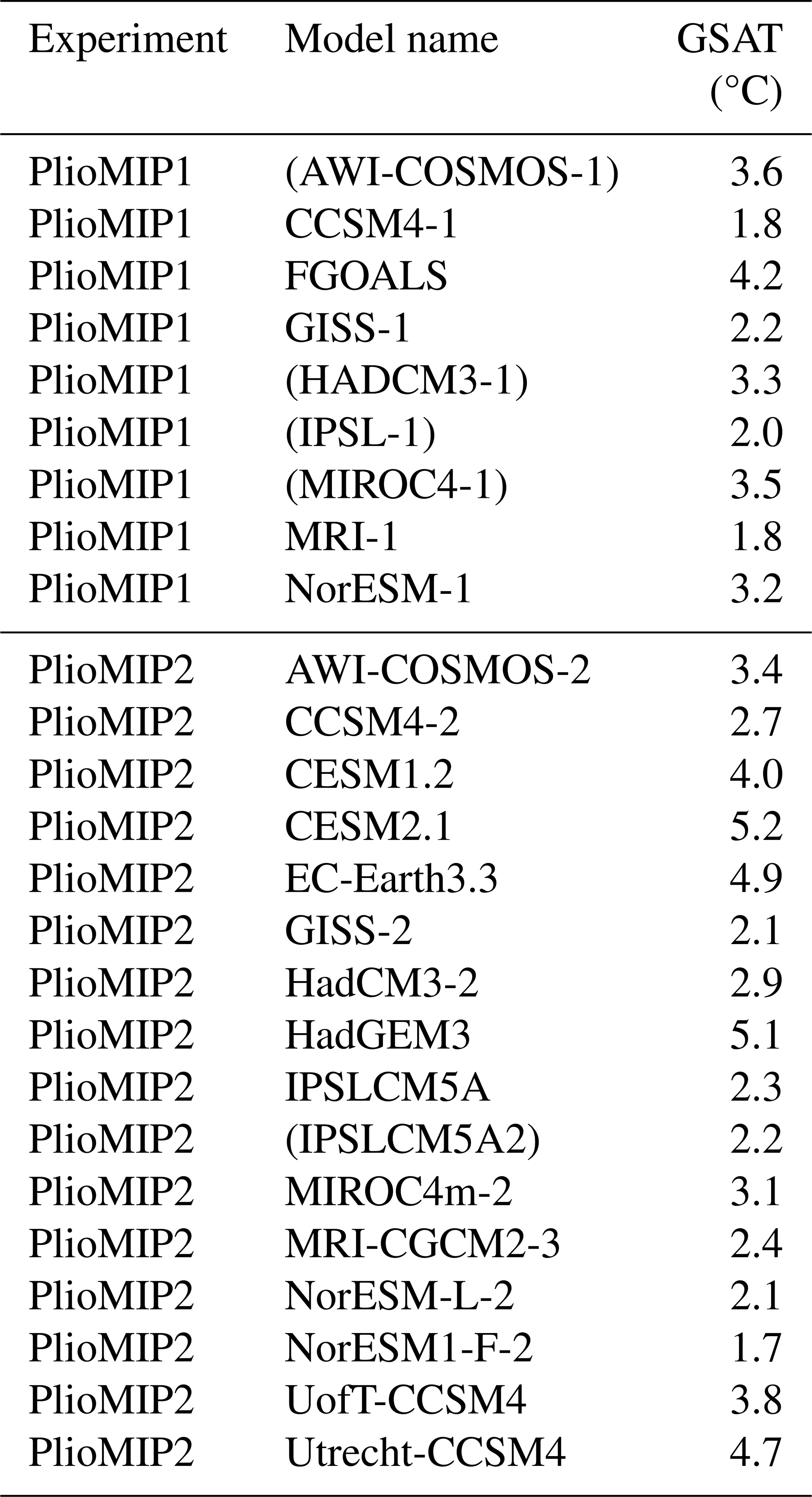
As Table 1 indicates, some models either directly contributed more than one simulation to the combined ensemble or else were closely related to other models that participated. Therefore we performed a thinning process similar to that described in AHM22. The goal is to generate an ensemble where we do not expect to find any clustering where particular sets of models have highly similar outputs. We examined the literature to consider which models were closely related through their construction to other models in the ensemble. Then we checked this assessment by calculating root mean square (rms) differences and correlations between the simulated anomalies. We concluded that the following subsets of models were too similar for them to contribute more than one member to our ensemble: (AWI-COSMOS-1, AWI-COSMOS-2), (HADCM3-1, HadCM3-2), (IPSL-1, IPSLCM5A1, IPSLCM5A2), and (MIROC4-1, MIROC4m-2). From these, we removed the models as indicated in the table, retaining the newest of each set, leaving us with a final ensemble of 20 model simulations. The set of global mean SAT values from this ensemble (3.2±1.2 °C at 1 standard deviation) passed a Shapiro–Wilk test of normality.
The ensemble mean surface temperature anomaly fields for this 20-member ensemble are shown in Fig. 1 along with other results that we will discuss later. The extent of our land mask is shown in the SST plots. The location and values of one set of data points are also indicated on the SST field, and we discuss these in the following section.
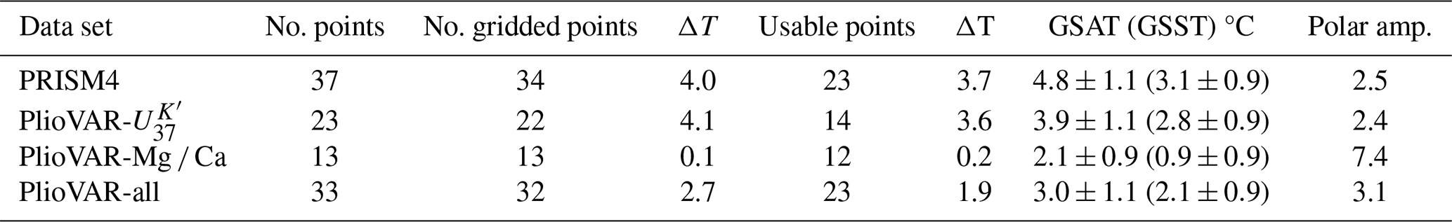
We consider various data sets in this paper, all of which have been calibrated to SST. The most widely used data sets for analysis and interpretation of the mPWP are those generated by various iterations of the PRISM projects (Foley and Dowsett, 2019). Here we primarily consider the PRISM4 proxy estimates for SST from a 30 ka wide interval centred on MIS KM5c (Foley and Dowsett, 2019), which is 3.205±0.015 Ma. We also consider their SST estimates based on data limited to the more restricted interval of 3.205±0.005 Ma, but the differences between these two analyses are very minor. PRISM4 SSTs were compiled from published literature using an alkenone SST proxy (the index), which is converted to mean annual SST using a linear calibration based on globally distributed surface sediment data (Müller et al., 1998). Anomalies from the pre-industrial climate are calculated relative to the NOAA ERSSTv5 data set (Huang et al., 2017). This PRISM4 compilation contains 37 data points, reducing to 34 distinct grid points on the regular 5×5° grid that we use for our SST analysis, of which 23 locations remain after masking to the ocean grid of our ensemble. The tighter 3.205±0.005 Ma compilation of PRISM4 data contained only 33 points, but these still covered the same 23 grid points on the ocean grid of our ensemble. No uncertainty estimates were included with these data. We assume a value of 2 °C for the uncertainty at 1 standard deviation, which is larger than the value of 1 °C that we used for various proxy estimates when reconstructing the Last Glacial Maximum (Annan and Hargreaves, 2013) but may still be optimistic, given there is generally less certainty for older palaeo-periods. We discuss this choice in Sect. 4.
More recently, the PlioVAR project (McClymont et al., 2020) produced an updated analysis of proxy data to examine the 20 ka wide interval of 3.205±0.01 Ma. The PlioVAR project required data to have a minimum temporal resolution (≤10 kyr) and be constrained in time by an orbital-scale age model. Several PRISM4 sites were excluded as a result of this strict stratigraphic protocol, and for others there was a revision to the original published age model where the MIS KM5c peak had been misaligned (McClymont et al., 2020). Within the PlioVAR data set we consider separately the data points, of which there are 23, and the Mg Ca data points of which there are 13.
For the data, two SST calibrations were available and compared by PlioVAR: the linear Müller et al. (1998) calibration and a more recent Bayesian calibration (Tierney and Tingley, 2018). At high and mid-latitudes the reconstructed SSTs differ by less than 1 °C, whereas in the equatorial region the difference may be up to 1.5 °C (McClymont et al., 2020), which is smaller than the individual calibration errors. The SST values we take here are the simple average of the calibration of Müller et al. (1998) and the BAYSPLINE calculation, as presented in McClymont et al. (2020).
In McClymont et al. (2020), the Mg Ca SST values presented were unaltered from the original estimates in the source publications. Subsequently, the calibrations were revisited, and consistent corrections were applied, including for evolving seawater Mg Ca and potential dissolution (McClymont et al., 2023). This updated data set also includes one data point based on the organic proxy “TEX86” (Schouten et al., 2002), which we include within the Mg Ca data set for convenience. For Mg Ca, we use the newer values where available and the calibration presented in McClymont et al. (2020) for the remainder. We discard the Mg Ca SST estimates generated by a Bayesian calibration (BAYMAG), which were also presented in McClymont et al. (2020), although we have checked that including these does not qualitatively change our analysis, as we describe further below. The data values that we use here are made available along with the calculation code in order to ensure reproducibility.
In cases where multiple data points from the same proxy type coincide on the grid, we use simple averages. In the case where both Mg Ca and data coincide in the same box, we then average their averages, thereby giving equal weight to the Mg Ca and the . We refer to the data sets thus derived as PlioVAR-, PlioVAR-Mg Ca, and PlioVAR-all. The locations and values of the data sets used can be seen in the SST plots of Fig. 1. As for the PRISM4 data, uncertainties of 2 °C are assumed for the final gridded and averaged values.
The PRISM4 and PlioVAR data sets overlap substantially in locations. This is unsurprising, since they are based on largely the same set of drilled cores. There are 17 grid points in common between PRISM4 and PlioVAR-, and the values at these locations are highly consistent, matching well with a mean difference of 0.0 °C and an rms difference of 0.7 °C. The correlation of the two data sets at these coincident locations is also very high at 0.97. While the new PlioVAR chronology and recalibration have introduced changes in SST values at the grid-point level, these have broadly cancelled out overall. McClymont et al. (2020) highlighted some inconsistencies between the Mg Ca data and both the data and the PlioMIP models. There are six locations in common between the PRISM4 and PlioVAR-Mg Ca data sets, and these also have a very substantial mean difference of 3.3 °C (PlioVAR-Mg Ca being cooler), with a residual rms of 5.1 °C. It does not seem possible that both data sets are faithful representations of the annual mean sea surface temperature that is required for our analysis. As discussed extensively in previous studies (e.g. De Schepper et al., 2013; Dekens et al., 2008; Evans et al., 2016; Karas et al., 2020; Lawrence and Woodard, 2017; Leduc et al., 2014; Naafs et al., 2020), the relationship between Mg Ca and annual mean SST may depend on a range of site-specific factors, including the species analysed, the calibration used, and the seasonality or depth habitat of the foraminifera. Therefore, since our focus here is on the determination of the annual surface temperature signal recorded by the proxies, we regard the Mg Ca ratio as having a more complex relationship to SST than the data (e.g. McClymont et al., 2023)
The Mg Ca data set might be regarded as less reliable as its relationship to SST may depend on site-specific factors, including the species analysed, the calibration used, and the seasonality or depth habitat of the foraminifera.
Of the three data sets, PlioVAR- shows the closest agreement with the models, with a pointwise rms difference of 2.2° C from the ensemble mean, whereas the PlioVAR-Mg Ca and PRISM4 data sets differ from the ensemble mean by almost 3 and 4 °C respectively. This latter figure may seem surprising since the PlioVAR- and PRISM4 data agree rather well where both data sets coincide, but apparently the PRISM4 cores that are not included in the PlioVAR- data set show a markedly greater divergence from the models.
Our preferred reconstruction is thus based on the PlioVAR- data set, but we also calculate reconstructions using the other data sets to explore the low level of agreement between proxies, and it may be advisable to use the full range of results we present in order to account for the uncertainties in the proxy data analysis. The locations and values of the alternative SST data sets used can be seen in the SST plots of Fig. 4. All four data sets, and the climate reconstructions they generate, are summarized in Table 2.
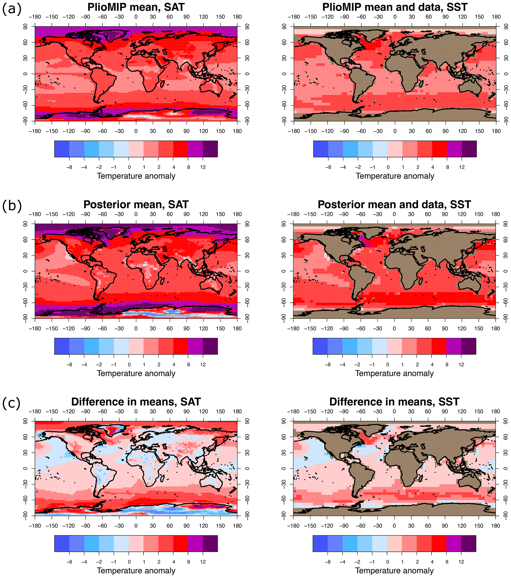
Figure 1Initial PlioMIP ensemble mean and results obtained using the PlioVAR- data set. (a) PlioMIP ensemble means, SAT and SST (with proxy data). (b) Posterior means, SAT and SST (with proxy data). (c) Difference between final reconstruction and PlioMIP ensemble means (location of proxy data points shown).
Table 2Summary of data sets and main results. Columns show the number of points in the data set, the number of points in the 5° grid, the average temperature of the data points, the annual mean global air (sea) temperature from the climate reconstruction using the data set, and the polar amplification of the reconstruction. All uncertainties are quoted at 1 standard deviation.
While there are some proxy data relating to the land surface (Salzmann et al., 2008, 2013), the dating and precision in terms of inferred temperature do not yet appear to be sufficiently robust for us to use here. Multiple proxies covering land and ocean would enable more precise and robust climate reconstructions, and we expect that the analysis presented here may be improved in future years.
The method follows that of AHM22. That is, we firstly perform a re-centring step to shift the ensemble mean towards the data. This is done through a pattern scaling approach in which we fit the first four empirical orthogonal functions (EOFs) of the ensemble to the data points and take this result as our ensemble mean. Our justification for this step, as in AHM22, is that we do not regard the PlioMIP ensemble of opportunity as a reliable prior, since the models may share common biases in both their physics and the boundary conditions that are applied. With this re-centring procedure, AHM22 demonstrated that we can strongly reduce the influence of possible biases in the model ensemble on the posterior. Some evidence for this is shown in the rank histograms of Fig. 2, the left panel of which compares the data points to the original PlioMIP ensemble. With so few data points, the evidence of a bias between models and data is not compelling, but a large majority of points lie in the right-hand side of the rank histogram, with 6 of the 14 points in the top quarter. Re-centring the prior leads to a more even distribution of data points across the ensemble, as shown in the right panel of Fig. 2. Ideally, the rank histogram should be flat with a uniform spread of data points. The re-centring step does not alter the covariance structure of the ensemble, merely shifting the mean. We then perform a standard ensemble Kalman filter (EnKF) assimilation step using the proxy data in a similar manner to that of AHM22 and Tierney et al. (2020).
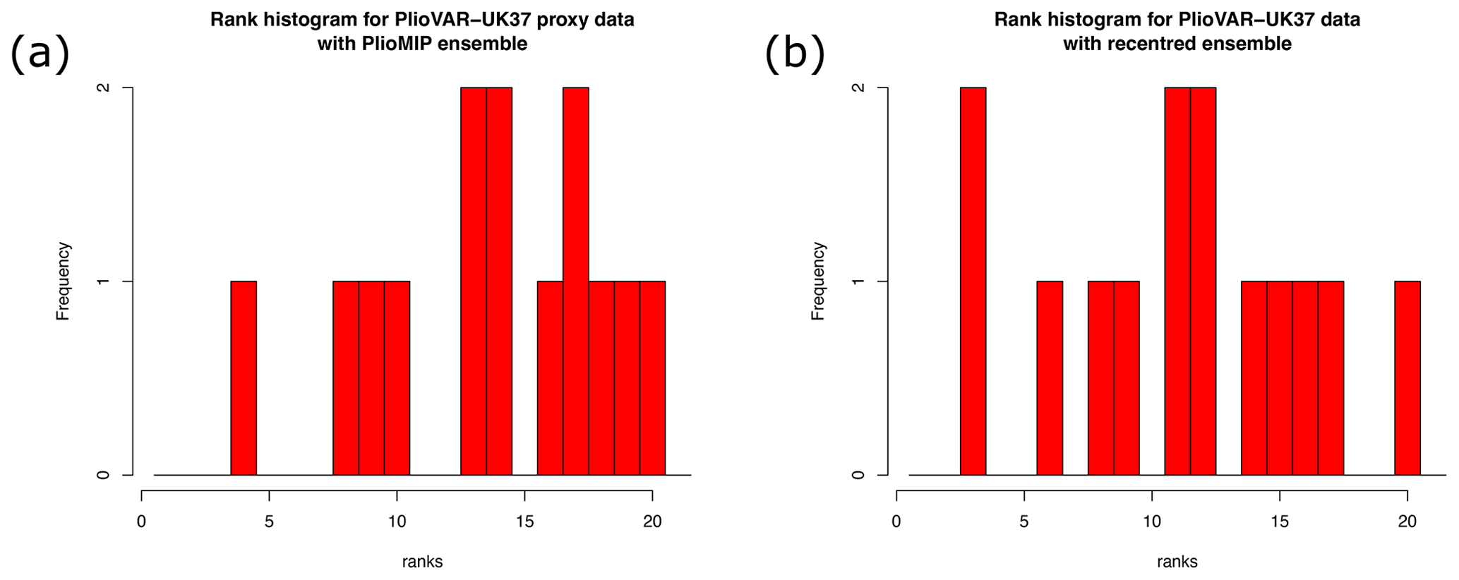
Figure 2Rank histograms of PlioVAR- data in (a) the original PlioMIP ensemble and (b) the re-centred ensemble.
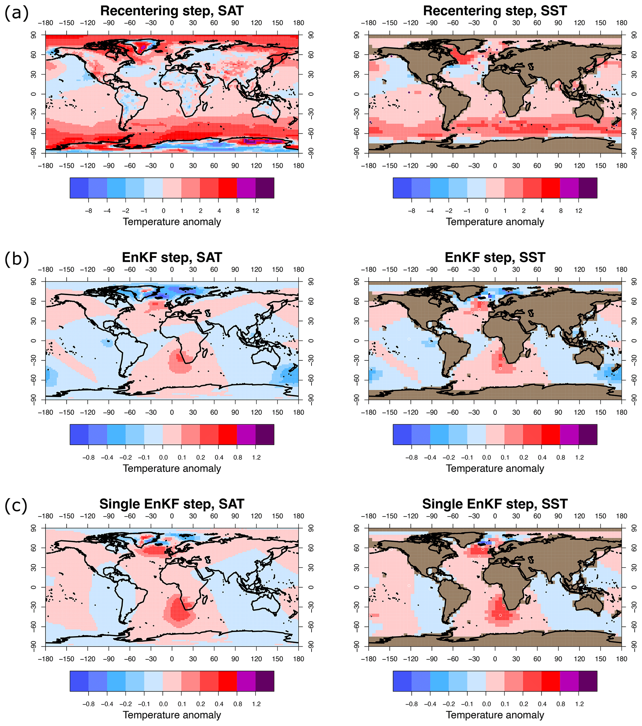
Figure 3Comparison of the two-step (re-centring and EnKF) versus single-step (EnKF only) process. Panels (a) and (b) show the increments generated in the re-centring step and EnKF step respectively in the two-step process using PlioVAR-. Panel (c) shows the increment generated in a single-step EnKF procedure. Note the different scale on the colour bar for the EnKF steps.
Unlike the reconstruction of the Last Glacial Maximum described in AHM22, however, the re-centring step here has a striking influence on the final result. This is simply because the data lie some way from the ensemble mean, being generally warmer, as the rank histograms indicate. If we believed that our model ensemble was a good prior, then it would be appropriate to omit the re-centring step and perform the assimilation directly on the PlioMIP ensemble. However, the EnKF assimilation only updates the ensemble in the neighbourhood of data points (due to both the generally local nature of the empirical correlations in the ensemble and the imposed localization) and therefore cannot interpolate far into data-void regions. Thus, our final result would be highly dependent on the model prior. To illustrate the effect of our methodological choices, here we compare our two-step results with this alternative framework. Figure 3 compares our two-step process with the single-step EnKF approach using the PlioMIP models as a prior without the re-centring step. The top two pairs of panels show the magnitude of change in the ensemble mean, first from centring the ensemble on the data (via the EOF pattern scaling as described in AHM22) and then from applying the EnKF algorithm to this ensemble. Note the factor-of-10 change in scaling on the colour bars between the plots of the re-centring and the EnKF steps. The EnKF update generates changes only in the vicinity of the data points, due to both the localization which was imposed (a length parameter of 2500 km in the Gaspari and Cohn (1999) scheme was used here, as in AHM22, corresponding to a cut-off radius of 5000 km) and the typically local nature of covariances across the ensemble. The changes are small even at the data locations due to the low density of data points and the large uncertainties assumed for these proxy data. If we were to assume a lower uncertainty in these points, then the update would be somewhat larger but would still be limited to the neighbourhood of the data points.
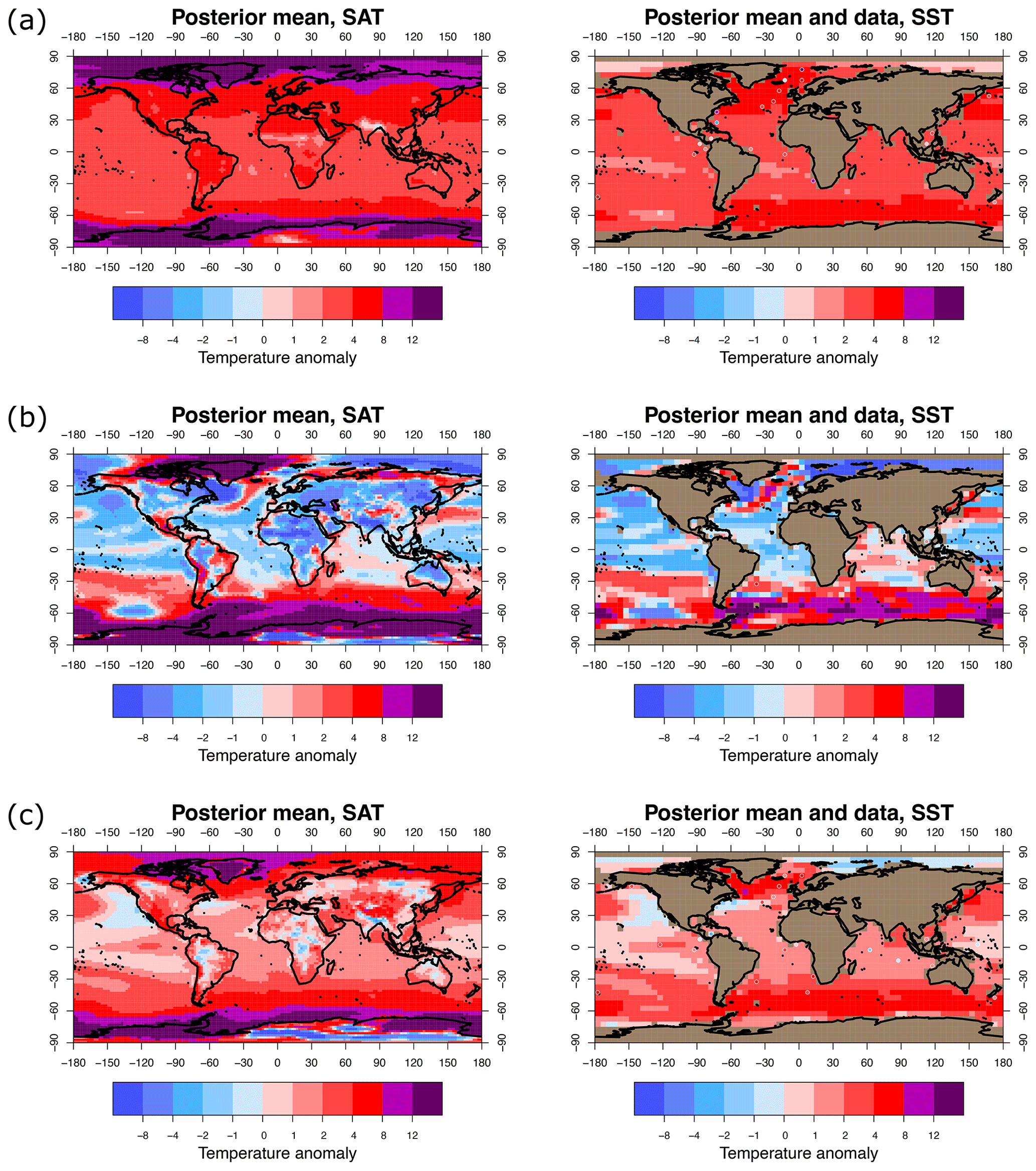
Figure 4Results using three different data sets. (a) Posterior means using PRISM4 data. (b) Posterior means using PlioVAR-Mg Ca data. (c) Posterior means using PlioVAR-all data.
If we do not perform the re-centring and instead just perform the single-step standard EnKF update to the original PlioMIP ensemble, the update is slightly greater than the EnKF step in the two-step method and generally more positive due to the data being warmer than the ensemble mean. However, the increment is still small, as the data are sparse and uncertain. Large areas of the globe are almost unaffected by the assimilation, with a temperature change of less than 0.1 °C. This is an inevitable consequence of having limited sparse data, and it points to the influence of the model prior on the final result. Thus, with so few and uncertain data points, the final result using a one-step framework would be very heavily based on the initial ensemble. This result is very different from that of AHM22, where the re-centring step had relatively small influence on the final result, and the much larger data set of around 400 data points, scattered across both land and ocean, meant that the EnKF update step was more substantial. When the re-centring step is omitted, data cannot possibly influence the posterior beyond the cut-off radius; therefore we also tested the analysis with larger length parameters of up to 10 000 km (corresponding to a cut-off radius of 20 000 km). However, our results were unchanged to within rounding error, demonstrating that the choice of length scale was not a significant factor in our results.
We take a uniform uncertainty of 2 °C for all of our data points. With so few data points, the estimate itself is necessarily uncertain, but we regard it as reasonable for the following arguments. The rms difference between the original PlioMIP ensemble members and the data points is around 2.6 °C averaged across the ensemble members, or 2.2 °C relative to the ensemble mean, which precludes a much higher error value since the data should not be closer to the models than they are to reality under the assumption that model errors and data errors are independent. Conversely, our posterior mean estimate after fitting to the data only achieves a residual rms difference of 1.7 °C. While we could hope that the data uncertainties are smaller than those we have achieved, we note that the rms difference between the PRISM4 data and the Mg Ca data is greater than 5 °C (at the six coincident points), which is a worrying indication that the calibration to SST may not be adequately understood at this point. In Sect. 3 we argued that the Mg Ca data may be less reliable. We do not explore possible reasons for this here, but they may include site-specific factors, such as the species analysed, the calibration used, and the seasonality or depth habitat of the foraminifera (e.g. McClymont et al., 2023, and references therein).
We adopt the same parameters for the algorithm that were shown to work well in AHM22: four EOFs and a localization length parameter of 2500 km, implying a cut-off radius of 5000 km. While changing these values altered the regional patterns somewhat (for example, using a larger number of EOFs introduced more spatial variability), they made little difference to the large-scale results, such as global mean temperature anomalies. In AHM22, we performed extensive validation of the method and the choice of parameters through a process of leave-one-out cross-validation. Here, however, we have so few data points that this process cannot be useful, as the sampling error on the statistics will be much larger than any realistic estimate of the underlying effects being investigated.
5.1 Mean state
We create climate state reconstructions using the filtered PlioMIP model ensemble described in Sect. 2, together with four different data sets. The data sets we use are PRISM4, PlioVAR-, PlioVAR-Mg Ca, and PlioVAR-all, as described in Sect. 3. The global mean temperature estimates obtained are shown in Table 2.
We find that the PRISM4 and PlioVAR- data sets both generate reconstructions towards the high end of previous estimates but are not inconsistent with them (e.g. the value of 3±1 °C assessed by Sherwood et al., 2020). As the table shows, there are differences between the global fields generated from PRISM4 and PlioVAR- data even though the data points in these two sets take broadly similar values where they exist in both sets of data. In contrast, the PlioVAR-Mg Ca data generate a strikingly cooler result, and the inclusion of these Mg Ca data in PlioVAR-all generates a result with considerably less warming than for PRISM4 and PlioVAR-UK37. The reason for these results is simply that the Mg Ca data themselves indicate very little warming and even a cooling in the tropics (McClymont et al., 2020).
Due to the updated chronology and more robust calibration using two approaches, we expect that the PlioVAR- data are likely to be more reliable than PRISM4; therefore we take as our primary reconstruction the PlioVAR- result with global annually averaged SAT (SST) of 3.9±1.1 (2.8±0.9) °C. In comparison, the original 20-member PlioMIP ensemble (that is, after deletion of near-duplicates) has a global mean SAT anomaly distribution of 3.2±1.2 °C. The middle plots in Fig. 1 show the fields obtained by using the PlioVAR- data, while the lower plots on the same figure show the difference between these results and the original PlioMIP ensemble mean. For completeness, the SAT and SST fields obtained from the other three data sets are shown in Fig. 4.
5.2 Polar amplification
Following Haywood et al. (2020), we use as our definition of polar amplification the ratio of warming poleward of 60° in both hemispheres to the global mean change (Smith et al., 2019). The polar amplification in our combined PlioMIP ensemble mean is 2.3, the same as that found by Haywood et al. (2020), increasing slightly to 2.5 in the posterior when using PRISM4 and 2.4 when using PlioVAR-. Much larger polar amplification is obtained when the Mg Ca data are included, due to the greatly reduced tropical warming. We have low confidence in regional results due to the limited and imprecise nature of the data.
We have made the first combined air and sea temperature field reconstructions for the mid-Pliocene Warm Period, using various available data sets and a 20-member model ensemble. For the data set in which we have most confidence (PlioVAR-), our result for annual average global mean surface air (sea) temperatures is 3.9±1.1 (2.8±0.9) K. However, the different data sets produce rather different estimates ranging from 2.1 to 4.8 °C for the best estimate of global surface air temperature anomaly. All the data sets are sparse with high uncertainty; therefore our confidence in our result is not very high. We think that the regional-scale information in the reconstruction is not likely to be reliable as it mostly arises during the re-centring procedure, which simply re-scales the model patterns including in regions where there are no data. A larger data set would improve this.
With such small data sets as we have here, the models also necessarily play an uncomfortably large role. In all of our experiments, the assimilation step of the ensemble Kalman filter makes a relatively small change to the prior. We have investigated the effect of using the original PlioMIP models themselves as a prior versus re-centring the ensemble on the data. This choice has a much more significant influence on the results. In principle, we prefer the data-centred approach because the models could easily be biased through poorly modelled physical processes or uncertainties in boundary conditions, but this is not an unquestionable choice to make. The issue is simply that the data typically available for reconstructions of palaeoclimates are insufficient to overcome prior differences.
Even for the LGM, where there is 1 order of magnitude more proxy data than we have for the mPWP, substantial differences arise between reconstructions that are based on different climate models (e.g. Tierney et al., 2020; Annan et al., 2022). Recently, Masoum et al. (2024) demonstrated how merely switching between two different glacial forcing priors could generate substantially different reconstructions of the last deglaciation in a data assimilation system that otherwise remained wholly unchanged. We therefore suggest that the use of a single climate model to generate a prior in reconstructions of palaeoclimates cannot reasonably be regarded as robust until validated through the use of different climate models. While our results using the multi-model ensemble could of course still be erroneous, they at least include an element of structural uncertainty in their different representations of the climate system.
It is also striking in our results that different data sets show such large discrepancies, especially the disagreement between the Mg Ca data of McClymont et al. (2020) and the PRISM4 data described in Foley and Dowsett (2019). It seems implausible that both of these data sets could have been reliably calibrated to the annual mean SST anomaly that our algorithm requires, and we suggest that further research is necessary to understand this disagreement.
Supporting code, data, and outputs for the calculations in the paper are available from https://doi.org/10.5281/zenodo.8289863 (Annan et al., 2024).
JDA, JCH, and TM conceived the idea for this study, and JDA and JCH performed the analyses and wrote the paper. ELM and SLH compiled and reviewed the SST data after synthesis by the PlioVAR working group, discussed data calibrations and uncertainties, and contributed to the writing of the text and to edits/discussion with the lead authors.
At least one of the (co-)authors is a member of the editorial board of Climate of the Past. The peer-review process was guided by an independent editor, and the authors also have no other competing interests to declare.
Publisher’s note: Copernicus Publications remains neutral with regard to jurisdictional claims made in the text, published maps, institutional affiliations, or any other geographical representation in this paper. While Copernicus Publications makes every effort to include appropriate place names, the final responsibility lies with the authors.
This research has been supported by the European Research Council (EU H2020 European Research Council) (grant nos. 770765, 820829, and 101003470).
This paper was edited by Ran Feng and reviewed by two anonymous referees.
Annan, J. D., Hargreaves, J. C., Mauritsen, T., McClymont, E., and Ho, S. L.: Code for “Can we reliably reconstruct the mid-Pliocene Warm Period with sparse data and uncertain models?”, Zenodo [data set] and [code], https://doi.org/10.5281/zenodo.8289863, 2024. a
Annan, J. D. and Hargreaves, J. C.: A new global reconstruction of temperature changes at the Last Glacial Maximum, Clim. Past, 9, 367–376, https://doi.org/10.5194/cp-9-367-2013, 2013. a, b
Annan, J. D., Hargreaves, J. C., and Mauritsen, T.: A new global surface temperature reconstruction for the Last Glacial Maximum, Clim. Past, 18, 1883–1896, https://doi.org/10.5194/cp-18-1883-2022, 2022. a, b
Bragg, F. J.: Understanding The Climate Of The Mid-Piacenzian Warm Period, PhD Thesis, Bristol University, https://bris.on.worldcat.org/search/detail/931572647?queryString=bragg climate mid-piacenzian&clusterResults=true&groupVariantRecords=false (last access: 1 September 2024), 2014. a
Dekens, P. S., Ravelo, A. C., McCarthy, M. D., and Edwards, C. A.: A 5 million year comparison of Mg Ca and alkenone paleothermometers: 5 MA COMPARISONS OF Mg Ca AND ALKENONE SSTS, Geochem. Geophy. Geosy., 9, Q10001, https://doi.org/10.1029/2007GC001931, 2008. a
De Schepper, S., Groeneveld, J., Naafs, B. D. A., Van Renterghem, C., Hennissen, J., Head, M. J., Louwye, S., and Fabian, K.: Northern hemisphere glaciation during the globally warm early late Pliocene, PloS one, 8, e81508, https://doi.org/10.1371/journal.pone.0081508, 2013. a
Evans, D., Brierley, C., Raymo, M. E., Erez, J., and Müller, W.: Planktic foraminifera shell chemistry response to seawater chemistry: Pliocene–Pleistocene seawater Mg Ca, temperature and sea level change, Earth Planet. Sc. Lett., 438, 139–148, https://doi.org/10.1016/j.epsl.2016.01.013, 2016. a
Foley, K. M. and Dowsett, H. J.: Community sourced mid-Piacenzian sea surface temperature (SST) data, US Geological Survey data release, NOAA National Centers for Environmental Information [data set], https://doi.org/10.5066/P9YP3DTV, 2019. a, b, c, d
Gaspari, G. and Cohn, S. E.: Construction of correlation functions in two and three dimensions, Q. J. Roy. Meteor. Soc., 125, 723–757, 1999. a
Haywood, A. M., Dowsett, H. J., Otto-Bliesner, B., Chandler, M. A., Dolan, A. M., Hill, D. J., Lunt, D. J., Robinson, M. M., Rosenbloom, N., Salzmann, U., and Sohl, L. E.: Pliocene Model Intercomparison Project (PlioMIP): experimental design and boundary conditions (Experiment 1), Geosci. Model Dev., 3, 227–242, https://doi.org/10.5194/gmd-3-227-2010, 2010. a, b
Haywood, A. M., Dowsett, H. J., Dolan, A. M., Rowley, D., Abe-Ouchi, A., Otto-Bliesner, B., Chandler, M. A., Hunter, S. J., Lunt, D. J., Pound, M., and Salzmann, U.: The Pliocene Model Intercomparison Project (PlioMIP) Phase 2: scientific objectives and experimental design, Clim. Past, 12, 663–675, https://doi.org/10.5194/cp-12-663-2016, 2016. a, b
Haywood, A. M., Tindall, J. C., Dowsett, H. J., Dolan, A. M., Foley, K. M., Hunter, S. J., Hill, D. J., Chan, W.-L., Abe-Ouchi, A., Stepanek, C., Lohmann, G., Chandan, D., Peltier, W. R., Tan, N., Contoux, C., Ramstein, G., Li, X., Zhang, Z., Guo, C., Nisancioglu, K. H., Zhang, Q., Li, Q., Kamae, Y., Chandler, M. A., Sohl, L. E., Otto-Bliesner, B. L., Feng, R., Brady, E. C., von der Heydt, A. S., Baatsen, M. L. J., and Lunt, D. J.: The Pliocene Model Intercomparison Project Phase 2: large-scale climate features and climate sensitivity, Clim. Past, 16, 2095–2123, https://doi.org/10.5194/cp-16-2095-2020, 2020. a, b
Huang, B., Thorne, P. W., Banzon, V. F., Boyer, T., Chepurin, G., Lawrimore, J. H., Menne, M. J., Smith, T. M., Vose, R. S., and Zhang, H.-M.: NOAA extended reconstructed sea surface temperature (ERSST), J. Climate 30, 8179–8205, https://doi.org/10.1175/JCLI-D-16-0836.1, 2017. a
Inglis, G. N., Bragg, F., Burls, N. J., Cramwinckel, M. J., Evans, D., Foster, G. L., Huber, M., Lunt, D. J., Siler, N., Steinig, S., Tierney, J. E., Wilkinson, R., Anagnostou, E., de Boer, A. M., Dunkley Jones, T., Edgar, K. M., Hollis, C. J., Hutchinson, D. K., and Pancost, R. D.: Global mean surface temperature and climate sensitivity of the early Eocene Climatic Optimum (EECO), Paleocene–Eocene Thermal Maximum (PETM), and latest Paleocene, Clim. Past, 16, 1953–1968, https://doi.org/10.5194/cp-16-1953-2020, 2020. a
Karas, C., Khélifi, N., Bahr, A., Naafs, B., Nürnberg, D., and Herrle, J. O.: Did North Atlantic cooling and freshening from 3.65–3.5 Ma precondition Northern Hemisphere ice sheet growth?, Global Planet. Change, 185, 103085, https://doi.org/10.1016/j.gloplacha.2019.103085, 2020. a
Lawrence, K. T. and Woodard, S.: Past sea surface temperatures as measured by different proxies – A cautionary tale from the late Pliocene, Paleoceanography, 32, 318–324, https://doi.org/10.1002/2017PA003101, 2017. a
Leduc, G., Garbe-Schönberg, D., Regenberg, M., Contoux, C., Etourneau, J., and Schneider, R.: The late Pliocene Benguela upwelling status revisited by means of multiple temperature proxies, Geochem. Geophy. Geosy., 15, 475–491, https://doi.org/10.1002/2013GC004940, 2014. a
Masoum, A., Nerger, L., Willeit, M., Ganopolski, A., and Lohmann, G.: Paleoclimate data assimilation with CLIMBER-X: An ensemble Kalman filter for the last deglaciation, Plos One, 19, e0300138, https://doi.org/10.1371/journal.pone.0300138, 2024. a
McClymont, E. L., Ford, H. L., Ho, S. L., Tindall, J. C., Haywood, A. M., Alonso-Garcia, M., Bailey, I., Berke, M. A., Littler, K., Patterson, M. O., Petrick, B., Peterse, F., Ravelo, A. C., Risebrobakken, B., De Schepper, S., Swann, G. E. A., Thirumalai, K., Tierney, J. E., van der Weijst, C., White, S., Abe-Ouchi, A., Baatsen, M. L. J., Brady, E. C., Chan, W.-L., Chandan, D., Feng, R., Guo, C., von der Heydt, A. S., Hunter, S., Li, X., Lohmann, G., Nisancioglu, K. H., Otto-Bliesner, B. L., Peltier, W. R., Stepanek, C., and Zhang, Z.: Lessons from a high-CO2 world: an ocean view from ∼ 3 million years ago, Clim. Past, 16, 1599–1615, https://doi.org/10.5194/cp-16-1599-2020, 2020. a, b, c, d, e, f, g, h, i, j, k
McClymont, E. L., Ho, S.-L., Ford, H. L., Bailey, I., Berke, M. A., Bolton, C., De Schepper, S., Grant, G., Groeneveld, J., Inglis, G., Karas, C., Patterson, M., Swann, G., Thirumalai, K., S.M.White, Alonso-Garcia, M., Anand, P., Hoogakker, B. A. A., Littler, K., Petrick, B. F., Risebrobakken, B., Abell, J., Crocker, A., de Graaf, F., Feakins, S., Hargreaves, J., Jones, C., Markowska, M., Ratnayake, A., Stepanek, C., and Tangunan, D.: Climate Evolution through the onset and intensification of Northern Hemisphere Glaciation, Rev. Geophys., 61, e2022RG000793, https://doi.org/10.1029/2022RG000793, 2023. a, b, c
Müller, P. J., Kirst, G., Ruhland, G., Von Storch, I., and Rosell-Melé, A.: Calibration of the alkenone paleotemperature index based on core-tops from the eastern South Atlantic and the global ocean (60° N–60° S), Geochim. Cosmochim. Ac., 62, 1757–1772, https://doi.org/10.1016/S0016-7037(98)00097-0, 1998. a, b, c
Naafs, B. D. A., Voelker, A., Karas, C., Andersen, N., and Sierro, F.: Repeated near-collapse of the Pliocene sea surface temperature gradient in the North Atlantic, Paleoceanography and Paleoclimatology, 35, e2020PA003905, https://doi.org/10.1029/2020PA003905, 2020. a
Salzmann, U., Haywood, A. M., Lunt, D. J., Valdes, P. J., and Hill, D. J.: A new global biome reconstruction and data-model comparison for the Middle Pliocene, Global Ecol. Biogeogr., 17, 432–447, https://doi.org/10.1111/j.1466-8238.2008.00381.x, 2008. a
Salzmann, U., Dolan, A. M., Haywood, A. M., Chan, W.-L., Voss, J., Hill, D. J., Abe-Ouchi, A., Otto-Bliesner, B., Bragg, F. J., Chandler, M. A., Contour, C., Dowsett, H. J., Jost, A., Kamae, Y., Lohmann, G., Lunt, D. J., Pickering, S. J., Pound, M., Ramstein, G., Rosenbloom, N., Sohl, L., Stepanek, C., Ueda, H., and Zhang, Z.: Challenges in quantifying Pliocene terrestrial warming revealed by data–model discord, Nat. Clim. Change, 3, 969–974, https://doi.org/10.1038/nclimate2008, 2013. a
Schouten, S., Hopmans, E. C., Schefuß, E., and Sinninghe Damsté, J. S.: Distributional variations in marine crenarchaeotal membrane lipids: a new tool for reconstructing ancient sea water temperatures?, Earth Planet. Sc. Lett., 204, 265–274, https://doi.org/10.1016/S0012-821X(02)00979-2, 2002. a
Sherwood, S. C., Webb, M. J., Annan, J. D., Armour, K. C., Forster, P. M., Hargreaves, J. C., Hegerl, G., Klein, S. A., Marvel, K. D., Rohling, E. J., Watanabe, M., Andrews, T., Braconnot, P., Bretherton, C. S., Foster, G. L., Hausfather, Z., von der Heydt, A. S., Knutti, R., Mauritsen, T., Norris, J. R., Proistosescu, C., Rugenstein, M., Schmidt, G. A., Tokarska, K. B., and Zelinka, M. D.: An assessment of Earth's climate sensitivity using multiple lines of evidence, Rev. Geophys., 58, e2019RG000678, https://doi.org/10.1029/2019RG000678, 2020. a
Smith, D. M., Screen, J. A., Deser, C., Cohen, J., Fyfe, J. C., García-Serrano, J., Jung, T., Kattsov, V., Matei, D., Msadek, R., Peings, Y., Sigmond, M., Ukita, J., Yoon, J.-H., and Zhang, X.: The Polar Amplification Model Intercomparison Project (PAMIP) contribution to CMIP6: investigating the causes and consequences of polar amplification, Geosci. Model Dev., 12, 1139–1164, https://doi.org/10.5194/gmd-12-1139-2019, 2019. a
Tierney, J. E. and Tingley, M. P.: BAYSPLINE: A New Calibration for the Alkenone Paleothermometer, Paleoceanography and Paleoclimatology, 33, 281–301, https://doi.org/10.1002/2017PA003201, 2018. a
Tierney, J. E., Zhu, J., King, J., Malevich, S. B., Hakim, G. J., and Poulsen, C. J.: Glacial cooling and climate sensitivity revisited, Nature, 584, 569–573, https://doi.org/10.1038/s41586-020-2617-x, 2020. a, b