Late Pleistocene glacial terminations accelerated by proglacial lakes

During the glacial cycles of the past 800 000 years, Eurasia and North America were periodically covered by large ice sheets, causing up to 100 m of sea-level change. While Late Pleistocene glacial cycles typically lasted 80 000–120 000 years, the termination phases were completed in only 10 000 years. During these glacial terminations, the North American and Eurasian ice sheets retreated, which created large proglacial lakes in front of the ice-sheet margin. Proglacial lakes accelerate deglaciation as they facilitate the formation of ice shelves at the southern margins of the North American and Eurasian ice sheets. These ice shelves are characterized by basal melting, low surface elevations, and negligible friction at the base. Here, we use an ice-sheet model to quantify the (combined) effects of proglacial lakes on Late Pleistocene glacial terminations by examining their interplay with glacial isostatic adjustment (GIA) and basal sliding. We find that proglacial lakes accelerate the deglaciation of ice sheets mainly because there is an absence of basal friction underneath ice shelves. If friction underneath grounded ice is applied to floating ice, full deglaciation is postponed by a few millennia, resulting in more ice remaining during interglacial periods and no extensive ice shelves forming. Additionally, the large uncertainty in melt rates underneath lacustrine ice shelves translates to an uncertainty in the timing of the termination of up to a millennium.

Proglacial lakes are created by depressions in the landscape that remain after an ice sheet has retreated. The depth, size, and timing of proglacial lakes depend on the rate of bedrock rebound. We find that if bedrock rebounds within a few centuries (rather than a few millennia), the mass loss rate of the ice sheet is substantially reduced. This is because fast bedrock rebound prevents the formation of extensive proglacial lakes. Additionally, a decrease in ice thickness is partly compensated for by faster bedrock rebound, resulting in a higher surface elevation; lower temperatures; and a higher surface mass balance, which delays deglaciation. We find that a very long bedrock relaxation time does not substantially affect terminations, but it may lead to a delayed onset of the next glacial period. This is because inception regions, such as northwestern Canada, remain below sea level throughout the preceding interglacial period.

1 Introduction

From palaeoglaciology, we can learn about which processes are important for the evolution of ice sheets. This can improve our understanding of how the Antarctic and Greenland ice sheets might respond to future warming. During the Late Pleistocene (800 000–10 000 years (800–10 kyr) ago), the North American and Eurasian continents were frequently covered by large ice sheets (e.g. Hughes et al., 2015; Batchelor et al., 2019). While a single glacial cycle lasted on average 80–120 kyr, its decay phase only took 10 kyr. The climate experienced global-scale changes during these glacial terminations, and sea levels rose by up to 130 m (Lambeck et al., 2014; Clark and Tarasov, 2014; Simms et al., 2019), primarily due to the mass loss of major ice sheets. As a consequence, the planetary albedo decreased due to the smaller extent of snow, sea ice, and ice sheets (Abe-Ouchi et al., 2013; Stap et al., 2014). Large volumes of carbon stored in the deep ocean were released (e.g. Denton et al., 2010; Menviel, 2019; Hasenfratz et al., 2019; Sigman et al., 2021), which contributed to an increase in CO₂ concentrations by 80–100 ppm (parts per million) during interglacial periods (Bereiter et al., 2015). These processes, along with changes in insolation (an important driver of glacial cycles (Milankovitch, 1941)), caused global temperatures to increase by roughly 4–5 °C (Annan et al., 2022). While each of these processes enhanced the mass loss of the ice sheets, glaciated regions also influenced the climate and deglaciation. For instance, it has been suggested that Late Pleistocene deglaciation phases only occurred if the ice sheets were large enough (e.g. Abe-Ouchi et al., 2013; Berends et al., 2021b; Parrenin and Paillard, 2003). Additionally, Berends et al. (2021b) suggested that this may have led to three ice regimes: a small ice sheet that melts at every orbital maximum (e.g. Eurasia and Early Pleistocene North America), a medium-sized ice sheet that survives orbital maxima through elevation–temperature and albedo–temperature feedbacks (e.g. interstadial North America), and a large ice sheet which, due to bedrock–ice feedbacks, becomes sensitive to small increases in summer insolation (e.g. North America during glacial terminations). North America may have experienced a change in size regime during the Mid-Pleistocene Transition (MPT; 1.2–0.8 Ma), when the periodicity of glacial cycles shifted from 40 kyr to an average of 100 kyr. This shift may have been caused by the removal of regolith during consecutive glacial cycles (e.g. Clark and Pollard, 1998; Tabor and Poulsen, 2016; Willeit et al., 2019), exposing the underlying bedrock and reducing sliding. This resulted in thicker ice sheets that were less sensitive to insolation maxima and could survive some insolation optima.

Various processes control the interactions between ice sheets and the climate (and vice versa). Regions with ice and snow have a high albedo, which increases the amount of solar irradiance that is reflected and decreases global and local temperatures. An ice–albedo feedback, where albedo decreases due to the retreat of the ice sheets, amplifies temperature increase and ablation. Additionally, the elevation of an ice sheet influences the surface mass balance, inducing a positive surface-mass-balance–height feedback. A decrease in surface elevation increases temperatures, which enhances ablation and causes a further reduction in ice thickness. However, the ice-sheet mass balance also depends on the amount of accumulation. The amount of precipitation may decline with elevation as decreasing temperatures lower vapour pressure and limit available moisture content (i.e. a negative feedback). At the same time, orographic forcing of precipitation can result in windward and leeward effects, influenced by ice-sheet geometry and prevailing winds. Ice-sheet topography can also influence large-scale atmospheric circulation (Beghin et al., 2015; Löfverström et al., 2016), affecting both temperature and accumulation patterns (Pausata et al., 2011; Ullman et al., 2014; Liakka et al., 2016) on a global scale. In addition to surface melting, ice sheets can also lose mass at the base. Specifically, water underneath ice shelves can facilitate melting, which can thin the ice shelves, thereby reducing buttressing and accelerating ice mass loss. Additionally, ocean- or lake-terminating ice sheets can lose mass at their margins due to calving.

Besides these changes in forcing, dynamical processes within the ice sheet can also influence mass loss rates. Marine ice sheets with grounding lines resting on a retrograde slope may exhibit instability, where a small perturbation can cause a self-sustained advance or retreat (Weertman, 1974; Schoof, 2012). This process is referred to as marine-ice-sheet instability (MISI), and it is thought to be especially important in the current mass loss in the West Antarctic Ice Sheet (Pattyn, 2018), which has substantial parts of its grounding line resting on retrograde slopes. In the past decade, many improvements have been made in capturing MISI in ice-sheet models (e.g. Pattyn et al., 2012, 2013; Schoof, 2007, 2012; Sun et al., 2020).

The North American and Eurasian ice sheets may have experienced the lacustrine equivalent of MISI during deglacial phases, known as proglacial-lake ice-sheet instability (PLISI; Quiquet et al., 2021; Hinck et al., 2022). Proglacial lakes are created by a combination of glacial isostatic adjustment (GIA; Peltier, 1974) and runoff. The large mass of an ice sheet prompts bedrock deformation, creating a depression in the landscape. As the ice sheet starts to retreat, the rebound lags behind, creating an ice-free depression in front of the ice margin. This depression can fill with meltwater, creating a proglacial lake. Evidence for the existence of large proglacial lakes during the last deglaciation has been found in North America (Lake Agassiz; Upham, 1881; Lepper et al., 2013) and Eurasia (Baltic Ice Lake; Patton et al., 2017). Besides PLISI, proglacial lakes facilitate similar mass loss processes to those of marine shelves, though the rates may be different. Lake calving rates are typically at least 1 order of magnitude lower than those of tide water glaciers (e.g. Warren et al., 1995; Warren and Kirkbride, 2003; Benn et al., 2007). Subshelf melting is also different, which is primarily due to the lack of salinity gradients driving subshelf circulation under ocean conditions (Sugiyama et al., 2016).

The interaction between North America and proglacial lakes has been studied using numerical models (e.g. Tarasov and Peltier, 2006; Hinck et al., 2022; Quiquet et al., 2021; Austermann et al., 2022). Hinck et al. (2022) and Quiquet et al. (2021) studied the effect of PLISI on the deglaciation of North America. They showed that proglacial lakes significantly accelerate ice-sheet melting, with PLISI-induced mass loss being accelerated by increased surface melt rates over low-lying lacustrine shelves. Both studies found that the enhanced retreat caused by proglacial lakes is not due to calving or basal melting but rather to PLISI and the negative surface mass balance. This is because ice shelves have a low surface elevation, high temperatures, and strong ablation.

Here, we build on the work of Hinck et al. (2022) and Quiquet et al. (2021) by considering a wider range of processes related to the presence of proglacial lakes during deglaciation. We do this by employing an ice-sheet model that includes both the North American and Eurasian ice sheets over consecutive glacial cycles. We use an ice-sheet model forced by general-circulation-model climate time slices to study the transient effect of proglacial lakes on glacial terminations throughout the Late Pleistocene. Rather than focusing on detailed sea-level projections, our main goal is to investigate ice dynamical processes that may have contributed to the melting of the North American and Eurasian ice sheets. We focus on the effects of basal sliding, shelf formation, and subshelf melting on glacial terminations. In addition, we consider the effects of different timescales for GIA response on proglacial lakes and glacial terminations.

2 Methods

2.1 Ice-sheet model

We simulated the Northern Hemisphere ice sheets using a vertically integrated ice-sheet model (version 2.0 of IMAU-ICE; Berends et al., 2022). The hybrid shallow-ice–shallow-shelf approximation is used to calculate the flow of ice (Bueler and Brown, 2009). To model GIA, we used an elastic-lithosphere–relaxing-asthenosphere (ELRA) model (Le Meur and Huybrechts, 1996). Basal friction was calculated using a Budd-type sliding law (Bueler and van Pelt, 2015; see Appendix A). We included a simple basal-hydrology scheme from Martin et al. (2011), in which pore water pressure depends on ice thickness and bedrock height relative to sea level. The till friction angle in North America was determined using the geology map from Gowan et al. (2019), which was specifically created for ice-sheet model applications. For the Eurasian ice sheet, we generated a till friction angle map based on the sediment thickness map from Laske and Masters (1997). Here, we used till friction angles of 30° for sediment thicknesses below 100 m and 10° for thicknesses exceeding this threshold. The 100 m threshold is high, but due to the coarse resolution of the map from Laske and Masters (1997), it does not impact the simulations substantially. Basal friction at the grounding line is treated using a subgrid friction-scaling scheme (Berends et al., 2022) and is based on the approach used in the Community Ice Sheet Model (CISM; Leguy et al., 2021) and the Parallel Ice Sheet Model (PISM; Feldmann et al., 2014). In this approach, the basal-friction coefficient for each model grid cell is multiplied by the grounded fraction of that cell. Therefore, friction decreases where ice is partially floating (grounding line) and is negligible where ice is fully floating (shelves). This grounded fraction is calculated using the approach from Leguy et al. (2021), in which the thickness above flotation is bilinearly interpolated. Berends et al. (2022) showed that the model performs well in the MISMIP and MISMIP+ benchmark experiments, resolving the (migrating) grounding line within a single grid cell across a range of resolutions.

Calving is parameterized using a simple thickness threshold scheme with a threshold thickness of 200 m. To calculate the subshelf melt, we use a depth-dependent subshelf-melt parameterization (Martin et al., 2011) in which basal melting is linearly related to temperature anomalies. Ocean temperatures are parameterized using globally uniform ocean temperature changes (de Boer et al., 2013) that do not account for regional variations in ocean temperatures. We apply the same subshelf-melt method to oceans and proglacial lakes unless stated otherwise. This is a simplification as lacustrine and marine environments have different thermal structures, salinities and subshelf circulation regimes (Sugiyama et al., 2016). Lakes and ocean are simulated when the bedrock is below the modelled sea level. Sea level is calculated while maintaining a constant ocean area and only accounting for ice volume above flotation. As the ice sheet grows, the bedrock subsides due to GIAs. At glacial maxima, large areas of the ice sheet can thus become grounded below sea level. During deglaciation, bedrock uplift lags behind changes in ice load induced by the thinning and melting of ice. If the bedrock is below sea level, the cell is classified as one of three different types of surfaces. (1) If the ice is thick enough to be grounded, the cell is classified as grounded ice. (2) If the ice is thin enough to float, it is classified an ice shelf. (3) If there is no ice, the cell is classified as an ocean. There is no distinction between lakes and oceans in the model, and processes such as calving and basal melting are treated the same for both, indicating that these processes may be overestimated with respect to lakes. A further simplification is the constant surface level of the lakes; the consequences of this are explored in Sect. 3.5.

The North American, Eurasian, and Greenland ice sheets are simulated in three separate domains. North America and Eurasia have a spatial resolution of 40×40 km, and Greenland has a spatial resolution of 20×20 km. The boundaries of these domains are shown in Fig. 1. The higher resolution used for the Greenland ice sheet results in a similar number of grid cells compared to the other two domains, while smaller topographic features are also captured. As shown in Fig. 1, the domains have some overlapping regions. Therefore, regions that appear in more than one model domain are allowed to have ice in only one domain – for example, ice on Ellesmere Island is only simulated in the North American domain and not in the Greenland domain, while ice on Greenland itself is not simulated in the North American domain. We simulate Greenland and North America in separate domains; however, they are thought to have merged during glacial periods.

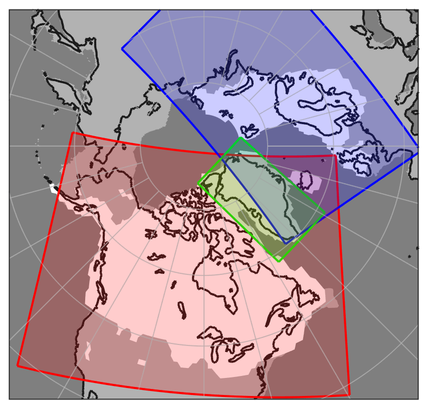
Figure 1 The extent of the North American (red), Greenland (green), and Eurasian (blue) domains. The present-day coastline is shown using black lines, while the land and ocean during the LGM are shown in grey. The extent of the LGM ice sheets described by Abe-Ouchi et al. (2015) is shown in white.

2.2 Climate forcing

To calculate the melting and accumulation of ice, our surface mass balance model (see Sect. 2.4) requires information on precipitation and temperature as functions of time and space. To efficiently compute climate forcing, we interpolate between pre-calculated pre-industrial (PI) and Last Glacial Maximum (LGM; 21 kyr ago) time slices using a matrix method (Pollard, 2010). This enables us to implicitly include climate–ice-sheet interactions at lower computational costs compared to fully coupled ice–climate set-ups. Details of this method, which is based on Berends et al. (2018) and Scherrenberg et al. (2023), are described in Appendix B.

The main drivers of temperature change are the external forcing and albedo, each contributing 50 % to the final temperature interpolation. External forcing is shown in Fig. 2a and is a combination of CO₂ (Fig. 2b; Bereiter et al., 2015) and insolation changes (Fig. 2c; Laskar et al., 2004). To derive an interpolation weight from this forcing, we first determine an index for CO₂, where 0 represents the LGM climate (190 ppm) and 1 represents the PI climate (280 ppm). We then modify this index using a 65° N summer insolation to capture changes in temperature caused by orbital cycles. Therefore, when summer insolation decreases, climate forcing approaches the LGM leading to cooling. The forcing index remains unchanged if the insolation is 440 W m⁻² (see Fig. 2a and c). As a result, for LGM CO₂ concentrations, the forcing index can still be relatively high for strong insolation, and for PI CO₂ levels, the forcing index can be relatively low for weak insolation values. We tuned the effect of insolation on the forcing index to capture the periodicity of glacial cycles over the past 800 000 years. To calculate the albedo feedback, we multiply the modelled surface albedo by the insolation to obtain the annual amount of insolation absorbed by the surface. We then calculate an interpolation weight from the concurrent amount of absorbed insolation and compare it to the fields obtained using LGM and PI climates and masks. The matrix method includes a precipitation–topography feedback as precipitation is interpolated with respect to local and domain-wide changes in the topography relative to the LGM and PI topography.

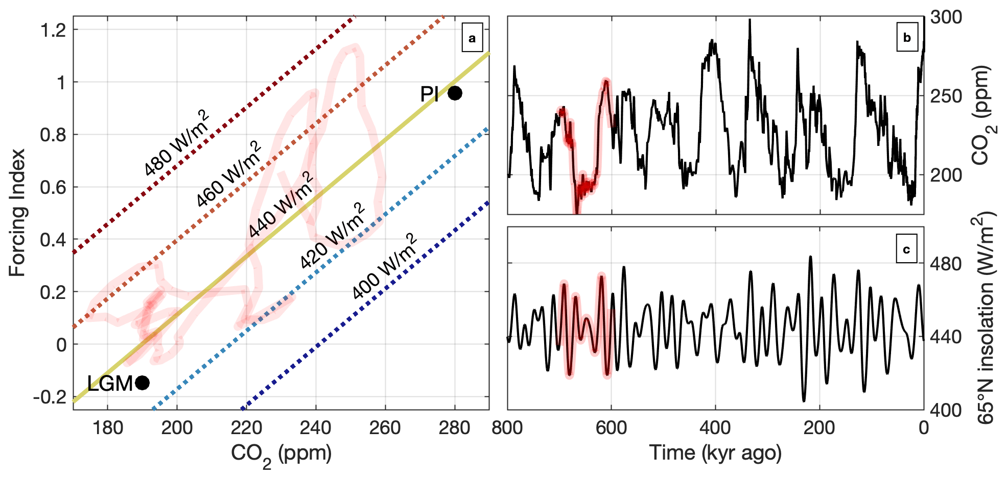
Figure 2 Panel (a) shows the forcing index, which combined with an albedo feedback, drives temperature changes in the ice-sheet model. The forcing index depends on the prescribed CO₂ (b; Bereiter et al., 2015) and insolation (c; Laskar et al., 2004). The pathway of the forcing index over a 100 kyr period is shown in red. A forcing index of 0 (1) represents the LGM (PI) temperature contribution from external forcing.

2.3 Climate time slices and downscaling

By simulating the last glacial cycle using an ice-sheet model, it has been shown that the LGM extent and volume were strongly dependent on climate forcing (Charbit et al., 2007; Niu et al., 2019; Alder and Hostetler, 2019; Scherrenberg et al., 2023). Not all general-circulation-model (GCM) simulations can be used to model an LGM ice-sheet extent that agrees well with reconstructions (Scherrenberg et al., 2023; Niu et al., 2019). Here, we use the mean of the MIROC (Sueyoshi et al., 2013), IPSL (Dufresne et al., 2013), COSMOS (Budich et al., 2010), and MPI (Jungclaus et al., 2012) members of phase 3 of the Paleoclimate Modelling Intercomparison Project (PMIP3; Braconnot et al., 2011). This ensemble has been shown to yield a good LGM extent in combination with IMAU-ICE (Scherrenberg et al., 2023). To correct biases in the GCM data, we calculate the difference between the PI time slice and the reanalysis from ERA-40 (Uppala et al., 2005). This bias is then applied to both the PI and LGM time slices. As a consequence, the resulting PI time slice may contain some of the anthropogenic warming present in ERA-40.

The topography and spatial resolution differ between the climate forcing and the ice-sheet model. Therefore, some corrections need to be applied before the climate forcing can be used in IMAU-ICE. First, we bilinearly interpolate the climate forcing onto the finer ice-sheet model grid. As the climate forcing has a lower resolution and therefore a smoother topography, some topographic corrections need to be applied to the temperature and precipitation fields. For temperature, we apply a lapse-rate-based correction. For precipitation, we use the Roe and Lindzen (2001) model to capture the orographic forcing of precipitation on the sloping ice margin and the plateau desert effect in the ice-sheet interior. A more detailed description of the bias correction and downscaling methods can be found in Appendix C.

2.4 Surface mass balance model

The surface mass balance (SMB) is calculated monthly using the insolation temperature model IMAU-ITM (Berends et al., 2018). For the present-day climate, this model provides an adequate SMB distribution, as shown in the Greenland Surface Mass Balance Model Intercomparison Project (GrSMBMIP; Fettweis et al., 2020). Using this model, the accumulation of snow is calculated using the large-scale snow–rain partitioning method proposed by Ohmura et al. (1999). Refreezing is calculated following schemes by Huybrechts and de Wolde (1999) and Janssens and Huybrechts (2000). Ablation is calculated based on Bintanja et al. (2002) and depends on temperature, insolation, and albedo. The equations describing this scheme (IMAU-ITM) are discussed in more detail in Appendix D.

3 Results

We conducted a “baseline” simulation by simulating North Hemisphere ice sheets from 782 ka to the present day. Figure 3a shows the extent of the ice sheets during the LGM compared to reconstructions of the North American ice sheet by Dalton et al. (2020) and the Eurasian ice sheet by Hughes et al. (2015; orange contours). The modelled LGM extent matches the reconstructions reasonably well, although ice coverage is lacking in the British Isles. A small proglacial lake formed in North America around 14 kyr ago (Fig. 3d). The North American ice sheet retreats faster than reconstructions suggest for the period starting 12 kyr ago (Fig. 3e–h), with full retreat occurring 10 kyr ago rather than 3 to 4 millennia later. Among other reasons (e.g.  uncertainty in the climate forcing, atmospheric circulation, and ice-sheet model parameterizations), this discrepancy could be partially due to the absence of feedback between meltwater, the ocean, and the climate. For example, prior to the Younger Dryas (12.9–11.7 kyr ago), large amounts of freshwater flowed into the North Atlantic (Teller et al., 2002; Tarasov and Peltier, 2005, 2006; Condron and Winsor, 2012), which could have caused a collapse in the Atlantic Meridional Overturning Circulation (AMOC), resulting in cooling (McManus et al., 2004; Velay-Vitow et al., 2024) and a stagnation in sea-level rise (Lambeck et al., 2014). At the present day (see Fig. 3i), the North American and Eurasian ice sheets have fully melted, with the exception of some small ice caps in regions that are currently partly glaciated (e.g. the Arctic Archipelago, Svalbard, and Iceland).

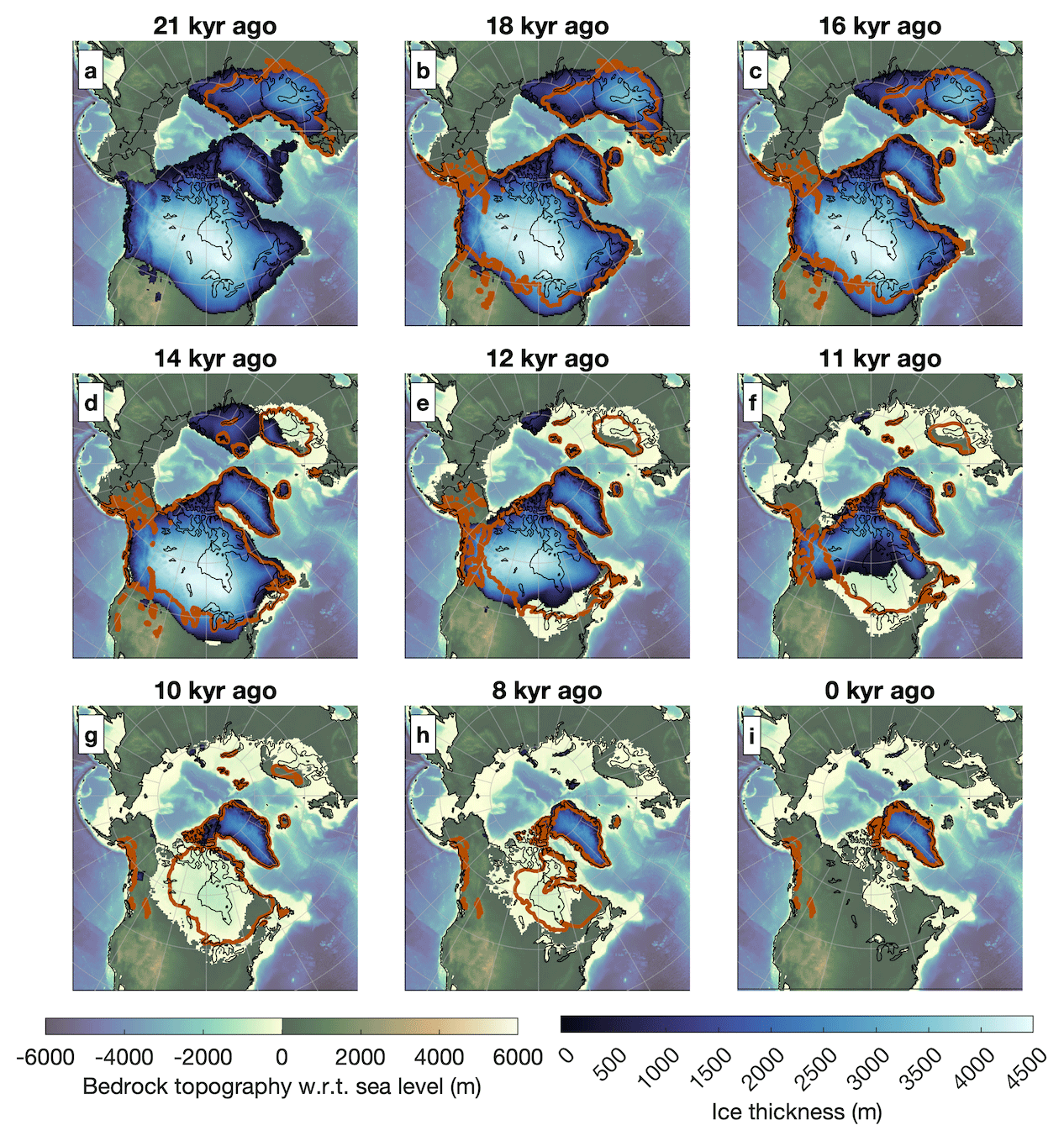
Figure 3 Ice thickness and bedrock topography from the baseline simulation during the last deglaciation. Reconstructions of the North American ice sheet by Dalton et al. (2020) and reconstructions of the Eurasian ice sheet by Hughes et al. (2015) are indicated by orange contours, while the present-day coastline is indicated by black contours. Please note that w.r.t stands for “with respect to”.

The total sea-level contribution of this baseline simulation is shown in Fig. 4, where it is compared to ice volume reconstructions by Spratt and Lisiecki (2016) and Grant et al. (2014). Since we only simulate Northern Hemisphere ice sheets, we added 30 % to the ice-sheet contribution to account for sea-level changes caused by phenomena other than the Northern Hemisphere ice sheets, such as the Antarctic (∼10 m), Greenland, and Patagonian ice sheets (Simms et al., 2019). While Antarctic ice volume has been shown to be correlated with Northern Hemisphere ice volume as sea-level changes prompt the advance and retreat of grounding lines (Gomez et al., 2020), this approach neglects out-of-phase behaviour of ice mass loss between the Northern and Southern hemispheres.

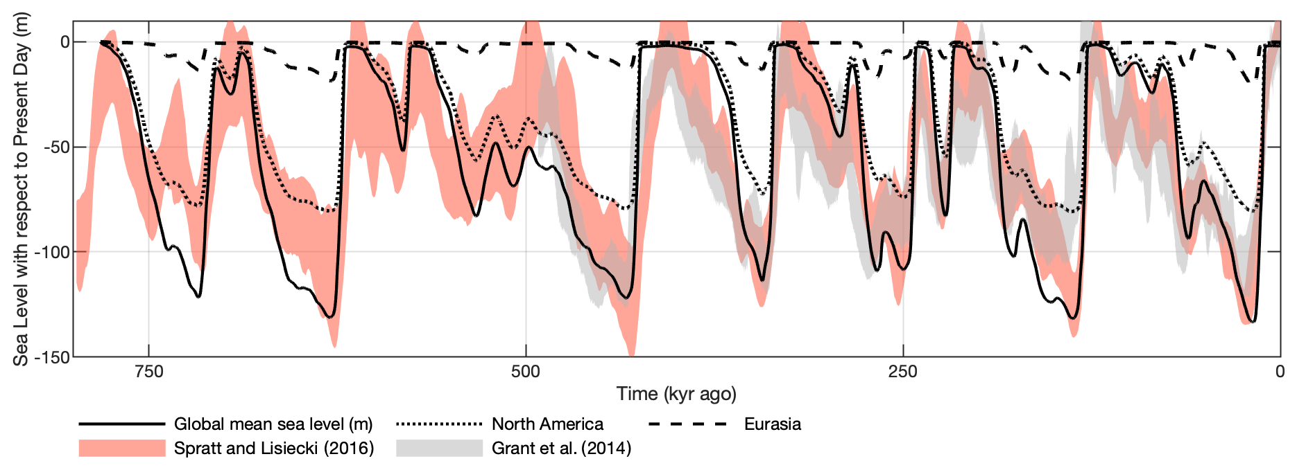
Figure 4 The simulated global mean sea level for the North American (dotted line) and Eurasian (dashed line) ice sheets, derived from the baseline experiment. The global mean sea-level change (solid line) represents the volume change from the Northern Hemisphere ice sheet plus an additional 30 % to account for other ice sheets (e.g. Patagonian, Himalayan, and Antarctic ice sheets). These results are compared with data from Grant et al. (2014) and Spratt and Lisiecki (2016).

We find that the modelled sea level captures all major melting events except Marine Isotope Stage (MIS) 13 (530–480 kyr ago), which had relatively low atmospheric CO₂ concentrations (∼240–250 ppm) compared to the interglacial periods that succeeded it (Siegenthaler et al., 2005; Bereiter et al., 2015). The modelled inception periods are longer compared to reconstructions, particularly for the warm interglacial MIS 11 (425–375 kyr ago). This results from the bias correction based on observations in which our PI time slice shows some anthropogenic warming. Consequently, modelled ice inception requires relatively low CO₂ concentrations and weak insolation. The ability of the model to capture the overall pattern of glacial terminations and fully melting North American and Eurasian ice sheets allows us to study the importance of ice dynamical processes that may have contributed to the decay of the ice sheets.

Figure 5 shows the ice volume time series for North America (Fig. 5b), Eurasia (Fig. 5c), and the Northern Hemisphere (Fig. 5a). Here, colours denote net melt (red) and net accumulation (blue), and black squares indicate the onset of deglaciation. In Fig. 5d–f, ice volume is plotted against climate forcing, with a glacial climate on the left and an interglacial climate on the right. As the climate becomes colder, the ice sheet tends to have a net positive mass balance and thus grows. However, as the ice sheet becomes larger and extends further towards the warmer south, CO₂ concentrations and insolation need to be lower to maintain net growth. This aligns with observations from Abe-Ouchi et al. (2013) and Parrenin and Paillard (2003), showing that a larger ice sheet is more vulnerable to increases in insolation and that deglaciation tends to take place when the ice volume is large enough.

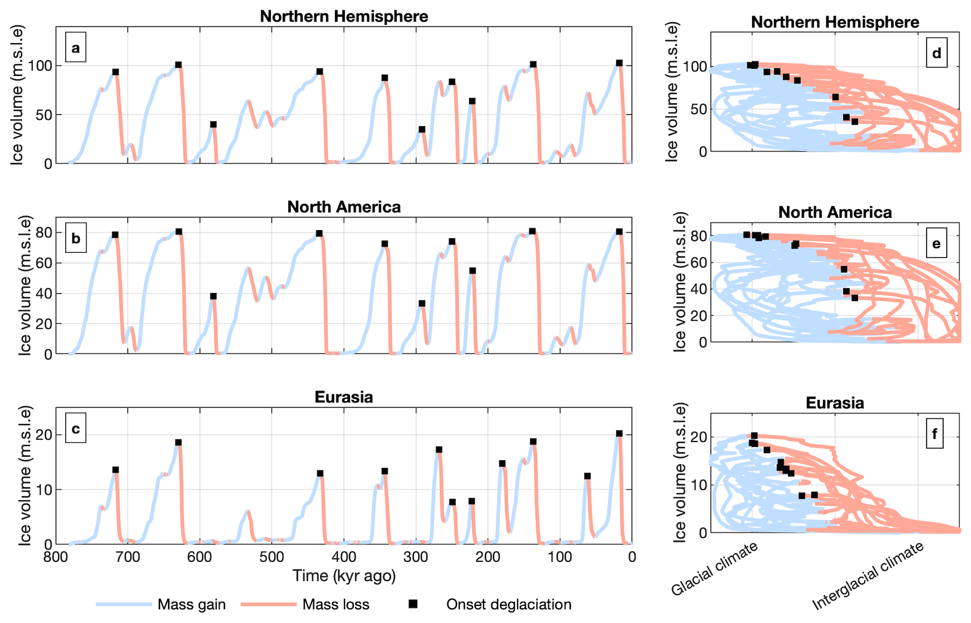
Figure 5 Time series of the simulated ice volume in the baseline experiment are shown in panels (a)–(c). Panels (d)–(f) show the ice volume along with the corresponding (glacial to interglacial) climate forcing, based on the external forcing (prescribed CO₂ and insolation forcing). Panels (a) and (c) show the combined ice volume of Eurasia, Greenland, and North America. Colours indicate net melt (red), net accumulation (blue), and the onset of deglaciation (black squares). The onset of deglaciation is only marked if the volume is at least 30 % of the simulation's maximum at the onset and falls below 30 % by the end of the termination.

The Eurasian ice sheet is more sensitive to collapse compared to the North American ice sheet. Occasionally, the Eurasian ice sheet melts completely (e.g. 168 kyr ago and 50 kyr ago), while the North American ice sheet only undergoes partial melting. This suggest that the Eurasian ice sheet is more vulnerable to complete melting during climate optima and that CO₂ concentrations and insolation can facilitate the decay of the Eurasian ice sheet while remaining favourable enough to allow the North American ice sheet to survive the climatic optimum. On average, the Eurasia ice sheet achieves full deglaciation roughly 3 millennia earlier than the North American ice sheet.

This is in line with the findings of Bonelli et al. (2009), Abe-Ouchi et al. (2013), and Tarasov and Peltier (1997), who found that the Eurasian ice sheet requires lower CO₂ concentrations or insolation levels compared to the North American ice sheet to survive climatic optima. The higher sensitivity of the Eurasian ice sheet is also supported by ice reconstructions, such as those by Gowan et al. (2021) and Mangerud et al. (2023), which show that the Eurasian ice sheet lost most of its volume during the MIS 3 interstadial period (60–25 kyr ago), while the North American ice sheet continued to survive until the LGM. This higher sensitivity of the Eurasian ice sheet to melting during a climate optimum may partly be due to its smaller size (the Eurasian sea-level contribution during the LGM is 19.1 m, compared to 80.1 m for the North American sea-level contribution) and higher LGM temperatures in the climate forcing, resulting largely from the thinner Eurasian ice sheet.

3.1 Design of the perturbed experiments

To investigate the effect of proglacial lakes and GIA on Late Pleistocene terminations, we carry out a set of experiments that are similar to the baseline experiment but with one process changed at a time. In the baseline set-up, our model reproduces the basic features of glacial terminations throughout the Late Pleistocene. For the sensitivity experiments, we modify the baseline simulation to investigate the effects of subshelf melting, basal friction of grounded ice, subshelf basal friction, and GIAs on the deglaciation of the Northern Hemisphere ice sheets. Each simulation starts at a point in time corresponding to 782 kyr ago, during an interglacial period when the North American and Eurasian continents were mostly ice-free. In the next few sections, we introduce these perturbation experiments to investigate which processes are important for the decay of the ice sheets. These experiments are described in Sect. 3.2–3.6 and summarized in Table 1.

Table 1 Descriptions of the experiments. Each perturbed experiment is similar to the baseline experiment, except for the described features.

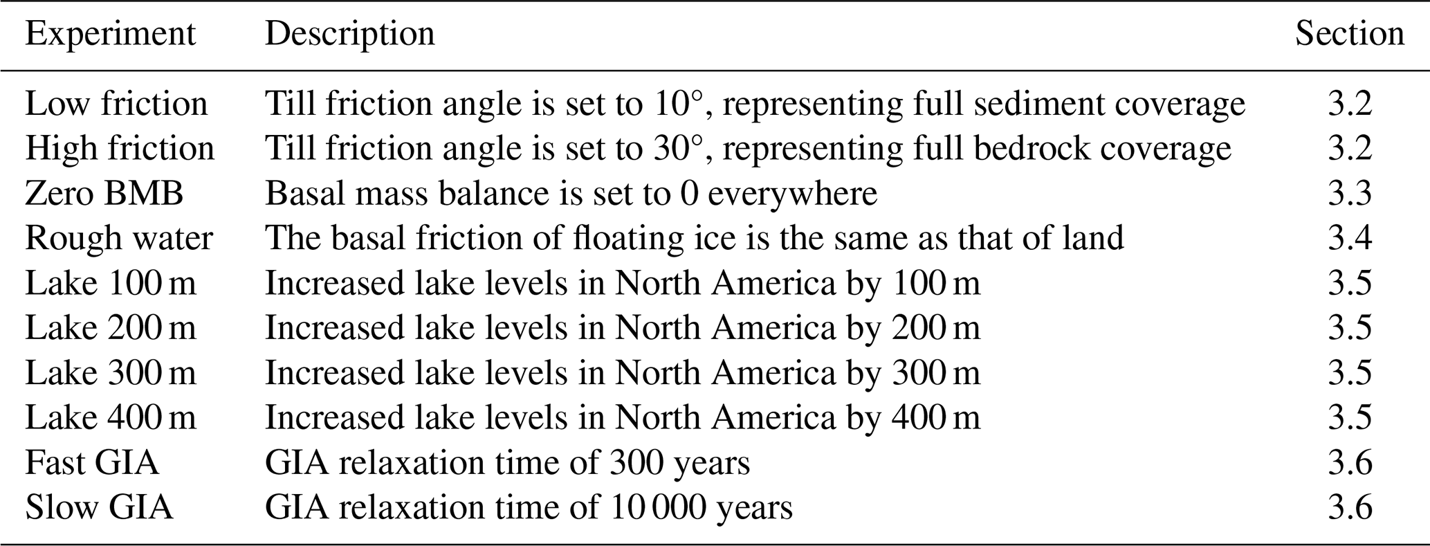
3.2 The effect of basal friction of grounded ice

The till friction angle is prescribed from and based on a geological map (Gowan et al., 2019; North America) and a sediment map (Laske and Masters, 1997; Eurasia). To assess the impact of basal friction on deglaciation, we conducted two sensitivity experiments. The first involves a low-friction simulation, with till friction angles set to 10° across the North American and Eurasian domains, and is a rough representation of continents fully covered by easily deformable sediments. The second involves a high-friction simulation that roughly represents full bedrock coverage, with till friction angles set to 30°. The basal hydrology is applied uniformly across all till friction angle maps and does not distinguish between sediment and bedrock.

Figure 6 shows a time series of the global mean sea-level contribution for the low-friction, baseline, and high-friction experiments. Figure 6b–k zoom in on individual glacial terminations. Basal friction has a substantial impact on deglaciation. As shown in Fig. 6, decreasing the till friction angle always results in an earlier completion of deglaciation. In the low-friction simulation, the peak melt rate in North America is achieved, on average, 4 centuries earlier compared to the baseline experiment, while in the high-friction simulation, the peak mass loss rate is achieved a millennium later (see Figs. S1 and S2 in the Supplement). In the low-friction scenario, the ice sheet fully melts at MIS 13, while in the high-friction scenario, full deglaciation is not achieved during MIS 13 or MIS 17 (712–676 kyr ago).

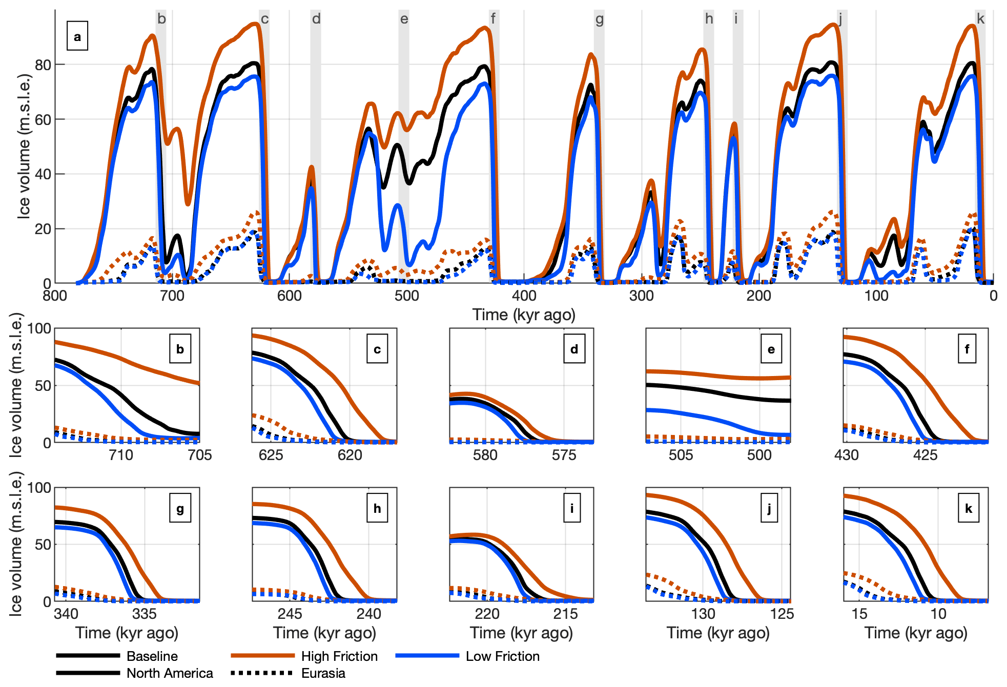
Figure 6 Ice volume time series (metres of sea level equivalent (s.l.e)) for the baseline, high-friction, and low-friction scenarios are shown in panel (a). Grey regions in panel (a) indicate the regions of the zoomed-in time series shown in panels (b)–(k).

Increasing friction also leads to increased ice volume at glacial maxima, although ice extent is not impacted as much. During the LGM, the North American global mean sea-level contribution in the high-friction simulation is 93.6 m, 17 % larger than the baseline simulation (80.1 m), while the low-friction simulation has a contribution of 75.3 m (6 % smaller). Similarly, the Eurasian sea-level contribution during the LGM is 19.1 m in the baseline simulation, 18.8 m in the low-friction simulation, and 23.7 m in the high-friction simulation. Figure 7 shows maps illustrating ice thickness in the baseline, low-friction, and high-friction simulations. Ice area during the LGM (Fig. 7a, f, and k) deviates by less than 1 % for North America and 3 % for Eurasia between simulations. Additional ice volume therefore mostly results from an increase in thickness (see Fig. 7a, f, and k). A time series comparing ice volume and area throughout the Late Pleistocene is shown in Fig. S3.

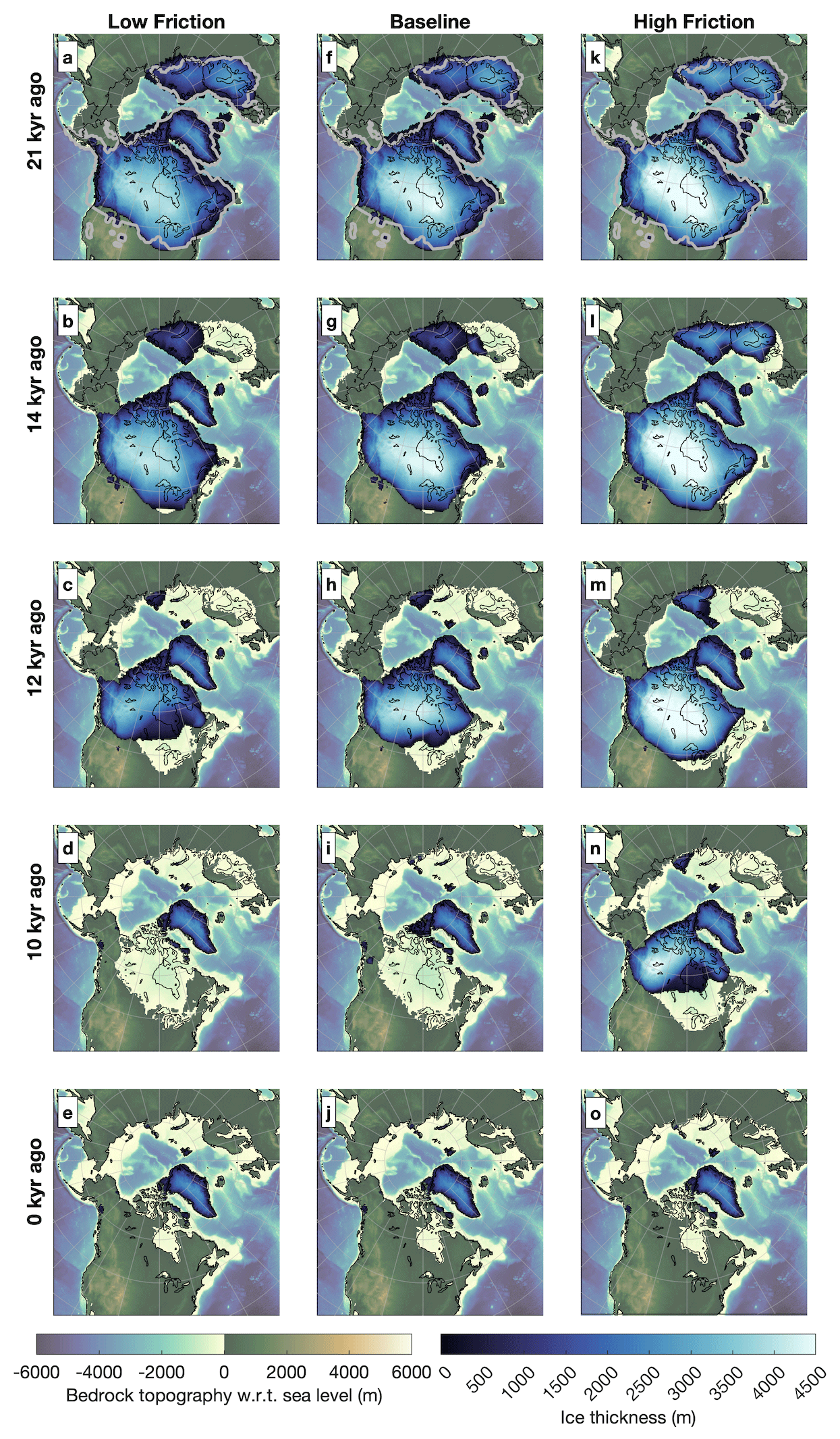
Figure 7 Ice thickness and bedrock topography for the low-friction (a–e), baseline (f–i), and high-friction (k–o) experiments. Time slices corresponding to 21 000 years (21 kyr) ago (a, f, k), 12 kyr ago (c–m), and 10 kyr ago (d–n) are shown. The LGM extent (a, f, k) from Abe-Ouchi et al. (2015) is indicated by grey contours, whereas black contours indicate the present-day coastlines.

These results suggest that basal friction has a large influence on melt rates during climate optima. Lower friction results in thinner ice sheets with gentler slopes, a large ablation area, and a lower SMB. Combined with increased ice velocities transporting more ice towards the ablation area, these processes can explain the increased sensitivity of the ice sheets during deglaciation and interstadial periods. As friction decreases, the ice sheets may become more sensitive to collapse during climate optima, which forms the basis of the regolith hypothesis, which suggests that the MPT may be explained by an increase in basal drag due to sediment being gradually removed during glacial cycles.

To study the robustness of our results, we also conducted the low-friction and high-friction experiments with the set-up used for the rough-water and fast-GIA simulations, discussed in Sect. 3.4 and 3.6 (see Figs. S4 and S5).

3.3 The effect of basal melting on glacial cycles

Proglacial lakes facilitate the formation of ice shelves, which can undergo subshelf melting. Subshelf melting is considered an important process in the current mass loss of Antarctica (Pritchard et al., 2012; Shepherd et al., 2018), where it is dominated by temperature and salinity gradients. Lake Agassiz, a freshwater lake created by the melting ice sheet, could therefore have substantially reduced basal-melt rates compared to parameterizations made for ocean shelves. Here, we conduct a sensitivity test to investigate whether subshelf melting has a significant impact on the retreat of the North American and Eurasian ice sheets.

The zero BMB experiment deviates from the baseline experiment as the subshelf-melt rate in North America and Eurasia is set to 0. Figure 8 shows the ice volume time series calculated in the zero BMB experiment and compares it to the baseline experiment. Figure 8b–k show the terminations in more detail. The zero BMB experiment is similar to the baseline experiment, although the ice sheets during glacial periods are slightly bigger and shelves can extend far into the ocean. During most terminations, removing subshelf melting only has a small effect, delaying full deglaciation by up to a millennium. MIS 13 and MIS 17 are exceptions. In MIS 17, substantially less ice is melted in the zero BMB experiment compared to the baseline experiment, with the lowest Northern Hemisphere sea-level contribution reaching 15.9 m in the zero BMB experiment and 4.0 m in the baseline experiment. Conversely, more ice is lost during MIS 13 in the zero BMB simulation, despite the lack of subshelf melting. This is caused by the increased sensitivity of the ice sheets when the ice volume is higher, as shown in the relationship between ice-sheet decay and climate forcing in Fig. 5. The zero BMB experiment has a substantially larger ice volume during the glacial period preceding MIS 13, and the retreat produces a substantial proglacial lake, which does not happen in the baseline experiment (see Fig. S6).

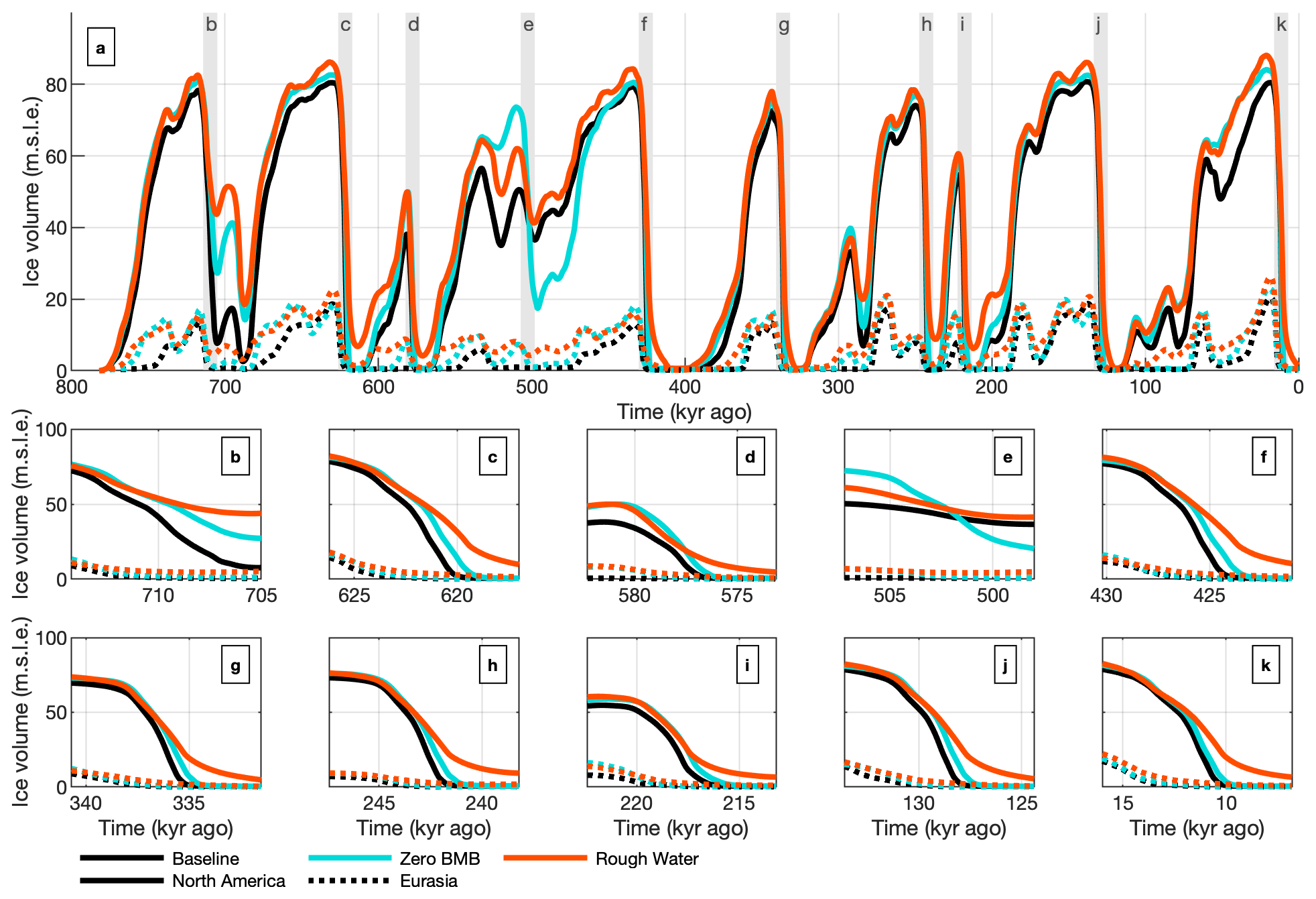
Figure 8 Time series of the North American and Eurasian ice sheets during various deglacial periods. The full 800 kyr time series is shown in panel (a). The grey regions in panel (a) correspond to the time series shown in panels (b)–(k).

3.4 The effect of basal friction on floating ice

The ice shelves floating on proglacial lakes or seas experience negligible basal friction, resulting in relatively high flow velocities. To study the impact of this lack of friction, we conduct the rough-water experiment. In this experiment, the subgrid friction coefficient is not scaled with the grounded fraction but is instead calculated as if all grid cells were grounded. Therefore, friction beneath shelves is not negligible anymore. This essentially prevents the formation of shelves, meaning that a migration of the grounding line does not cause a change in friction, which prevents PLISI/MISI. While this is a very unrealistic scenario, the grounding line does not migrate far into the ocean to cover the entire ice domain due to strong ablation, as shown in the ice thickness and bedrock topography maps in Fig. 9i–l.

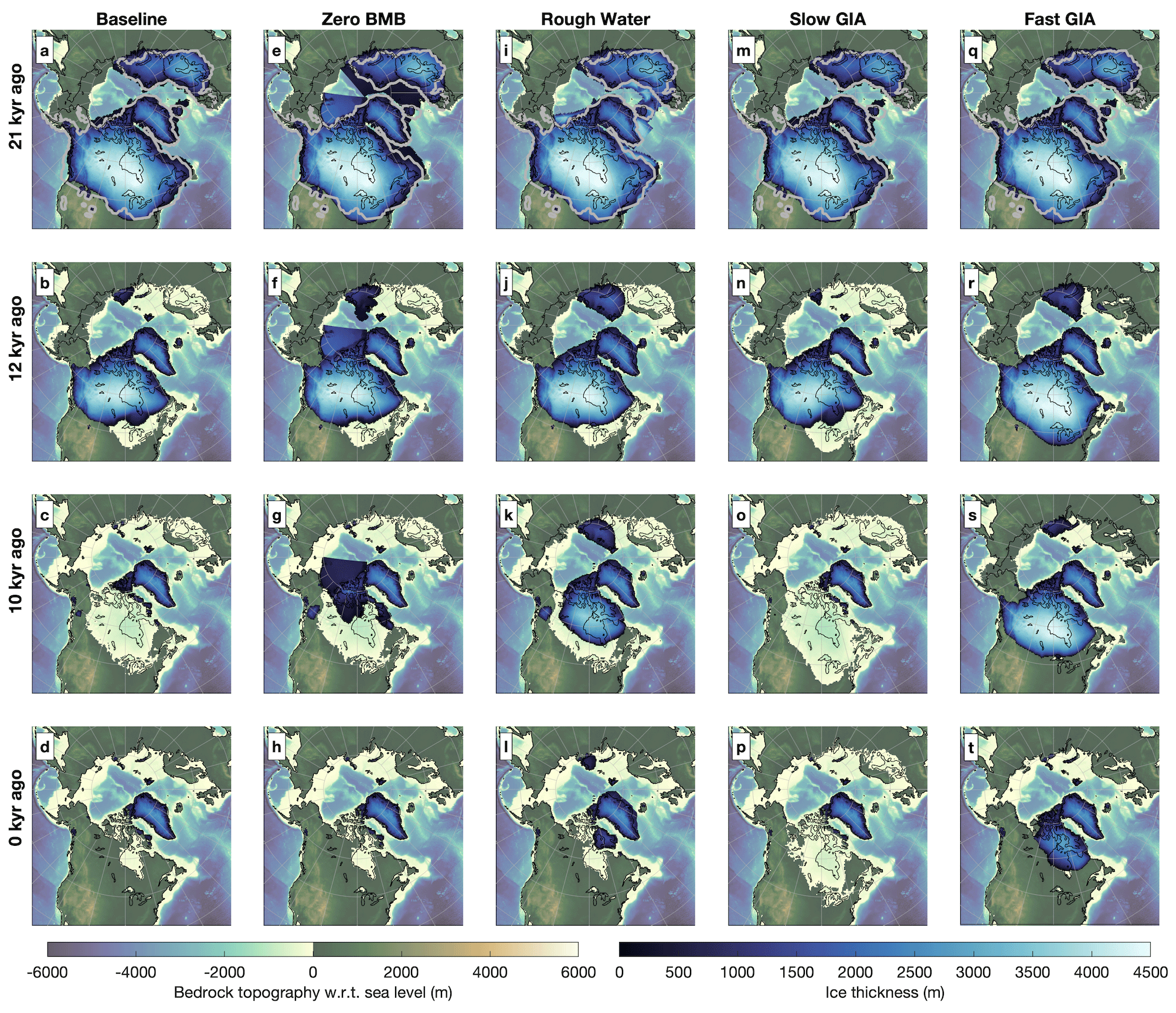
Figure 9 Bedrock topography and ice thickness in the baseline, rough-water, slow-GIA, and fast-GIA simulations (columns) corresponding to 21, 11, 9, and 0 ka (rows). The reconstruction from Abe-Ouchi et al. (2015) is shown in grey (a, e, i, m, q), and the present-day coastlines are shown in black.

The sea-level contribution in the rough-water experiment, shown in Fig. 8, can be compared to that in the zero BMB and baseline experiments. During the onset of the termination, the rough-water experiment loses mass at roughly the same pace as the baseline experiment. However, once more than half of the ice volume is lost, the mass loss rate in the rough-water experiment slows down with respect to the baseline experiment. This is because proglacial lakes are only created once the ice sheet has already partly retreated. Therefore, while the baseline and rough-water experiments have a similar retreat rate at the onset of the termination, the retreat in the baseline simulation accelerates once the proglacial lake has formed. Further differences between the rough-water and baseline simulations can be seen in the transect shown in Fig. 10. While the baseline simulation includes large ice shelves in North America, almost the entire ice sheet is grounded in the rough-water simulation. The shelves in the baseline simulation exhibit large ice velocities due to negligible subshelf friction. Consequently, the surfaces of the ice shelves in the baseline simulation are flat and close to sea level and therefore experience high temperatures and a strongly negative SMB. In the rough-water simulation, these shelves are very small. Without extensive shelves, higher elevation and steeper slopes result in a smaller ablation area.

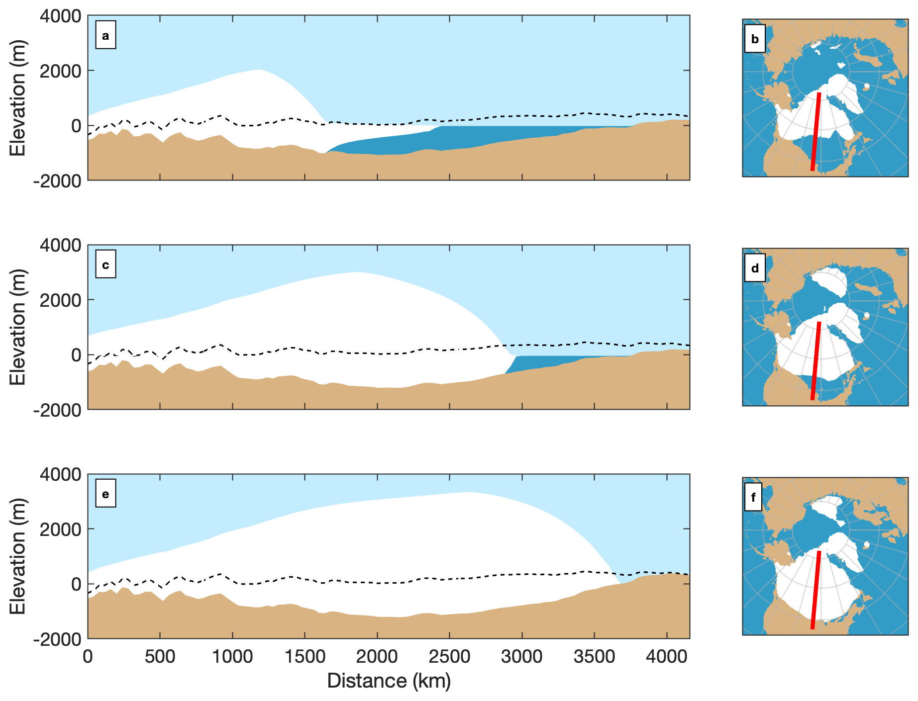
Figure 10 Transects (a, c, e) from the baseline (a, b), rough-water (c, d), and fast-GIA simulations (e, f) corresponding to 11 kyr ago. Present-day bedrock is indicated by dashed lines in panels (a), (c), and (e). The 0 km distance represents the northernmost point of the transect, as shown in panels (b), (d), and (f).

Interglacial ice volume is generally larger in the rough-water simulation compared to the baseline simulation. The Eurasian ice sheet only melts completely during glacial terminations and not during interstadial periods. Additionally, more ice tends to survive interglacial periods in both North America and Eurasia, which can be observed in the Barents–Kara Sea region and the Arctic Archipelago (see Fig. 9l). However, these results are sensitive to basal friction, and an increase in friction can lead to more ice surviving interstadial periods. In the high-friction equivalent of the rough-water experiment, neither the Eurasian nor the North American ice sheet fully deglaciate, with the smallest sea-level contributions corresponding to 4.5 and 11 m respectively (see Fig. S5).

3.5 Lake depth

Lakes are assumed to exist in the model wherever (glacial-isostatic-adjusted) bedrock is below the modelled sea level and where the modelled ice is thin enough to float. In the baseline experiment, the water level of the modelled lakes is assumed to be equal to sea level, while in reality, it can be significantly higher. To assess the effect of this simplifying assumption on our results, we simulate the last deglaciation (21 kyr ago to the present day) using a set of four different constant sea levels (relative to present-day levels) applied across the entire ice-sheet model grid (lake 100 m, lake 200 m, lake 300 m, and lake 400 m experiments). Therefore, lakes are simulated when bedrock is below these fixed sea levels, resulting in increased lake levels. As these sea levels are applied to the entire ice-sheet model grid, the experiments shown here overestimate the melt rates compared to a high-resolution lake model which allows for more drainage. Obviously, very high sea levels (e.g. 400 m) create an unrealistic inland sea that can hinder glacial inception. Therefore, we only apply these fixed levels for the last deglaciation and focus exclusively on the North American ice sheet. Despite this, even our most extreme scenario (400 m) does not induce an immediate collapse after the start of the simulation.

Time series of ice volume for the four lake-level experiments and the baseline experiment are shown in Fig. 11a. The evolution of the ice extent is shown in Fig. 11b–f, with colours indicating when each region of North America was last covered by ice. Here, we find that the retreat of the North American ice sheet occurs much faster with increasing sea levels, translating to a lead of roughly 1 millennium in terms of ice volume. These results indicate that lake levels significantly affect the rate of deglaciation for the North American ice sheet and that higher lake levels can substantially accelerate deglaciation.

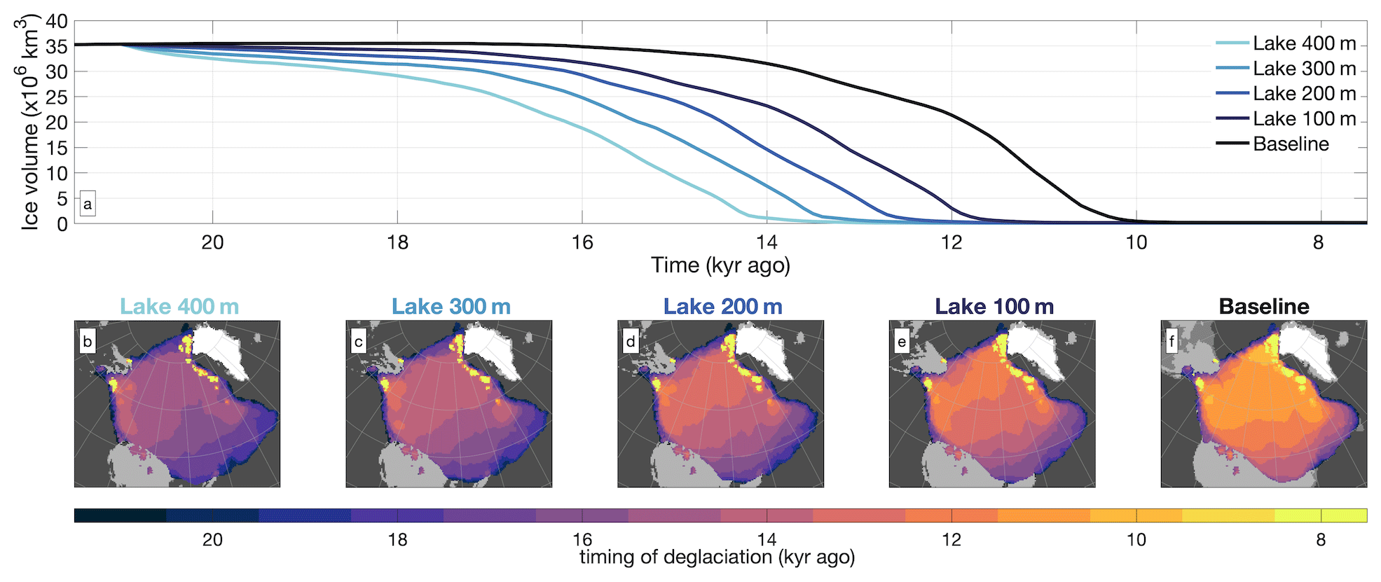
Figure 11 (a) Ice volume time series illustrating varying lake levels compared to the baseline simulation. Panels (b)–(f) show the timing of deglaciation. Background colours are coded from dark to light as follows: ocean in the LGM and PI time slices (dark grey), land in the LGM time slice but not in the PI time slice (grey), land in both the LGM and PI time slices (light grey), and present-day ice coverage (white).

3.6 Glacial isostatic adjustment

Proglacial lakes form through the interaction between GIA, ice sheets, and meltwater. Consequently, the GIA relaxation time controls how quickly bedrock fully recovers from changes in ice load. This relaxation time, as well as the thickness of the ice sheet and the retreat rate, controls the size and shape of the proglacial lake. Here, we assess the effect of GIA response time on multiple glacial cycles while modelling PLISI. We compare three simulations: the previously shown baseline simulation (3000 years), the slow-GIA simulation (10 000 years), and the fast-GIA simulation (300-year relaxation time).

Figure 12 shows the ice volume time series for these three simulations, with smaller panels zooming in on individual terminations (Fig. 12b–k). The retreat in the slow-GIA simulation is generally slower and can lag up to a millennium behind the baseline simulation in terms of ice volume. However, some deglaciations (e.g. the last and penultimate deglaciations) exhibit minimal differences compared to the baseline simulation. This can be explained by differences in the bedrock topography at the onset of the deglaciations and the presence of proglacial lakes. The slower subsidence rates in the slow-GIA simulations may result in higher bedrock topographies. This reduces the modelled saturation at the base as saturation increases with a decreasing bedrock topography relative to the concurrent sea level. Therefore, in the slow-GIA simulation, basal friction may be lower at the onset of some terminations, causing reduced retreat rates. However, if the bedrock topography during a glacial maximum is similar to that in the baseline simulation, the retreat will also be similar (see Fig. 12c, j, and k). An exception is MIS 13, where the North American ice sheet fully melts in the slow-GIA simulation but not in the baseline simulation. Retreat rates and ice-sheet volume are not sufficient to induce a proglacial lake in the baseline simulation. However, in the slow-GIA simulation, slower bedrock uplift allows for the creation and sustainment of a proglacial lake throughout this termination event, enabling the North American ice sheet to fully melt (see Fig. S6).

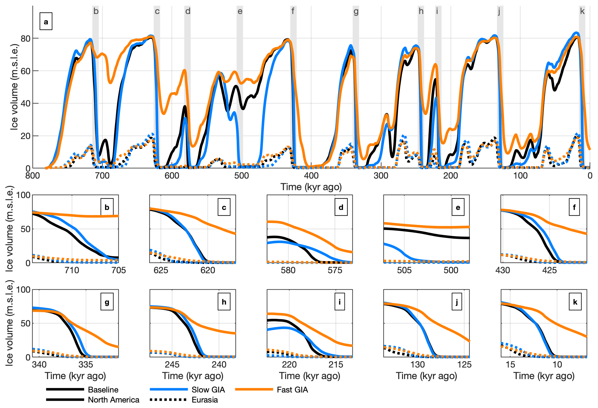
Figure 12 Time series illustrating ice volume with different GIA relaxation times. The time series for the past 800 kyr is shown in panel (a). Panels (b)–(k) each show one termination, indicated by the grey regions in panel (a).

The ice thickness and bedrock topography in the slow-GIA simulations corresponding to 21, 12, 10, and 0 kyr ago are shown in Fig. 9m–p. During the retreat, the proglacial lakes are significantly larger compared to those in the baseline simulation as bedrock uplift is slower. The slow-GIA simulation also has a delayed onset phase, as seen in Fig. 12. Due to the slow bedrock uplift, large parts of North America still remain below sea level millennia after the ice sheet fully receded (see Fig. 9p). As a result, regions such as northeastern Canada, a key location for ice inception, remained below sea level throughout the entire preceding interglacial period.

The fast-GIA simulation exhibits substantially slower melt rates compared to the baseline, slow-GIA, and rough-water simulations, as shown in the transects in Fig. 10 and the ice thickness maps in Fig. 9q–t. The delayed deglaciation is due to two processes. Firstly, as the ice sheet retreats, rapid bedrock rebound quickly eliminates the depression left by the ice sheet, preventing the formation of proglacial lakes (see Fig. 9q–t). Secondly, the reduction in ice thickness is more efficiently compensated for by the bedrock rebound, which reduces the elevation–temperature feedback, thereby reducing surface melt rates and slowing deglaciation. Therefore, while the fast-GIA and rough-water simulations eliminate the effects of proglacial lakes, only the fast-GIA simulation reduces melt rates from the onset of the termination. During many interglacial periods, including the present, an ice dome persists or the termination is skipped. However, this is again strongly dependent on basal friction: the low-friction equivalent of the fast-GIA experiment induces full melting during most interglacial periods, while the high-friction equivalent never melts completely (see Figs. S4 and S5). The lack of lakes, combined with the SMB–elevation feedback, makes the fast-GIA simulation the one with the slowest deglaciation.

4 Discussion

In this study, we investigate the effect of proglacial lakes on the deglaciation of the Eurasian and North American ice sheets throughout the past 800 kyr. In the baseline configuration, the modelled ice volume over time generally agrees well with different sea-level reconstructions, meaning that all major deglaciations throughout the Late Pleistocene are captured. However, shortcomings include the lack of ice coverage over the British Isles and the fact that our simulations tend to produce interglacial periods that are too long compared to reconstructions. This is especially evident for the MIS 11 interglacial period, which exhibits higher global temperatures and sea levels compared to the present day (Hearty et al., 1999; Raymo and Mitrovica, 2012). Warmer-than-pre-industrial temperatures are also not captured as our climate forcing was interpolated from PI and LGM time slices. Adding additional time slices to our matrix method, similar to the approach used by Abe-Ouchi et al. (2013), especially for warmer conditions than those of the present day, may improve our representation of various ice volume, CO₂ concentration, and orbital parameters. Results nevertheless depend strongly on the quality of the climate forcing (Scherrenberg et al., 2023). Here, we chose a forcing that results in an LGM extent that agrees well with reconstructions, rather than including a large number of time slices.

The size and shape of proglacial lakes result from the interaction between GIA and ice thickness. Here, we used uniform GIA response times, but in reality, GIA varies spatially (e.g. Forte et al., 2010; van Calcar et al., 2023) and has large uncertainties. GIA can increase the size of proglacial lakes compared to scenarios without GIA (e.g. Austermann et al., 2022), and in this study, we demonstrated that increasing the GIA response time leads to proglacial lakes being larger. A faster GIA response decreases the size of proglacial lakes, and increased bedrock uplift can partly compensate for thickness loss, resulting in reduced melt rates.

Here, we simulated lakes where bedrock is situated below sea level. This is a simplification as lakes can exist well above sea level, and, as shown in the lake 100–400 m experiments, increasing lake levels results in substantially faster deglaciation. Lake models and drainage algorithms incur high computational costs when applied at a fine topographic resolution that captures all valleys and drainage channels. While this may not be feasible, computational costs could be reduced by asynchronously coupling with a flood-fill algorithm (Berends and van de Wal, 2016) or using a drainage algorithm (Tarasov and Peltier, 2006) at a reduced spatial resolution. These methods do not capture every drainage channel; however, they may give a reasonable estimate of lake levels and thus may improve the current method.

In this study, we treated lakes as if they were oceans. However, as lakes have lower salinity levels and are smaller in size, they can exhibit substantially different types of subshelf melting (Sugiyama et al., 2016) and lower calving rates (e.g. Warren et al., 1995; Warren and Kirkbride, 2003; Benn et al., 2007), and the clogging of icebergs can create a potential buttressing effect (Geirsdóttir et al., 2008). These limitations suggest that the effects of basal melting and calving may be overestimated in the proglacial lakes, and they are further compounded by uncertainties in the subshelf-melting and calving schemes used here. For example, applying a more sophisticated subshelf-melting scheme which simulates high melt rates near the grounding line (Rignot and Jacobs, 2002) may result in a greater impact from subshelf melting. Additionally, we have not explored the effect of calving rates in detail; however, as shown by Cutler et al. (2001), lake calving can have an effect on the ice flow of the Laurentide ice sheet. Nevertheless, our results suggest that while subshelf melting can enhance the melting of the North American and Eurasian ice sheets, it is overshadowed by large surface melt rates and PLISI. Due to these limitations, we cannot give an exact estimate of how much longer a deglaciation phase will take when subshelf melting is removed; however, our findings serve as an indication that full melting can still take place without subshelf melting.

Another limitation is the treatment of basal friction. For basal hydrology, we used a parameterization from Martin et al. (2011), and the till friction angle was based on geology and sediment masks. We performed experiments by decreasing the till friction angle to 10 or 30°, representing full sediment or full hard-bed coverage. We found that these changes significantly influence ice volume at glacial maxima, with a much smaller effect on ice extent. Deglaciation is also slower with increasing friction. While our main conclusions are consistent across various basal-friction scenarios, the timing of deglaciation and the ice volume that persists through interglacial periods differ substantially. This highlights that the volume of the glacial cycle and melt rates are sensitive to basal friction. Here, we used a static till friction angle mask. However, friction can change over time as bedrock is eroded and sediment is transported. Basal friction could therefore be improved by including a sediment transport model (e.g. Hildes et al., 2004; Melanson et al., 2013) and a more sophisticated basal-hydrology method (e.g. Hoffman and Price, 2014; Flowers, 2015).

The matrix method used to interpolate between the LGM and PI time slices implicitly includes temperature–albedo and precipitation–topography feedbacks. However, ice-sheet–climate interactions can exhibit threshold behaviours which cannot be simulated using our method. These behaviours include the opening and closing of straits, such as the Canadian Arctic Archipelago (Löfverström et al., 2022); the response of Heinrich and Dansgaard–Oeschger events (Claussen et al., 2003); and rapid changes in ocean circulation and sea ice due to the influx of meltwater into the ocean (Otto-Bliesner and Brady, 2010). Since we do not model the ocean, there are no interactions between meltwater, ocean circulation, and the climate. This may partially explain why the baseline simulation shows excessively high retreat rates from 12 kyr ago, coinciding with the Younger Dryas. The Younger Dryas exhibits reduced rates of sea-level rise (e.g. Lambeck et al., 2014) and lower Northern Hemisphere temperatures due to a stagnation of the AMOC (McManus et al., 2004; Velay-Vitow et al., 2024), likely caused by an influx of meltwater into the North Atlantic (Teller et al., 2002; Tarasov and Peltier, 2005, 2006; Condron and Winsor, 2012). This process is not included in our set-up as temperature is only affected by CO₂, insolation, elevation and albedo; therefore, it fails to capture the stagnation in melt rates observed during the Younger Dryas.

Including many of these behaviours would require a model that more explicitly simulates the climate system. GCMs may be able to simulate these interactions, but simulating glacial cycles with a reasonably high resolution would require an excessive number of computational resources. Alternatively, ocean–atmosphere circulation models can be used to simulate individual glacial terminations (Obase et al., 2021), or intermediate-complexity models (Ganopolski and Calov, 2011) can simulate multiple glacial cycles with more explicit feedbacks in the climate system; however, these approaches still require higher computational costs than ice-sheet models and more parameterizations than full GCMs.

5 Conclusion

We studied the relative importance of different ice dynamical processes for glacial terminations. The onset of terminations is dominated by a decrease in the SMB, which causes the retreat of the ice sheet. We found that the Eurasian ice sheet requires lower CO₂ concentrations and/or insolation compared to the North American ice sheet in order to survive a climate optimum. Once the ice sheets have retreated significantly, proglacial lakes are created at the margin of the ice sheets. Our results show that these proglacial lakes can significantly accelerate the collapse of the North American and Eurasian ice sheets. If certain processes facilitated by the lakes are removed, the North American and Eurasian ice sheets deglaciate at a reduced pace and may remain partially covered in ice during interglacial periods.

The largest impact of proglacial lakes on deglaciation is their facilitation of low friction under floating ice. If the basal friction of shelves is the same as that of grounded ice, removing the effects of PLISI and MISI, the Eurasian ice sheet only fully melts during interglacial periods rather than during interstadial periods. Additionally, more ice may persist in the Northern Hemisphere during interglacial periods. The high ice velocities caused by negligible subshelf friction create large shelves with low surface elevations, leading to high temperatures and surface melt. However, this process is also sensitive to basal friction. Lowering basal friction decreases ice thickness at glacial maxima, and, consequently, surface temperatures and melting increase. Therefore, reduced friction results in faster deglaciation. This shows that modelling sediments and hydrology is important for simulating glacial cycles. Furthermore, we found that subshelf melting is only a secondary effect with respect to the mass loss of the ice sheets. Applying a zero subshelf-melt rate still results in full deglaciation, although it may take an additional millennium for it to be completed.

We also investigated the effect of the GIA response time on consecutive glacial cycles and deglaciations. If the GIA response is slower than in our baseline simulation, the termination can be slower by up to a millennium, and the subsequent inception phase is delayed. Since inception sites are typically the last regions to deglaciate, land may remain below sea level at the onset of the next glacial period if the bedrock rebound is too slow. We find that a GIA response that is substantially faster than the baseline simulation results in slower deglaciation and larger interglacial ice volumes as the North American and Eurasian ice sheets may not fully deglaciate during some interglacial periods. This is because proglacial lakes are not created when bedrock uplift is too fast. Additionally, surface melt is reduced as bedrock uplift compensates for ice thickness loss more efficiently.

When projecting the future mass loss of the Greenland and Antarctic ice sheets, marine-ice-sheet dynamics and ice-sheet–climate interactions are considered very important. For Antarctica, the marine equivalent of PLISI, MISI, may induce a runaway collapse of parts of the West Antarctic Ice Sheet (e.g. Ritz et al., 2015). However, this is not a perfect analogy as, for example, the high sensitivity of the Eurasian ice sheet to temperature does not directly translate to future melting in West Antarctica (van Aalderen et al., 2024). The Greenland ice sheet is currently mostly land-terminating, but proglacial lakes are created during the retreat – a phenomenon that is already being observed (e.g. Carrivick and Quincey, 2014). These lakes may accelerate the retreat of the Greenland ice sheet (Carrivick et al., 2022). Therefore, our results underline the relevance of these processes in understanding past ice-sheet evolution and highlight the importance of reproducing this evolution to help constrain these processes in the context of current changes in Antarctica and Greenland.

Appendix A: Basal sliding, friction, and hydrology

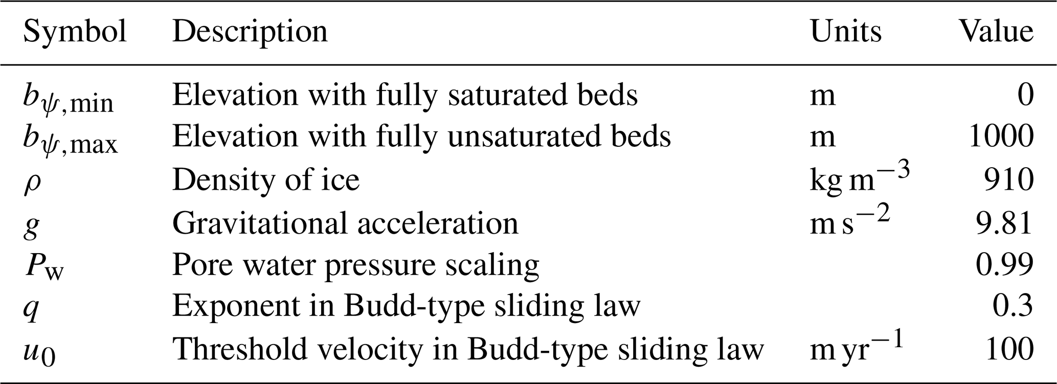
In this study, we used a Budd-type sliding law to simulate the sliding at the base of the ice sheets. To calculate the friction underneath the base of the ice sheet, we applied a parameterization based on Martin et al. (2011). Table A1 lists the units and corresponding values of the constants named here.

The pore water pressure (ψ) is parameterized based on Martin et al. (2011). The pore water pressure scaling factor (λ) determines the saturation of the base and depends on the local bedrock height (b) and the concurrent sea level (SL). It is expressed as

$$\begin{array}{}\text{(A1)}& \mathit{\lambda }=\mathrm{1}-{\displaystyle \frac{b(x,y)-\mathrm{SL}-b_{\mathit{\psi },\min }}{b_{\mathit{\psi },\max }-b_{\mathit{\psi },\min }}},\end{array}$$

where x and y represent the horizontal grid indices. The pore water pressure scaling factor is limited between 1 (fully saturated) and 0 (fully unsaturated). Here, b_ψ,max is the bedrock elevation at which the beds become fully unsaturated (1000 m), relative to sea level, while b_ψ,max is the elevation at which the beds become fully saturated (0 m). This pore water pressure scaling factor is used in combination with the overburden pressure to calculate the pore water pressure (ψ), which is given by

$$\begin{array}{}\text{(A2)}& \mathit{\psi }=P_{\mathrm{w}}\mathit{\rho }gH(x,y)\mathit{\lambda }.\end{array}$$

Here, H represents the thickness of the ice and P_w is the pore water pressure scaling fraction. Here, we use a value of 0.99, which yields a reasonable modelled LGM ice-sheet volume and extent in combination with the prescribed till friction map. To determine the till friction angle (ϕ), we use different data sets for North America and Eurasia. For North America, we use a geology reconstruction from Gowan et al. (2019), which provides full coverage of our ice domain and indicates where bedrock could be more easily eroded. The map from Gowan et al. (2019) has been specifically created for ice-sheet modelling. For Eurasia, we created a till friction angle map based on sediment thicknesses from Laske and Masters (1997). Here, till friction angles are 10° when sediment thicknesses exceed 100 m, while for other regions, till friction angles of 30° are used. In the high-friction simulations, till friction angles are 30° in North America and Eurasia, while the low-friction simulations have till friction angles of 10°. For Greenland, which is not the focus of our experiments, we always use a till friction angle map with values of 30° for present-day land and 10° for oceans. The pore water pressure and till friction angle can then be used to calculate the till yield stress (τ), expressed as

$$\begin{array}{}\text{(A3)}& \mathit{\tau }(x,y)=\tan \left({\displaystyle \frac{\mathit{\pi }}{\mathrm{180}}}\right)\mathit{\varphi }\left(\mathit{\rho }gH\right(x,y)-\mathit{\psi }).\end{array}$$

To calculate the basal-friction coefficient (β), we use the Budd-type sliding law (Bueler and van Pelt, 2015), which is given by

$$\begin{array}{}\text{(A4)}& \mathit{\beta }\left(xy\right)=\mathit{\tau }(x,y){\displaystyle \frac{u^{(q-\mathrm{1})}}{u_{\mathrm{0}}^q}}.\end{array}$$

Here, u represents the ice velocity. The sliding term, is then used to calculate the basal sliding. The basal-friction coefficient is multiplied by the grounded fraction, which is calculated based on Leguy et al. (2021). Therefore, regions that are fully floating (grounded fraction of 0) receive negligible friction, the grounding line (grounded fraction between 0 and 1) receives reduced friction, and fully grounded ice receives full friction (grounded fraction of 1). In the rough-water simulation, the basal-friction coefficient is always multiplied by 1, which means friction is applied as if all ice were grounded.

Table A1 Constants describing till friction angle and basal hydrology.

Appendix B: Climate time slice interpolation

To provide the ice-sheet model with transiently changing forcing using minimal computational resources, we interpolate between pre-calculated LGM and PI climate time slices. To interpolate the time slices, we use a matrix method. Our approach is based on Berends et al. (2018) and Scherrenberg et al. (2023) and uses different methods for temperature and precipitation.

To calculate the temperature forcing, we use linear interpolation:

$$\begin{array}{}\text{(B1)}& \begin{array}{rl}T(x,y,\mathrm{mnth})& =w_{\mathrm{T}}(x,y)T_{\mathrm{PI}}(x,y,\mathrm{mnth})\\ & +\left(\mathrm{1}-w_{\mathrm{T}}(x,y)\right)T_{\mathrm{LGM}}(x,y,\mathrm{mnth}).\end{array}\end{array}$$

Here, T is the monthly (mnth) temperature forcing in the ice-sheet model. T_PI and T_LGM are the climate model temperatures for the PI and LGM time slices respectively. Moreover, w_T is the interpolation weight and depends on two processes: external forcing (w_e) and albedo feedback (w_a). To prevent excessive extrapolation, w_T is capped between −0.25 and 1.25. For North America and Eurasia, w_T is calculated as follows (see Berends et al., 2018):

$$\begin{array}{}\text{(B2)}& w_{\mathrm{T}}(x,y)={\displaystyle \frac{w_{\mathrm{e}}(x,y)+w_{\mathrm{a}}(x,y)}{\mathrm{2}}}.\end{array}$$

In Greenland, albedo changes are almost exclusively due to changes in the ice-sheet extent. Our model does not include sea ice, and the Greenland domain does not contain extensive tundra areas. Therefore, we apply a smaller albedo contribution, expressed as

$$\begin{array}{}\text{(B3)}& w_{\mathrm{T}}(x,y)={\displaystyle \frac{\mathrm{3}{w}_{\mathrm{e}}(x,y)+w_{\mathrm{a}}(x,y)}{\mathrm{4}}}.\end{array}$$

To calculate w_e, we combine the effects of CO₂ concentration (ppm; Bereiter et al., 2015) and insolation at 65° N (Q_65° N; W m⁻²; Laskar et al., 2004):

$$\begin{array}{}\text{(B4)}& w_{\mathrm{e}}={\displaystyle \frac{C-C_{\mathrm{LGM}}}{C_{\mathrm{PI}}-C_{\mathrm{LGM}}}}+{\displaystyle \frac{Q_{\mathrm{65}\mathit{°}\mathrm{N}}-\mathrm{440}\mathrm{W}{\mathrm{m}}^{-\mathrm{2}}}{\mathrm{70}\mathrm{W}{\mathrm{m}}^{-\mathrm{2}}}}.\end{array}$$

In this equation, C_PI and C_LGM correspond to 190 and 280 ppm respectively. By including summer (June–July–August) insolation at 65° N (Q_65° N), the climate can become colder or warmer even if the CO₂ concentration is constant (see Fig. 2). We obtained the ratio between CO₂ and insolation by first conducting a preliminary simulation based on the methods from de Boer et al. (2013) and Berends et al. (2021a), where forcing was modified to match the benthic δ¹⁸O record from Ahn et al. (2017). This approach essentially reproduces the forcing needed to match the benthic δ¹⁸O record. We then fitted CO₂ and summer insolation to this forcing to obtain Eq. (B4).

To calculate w_a, which represents albedo feedback, we calculate the annual insolation absorbed by the surface. The absorbed insolation (I) depends on the monthly internally calculated surface albedo (α_s) and insolation at the top of the atmosphere (Q). I(x,y) is given by

$$\begin{array}{}\text{(B5)}& I(x,y)=\sum _{m=\mathrm{1}}^{\mathrm{12}}Q(x,y,\mathrm{mnth})\left(\mathrm{1}-{\mathit{\alpha }}_{\mathrm{s}}(x,y,\mathrm{mnth})\right).\end{array}$$

The albedo is calculated in the ice-sheet model using Eq. (D3). To calculate an interpolation weight for the absorbed insolation (w_i), we need to calculate reference fields for the LGM and PI time slices. To calculate the albedo for the LGM time slice, we use land and ice masks from the ice-sheet reconstruction by Abe-Ouchi et al. (2015) as these were also used in the climate model simulations. We integrate the SMB model forward through time with a fixed climate and ice-sheet geometry until the firn layer reaches a steady state (typically after ∼30 years). We can then use Eq. (B5) to calculate the reference fields for the absorbed insolation. These absorbed-insolation fields can then be used to calculate w_i.

$$\begin{array}{}\text{(B6)}& w_{\mathrm{i}}(x,y)=\left(I(x,y)-I_{\mathrm{LGM}}(x,y)\right)/\left(I_{\mathrm{PI}}\left(xy\right)-I_{\mathrm{LGM}}\left(xy\right)\right)\end{array}$$

To account for both local and domain-wide changes in albedo and insolation, we use the following equation based on Berends et al. (2018):

$$\begin{array}{}\text{(B7)}& w_{\mathrm{a}}(x,y)={\displaystyle \frac{w_{\mathrm{i}}(x,y)+\mathrm{3}{w}_{\mathrm{i},\mathrm{smooth}}(x,y)+\mathrm{3}{w}_{\mathrm{i},\mathrm{domain}}(x,y)}{\mathrm{7}}}.\end{array}$$

Here, w_i,domain is the domain-wide-averaged interpolation weight and w_i is the local interpolation weight. Moreover, w_i,smooth represents the regional temperature effect and is calculated by applying a 200 km Gaussian smoothing filter to w_i. Once again, we use a different method for Greenland due to the lack of tundra regions; this method is expressed as

$$\begin{array}{}\text{(B8)}& w_{\mathrm{a}}(x,y)={\displaystyle \frac{w_{\mathrm{i},\mathrm{smooth}}(x,y)+\mathrm{6}{w}_{\mathrm{i},\mathrm{domain}}}{\mathrm{7}}}.\end{array}$$

The interpolation weight used to calculate temperature (w_T) can now be derived from w_a and w_e using Eqs. (B2) or (B3). This interpolation weight changes depending on albedo, insolation, and CO₂.

For precipitation, we apply a different method as precipitation does not change linearly when the climate cools down and the topography changes. We use the following equation to interpolate precipitation from the climate time slices:

$$\begin{array}{}\text{(B9)}& \begin{array}{rl}P& =\exp \left(\left(\mathrm{1}-w_{\mathrm{P}}(x,y)\right)\log \left(P_{\mathrm{PI}}(x,y,\mathrm{mnth})\right)\right.\\ & \left.+w_{\mathrm{P}}(x,y)\log \left(P_{\mathrm{LGM}}(x,y,\mathrm{mnth})\right)\right).\end{array}\end{array}$$

Here, w_P is the interpolation weight and depends on local and domain-wide topography changes. First, we compare the domain-wide topography in the model to the climate time slices using the following equation:

$$\begin{array}{}\text{(B10)}& \begin{array}{rl}{w}_{\mathrm{s},\mathrm{domain}}=& \left(\sum s(x,y)-\sum s_{\mathrm{PI}}(x,y)\right)/\\ & \left(\sum s_{\mathrm{LGM}}(x,y)-\sum s_{\mathrm{PI}}(x,y)\right).\end{array}\end{array}$$

The surface topography is represented by s. Moreover, w_s,domain represents the interpolation weight from the domain-wide change in the topography. If a grid cell was covered with ice during the LGM, we also interpolate with respect to local changes in the topography as follows:

$$\begin{array}{}\text{(B11)}& w_{\mathrm{s},\mathrm{local}}(x,y)={\displaystyle \frac{S(x,y)-S_{\mathrm{PI}}(x,y)}{S_{\mathrm{LGM}}(x,y)-S_{\mathrm{PI}}(x,y)}}{w}_{\mathrm{s}}(x,y).\end{array}$$

If a grid cell did not have ice during the LGM, w_s,local is equal to w_s,domain. In the last step, we multiply the local and regional precipitation effects to obtain the interpolation weight for precipitation, given by

$$\begin{array}{}\text{(B12)}& w_{\mathrm{P}}(x,y)=w_{\mathrm{s},\mathrm{local}}(x,y)w_{\mathrm{s},\mathrm{domain}}(x,y).\end{array}$$

The resulting w_P from Eq. (B12) is used in Eq. (B9) to calculate the interpolated precipitation forcing.

Appendix C: Downscaling and bias correction

To account for differences between the general-circulation-model (GCM) simulations and the observed climate (ERA-40; Uppala et al., 2005), we apply a bias correction to the LGM and PI snapshots.

To account for temperature biases, we first have to scale the temperature to sea level using a lapse rate correction. This is to account for topographical differences between the GCM and ERA-40 data.

$$\begin{array}{}\text{(C1)}& {\displaystyle }{T}_{\mathrm{obs},\mathrm{SL}}(x,y,\mathrm{mnth})=T_{\mathrm{obs}}(x,y,\mathrm{mnth})+s_{\mathrm{obs}}(x,y)\mathit{\lambda }(x,y)\text{(C2)}& {\displaystyle }\begin{array}{rl}{T}_{\mathrm{GCM},\mathrm{SL}}(x,y,\mathrm{mnth})& =T_{\mathrm{GCM},\mathrm{PI}}(x,y,\mathrm{mnth})\\ & +s_{\mathrm{GCM},\mathrm{PI}}(x,y)\mathit{\lambda }(x,y)\end{array}\end{array}$$

Here, T represents the temperature from ERA-40 (obs) and the pre-industrial (PI) time slices of the climate model (GCM). Surface height is denoted by s. The temperature lapse rate (λ) is equal to 0.008 K m⁻¹. Once the temperature is scaled to sea level (SL), we calculate the temperature difference between the climate model and observed climate as follows:

$$\begin{array}{}\text{(C3)}& \begin{array}{rl}{T}_{\mathrm{GCM},\mathrm{bias}}(x,y,\mathrm{mnth})& =T_{\mathrm{GCM},\mathrm{SL}}(x,y,\mathrm{mnth})\\ & -T_{\mathrm{obs},\mathrm{SL}}(x,y,\mathrm{mnth}).\end{array}\end{array}$$

This bias correction is then subtracted from the PI and LGM snapshots. As a result, the PI snapshot is equal to the ERA-40 data, which contain some anthropogenic warming.

For precipitation (P), biases are applied as ratios rather than absolute differences to ensure that the bias-corrected values are always positive. Therefore, we use the ratio between the model and the observed fields:

$$\begin{array}{}\text{(C4)}& P_{\mathrm{GCM},\mathrm{bias}}(x,y,\mathrm{mnth})=P_{\mathrm{GCM}}(x,y,\mathrm{mnth})/P_{\mathrm{obs}}(x,y,\mathrm{mnth}).\end{array}$$

This ratio is used to calculate the bias-corrected precipitation for the PI and LGM time slices and is expressed as

$$\begin{array}{}\text{(C5)}& P(x,y,\mathrm{mnth})=P_{\mathrm{GCM}}(x,y,\mathrm{mnth})/P_{\mathrm{GCM},\mathrm{bias}}(x,y,\mathrm{mnth}).\end{array}$$

Appendix D: Surface mass balance model

The surface mass balance (SMB) is calculated using an insolation temperature model (IMAU-ITM; Berends et al., 2018). To calculate the SMB, ice is added through snow and refreezing and is removed through melting. To calculate the accumulation and ablation of ice, the model requires temperature and precipitation fields, obtained from downscaled and bias-corrected GCM output (see Appendix B and C). To calculate the amount of snowfall, we use a temperature-based snow–rain partitioning method with respect to the melting point (T₀) given by Ohmura et al. (1999).

$$\begin{array}{}\text{(D1)}& f=\mathrm{0.5}\left(\mathrm{1}-{\displaystyle \frac{\mathrm{atan}\frac{\left(T(x,y,\mathrm{mnth})-T_{\mathrm{0}}\right)}{\mathrm{3.5}}}{\mathrm{1.25664}}}\right)\end{array}$$

The snow fraction (f) determines the amount of precipitation that falls as snow; the remainder falls as rain. The snow fraction is always limited between 0 (100 % rain) and 1 (100 % snow). Furthermore, x and y correspond to the horizontal grid, while m indicates the month. To calculate the ablation of ice, we use the parameterized scheme from Bintanja et al. (2002), which accounts for ablation resulting from temperature and insolation:

$$\begin{array}{}\text{(D2)}& \begin{array}{rl}M(x,y,m)& =\left(c_{\mathrm{1}}\left(T(x,y,\mathrm{mnth})-T_{\mathrm{0}}\right)\right.\\ & \left.+c_{\mathrm{2}}(\mathrm{1}-\mathit{\alpha }(x,y,\mathrm{mnth}\left)\right)Q(x,y,\mathrm{mnth})-c_{\mathrm{3}}\right).\end{array}\end{array}$$

Here, T is the 2 m air temperature, T₀ is the melting temperature of ice (273.16 K), and Q_TOA is the insolation at the top of the atmosphere (Laskar et al., 2004). The parameters c₁ and c₂ are set to 0.079 m yr⁻¹ K⁻¹ and $\mathrm{7.9}\times {\mathrm{10}}^{-\mathrm{4}}$ m J⁻¹ yr⁻¹ respectively. The parameter c₃ is used for tuning. Here, we tuned the model to obtain realistic LGM ice volumes, with c₃ values provided for North America (−0.16 m yr⁻¹), Eurasia (−0.24 m yr⁻¹), and Greenland (0.19 m yr⁻¹). Albedo (α), calculated in the ice-sheet model, is also based on Bintanja et al. (2002) and is given as follows:

$$\begin{array}{}\text{(D3)}& \begin{array}{rl}\mathit{\alpha }(x,y,\mathrm{mnth})& ={\mathit{\alpha }}_{\mathrm{snow}}-\left({\mathit{\alpha }}_{\mathrm{snow}}-{\mathit{\alpha }}_{\mathrm{b}}\right){\exp }^{-\mathrm{15}D(x,y,\mathrm{mnth}-\mathrm{1})}\\ & -\mathrm{0.015}{M}_{\mathrm{prev}}(x,y).\end{array}\end{array}$$

Here, α_b represents the albedo without any snow, with values of 0.5 for bare ice, 0.2 for land, and 0.1 for water. The amount of melt (m) from the previous year is defined as Melt_prev. If snow is added on top, which increases the depth (m) of the firn layer (D), the albedo can increase up to α_snow, which represents the albedo of fresh snow (0.85). Therefore, the albedo in the model varies between the background and snow albedo. The depth of the firn layer is calculated using the amount of snow added on top without melting.

Some of the melt and rainfall can refreeze in the model. Here, we use the approach by Huybrechts and de Wolde (1999), employing the total amount (m yr⁻¹) of liquid water (l), superimposed water (s), and precipitation (P).

$$\begin{array}{}\text{(D4)}& {\displaystyle }s(x,y,\mathrm{mnth})=\max \left\{\mathrm{0},\mathrm{0.012}\left(T_{\mathrm{0}}-T(x,y,\mathrm{mnth})\right)\right\}\text{(D5)}& {\displaystyle }l(x,y,\mathrm{mnth})=R(x,y,\mathrm{mnth})+M(x,y,\mathrm{mnth})\text{(D6)}& {\displaystyle }\begin{array}{rl}r(x,y,\mathrm{mnth})=& \min \mathit{\left\{}\min \mathit{\right\{}S(x,y,\mathrm{mnth}),L(x,y,\mathrm{mnth})\mathit{\}}\\ & P(x,y,\mathrm{mnth})\end{array}\end{array}$$

By combining snowfall, refreezing, and melt, the SMB can be calculated as follows:

$$\begin{array}{}\text{(D7)}& \begin{array}{rl}\mathrm{SMB}(x,y,\mathrm{mnth})& =S(x,y,\mathrm{mnth})+r(x,y,\mathrm{mnth})\\ & -M(x,y,\mathrm{mnth}).\end{array}\end{array}$$