the Creative Commons Attribution 4.0 License.
the Creative Commons Attribution 4.0 License.
 | 18 Jan 2024
Toward generalized Milankovitch theory (GMT)
Andrey Ganopolski
In recent decades, numerous paleoclimate records and results of model simulations have provided strong support for the astronomical theory of Quaternary glacial cycles formulated in its modern form by Milutin Milankovitch. At the same time, new findings have revealed that the classical Milankovitch theory is unable to explain a number of important facts, such as the change in the dominant periodicity of glacial cycles from 41 to 100 kyr about 1 million years ago. This transition was also accompanied by an increase in the amplitude and asymmetry of the glacial cycles. Here, based on the results of a hierarchy of models and data analysis, a framework of the extended (generalized) version of the Milankovitch theory is presented. To illustrate the main elements of this theory, a simple conceptual model of glacial cycles was developed using the results of an Earth system model, CLIMBER-2. This conceptual model explicitly assumes the multistability of the climate–cryosphere system and the instability of the “supercritical” ice sheets. Using this model, it is shown that Quaternary glacial cycles can be successfully reproduced as the strongly nonlinear response of the Earth system to the orbital forcing, where 100 kyr cyclicity originates from the phase locking of the precession and obliquity-forced glacial cycles to the corresponding eccentricity cycle. The eccentricity influences glacial cycles solely through its amplitude modulation of the precession component of orbital forcing, while the long timescale of the late Quaternary glacial cycles is determined by the time required for ice sheets to reach their critical size. The postulates used to construct this conceptual model were justified using analysis of relevant physical and biogeochemical processes and feedbacks. In particular, the role of climate–ice sheet–carbon cycle feedback in shaping and globalization of glacial cycles is discussed. The reasons for the instability of the large northern ice sheets and the mechanisms of the Earth system escape from the “glacial trap” via a set of strongly nonlinear processes are presented. It is also shown that the transition from the 41 to the 100 kyr world about 1 million years ago can be explained by a gradual increase in the critical size of ice sheets, which in turn is related to the gradual removal of terrestrial sediments from the northern continents. The implications of this nonlinear paradigm for understanding Quaternary climate dynamics and the remaining knowledge gaps are finally discussed.


Since the discovery of past glaciations in the mid-19th century, the “ice-age problem” has attracted significant attention and stimulated the first applications of physical science to understand climate dynamics. The idea that changes in Earth's orbital parameters caused glacial ages was proposed soon after the discovery of ice ages (Adhémar, 1842) and has been further developed by a number of prominent scientists (see Berger, 1988, 2012, for the history of the astronomical theory of glacial cycles). Milutin Milankovitch was one of them; he made an important contribution to the development of the astronomical theory of ice ages, published 100 papers on this subject (e.g., Milankovitch, 1920), and presented his result in the most comprehensive form in his 650-page-long Canon of insolation and the ice-age problem (Milankovitch, 1941). At present, Milankovitch's version of the astronomical theory of ice ages is usually referred to as the Milankovitch theory. According to this theory, glacial cycles of the Quaternary are forced by variations in boreal summer insolation, which in turn are caused by changes in three Earth astronomical (“orbital”) parameters – obliquity, eccentricity, and precession.
During Milankovitch's life, this theory was just one of several hypotheses about the origin of past glaciations. Only during the 1970s did spectral analysis of paleoclimate records confirm the presence of periodicities predicted by the Milankovitch theory, which was considered the decisive proof of the astronomical theory. At the same time, analysis of paleoclimate data revealed some facts that the Milankovitch theory cannot explain. Among them are the dominance of 100 kyr cyclicity during the past million years, strong asymmetry of the late Quaternary (hereafter used as a synonym for the 100 kyr world) glacial cycles, and the change in the dominant cyclicity from 41 to 100 kyr around 1 million years ago. These findings stimulated numerous attempts to further develop the original Milankovitch theory or find alternative explanations for the mechanisms of glacial cycles.
The problem of Quaternary glacial cycles has been approached from different perspectives using paleoclimate data analysis, development of simple (conceptual) models, and applying climate and ice sheet models of growing complexity. Despite significant progress in understanding climate dynamics and many publications devoted to modeling glacial cycles, a generally accepted comprehensive theory of glacial cycles has not emerged yet. Among the remaining questions are the mechanism of glacial terminations, the role that different types of ice sheet instability play, and the operation of the climate–carbon cycle feedback during glacial cycles.
The present paper formulates a framework of the extended version of the Milankovitch theory of Quaternary glacial cycles, hereafter called generalized Milankovitch theory (GMT). The paper's main aim is to summarize the current progress in understanding and modeling Quaternary climate dynamics and facilitate further research in the field. The proposed theory is motivated and partly based on the results of the Earth system model of intermediate complexity CLIMBER-2 (Petoukhov et al., 2000; Ganopolski et al., 2001), which so far is the only physically based model which can simulate glacial cycles during the entire Quaternary using orbital forcing as the only prescribed external forcing (Willeit et al., 2019). However, the theory presented here is not based on a single model and is thus not “model-dependent”. On the contrary, this theory accommodates the results of a large amount of paleoclimate data analysis and numerous modeling studies. It is also important to note that this paper is not a review paper, and only the publications relevant to the theory presented in this paper are cited. The readers can find a wealth of information about other works and alternative theories in review papers such as Berger (2012), Paillard (2001, 2015), and Berends et al. (2021).
The paper is organized as follows. Section 2 describes the classical Milankovitch theory and briefly reviews the work done to test it. Section 3 is devoted to the conceptual models of glacial cycles. Section 4 presents a conceptual model of glacial cycles, which illustrates some essential aspects of the GMT. Section 5 presents a short discussion of the main elements of GMT. In the conclusions, the main advances of GMT and the remaining challenges are discussed.
1.1 Original Milankovitch theory
Milankovitch theory is usually understood as a rather general concept that Quaternary glacial cycles were forced (or “paced”) by changes in boreal summer insolation or, more specifically, that the Northern Hemisphere ice sheets were growing during periods of lower than average and shrinking during periods of higher than average boreal summer insolation. Milankovitch defined summer insolation through the caloric half-year summer insolation and calculated “orbital forcing” for the last 650 000 years for the first time (Milankovitch, 1920, 1941). Later, several other metrics for orbital forcing were proposed, but, irrespective of how “summer insolation” is defined, it contains contributions from obliquity and precession components, and the amplitude of the latter is modulated by the eccentricity (see Appendix A1). This is why, when all these frequencies were found in the late Quaternary paleoclimate records (Hays et al., 1976), this fact was widely considered proof for the Milankovitch theory.
Less is known about the personal contribution of Milutin Milankovitch to the “Milankovitch theory” of ice ages. The most widely known Milankovitch achievement involves meticulous calculations of insolation changes over the past million years. At the same time, the key premise of the Milankovitch theory, namely that glacial cycles are forced by boreal summer insolation changes, was not the original Milankovitch idea – in fact, Joseph John Murphy proposed it half a century before (Murphy, 1876). This idea was further developed in Brückner et al. (1925). Milankovitch adopted this concept following advice from his friend and colleague Wladimir Köppen (Berger, 1988). The real contribution of Milutin Milankovitch to the development of glacial cycle theory was not in proposing a new hypothesis but rather in vigorous testing of the existing hypothesis about the astronomic origin of glacial cycles. To this end, he calculated for the first time variations in insolation for different latitudes and seasons accounting for all three of Earth's orbital parameters: eccentricity, precession of the equinox, and obliquity. He then tested the astronomical theory by using a simple energy balance model, which also accounted for the effect of positive albedo feedback (Berger, 2021). Milankovitch also considered the influence of other potentially essential processes and the phase relationship between orbital forcing and expected climate response. Finally, he attempted to validate theoretical predictions against available paleoclimate reconstructions and attributed individual ice ages known from geology (Fig. 1).
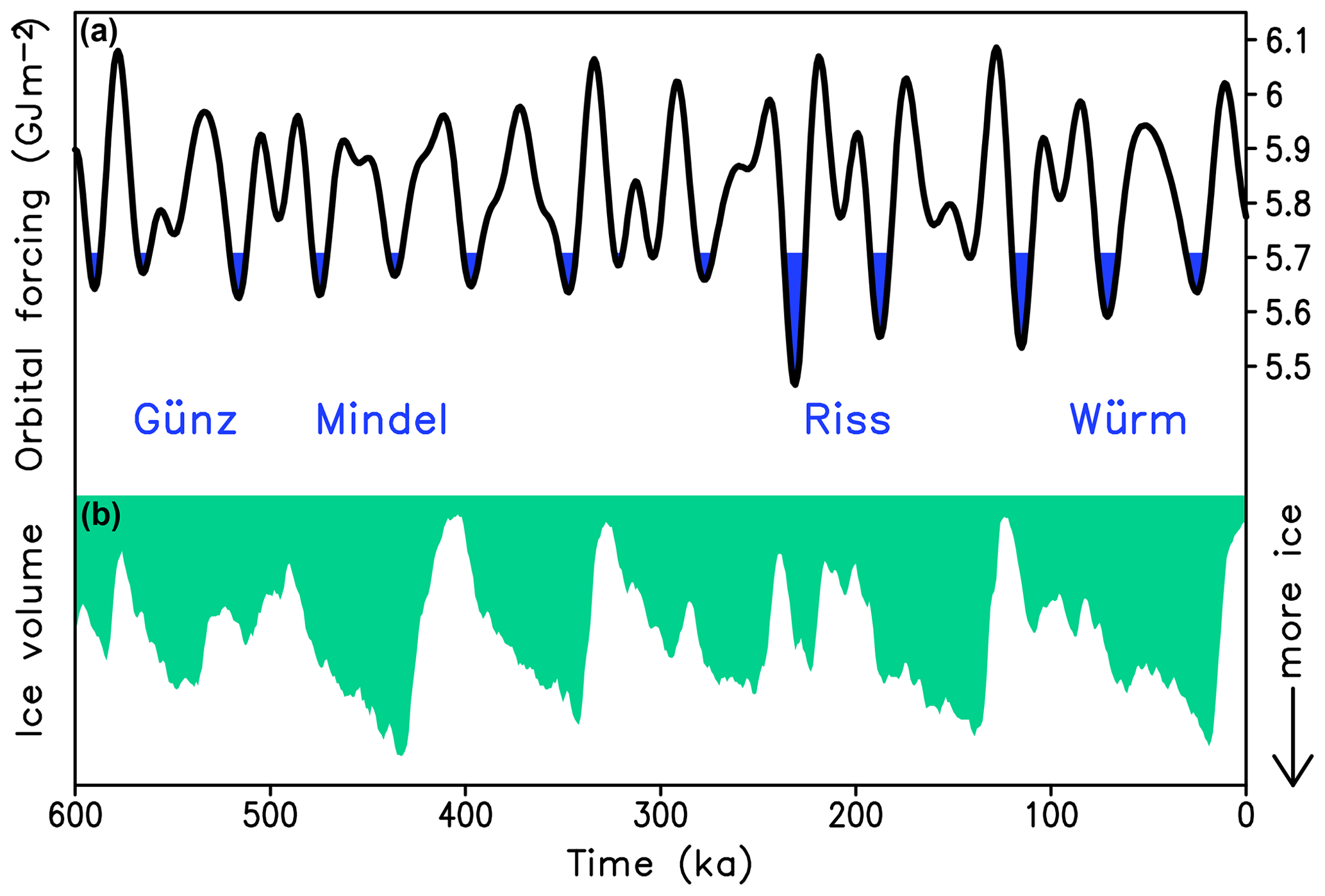
Figure 1Milankovitch forcing and ice volume variations over the past 600 kyr. (a) Caloric summer half-year insolation at 65∘ N. Blue shading represents insolation below 5.7 GJ m−2, the insolation threshold selected to match best Fig. 57 in Milankovitch (1941). According to the Milankovitch theory, glaciations occurred during periods of low insolation. The names of major glaciations, according to Penck and Brückner (1909), are written below the “Milankovitch curve”. (b) LR04 (Lisiecki and Raymo, 2005) benthic δ18O stack, a proxy for the global ice volume (inverted for convenience).
In Milankovitch's time, it was not known that the “glacial age” was the dominant mode of operation of the Earth system during the Quaternary. This is why Milankovitch considered ice ages to be the episodes that occurred during periods of low summer insolation. Although Milankovitch did not explicitly formulate his conceptual model of glacial cycles, the text and figures indicate that Milankovitch assumed that ice ages occurred during periods when caloric summer (half-years) insolation was below a certain threshold value (Fig. 1). Using a simple energy balance climate model, Milankovitch estimated that typical changes in summer insolation by 1000 canonical radiation units (1 canonical unit is approximately equal to 0.428 MJ) would cause 5 ∘C of summer cooling. Such cooling, in turn, is sufficient to lower the snow line by ca. 1 km and cause a widespread glaciation which is further amplified by the snow–albedo feedback. Thus, Milankovitch, for the first time, demonstrated that variations in insolation caused by astronomical factors are capable of driving glacial cycles. According to the Milankovitch conceptual model, three glaciations occurred during the last 120 kyr, which at the time of Milankovitch were known as Würm I, II, and III and now are usually notated as MIS 5d, 4, and 2. Although this was a significant step forward in explaining past glacial cycles, a comparison of the orbital forcing with the Earth system response shown in Fig. 2 reveals problems with the classical Milankovitch theory. It turned out that the Milankovitch conceptual model is more applicable to the 41 kyr world of the early Quaternary rather than the 100 kyr world of the late Quaternary.
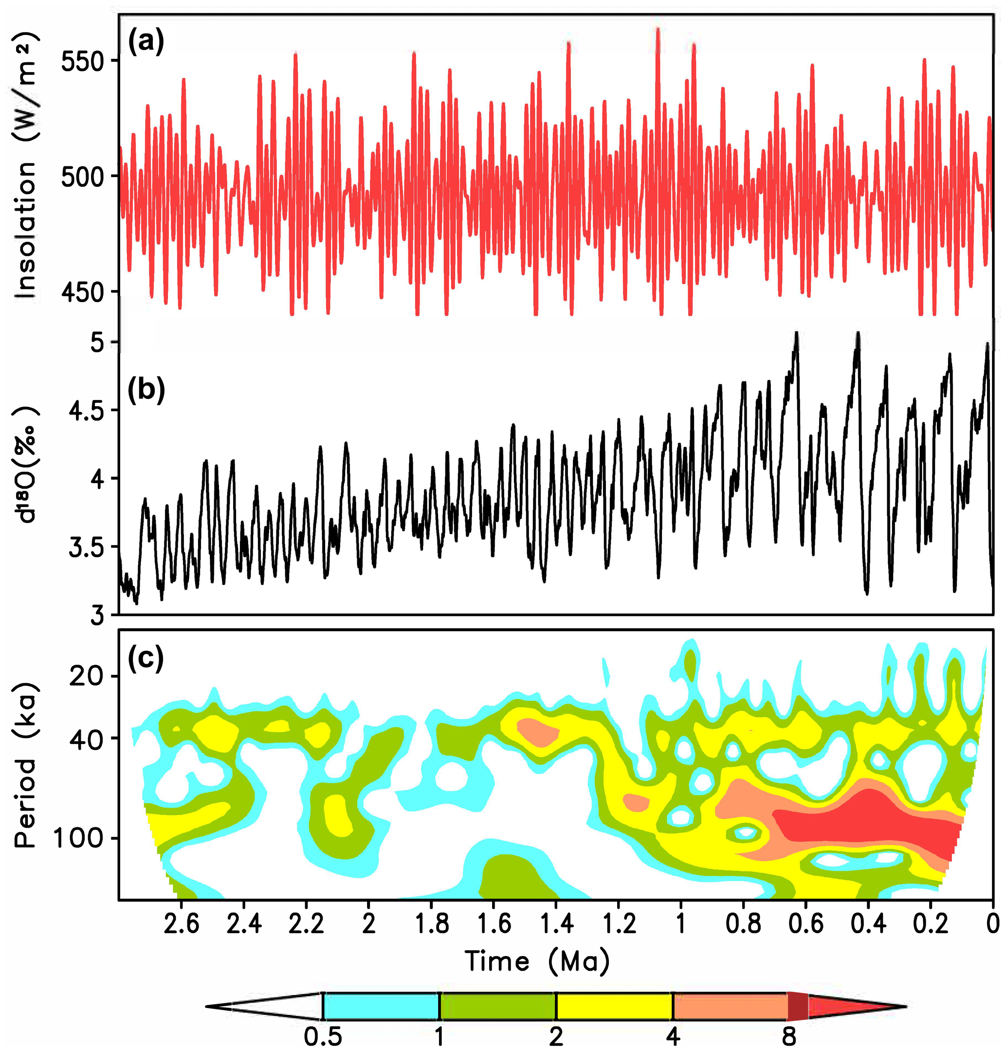
Figure 2Orbital forcing and the Earth system response during the entire Quaternary period. (a) Maximum summer insolation at 65∘ N computed using Laskar et al. (2004) orbital parameters; (b) LR04 (Lisiecki and Raymo, 2005) benthic δ18O stack, a proxy for global ice volume; (c) wavelet spectra of LR04 stack (in arbitrary units).
1.2 Testing Milankovitch theory with paleoclimate records
During the life of Milutin Milankovitch, no reliable paleoclimate records of glacial cycles existed to test his theory. Such records based on δ18O in marine sediments became available only during 1960s (Emiliani, 1966), and the first results of their analysis (e.g., Broecker and van Donk, 1970) provided strong support for the Milankovitch theory. Hays et al. (1976) demonstrated that the frequency spectra of planktic δ18O, considered a proxy for the global ice volume, contain both obliquity and precession frequencies, i.e., the frequencies of the Milankovitch insolation curves (Berger, 1976). However, the dominant periodicity of the recent glacial cycles was 100 kyr. This periodicity is absent in the spectrum of insolation but is close to one of the periodicities of eccentricity, which modulates the precession component of orbital forcing. In this landmark paper, the authors also demonstrated a close phase relationship between glacial cycles and eccentricity cycles and proposed that the 100 kyr cyclicity of the late Quaternary glacial cycles originates from a nonlinear climate response to eccentricity.
One of the most comprehensive attempts so far to test and extend Milankovitch theory beyond its original formulation was undertaken in the early 1990s by a large group of scientists (also known as the SPECMAP group after the project acronym) in two papers – Imbrie et al. (1992) and Imbrie et al. (1993). In the first one, it was concluded that 23 kyr (precession) and 41 kyr (obliquity) cycles seen in different paleoclimate records can be explained as a linear response of the climate system to insolation changes in high latitudes of the Northern Hemisphere. In the second paper devoted to the origin of 100 kyr cyclicity in the late Quaternary, the authors discussed several potentially important processes and climate feedbacks but did not arrive at a definite conclusion about the nature of 100 kyr cycles. The SPECMAP group acknowledged that these cycles could originate from the existence in the climate system of internal self-sustained oscillations with a similar periodicity, or, alternatively, 100 kyr cycles represent forced oscillations where the climate system acts as “a nonlinear amplifier which is particularly sensitive to eccentricity driven modulations in the 23 000-year sea level cycle” (Imbrie et al., 1993).
The nature of glacial cycles and Milankovitch theory attracted significant attention in the decades following SPECMAP publications, and numerous ideas of how to test and further develop Milankovitch theory have been proposed. First, the original Milankovitch theory has been turned from the theory of glacial ages into the theory of glacial terminations, and several studies analyzed whether the timing of glacial terminations is consistent with the Milankovitch theory in its new termination version (e.g., Huybers and Wunsch, 2005; Raymo, 1997). Second, instead of caloric half-year summer insolation used by Milankovitch, the June, July, or summer solstice insolation at 65∘ N became the standard metric for the orbital forcing (e.g., Berger, 1978). Defined this way, the orbital forcing became dominated by precession, while in the original Milankovitch version, the contributions of obliquity and precession were comparable. Third, Antarctic ice core analysis revealed significant variations in CO2 concentration, which closely followed 100 kyr cycles of global ice volume (Petit et al., 1999). This led to the appreciation of the importance of CO2 as the driver of glacial cycles and thus to the merging of the Milankovitch and Arrhenius theories, which before were considered to be alternative theories of glacial cycles (e.g., Ruddiman, 2003).
1.3 Testing Milankovitch theory with models
With the development of climate and ice sheet models, efforts to test the validity of the Milankovitch theory also began on the modeling front. The impact of Earth orbital parameter changes was first investigated with atmospheric models (e.g., Kutzbach, 1981). It had been shown that surface air temperature and atmospheric dynamics (e.g., summer monsoons) are strongly affected by orbital parameter changes. Over the past 20 years, several “time slices” (mid-Holocene and the Eemian interglacial) have received special attention in the framework of paleoclimate intercomparison projects (e.g., Braconnot et al., 2007). Results of these studies confirmed the strong influence of orbital forcing on climate even though changes in Earth's orbital parameters have little effect on global annual mean insolation. It is noteworthy that a typical sensitivity of summer temperature over the Northern Hemisphere land to orbital forcing (about 1 ∘C per 10 W m−2) found in climate model simulations is rather similar to the original Milankovitch estimate. Thus, the first premise of the Milankovitch theory of ice ages, namely that changes in insolation caused by variations of the Earth's orbital parameters strongly affect climate, had been confirmed.
The next step in testing the Milankovitch theory was modeling climates favorable for glacial inception. The aim was to verify whether the cooling caused by the lowering of boreal summer insolation is sufficient to trigger large-scale Northern Hemisphere glaciation (“ice age”). Since the last glacial cycles began around 115 ka, the time when boreal summer insolation was about 10 % lower than at present, most such experiments have been performed for this time. Simulations with different climate models show pronounced summer cooling over continents in the Northern Hemisphere. However, as far as the glacial inception (the build-up of ice sheets) was concerned, the results were rather ambiguous: some models simulated the appearance of perennial snow cover at least in several continental grid cells, while others did not (e.g., Royer et al., 1983; Dong and Valdes, 1995; Varvus et al., 2008). This ambiguity is not surprising since the magnitude of climate biases in model simulations is often comparable to models' responses to orbital forcing. In addition, a rather coarse spatial resolution of climate models used in these studies does not allow resolving topographic details, which may be critical for the appearance of ice sheet nucleation centers (Marshall and Clarke, 1999). In any case, without coupling climate models to ice sheet models, it was impossible to determine whether the simulated climate response to orbital forcing was consistent with the observed ice volume growth rate.
Simulations of glacial cycles with simple ice sheet models began in the 1970s with 1-D models (e.g., Weertman, 1976; Oerlemans, 1980; Pollard, 1983). The latter study produces rather impressive agreement between modeled and reconstructed ice volume. It also demonstrated the importance of the delayed isostatic rebound and what is now called marine ice sheet instability (MISI) for the realistic simulation of glacial cycles. Later, the complexity and spatial resolution of both climate and ice sheet modeling components increased, which allowed simulating the temporal evolution of ice sheets during the past glacial cycles and comparing them with available paleoclimate reconstructions (e.g., Tarasov and Peltier, 1997; Berger et al., 1999; Zweck and Huybrechts, 2003).
More recently, a new class of models, Earth system models of intermediate complexity (EMICs, Claussen et al., 2002), have been used for long transient simulations of the glacial cycles, first with prescribed GHG concentrations (e.g., Charbit et al., 2007; Ganopolski et al., 2010; Heinemann et al., 2014; Choudhury et al., 2020) and finally with the fully interactive carbon cycle (Ganopolski and Brovkin, 2017; Willeit et al., 2019). The latter study also succeeded in simulating the mid-Pleistocene transition from the 41 to 100 kyr world. One of the important results obtained with EMICs was the demonstration of the existence of multiple equilibria states in the phase space of the orbital forcing and that the glacial inception represents a bifurcation transition from one state to another (Calov and Ganopolski, 2005). Only recently have transient simulations with ice sheet models coupled to GCMs become possible, but so far, such simulations have been restricted to modeling only glacial inception (Gregory et al., 2012; Tabor and Poulsen, 2016; Lofverstrom et al., 2022).
Conceptual models of glacial cycles can be defined as a set of formal rules or mathematical operators that translate a certain metric for orbital forcing (usually boreal summer insolation) into quantitative or qualitative information about the temporal dynamics of glacial cycles. Despite progress with the modeling of glacial cycles using a process-based model, conceptual models remain a popular tool for studying the mechanisms of glacial cycles.
2.1 Qualitative conceptual model of glacial cycles
The term “qualitative” here is applied to models that do not simulate the temporal evolution of climate characteristics but instead provide only qualitative information about glacial cycles. The first model of this sort was proposed by Joseph Adhémar, the author of the first astronomical theory of ice ages. He proposed that ice ages were caused by long winters and occurred with the periodicity of the precession of the equinox, i.e., ca. 23 000 years (Adhémar, 1842). James Croll later changed long to cold winters as the precondition for hemispheric glaciations (Croll, 1864). In turn, Milutin Milankovitch adopted the view that glaciations occurred during “cold summers”. In a quantitative form, Milankovitch's theory of glacial ages (see Fig. 1, which is similar to Fig. 48 from Milankovitch, 1941) can be formulated as follows: ice ages occur when summer insolation drops below a certain threshold value.
Among examples of more recent qualitative conceptual models of glacial cycles is the idea that glaciations are triggered by every fourth or fifth precession cycle after “unusually low” summer insolation maxima (Raymo, 1997; Ridgwell et al., 1999). This conceptual model closely relates glacial cycles to the eccentricity cycles since unusually low summer insolation maxima occur during periods of low eccentricity. An alternative conceptual model in which precession plays no role was proposed by Huybers and Wunsch (2005). According to this model, glacial terminations of the late Quaternary were spaced in time with equal probability by two or three obliquity cycles without any relation to other orbital parameters (see also Appendix A3). More recently, Huybers (2011) also accounted for the role of precession in pacing glacial cycles and proposed a conceptual mathematical model where the timing of glacial termination is controlled by a metric of orbital forcing similar to Milankovitch's caloric half-year insolation.
Recently, Tzedakis et al. (2017) proposed a rule which relates the timing of glacial terminations to the original Milankovitch metric for the orbital forcing, namely half-year caloric summer insolation. Tzedakis et al. (2017) found that glacial terminations during the late Quaternary occurred when the “effective energy” (a function of caloric half-year insolation and elapsed time since the previous termination) exceeds a certain value. This conceptual model and its relationship to GMT are discussed in Appendix A3.
2.2 Mathematical conceptual models of glacial cycles
Mathematical conceptual models of glacial cycles are based on one or several equations that describe climate system response to orbital forcing. Usually, the state of the climate system is expressed through the global ice volume (e.g., Imbrie and Imbrie, 1980; Paillard, 1998), but some models also include equations for CO2 concentration and temperature (e.g., Saltzman and Verbitsky, 1993; Saltzman, 2002; Paillard and Parrenin, 2004; Talento and Ganopolski, 2021) or some dynamical properties of the ice sheets (e.g., Verbitsky et al., 2018). Orbital forcing in such models is represented by a function of Earth's orbital parameters, usually by the maximum summer insolation at 65∘ N, caloric half-year insolation, or similar characteristics. Conceptual models of glacial cycles can be divided into “inductive” models (like Imbrie and Imbrie, 1980; Paillard, 1998) where governing equations were selected to produce an output close to the paleoclimate records and models where the equations were derived with some assumptions and simplifications from the basic equations describing dynamics of climate and ice sheets (e.g., Tziperman and Gildor, 2003; Verbitsky et al., 2018). The third type of conceptual models, namely models derived using the results of complex Earth system models, is described in the next section.
Calder (1974) and Imbrie and Imbrie (1980) proposed the first models of this type. Both models simulate global ice volume evolution in response to boreal summer insolation variations. While Calder's model simulates glacial cycles, which is dominated by precession and obliquity and has too little energy in the frequency spectra for the 100 kyr periodicity, the Imbrie and Imbrie model (see also Appendix A2) has too much energy in the 400 kyr band, which is another eccentricity periodicity (see also Paillard, 2001). These problems are typical for many conceptual models. An important step in developing conceptual models of glacial cycles was made by Paillard (1998) (P98 hereafter). This model is similar to the Imbrie and Imbrie model, but it additionally postulates the existence of different equilibrium states and different regimes of operation, including a fast regime of deglaciation which occurs after reaching a critical ice volume. The idea of such catastrophic behavior of ice sheets after reaching some critical state was probably first proposed by MacAyeal (1979). This strong nonlinearity enables the model to achieve very good agreement with paleoclimate reconstructions and, in particular, to eliminate the 400 kyr peak in the frequency spectra of ice volume. The P98 model has played a critical role in the development of GMT and will be discussed in more detail in the forthcoming sections.
Admittedly, a number of other conceptual models simulate past glacial cycles with reasonable skill. In many of them, glacial cycles represent self-sustained oscillations with superimposed Milankovitch cycles (see Roe and Allen, 1999, and Crucifix, 2012, for an extensive discussion and comparison of different conceptual models). These studies also revealed that many models produce similarly good agreement with the empirical data despite very different assumptions and formulations. Roe and Allen (1999) concluded the following.
We find there is no objective evidence in the record in favour of any particular model. The respective merits of the different theories must therefore be judged on physical grounds.
To explain this apparent paradox, a “minimal” model of glacial cycles is described in the next section. The simplicity of the recipes needed to simulate “realistic” glacial cycles explains why different conceptual models produce similar results.
2.3 “Minimal” conceptual models of glacial cycles
One of the main challenges in modeling the late Quaternary glacial cycles is the dominant 100 kyr periodicity (a single sharp peak in the frequency spectra at the period close to 100 kyr) and the absence of the energy maximum at 400 kyr, which is another eccentricity period. While the linear transformation of orbital forcing would not show any significant energy at eccentricity periods, nonlinear transformations (like Imbrie and Imbrie model, see Appendix A2) contain all eccentricity periodicities. The simplest way to solve this problem is to design a model which possesses self-sustained oscillations with a periodicity close to 100 kyr and where orbital forcing plays a secondary role, namely the role of a pacemaker of long glacial cycles. Such a model with appropriate parameter choices can simulate glacial cycles with the correct frequency spectrum and timing of individual glacial cycles. Furthermore, such a model can be very simple and described by a single equation:
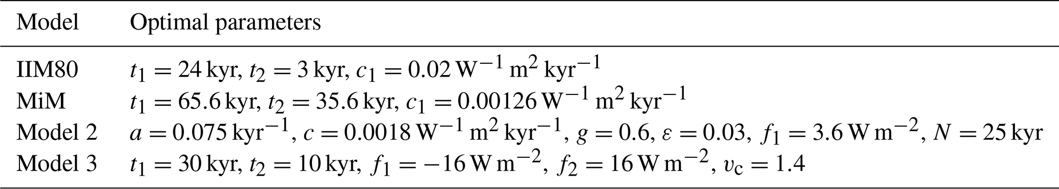
where v is the ice volume in arbitrary nondimensional units, time t is in kiloyears, ak and b are model parameters, and orbital forcing where F is the maximum summer insolation at 65∘ N and Fa is the average value of F over the last million years. The model has two “regimes”: k=1 corresponds to the period of ice growth and positive , while k=2 corresponds to ice decay and therefore negative . The transitions from the regime k=1 to k=2 occur when v=1 and from k=2 to k=1 when v=0. In the absence of orbital forcing, the solution involves sawtooth-like oscillations with the period . By proper choice of t1 and t2, this periodicity can be set to 100 kyr (Table 1). This is the minimal (MiM) model of glacial cycles which is similar to but even simpler than the model described in Leloup and Paillard (2022). This model has only three free parameters. For their optimal values given in Table 1, the model can achieve rather good agreement with the benthic δ18O record (Lisiecki and Raymo, 2005) with a correlation coefficient of 0.81 for the last 800 kyr (Fig. 3). Notably, the model solutions for the last 800 kyr strongly depend on the choice of model parameters but do not depend on the initial condition if the simulations begin from v=0 not later than 1000 kyr before present. The model described by Eq. (1) is the simplest version of the relaxation oscillator, which is phase-locked to orbital forcing. Many other conceptual models have more complex formulations but in terms of dynamics are essentially identical to the model described by Eq. (1).
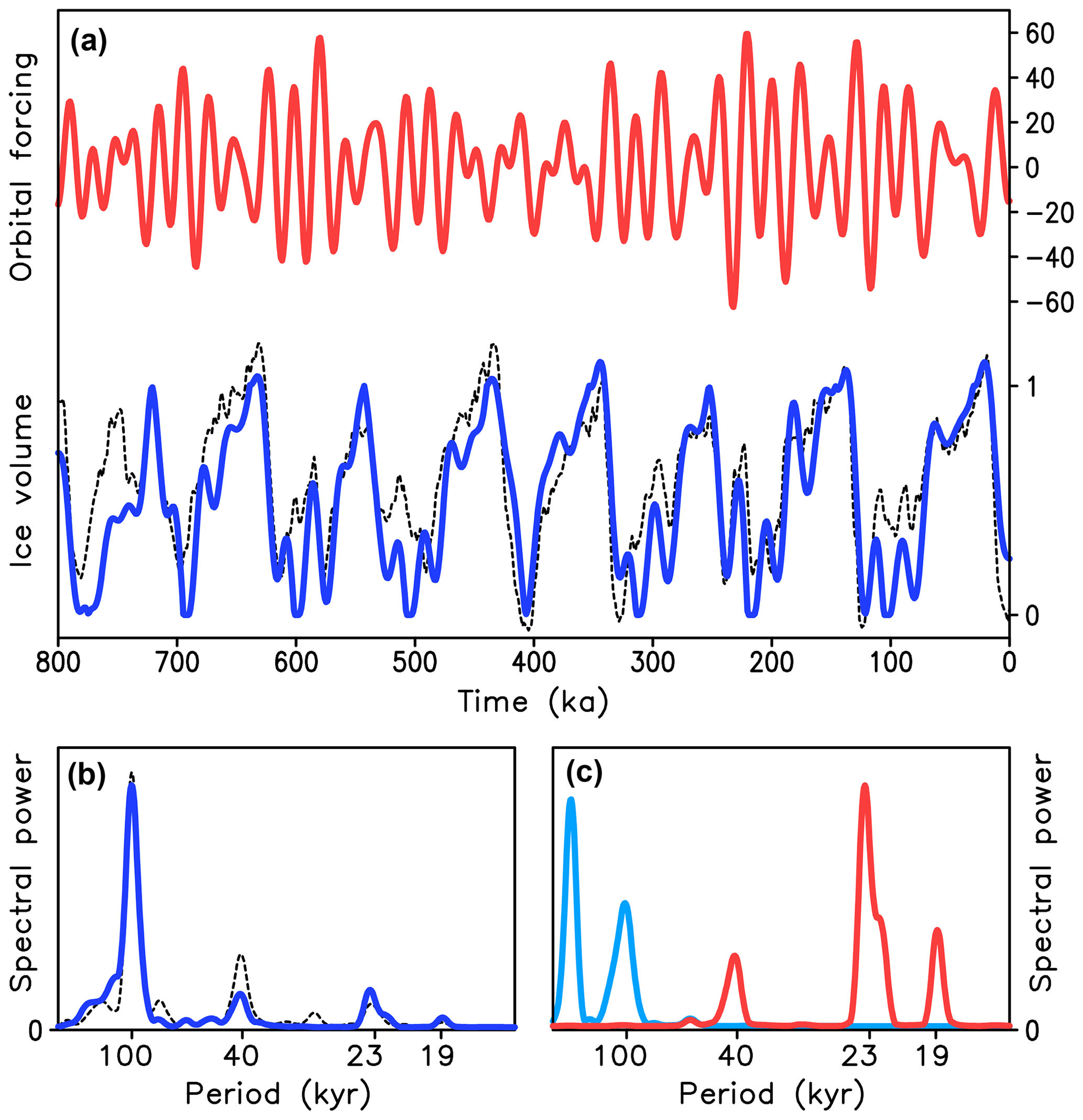
Figure 3Simulations of late Quaternary glacial cycles with the “minimal” conceptual model MiM. (a) Orbital forcing (maximum summer insolation at 65∘ N) and (b) results of MiM versus paleoclimate reconstruction. The solid lines are modeling results, and the dashed line is an arbitrarily scaled LR04 δ18O stack. (c) Frequency spectra of MiM in comparison with the frequency spectra of LR04 stack. (d) Frequency spectra of orbital forcing (red) and eccentricity (blue).
What can be learned from this simple modeling exercise? Obviously, it demonstrates that it is very easy to design a simple model (mathematical transformation) which converts orbital forcing into the benthic δ18O-like curve for the last 800 kyr with sufficiently good accuracy. These recipes are the following. First, the model has to possess two regimes: slow ice growth and fast deglaciation regimes. Second, the transitions between the first and the second regimes should occur after some critical ice volume is reached. Third, the time needed to reach this critical ice volume should be about 100 kyr. What remains to be explained is
-
why the Earth system during the Quaternary behaves like a relaxation oscillator;
-
what the physical meaning of the “critical ice volume” is and why reaching critical volume leads to regime change and deglaciation;
-
why deglaciation is much shorter than the phase of predominant ice sheet growth;
-
whether the Earth system possesses an internal timescale close to 100 kyr or this timescale is directly related to the eccentricity.
These and other questions will be discussed in Sect. 4. In the next section, a new conceptual model will be introduced and used to illustrate a number of essential aspects of GMT.
3.1 Modeling concept
As shown above, even a very simple conceptual model can simulate global ice volume evolution in good agreement with the reconstructed one. The reason why a new conceptual model is presented here is not that it has a better performance than other models of the same class but because it is based on the results of a process-based Earth system model, CLIMBER-2. In turn, it has been shown that CLIMBER-2 can successfully simulate Quaternary glacial cycles using orbital forcing as the only external forcing (Willeit et al., 2019). Thus, this new conceptual model is fundamentally different by design from other conceptual models.
The development of a new conceptual model has been done in two steps. First, based on the analysis of CLIMBER-2 model results (considered hereafter as Model 1), a simple but still physically based reduced-complexity model (Model 2) has been designed. This model is described in Appendix A4. A three-equation version of this model was used in Talento and Ganopolski (2021). Model 2 has then been additionally simplified, and in this way Model 3 was designed. This model is described below.
The key results of CLIMBER-2, which have been obtained in Calov and Ganopolski (2005), Ganopolski and Calov (2011), and Willeit et al. (2019), used to design Models 2 and 3 are the following.
-
The mass balance of ice sheets strongly correlates with the maximum summer insolation at 65∘ N.
-
The existence of multistability of the climate–cryosphere system in the phase space of orbital forcing with the bifurcation transitions between different states.
-
The typical (relaxation) timescale of the climate–cryosphere is about 20–40 kyr.
-
Robustness of simulated glacial cycles regarding the choice of initial conditions and model parameters.
-
Phase locking of the late Quaternary glacial cycles to the 100 kyr eccentricity cycle.
-
Strong asymmetry between ice sheet growth phase and glacial terminations.
Model 3 does not explicitly account for the role of CO2 in glacial cycles, which was analyzed in previous studies (e.g., Ganopolski and Calov, 2011; Ganopolski and Brovkin, 2017). For the sake of simplicity, it is assumed here that the role of CO2 is implicitly represented by ice volume since these two characteristics are highly correlated. The role of CO2 in shaping glacial cycles will be discussed in the next section.
3.2 Model 3 formulation
The new conceptual model of glacial cycles (Model 3) is based on the existence of multiple equilibrium states found in Calov and Ganopolski (2005) and reproduced by Model 2 (see Appendix A4). The first (interglacial) state is characterized by a warm climate and the absence of continental ice sheets in the Northern Hemisphere. The second one, with the ice sheets covering significant fractions of North America and Eurasia, is the glacial state. In the framework of this concept, the evolution of the Earth system under the influence of orbital forcing is described as the relaxation towards the corresponding equilibrium state. Model 3 contains only one variable – global ice volume v (in nondimensional units), described by the following equation:
with the additional constraint v≥0. Equation (2) describes two different regimes of ice sheet evolution. The first one (k=1), similar to the P98 model, is the glaciation regime when the system relaxes toward the equilibrium glacial state Ve with the timescale t1. The second regime (k=2) is the deglaciation regime when ice volume linearly declines toward zero with the characteristic timescale t2, with vc being the model parameter that defines the critical ice volume (see below). The equilibrium state Ve towards which the system is attracted is a function of orbital forcing and, for the bi-stable regime, also depends on ice volume (see Fig. 4a):
The glacial equilibrium state is defined as
The unstable equilibrium which separates the glacial and interglacial attraction domains is defined as
and the interglacial equilibrium Vi=0. Here orbital forcing f (in W m−2), similar to the minimal conceptual model MiM, is defined as , where F is the maximum summer insolation at 65∘ N, Fa is its averaged value over the last million years, and f1 and f2 are model parameters. Note that orbital forcing only enters Eq. (2) in a parametric form. Unlike Model 2, from which it was derived, Model 3 does not explicitly include positive and negative feedbacks, but the existence of such feedbacks determines the shape of the stability diagram of Model 3 (Fig. 4), which is the same as for Model 2 (Fig. A4). The only qualitative difference between Models 2 and 3 is that in the latter, the relaxation timescales are fixed, while in the former, they depend on the position in phase space of orbital forcing and ice volume. This explains the very close similarity of the trajectories in this phase space (compare Figs. 4b and A4b).
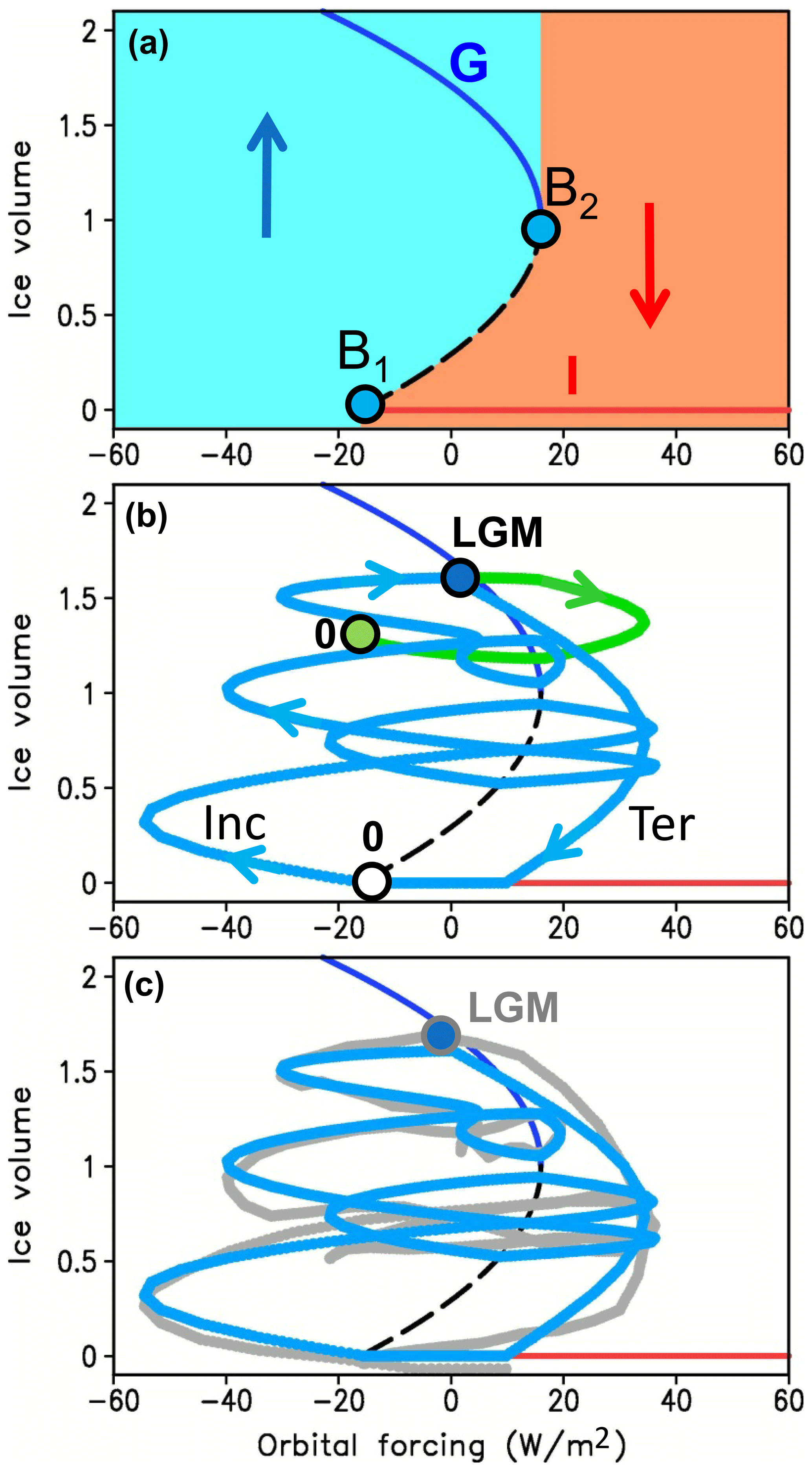
Figure 4Evolution of the modeled ice volume in the phase space of orbital forcing. (a) Two equilibrium solutions: G – glacial, I – interglacial. The blue area is the attraction domain of the glacial state, the red area is the attraction domain of the interglacial state, and the dashed line is an unstable solution separating the two domains. B1 and B2 are the bifurcation points, and B1 corresponds to glacial inception. This diagram corresponds only to the glaciation regime. For the deglaciation regime, there is only one equilibrium state – I. (b) Evolution of simulated ice volume (nondimensional) during the past glacial cycle starting at time 120 ka. “Inc” denotes glacial inception, and “Ter” indicates glacial terminations. Note that after the LGM (20 ka) the model without a termination regime (green line) failed to deglaciate. (c) Comparison of model simulation with LR04 benthic δ18O stack.
The transition from a glacial (k=1) to deglaciation regime (k=2) occurs if three conditions are met: v>vc, , and f>0. The transition from deglaciation to glacial regime occurs if orbital forcing f drops below the glaciation threshold f1. The interglacial state formally belongs to the deglaciation regime.
The model has five parameters (t1, t2, f1, f2, vc), all of which, in principle, can be used to maximize the agreement between simulated and reconstructed ice volume. However, all these parameters have clear physical meaning and can be directly estimated using the results of CLIMBER-2 and paleoclimate data. The value of f1 (insolation threshold for glacial inception) was rather tightly constrained by the current insolation minimum ( W m−2) when glaciation did not occur and MIS 19 insolation minimum ( W m−2) when it did occur (Ganopolski et al., 2016). According to Calov and Ganopolski (2005), the relaxation timescale t1 is about 30 kyr, and f2 is positive. It is noteworthy that model results depend on a combination of t1 and f2, and essentially identical solutions can be obtained for different combinations of these two parameters. Deglaciation timescale t2 derived from the model and paleoclimate records is about 10 kyr. The last model parameter, the critical ice volume vc, controls the dominant periodicity and degree of asymmetry of glacial cycles. As a result, only f2 and vc were used as tunable parameters and their values (Table 1) have been chosen to maximize the correlation between simulated ice volume and the benthic δ18O record (LR04) during the past 800 kyr. The δ18O has been used here as the ice volume proxy even though several reconstructions of sea level for the last 800 kyr exist (i.e., Spatt and Lisiecki, 2016). This has been done to enable the comparison of model results with the paleoclimate data for the entire Quaternary. Such a choice is justified by a strong similarity between the LR04 stack and late Quaternary sea level reconstructions. Model 3 is similar to the P98 model by formulation and its results, but it does not contain timescales close to 100 kyr.
3.3 Simulation of the late Quaternary glacial cycles with Model 3
Results of model simulations depicted in Fig. 5 show good agreement with the LR04 stack for the last 800 kyr. The correlation between the model and data is 0.85 for the entire time interval. The agreement is better for the later part (the correlation is 0.9 when only considering the last 400 kyr) than for the earlier part, which can be partly explained by the fact that the model and LR04 are in antiphase around 700 and 490 kyr. Since LR04 has been tuned to the Imbrie and Imbrie model, which has a very strong precession component, the cause of such a large data–model mismatch is unclear. The frequency spectrum of the model results in good agreement with paleodata has a dominant sharp 100 kyr maximum, with little energy in the 400 kyr band and a relatively weak precession component compared to the spectrum of orbital forcing (Fig. 5c). Simulated glacial cycles are rather insensitive to the initial conditions since they converge rapidly to the common solution (Fig. 6c). This agrees with CLIMBER-2 simulations (Willeit et al., 2019) where we concluded that “simulated glacial cycles only weakly depend on initial conditions and therefore represent a quasi-deterministic response of the Earth system to orbital forcing”. Modeling results are also robust regarding the choice of model parameters. For example, when keeping other model parameters constant, as in Table 1, essentially the same results are obtained for the range of vc between 1.32 and 1.49 (Fig. 6b). It is noteworthy that, although Model 3 is based on CLIMBER-2 and aimed to mimic it, Model 3 actually outperforms the CLIMBER-2 model in terms of the agreement with empirical data for the last 800 kyr. In particular, CLIMBER-2 has a problem with simulating the correct timing of Termination V prior to MIS 11 (see Willeit et al., 2019), while Model 3 does not have such a problem.
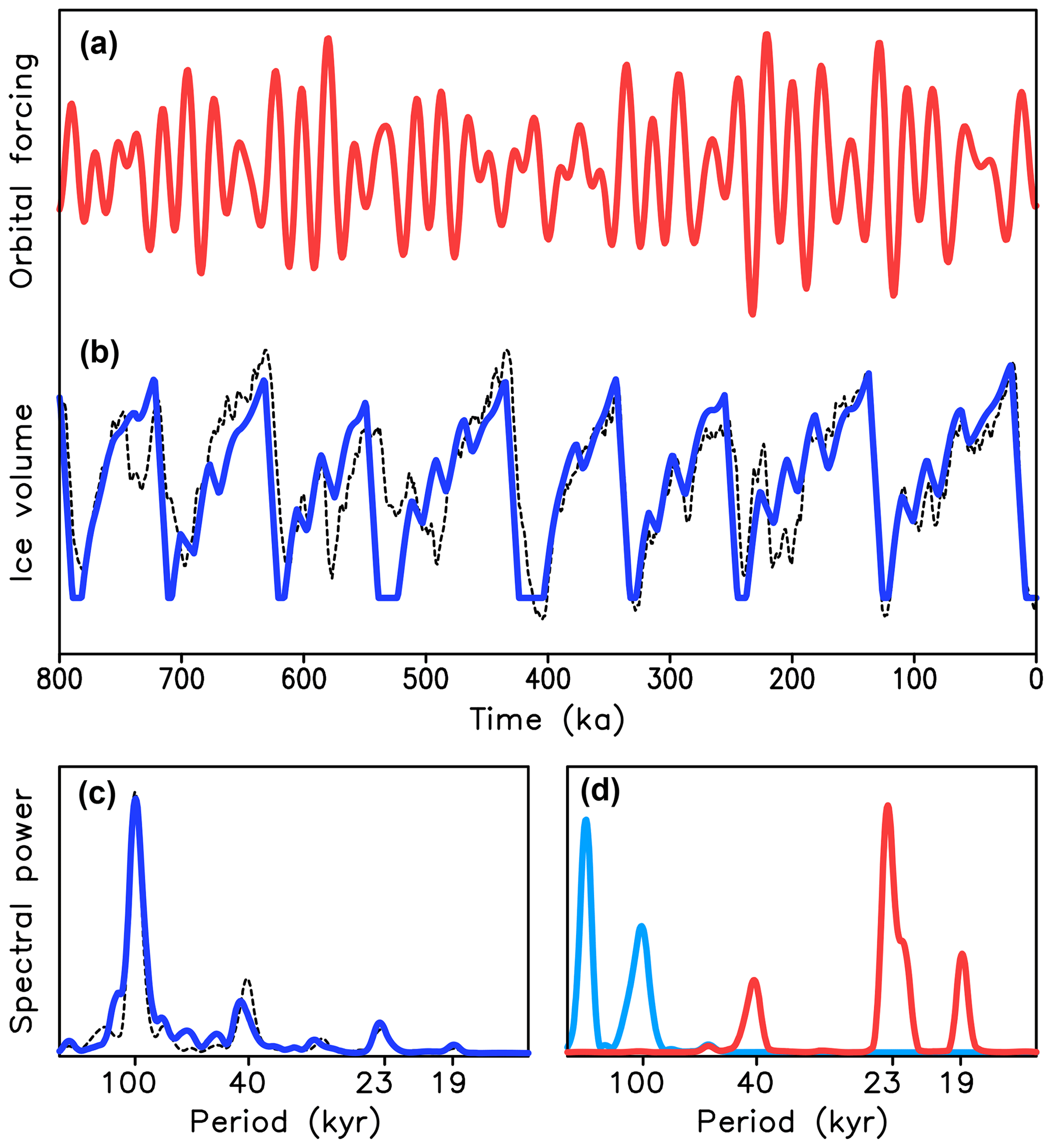
Figure 5Results of simulations of the last 800 kyr with conceptual Model 3. (a) Orbital forcing; (b) simulated ice volume in nondimensional units (blue) and scaled LR04 stack (dashed line); (c) spectra of simulated ice volume (blue) and LR04 stack (dashed line); (d) frequency spectra of the orbital forcing.
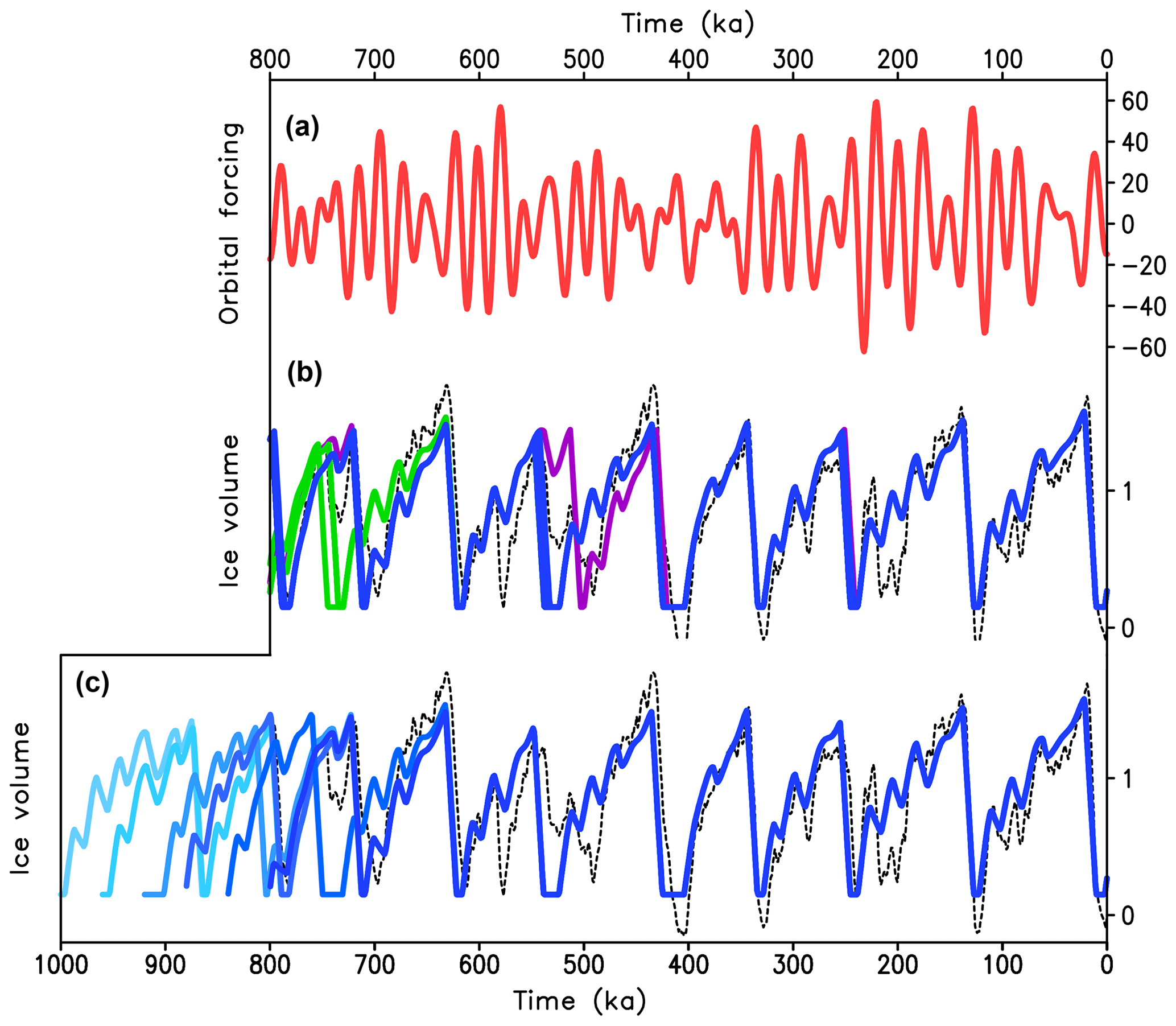
Figure 6Results of simulations of the last 800 (1000) kyr with conceptual Model 3. (a) Orbital forcing; (b) simulated ice volume (green lines correspond to the range of vc 1.32–1.38, blue to the range 1.39–1.48, purple to vc=1.49). Thus, the timing of most glacial terminations (and all the latest five) coincides for the broad range of vc from 1.32 to 1.49. (c) Simulated ice volume for vc=1.4 (different colors correspond to different starting times from 1000 to 800 ka with the step 40 ka). All runs converge to the same solution after less than 200 kyr. Note the similarities with Fig. 6b from Ganopolski and Calov (2011). (b, c) The LR04 stack is shown by dashed lines.
The existence of two regimes of operation is postulated in Model 3 similarly to P98, and it is absolutely critical for simulating realistic glacial cycles. To demonstrate this, an additional experiment has been performed with Model 3 but without the termination regime. This experiment started from v=0 at 125 ka (Eemian interglacial) and was run to present day. The trajectory of ice volume evolution in the phase space of orbital forcing for this experiment is compared with the standard Model 3 in Fig. 4b. The two model versions are identical before 20 ka when the termination regime is activated in the standard model version. If the termination regime is disabled, the model trajectory in the phase space represents a loop similar to previous precession cycles (green line) and does not result in deglaciation. This result does not depend on the choice of model parameters, and there are no combinations of model parameters that enable the simulation of the realistic glacial cycles without the termination regime.
3.4 Generic orbital forcing and the origin of 100 kyr cyclicity in Model 3
In Ganopolski and Calov (2011) we argued that the “100 kyr peak in the power spectrum of ice volume results from the long glacial cycles being synchronized with the Earth's orbital eccentricity”. To understand how this synchronization occurs, Model 3 was forced by a generic orbital forcing instead of the real summer insolation. This generic forcing consists of a periodic precession-like harmonic component with a single periodicity of 23 kyr, with the amplitude modulated by schematic eccentricity-like cycles with a periodicity of 100 kyr:
where A is the magnitude of forcing in W m−2 and ε is the nondimensional magnitude of amplitude modulation.
The first experiment is performed with the simplest periodic orbital forcing with A=25 W m−2 and ε=0. Figure 7 shows model results for three values of the critical ice volume: vc=1.2, 1.33, and 1.47. The model simulates periodic glacial cycles with the amplitudes and periods increasing with vc. Naturally, these periods are multiples of 23 kyr. For vc=1.2 this period is equal to kyr, and for vc=1.47 the period is kyr; only for vc=1.33 is the period kyr relatively close to 100 kyr (Fig. 7c). Note that all these periods are much longer than the relaxation timescale of the model equal to 30 kyr.
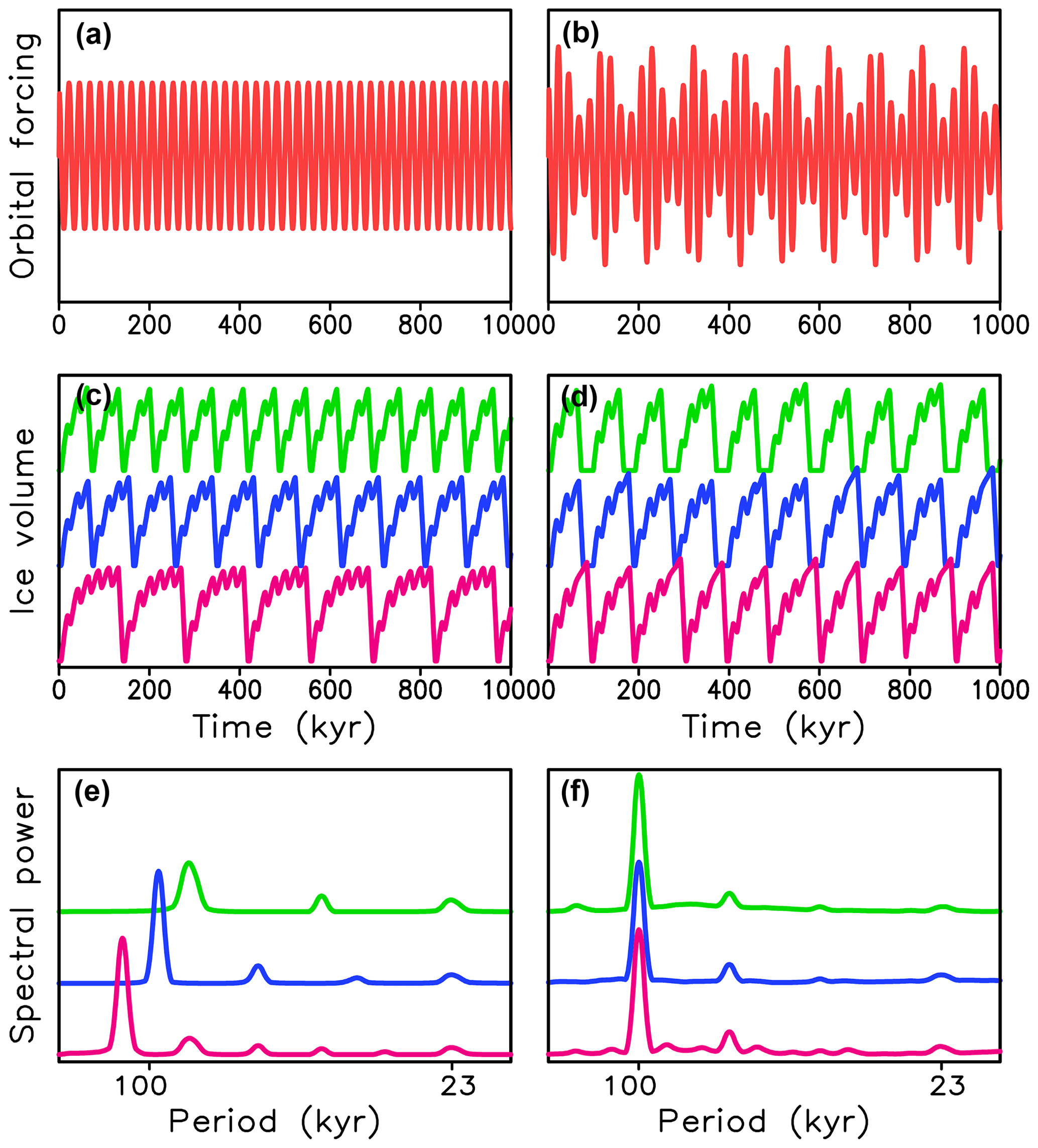
Figure 7Simulation of glacial cycles with Model 3 for different artificial orbital forcings. (a, b) Forcings, (c, d) simulated volume in arbitrary units. (e, f) Frequency spectra of simulated ice volume. (a, c, e) Periodic forcing with A=25 W m−2 , T=23 kyr, and ε=0 (Eq. 3). (b, d, f) Periodic forcing with additional 100 kyr amplitude modulation (ε=0.5). Green lines correspond to vc=1.2, blue – vc=1.33, purple – vc=1.47.
Applying amplitude modulation (ε=0.5) with a periodicity of 100 kyr to this generic forcing leads to quasiperiodic cycles with a sharp peak at 100 kyr in the frequency spectrum and similar timings of glacial terminations for all three values of critical ice volume (Fig. 7b, d and f). This is because, irrespective of the value of vc, all simulated cycles are phase-locked to the amplitude modulation cycle. This result is very robust with respect to the vc value and the amplitude and period of precession-like cycles, as well as to the amplitude and periodicity of the amplitude modulation cycle. Similarly, setting the periodicity of precession-like cycles in the range of 10 to 30 kyr has a minimal impact on the results (not shown).
The mechanism of the phase locking of long glacial cycles to the 100 kyr amplitude modulation cycle in the case of the generic orbital forcing is rather straightforward. After ice volume v exceeds a value of about 0.2 vc, the system stays longer in the attraction domain of the glacial state (see Fig. 4). Moreover, the smaller the amplitude of orbital forcing, the longer it stays in the attraction domain of the glacial state when ice is growing. Thus, the likelihood of reaching the critical ice volume vc is higher during periods of weak orbital forcing, i.e., during periods of low eccentricity. It is also noteworthy that the amplitude of simulated glacial cycles and the height of 100 kyr peaks in the frequency spectrum of ice volume (Fig. 7) are essentially independent of the magnitude of amplitude modulation in a wide range of parameter ε values.
3.5 Is the spectrum of ice volume variability consistent with the phase locking of glacial cycles to eccentricity?
While the formal relationship between eccentricity and late Quaternary glacial cycles has already been established in Hays et al. (1976), some studies (e.g., Muller and MacDonald, 1997; Maslin and Brierley, 2015) argued against the direct link between the 100 kyr cyclicity of glacial cycles and eccentricity. It is known that the direct effect of eccentricity on global insolation is negligibly small (e.g., Paillard, 2001), and this is why the eccentricity can affect climate only through the amplitude modulation of the precession cycle. In principle, the response of any nonlinear system to the forcing, which consists of a quasiperiodic carrier with amplitude modulated by another quasiperiodic signal, should contain periodicities of both carrier and amplitude modulation signal. However, eccentricity also has a strong 400 kyr periodicity which is practically absent in the late Quaternary ice volume reconstructions. In addition, the peak in the eccentricity spectrum near 100 kyr is split into two peaks at 95 and 124 ka, while the spectrum of the reconstructed ice volume contains very little energy at 124 kyr.
Results of the Imbrie and Imbrie model apparently support this critique since the spectrum of their model reveals all problems mentioned above: the low-frequency part of its spectrum is essentially identical to the spectrum of eccentricity (Fig. 8d) and very different from the δ18O spectrum for the last 800 kyr (Fig. 3). However, it is possible to construct a mathematical transformation that converts orbital forcing into realistic ice volume evolution, and Model 3 is an example of such transformation (Fig. 5). To enhance the resolution of the frequency spectrum, the model has been run through the past 3 Myr with the fixed model parameters. Only the last 2.8 were analyzed and are shown in Figs. 8 and 9. Unsurprisingly, the model with parameters tuned to the 100 kyr world cannot reproduce the 41 kyr world, and simulated glacial cycles are realistic only for the last million years. Unlike the Imbrie and Imbrie model, the spectrum of Model 3 does not contain a 400 kyr peak and has a single sharp peak at 95 kyr (Fig. 8d). Such behavior is robust for a wide range of model parameters, for example for vc in the range between 1.2 and 1.5. The absence of 400 kyr periodicity in the frequency spectra of Model 3 can be explained by the fact that each glacial termination “erases” the system memory, and the amplitude of the next glacial cycle does not depend on the previous one. The main reason why the spectrum of Model 3 is so different from the spectrum of eccentricity is because the eccentricity is not the forcing of glacial cycles, but rather a pacemaker that sets the dominant periodicity and, to some degree, the timing of glacial terminations.
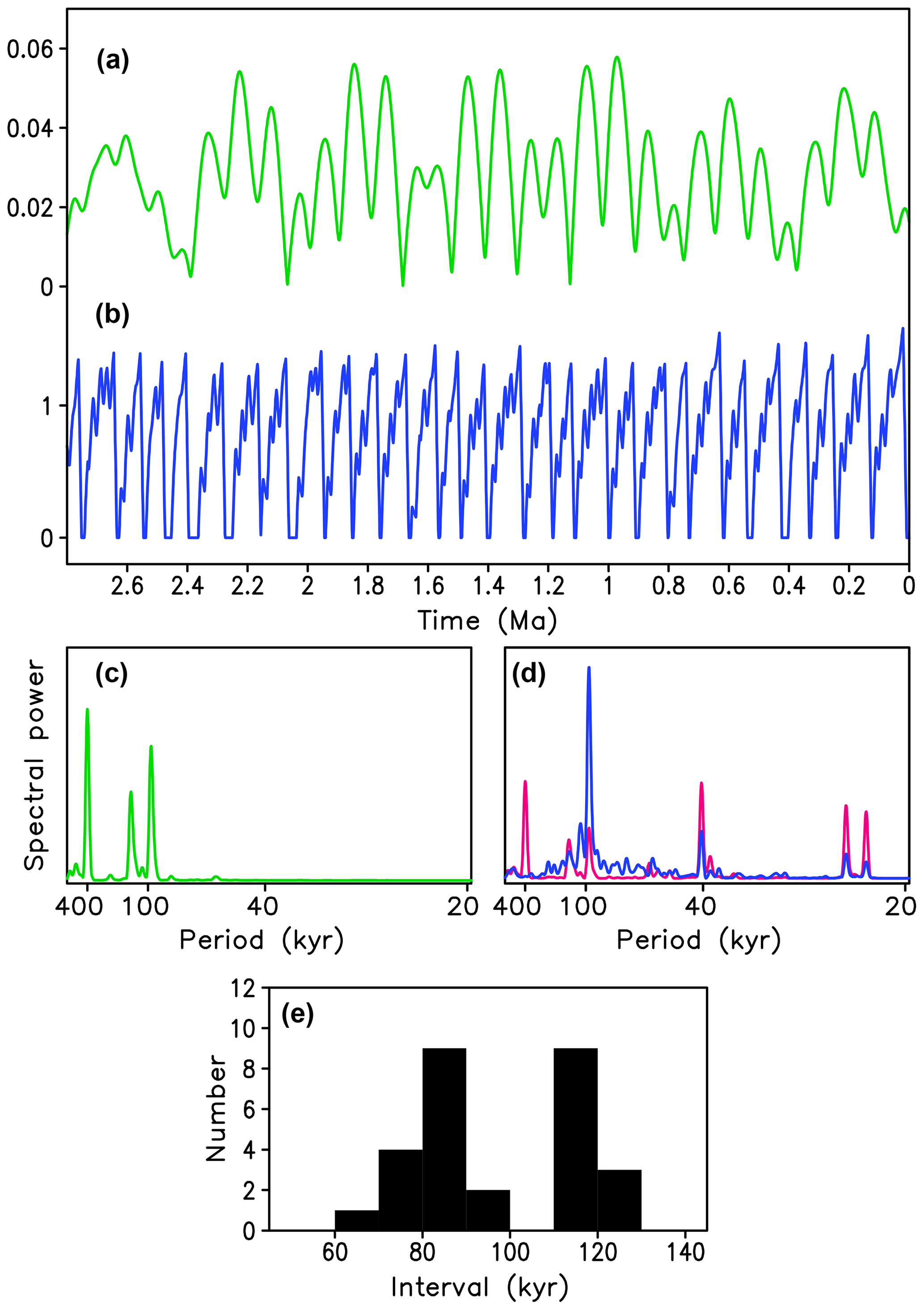
Figure 8Simulation of the last 2.8 Myr with Model 3 (vc=1.3). (a) Eccentricity, (b) simulated ice volume (arbitrary units), (c) frequency spectrum of eccentricity, (d) spectrum of ice volume simulated with Model 3 (blue) and the Imbrie and Imbrie model (magenta), (e) histogram of the durations of individual glacial cycles simulated with Model 3.
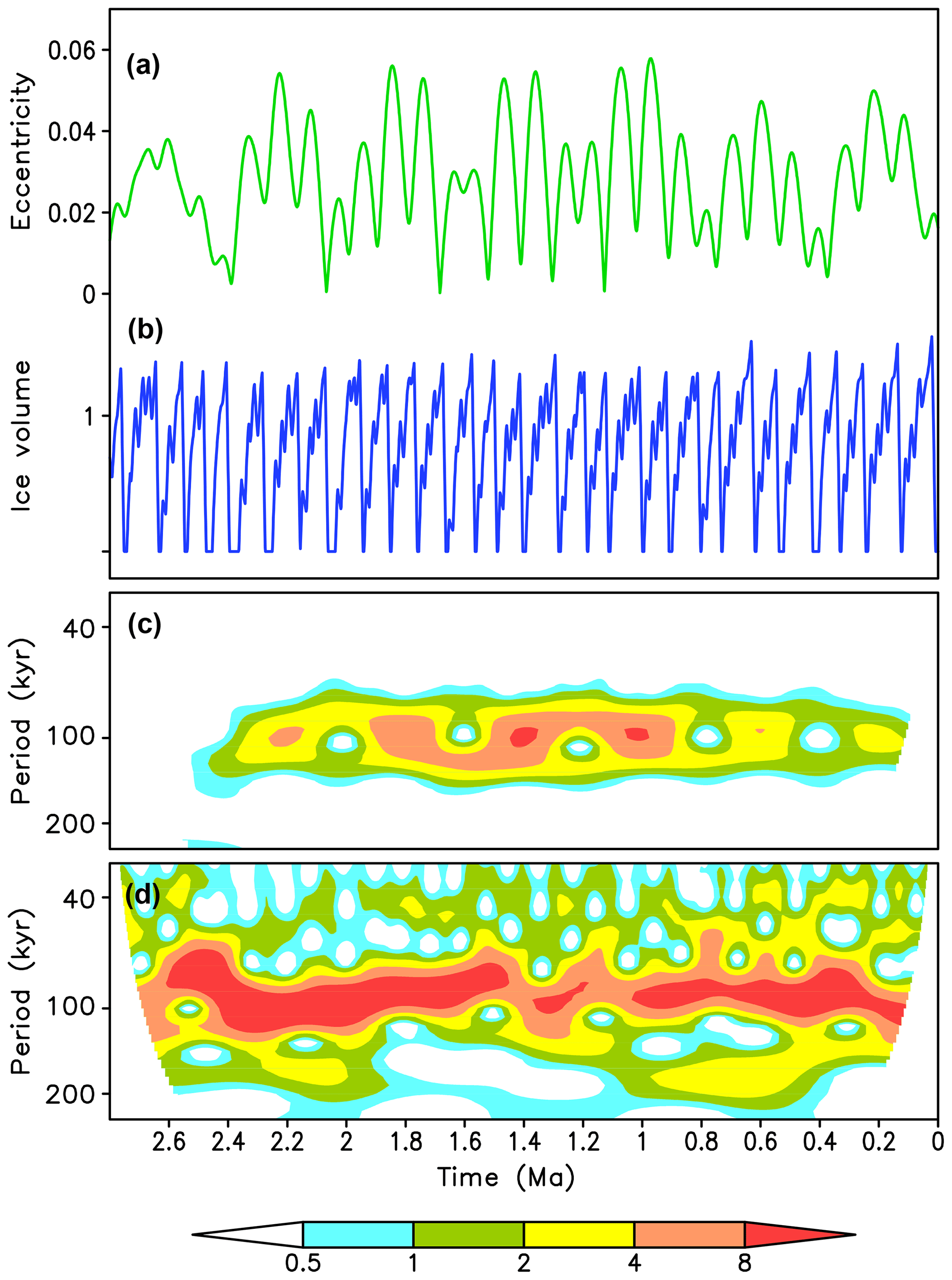
Figure 9Simulation of the last 2800 kyr with constant critical ice volume parameters (vc=1.3). (a) Eccentricity, (b) simulated ice volume (arbitrary units), (c) wavelet spectra of eccentricity, and (d) wavelet spectra of simulated ice volume.
Although the spectrum of simulated glacial cycles is dominated by a sharp peak at around 100 kyr, this does not imply that all glacial cycles have a duration close to 100 kyr. In fact, as Fig. 8e shows, the duration of individual glacial cycles tends to cluster in the intervals of 80–90 and 110–120 kyr, which are both close to the duration of two or three obliquity cycles and four or five precession cycles. On the other hand, most durations are between 80 and 120 kyr, and very few are outside, which would not be the case if glacial cycles simply lasted two or three obliquity cycles. This feature is also seen in the distribution of durations of the last eight real glacial cycles. Also, as in reality, very few simulated glacial cycles have durations between 90 and 110 kyr. This explains the apparent paradox of why none of the glacial cycles of the 100 kyr world have a duration close to 100 kyr.
Another apparent paradox related to the role of eccentricity in glacial cycles is the fact that the energy in the 100 kyr band of the ice volume spectrum was growing over the past million years while the energy in the 100 kyr band of eccentricity was decreasing during the same time (Lisiecki, 2010; see also Fig. 9). Partly, this discrepancy can be explained by the fact that the energy increase in the 100 kyr band of ice volume spectra during the mid-Pleistocene transition (MPT, ca. 1.2–0.8 Ma) was related to changes in the boundary conditions (Willeit et al., 2019). However, even when keeping model parameters constant (Fig. 9), the energy in the 100 kyr band of ice volume spectrum changes in antiphase with the energy in the eccentricity spectrum. This can again be explained by the fact that eccentricity is not the direct forcing of glacial cycles, and the amplitude of glacial cycles is not directly related to the amplitude of the 100 kyr component of eccentricity, which is also clearly seen in the experiments with the generic orbital forcing (Fig. 7).
3.6 Simulation of the mid-Pleistocene transition
When applied to the entire Quaternary, Model 3 with constant parameters tuned to the last million years fails to reproduce the glacial cycles of the early Quaternary (Fig. 9). This is consistent with Willet et al. (2019), where it was shown that orbital forcing alone could not cause the regime change a million years ago. To reproduce the MPT in P98 and Legrain et al. (2023), the critical ice volume was made time-dependent with a smaller value at the beginning of the Quaternary and a larger one toward the present. A similar approach works for Model 3 too. The critical volume vc is a nonlinear function of time:
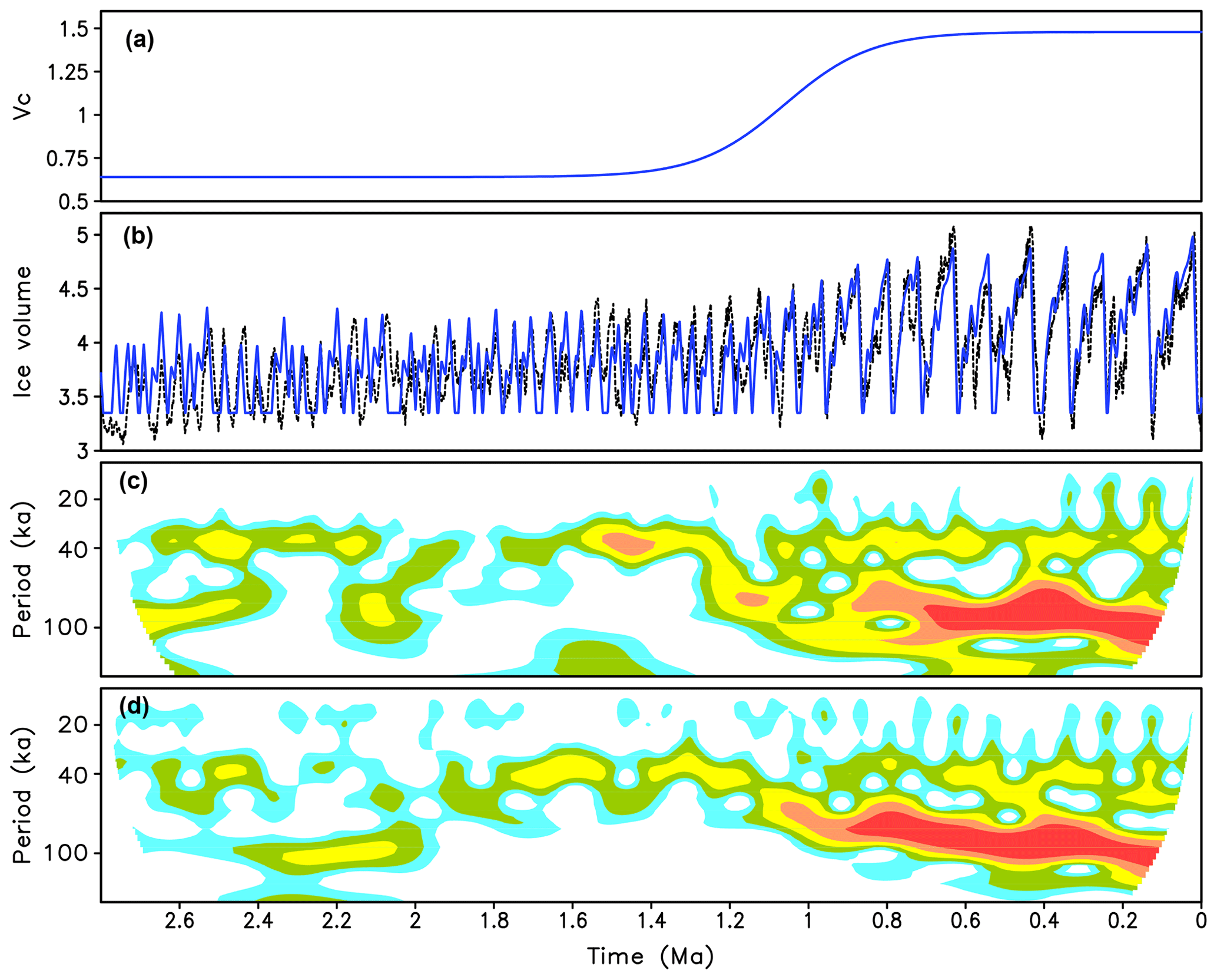
Figure 10Simulations of MPT with Model 3. (a) Temporal dependence of critical ice volume vc; (b) simulated ice volume (blue) versus LR04 (dashed); (c) wavelet spectra of LR04 stack; (d) wavelet spectra of modeled ice volume.
where t is time in kiloyears before present (negative), kyr is the center of the MPT, transition time τt=250 kyr, and the initial and final critical ice volume values are vc1=0.65 and vc2=1.38. Notably, this temporal evolution of vc closely resembles the temporal evolution of the regolith-free area prescribed in Willeit et al. (2019). Such similarity is in line with the idea that the temporal evolution of the critical size of ice sheets is controlled by sediment removal from northern continents by glacial erosion processes.
With such time-dependent vc, the model can reproduce a significant increase in the amplitude of glacial cycles and the transition from obliquity dominated 41 to 100 kyr dominated cycles around 1 million years ago. The agreement between model results and LR04 before 2 Ma is rather poor but it improves significantly after 2 Ma (Fig. 10b), and the correlation between modeled ice volume and δ18O over the last 2.7 Myr is 0.75. The wavelet spectrum of ice volume also shows good agreement with the spectrum of the LR04 stack (Fig. 10c and d). Prior to the MPT, the spectrum of modeled ice volume is dominated by obliquity even though the orbital forcing is dominated by precession. Still, the precession component is significantly stronger in model output compared to LR04. This issue will be discussed in the next section and Appendix A6. Similar to LR04 and CLIMBER-2 results (Willeit et al., 2019), the maximum energy in the wavelet spectrum in Model 3 first moves from 40 to 80 kyr (two obliquity cycles) at ca. 1.2 Ma, and only after 0.8 Ma does the 100 kyr periodicity become the dominant one. Also, in agreement with paleodata, the period of energy maximum during the last 0.8 Myr does not remain constant and shows a clear tendency to oscillate around 100 kyr with a 400 kyr periodicity, which is another eccentricity period.
3.7 Glacial cycles in Model 3
Model 3 is an example of a rather simple nonlinear transformation of the traditional orbital forcing into glacial cycles. An important feature of this model is that it is based on simulation results using the Earth system model of intermediate complexity CLIMBER-2. The key element of the model is the existence of two fundamentally different regimes: glacial with the relaxation towards one of two equilibrium states and the deglaciation regimes. The model does not possess self-sustained oscillations and has no intrinsic timescale close to 100 kyr. In fact, this period originates solely from the phase locking of long glacial cycles to the amplitude modulation of precession components of insolation by eccentricity. The model accurately reproduces not only the temporal evolution of the glacial cycles, including the timing of terminations, but also the frequency and wavelet spectra of the late Quaternary. The model helps us to understand how a dominant 100 kyr periodicity originates from the combinations of different eccentricity, obliquity, and precession periods. In the next section, I will discuss how such a mathematical transformation can be explained from the “physical” point of view.
This section presents the key elements of the GMT; namely, it discusses physical and biogeochemical processes which play a crucial role in Quaternary glacial cycles. It also explains the postulates which make Model 3 so successful. Unlike the simplicity of the conceptual model, the physical basis of the GMT is very complex, and some important processes and mechanisms are still not fully understood. This is why some aspects of the GMT are only preliminary.
4.1 Orbital forcing
When developing his theory, Milankovitch adopted the already proposed idea that changes in boreal summer insolation are critical for understanding ice ages. As the metric for summer insolation, Milankovitch used the integral of insolation during a warm (caloric) half-year. After the revival of interest in the Milankovitch theory in the 1970s, it became more common to use the maximum (or summer solstice), June, or July insolation at 65∘ N to analyze the relationship between orbital forcing and climate system response. When discussing which single metric best represents orbital forcing, it is important to realize that climate models calculate insolation at each time step and for each grid cell, and therefore climate modelers do not need to decide what definition of “summer insolation” is correct. However, for analysis of paleoclimate records and construction of simple (conceptual) models of glacial cycles, it is required to convert 3-D (latitude – day of the year – the year before or after present) insolation into a single metric. This paper uses maximum summer insolation at 65∘ N for this purpose, and this choice is discussed in Appendix A1.
Irrespective of the specific choice of the metric for orbital forcing, any summer insolation curve represents a sum of precession and obliquity components. The precession component is a quasiperiodic (T≈23 000 years) sine-like function with an amplitude proportional to eccentricity. The obliquity component is a periodic (T≈41 000 years) function with the amplitude gradually changing in time. The relative contributions of precession and obliquity components depend on the choice of latitude and definition of “summer”, but, as shown in Appendix A1, it is reasonable to assume that obliquity and precession components are of comparable importance. The only notable exception is the so-called “summer energy” proposed in Huybers (2006), containing very little precession. However, as shown in Appendix A1, “integrated summer energy” is not applicable to the problem of glacial cycles.
4.2 Climate feedbacks
Experiments with climate models which began in the 1970s confirmed the central premise of the Milankovitch theory, namely that variations of Earth's orbital parameters cause significant (several degrees and more) regional summer temperature changes over the continents. Such temperature changes would result in large vertical displacements of the equilibrium snow line and can, in principle, cause widespread glaciation of some regions. However, it has been found that the direct impact of the orbital forcing on climate in terms of global mean temperature is very small (less than 1 ∘C). Thus, to understand how orbital forcing during the Quaternary cased global-scale large-amplitude climate oscillations, it is necessary to invoke several climate-related feedbacks.
The first important positive feedback is the albedo feedback, which is already accounted for in Milankovitch calculations (Milankovitch, 1941). Results of modeling studies demonstrated that, even under a constant but sufficiently low CO2 concentration (lower than the typical interglacial level of 280 ppm), orbital forcing alone could drive glacial cycles with realistic amplitude and periodicities (Berger and Loutre, 2010; Ganopolski and Calov, 2011; Abe-Ouchi et al., 2013). In turn, large continental ice sheets strongly affect global temperature. According to model simulations, ice sheets and associated sea level drop explain about half of the global cooling at the LGM (Hargreaves et al., 2007). However, this effect caused by albedo and elevation changes over large continental ice sheets is rather local and diminishes rapidly with distance from the margins of ice sheets. Moreover, in some regions, due to the modifications of atmospheric circulation, the effect of ice sheets on temperature can even be opposite; i.e., the growth of ice sheets can cause regional warming (Liakka and Lofverstrom, 2018). Another positive feedback is related to the fact that total accumulation over the ice sheet is nearly proportional to the ice sheet area (e.g., Ganopolski et al., 2010). This feedback, although critically important for the growth of ice sheets, lacks a specific name, likely due to its apparent nature. For consistency, it can be named the area–accumulation feedback. At the same time, the expansion of Northern Hemisphere ice sheets into lower latitudes leads to an increase in ablation, and thus this area–ablation feedback is negative.
The main “globalizer” of glacial cycles is CO2, while methane and N2O together contribute about of CO2 to the radiative forcing of glacial cycles. Interestingly, the role of CO2 in glacial cycles was proposed by Svante Arrhenius (Arrhenius, 1896) well before Milankovitch published his first paper. Although Milankovitch was not enthusiastic about Arrhenius's theory, it is generally accepted now that both the Milankovitch astronomical theory and the Arrhenius CO2 theory represent two crucial ingredients of the theory of glacial cycles. The role and operation of the global carbon cycle during glacial cycles will be discussed below.
Another potentially important positive feedback (a set of feedbacks) is related to the global dust cycle. Paleoclimate reconstructions and modeling results show that the atmosphere was much dustier (typically by a factor of 2 globally) during the ice ages (Kohfeld and Harrison, 2001; Albani et al., 2018). This fact is attributed to reduced vegetation cover, exposed continental shelf, and dust production due to glacial erosion processes (Mahowald et al., 2006). Radiative forcing of aeolian dust strongly varies regionally, and its globally average magnitude remains uncertain (Bauer and Ganopolski, 2014). Apart from changing optical properties of the atmosphere, dust deposition strongly affects the surface albedo of snow and, therefore, the surface mass balance of ice sheets (Krinner et al., 2006; Ganopolski et al., 2010; Willeit and Ganopolski, 2018). In addition, a significant increase in aeolian dust deposition over the Southern Ocean through the iron fertilization effect led to an increase in net primary production of marine ecosystems and thus contributed to the glacial lowering of the atmospheric CO2 concentration (Martin, 1990; Watson et al., 2000).
Another regional feedback is climate–vegetation feedback. Modeling results suggest that the biophysical effect of vegetation cover change during glacial times produced about 0.5–1 ∘C of additional global cooling (Ganopolski, 2003; Crucifix and Hewitt, 2005; O'ishi and Abe-Ouchi, 2013) and that this feedback amplified initial cooling caused by orbital forcing over the northern continents during glacial inceptions (e.g., de Noblet et al., 1996; Calov et al., 2005b; Claussen et al., 2006). At the same time, the effect of terrestrial biosphere changes on the atmospheric CO2 concentration due to the shrinking of the terrestrial carbon pool during glacial times likely worked in the opposite direction, i.e., produced a negative feedback (see discussion below).
4.3 Timescales of the Earth system response and the nature of 100 kyr cyclicity
As shown in the previous section, the dominant periodicity close to 100 kyr of the glacial cycles during the last million years originates in our models from the phase locking of glacial cycles to the corresponding eccentricity cycle. This mechanism requires the typical duration of glacial cycles forced by obliquity and precession components of orbital forcing to be an order of 100 kyr. However, conceptual models derived from CLIMBER-2 do not have such a long internal timescale. The response time of Northern Hemisphere ice sheets to orbital forcing (30 kyr) used in Model 3 and adopted from Calov and Ganopolski (2005) is much shorter than 100 kyr. However, as shown above (see also Fig. 7), such long glacial cycles can arise if the time needed to reach a critical ice sheet volume is much larger than one precession cycle.
Admittedly, even the existence of a 30 kyr timescale of the cryosphere response to orbital forcing is not trivial. A typical accumulation rate over the Northern Hemisphere ice sheets during glacial conditions is about 0.1–0.3 Sv1 (Ganopolski et al., 2010), which is consistent with the results of LGM simulations with GCMs. The total Northern Hemisphere surface ablation and the solid ice discharge into the ocean (calving flux) vary strongly in time but are generally around 0.1 Sv each (Ganopolski et al., 2010). Thus, it would be natural to consider 0.1 Sv a typical value for the total ice sheet mass disbalance. Such an estimate corresponds to complete growth and melt of the late Quaternary ice sheet in 10 000 years, which is just one-half of the precession cycle. In reality, such a rate of change is only achieved during glacial terminations, while for the rest of glacial cycles, the typical rate of global ice volume change was several times smaller, which implies that the positive and negative components of the ice sheet mass balance are close to each other by absolute values most of the time. This can be explained by the fact that, apart from the positive albedo and elevation feedbacks, there is strong negative feedback associated with ice sheet southward expansion. Model simulations show that the positive component of mass balance (accumulation) is roughly proportional to the size of ice sheets, whereas ablation increases strongly nonlinearly with the southward expansion of ice sheet margins. This negative feedback prevents North American and Eurasian ice sheets from spreading into low latitudes. As a result, reaching the equilibrium state takes much longer than one would expect from a simple scale analysis. Only under extremely strong orbital forcing (during periods of high eccentricity) can the disbalance between the components of surface mass balance be much larger, and the rate of volume changes increases substantially. This can explain a few “short” glacial cycles at ca. 600 and 220 ka, which Model 3 cannot simulate by design.
As shown in experiments with Model 3, phase locking of glacial cycles to the 100 kyr periodicity of eccentricity originates from the highest likelihood of reaching the critical ice volume during periods of low eccentricity. This is explained by the fact that, while high eccentricity facilitates ice sheet growth during glacial inceptions, the critical ice volume can be reached only if the system stays sufficiently long in the attraction domain of the glacial state, which occurs during periods of low eccentricity. In the case of realistic orbital forcing, the largest probability of reaching the critical ice volume is when a relatively weak maximum of the precession component of insolation coincides with a minimum of obliquity. Thus, according to GMT, the timing and periodicity of glacial cycles of the late Quaternary are set by the shortest (100 kyr) eccentricity cycles. The appearance of the eccentricity period in the spectra of glacial cycles originates from the phase locking rather than the forcing of glacial cycles by eccentricity. This concept eliminates the main criticism of “the eccentricity myth” (Maslin and Brierley, 2015) based on the fact that the direct impact of eccentricity on insolation in terms of the global mean value is too small (about 0.5 W m−2) to affect glacial cycles. According to GMT, eccentricity affects glacial cycles indirectly through its amplitude modulation of the precession component of insolation, which results in the variations of maximum boreal summer insolation at the top of the atmosphere with an amplitude of more than 50 W m−2.
Obliquity plays a role in setting the timing of glacial cycles, but as was shown in Ganopolski and Calov (2011), the dominant 100 kyr cyclicity is simulated by CLIMBER-2 even if the obliquity component is artificially eliminated from orbital forcing. The main difference in simulations with and without the obliquity component (see Fig. 3d in Ganopolski and Calov, 2010) is that the elimination of obliquity leads to an increase in energy in the 405 kyr band, which is another eccentricity period. A qualitatively similar effect is seen in Model 3 results (Appendix A5, Fig. A6), but the magnitude of the 405 kyr peak is strongly parameter-dependent. Thus, although obliquity affects the duration of individual glacial cycles, it plays no role in setting the 100 kyr periodicity. In other words, 100 kyr periodicity originates not from the fact that glacial cycles tend to last two or three obliquity cycles with equal probability as proposed by Huybers and Wunsch (2005), but, to the contrary, glacial cycles typically lasted two or three obliquity cycles because kyr is the periodicity of eccentricity to which long glacial cycles of the late Quaternary are tightly phase-locked.
It is important to stress that, although a sharp peak at 100 kyr in the frequency spectra of the late Quaternary climate variability is successfully reproduced by several physically based models and is robust within a broad range of the parameters of conceptual models, this is a rather peculiar regime of operation of the Earth system. Such a regime is only possible for a “proper” combination of orbital forcing and key boundary conditions: position of continents, regolith distribution, and CO2 level, among others. This is why this regime was established only about 1 Ma, and it is likely that it will change to another regime in the future due to the natural evolution of the Earth system.
4.4 Multiple equilibrium states of the climate–cryosphere system and escape from the glacial trap
As shown in the previous section, the conceptual model based on multiple equilibrium states successfully simulates Quaternary glacial cycles. The idea that the climate–cryosphere has several equilibrium states has a long history (e.g., Budyko, 1972; Weertman, 1976; Benzi et al., 1982). Multiple equilibrium states of the climate–cryosphere system have also been found in several models that explicitly included ice sheet components (e.g., Pollard and DeConto, 2005; Calov and Ganopolski, 2005; Robinson et al., 2012; Abe-Ouchi et al., 2013). These studies show that different ice sheets have very different stability diagrams in the phase space of orbital forcing, temperature, or CO2. In the simplest case, the stability diagram of an ice sheet in the phase space of orbital forcing (maximum summer insolation at 65∘ N) is represented by two branches (glacial and interglacial) as in Model 3 (Fig. 11a). It is also common for illustrating purposes to depict such a bi-stable system in the form of double-well Lyapounov potential (Fig. 11b). Each well represents one of the equilibrium states, and the depth of the wells represents the stability of each state. Since the shape of such a diagram depends on orbital forcing itself, the diagram in Fig. 11b shows potential for average orbital forcing, i.e., zero forcing anomaly.
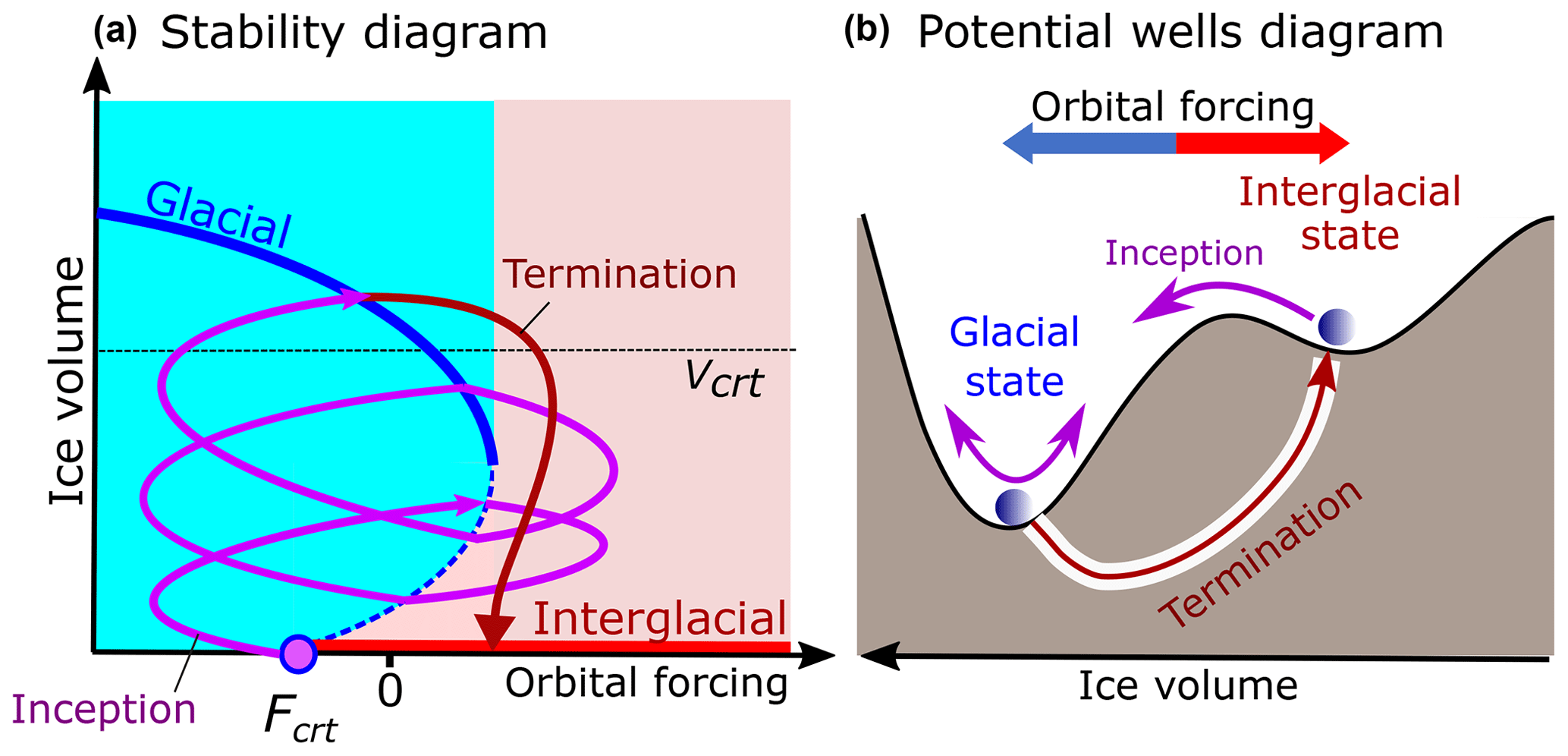
Figure 11Generalized stability diagram of the climate–cryosphere system. (a) Phase portrait in orbital forcing (anomaly of maximum summer insolation at 65∘ N) space. The notations are the same as in Fig. 4a. (b) Two potential wells represent the glacial and interglacial states. The diagram corresponds to the average (zero) orbital forcing, while orbital forcing is considered here to be the external perturbation which moves the system from one equilibrium to another one. Glacial termination is depicted as the tunnel transition under the potential barrier separating two stable states.
If the system is in the interglacial state, it will remain in this state as long as the orbital forcing stays above the critical threshold value Fcrt. This value depends on CO2 concentration (Calov and Ganopolski, 2005; Archer and Ganopolski, 2005). In Ganopolski et al. (2016), this dependence on CO2 has been systematically studied, and a simple logarithmic relationship between the critical value of insolation and CO2 concentration has been found:
where α and β are constants. In the phase space of orbital forcing, glacial inception represents a bifurcation transition from the glacial to the interglacial state (Calov et al., 2005a). However, this transition is “abrupt” only in the phase space. In reality, because of the very long response time of the climate–cryosphere system to orbital forcing, the system's trajectory differs significantly from the stability diagram shown in Fig. 11a. However, when the system enters the glacial cycle, it tends to stay longer in the domain of the attraction of glacial equilibria even though insolation is below its critical value Fcrt on average significantly less than 50 % of the time. Figure 11a illustrates this “irreversibility” of glacial inception. While such behavior is entirely consistent with the paleoclimate reconstructions, the principal question arises: if the glacial equilibrium is so stable, why does the Earth system rapidly move into the interglacial state instead of oscillating around the glacial equilibrium state? In other words, how does the Earth system escape its glacial trap? The stability diagram alone shown in Fig. 11a cannot explain such behavior because, as shown above, based on this stability diagram, Model 3 cannot simulate deglaciation without introducing an additional deglaciation regime shown in Fig. 11a by the red line. In Fig. 11b this deglaciation trajectory is shown as the transition through the potential barrier separating two wells. To some extent, this process is analogous to the quantum tunnel effect. This mechanism of escape from the glacial trap represents one of the key elements of the GMT and is discussed below.
4.5 Glacial terminations: the domino effect
The most serious challenge to the classical Milankovitch theory is the strong asymmetry of the glacial cycles during the late Quaternary. The domination of such long glacial cycles requires a relatively small ice sheet to survive periods of rather high summer insolation while larger ice sheets vanish completely even after modest insolation rise as happened, for example, at the onset of MIS 11 ca. 430 ka. The instability of the ice sheets after reaching a “critical size” has been postulated in P98 and is also essential for conceptual models described in this paper. The question is how to explain this instability and what critical size means. The analogy with the mechanical “domino effect” is helpful in answering these questions.
The domino is an example of a mechanical system with different equilibrium states and can respond to an external forcing both linearly and strongly nonlinearly (the domino effect) depending on one parameter value – the distance between the dominos. Let us consider a pendulum hitting the row of dominos, as shown in Fig. 12. If this distance between dominoes is even slightly larger than the height of dominoes, the pendulum will only knock down the dominoes within its reach. In this case, the number of dominoes that fall is proportional to the amplitude of pendulum oscillations. However, if the distance between dominoes is only slightly smaller than their height (this is the situation used in demonstrations of the domino effect), then all dominoes in the row will fall irrespective of the amplitude of pendulum oscillations.
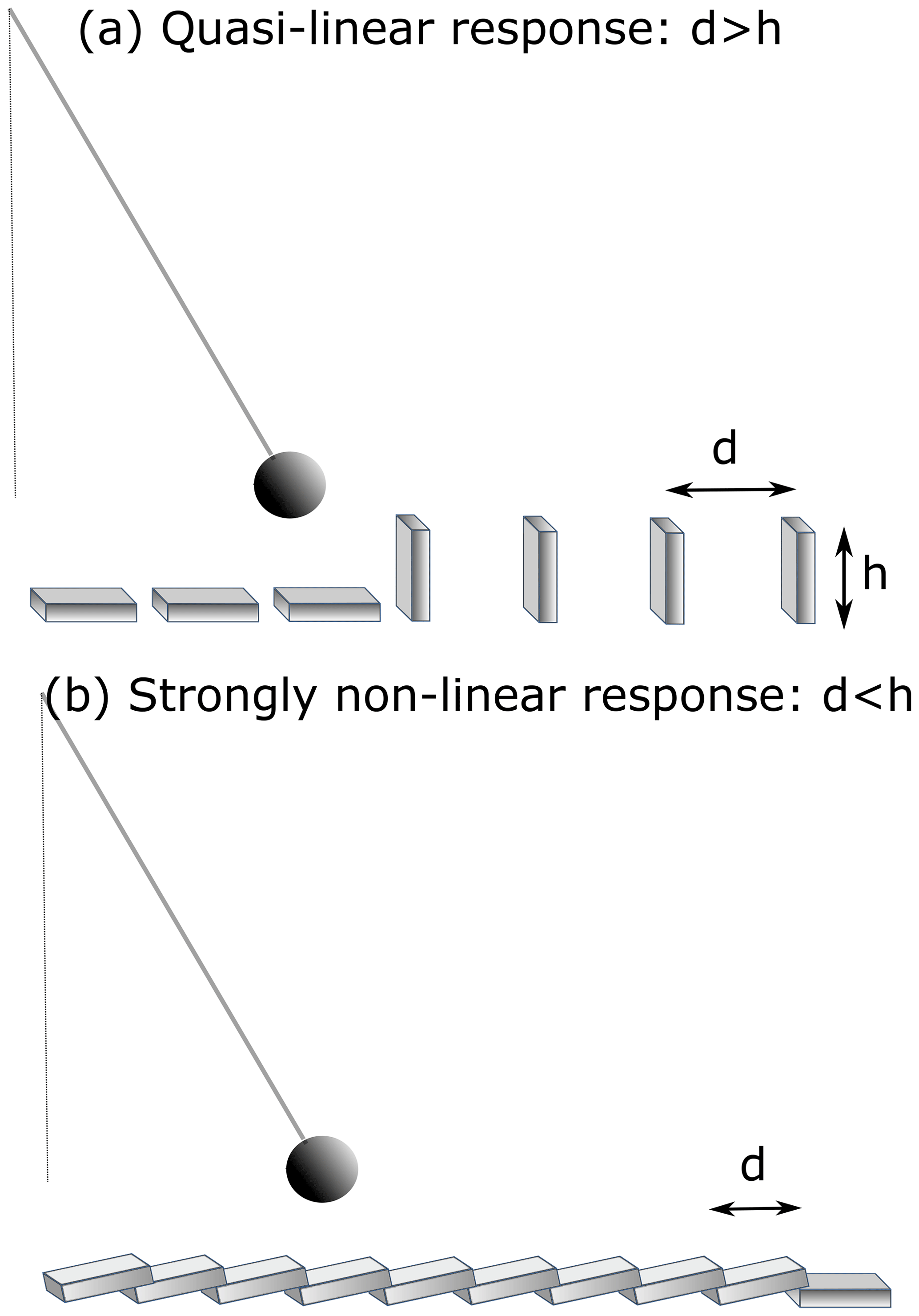
The unstoppable retreat of the Northern Hemisphere ice sheets, which occurs in response to insolation rise and the final result of which (complete deglaciation) does not depend on the magnitude of insolation rise, resembles the domino effect. In this case, the analog for the distance between the dominoes is the critical size of ice sheets. Analysis of CLIMBER-2 model simulations suggests that the concept of critical size applies primarily to the North American ice sheet since the response of the smaller Eurasian ice sheet to orbital forcing is more linear. Other opinions exist; for example, Paillard and Parrenin (2004) attributed critical size to the Antarctic ice sheet.
What causes the domino effect in the case of supercritical ice sheets? It is likely that at least several processes and mechanisms must be considered to explain why a large North American ice sheet is so sensitive to insolation rise and can vanish at a timescale about or even shorter than 10 000 years.
-
A large North American ice sheet spreads over the vast areas covered by unconsolidated sediments (Great Lakes region, the western prairies of the US and Canada), where the ice sheet is thinner and flatter than over areas with exposed rocks. This is explained by a much larger basal sliding velocity over unconsolidated water-saturated sediments than bare rocks (e.g., Licciardy et al., 1998). This implies that the slope of a large ice sheet near its margins is less steep, and as a result, the ablation area is larger (Fig. 13a), which explains the higher sensitivity of the surface mass balance of such ice sheet to insolation and CO2 rise.
-
The expansion of ice sheets over the areas covered by a thick terrestrial sediment layer leads to the production of a large amount of glaciogenic dust, which originates from the sediments transported beneath ice sheets across their margins (Mahowald et al., 2006; Ganopolski et al., 2010). A fraction of these sediments become airborne, and while this glaciogenic dust precipitates over the ice sheet, it significantly reduces surface reflectivity as the albedo of snow is very sensitive to even a tiny concentration of impurities. (Warren and Wiscombe, 1980; Dang et al., 2015). This, in turn, has a significant impact on the surface mass balance of ice sheets (Krinner et al., 2006; Willeit and Ganopolski, 2018) and causes the ice sheets to retreat earlier (Fig. 13b).
-
The weight of a mature ice sheet causes significant bedrock depression, roughly equal to of the ice sheet thickness, i.e., reaches more than 1 km in the center of continental ice sheets. A typical timescale of the bedrock relaxation towards its unperturbed (approximately modern) state after the removal of the ice sheet is about 5000 years, which is small compared to the timescale of a glacial cycle (100 kyr) but is comparable to the timescale of glacial terminations (10 kyr).
In the case of rapid retreat of ice sheets, delayed bedrock rebound facilitates surface melt. This is explained by the fact that, for the same thickness of ice sheet, the surface elevation in the ablation zone is lower in the case of delayed relaxation than it would be in the case of instantaneous bedrock adjustment (Fig. 13c). The role of delayed bedrock adjustment in the shaping of glacial cycles has already been demonstrated in Oerlemans (1980) and Pollard (1983). Simulations with a 3-D ice sheet model (Abe-Ouchi et al., 2013) confirmed that delayed bedrock adjustment is important for the complete deglaciations of the Northern Hemisphere at the end of each glacial cycle.
-
Another mechanism which can contribute to fast deglaciation is the so-called “marine ice sheet instability” (Weertman, 1974). This mechanism requires the base of the ice sheet to be located below sea level and the retrograde slope of bedrock (the elevation of bedrock decreases inland). This mechanism can cause a relatively rapid (millennial timescale) disintegration of a significant fraction of the ice sheet without significant surface mass loss. It was proposed that the Barents ice sheet disintegrated through this mechanism around the Bølling warm event (Brendryen et al., 2020).
-
The idea that the formation of proglacial lakes south of the ice sheets during their final retreat plays an important role during glacial terminations (Andrews, 1973) was also first tested in Pollard (1983). Large proglacial lakes are formed in depressions resulting from delayed bedrock relaxation in the process of fast ice sheet retreat. These depression areas are filled by the water from melting ice sheets, and their level can be well above sea level. The formation of the proglacial lakes leads to another mechanism of ice sheet instability which can be considered the freshwater analog of marine ice shelf instability (Quiquet et al., 2021; Hinck et al., 2022). The appearance of proglacial lakes causes a significant increase in the ice flux through the grounding line into the lakes (Fig. 13d). This ice then rapidly melts because it has a low elevation.
-
Rapid CO2 rise during glacial terminations plays a role in tandem with the insolation rise during glacial terminations. The modeling study suggests that both factors play a comparable role in the ice sheet mass loss (Heinemann et al., 2014; Gregorie et al., 2015). The rapid melting of ice sheets during terminations results in large freshwater flux into the North Atlantic (0.1–0.2 Sv) sufficient to cause a prolonged shutdown of the AMOC, which in turn additionally contributes to the deglacial CO2 rise and its overshoot at the end of deglaciation (Ganopolski and Brovkin, 2017). At the same time, AMOC shutdown during deglaciation causes anomalous cooling over Europe and slows down deglaciation (negative feedback). Additionally, subsurface warming induced by the AMOC shutdown can destabilize ice shelves in the North Atlantic realm (see below). The net effect of AMOC changes on deglaciation still has to be evaluated with adequate Earth system models.
All mechanisms discussed above are likely important for the domino effect. Each of the mechanisms discussed above should not necessarily be “catastrophic”, but when they work together, the combined effect can cause rapid disintegration of large continental ice sheets. It is also important to stress that none of these mechanisms are specific for the 100 kyr world – all of them also operated during the 41 kyr world and MPT. According to GMT, the difference between the 41 kyr world and 100 kyr world is in the critical size of ice sheets after exceedance of which the mechanisms discussed above lead to rapid deglaciation of the Northern Hemisphere.
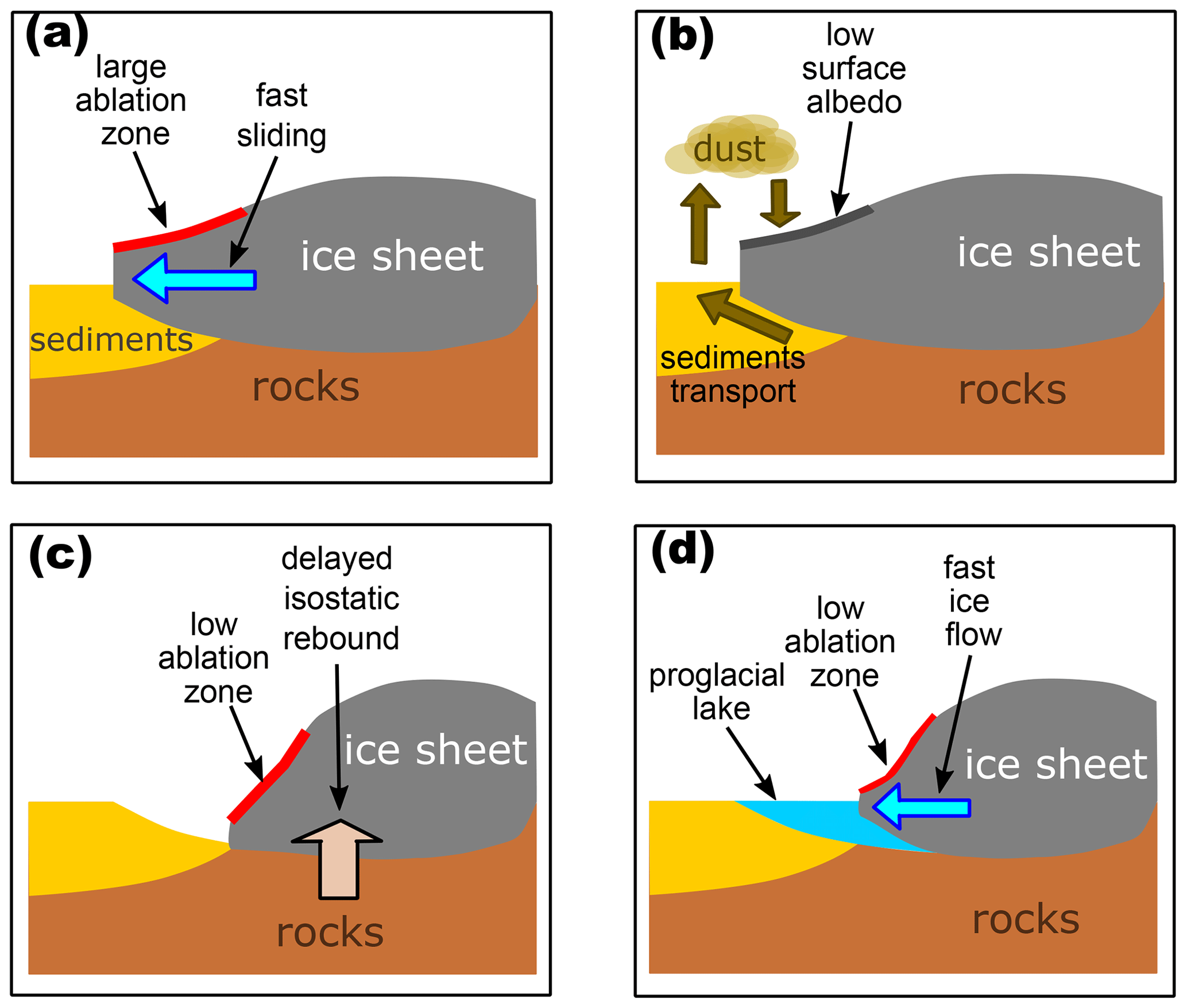
Figure 13The principal elements of the termination mechanism: (a) faster ice sliding and lower elevation over sediment area; (b) effect of glaciogenic dust deposition on snow albedo and surface mass balance; (c) effect of delayed bedrock relaxation on the altitude of ablation zone; (d) effect of proglacial lakes on ice sheet mass loss.
4.6 The role of climate–carbon cycle feedbacks
It is generally recognized that CO2 plays a vital role in the dynamics of glacial cycles. It is also important to distinguish between the “effect” of glacial CO2 on climate variability and the role of carbon cycle feedback during glacial cycles. On geological timescales, the average CO2 concentration is controlled by the interplay between volcanic outgassing and weathering rate. In turn, this concentration controls the amplitude of glacial cycles (Berger et al., 1999; Ganopolski and Calov, 2011; Abe-Ouchi et al., 2013), and for a sufficiently high CO2 concentration, glacial cycles are not possible for a realistic range of the Earth's orbital parameters. This is why gradual lowering of the CO2 concentration below a certain threshold was one of the preconditions for the onset of Quaternary glacial cycles (Willeit et al., 2015). After the CO2 concentration dropped below this threshold and regular glacial cycles began, climate–carbon cycle feedback amplified glacial cycles, especially their 100 kyr component, and also globalized their impact on climate.
The quest for the mechanisms of glacial–interglacial CO2 variability discovered thanks to the Antarctic ice cores (Petit et al., 1999; Lüthi et al., 2008) has attracted significant attention during the past 2 decades. However, the mechanisms of this variability are still not fully understood. Results of numerous modeling studies strongly indicate that there is no single mechanism that can explain most of the observed glacial–interglacial CO2 changes of about 100 ppm, and it has become increasingly clear that at least several processes should be involved (e.g., Archer et al., 2000; Kohfeld and Ridgwell, 2009). Moreover, it is likely that the roles of geochemical (inorganic) and biogeochemical processes in glacial–interglacial CO2 variability are of comparable importance (Galbraith and de Lavergne, 2019). It is much more certain that glacial CO2 lowering can only be explained by the ocean carbon uptake since the terrestrial carbon pool was significantly depleted during glacial times due to the shrinking of the vegetation cover (Brovkin et al., 2012; Jeltsch-Thommes et al., 2019). It should be noted that, apart from the redistribution of carbon between atmospheric, land, and ocean pools, the disbalance between volcanic outgassing and weathering rate may also play a role in CO2 variability at orbital and longer timescales.
It is known that the CO2 concentration and global ice volume during the late Quaternary are highly correlated – the correlation coefficient between CO2 and ice volume is above 0.7 for the last 800 kyr. However, the high correlation alone says nothing about causal relationships. Modeling studies suggest that the direct response of the carbon cycle to orbital forcing is weak. This is also supported by the fact that obliquity and precession components are relatively weak in CO2 records of the late Quaternary. At the same time, modeling results demonstrate that strongly asymmetric glacial cycles with the dominant 100 kyr periodicity can be simulated even with a constant CO2 concentration if this concentration is sufficiently low (Ganopolski and Calov, 2011; Abe-Ouchi et al., 2013). This is consistent with the concept that 100 kyr cyclicity originates from a nonlinear response of the climate–cryosphere system to orbital forcing and that the climate–carbon cycle feedback amplifies the 100 kyr component of glacial cycles (Ganopolski and Brovkin, 2017). However, while the influence of CO2 through climate on global ice volume is rather straightforward, the influence of ice sheets on CO2 concentration is far from trivial. The most direct effect of ice sheet growth on CO2 is through the decrease in the ocean volume, which leads to the effect opposite to the observed CO2 changes. Indeed, the decrease of the ocean volume by ca. 3 % at the LGM would cause CO2 to rise by about 10 ppm. In addition, the growth of ice sheets reduces forest area in the boreal zone, which should also cause a CO2 rise. The direct effect of ice sheets on the carbon cycle, which can contribute to the glacial CO2 drawdown, is regional cooling due to higher albedo of ice sheets. This cooling leads to a lowering of ocean temperature, mainly in the vicinity of the ice sheets, and contributes to CO2 decrease through the solubility effect. However, changes in ice sheet area primarily affect the climate of the Northern Hemisphere, and even the total solubility effect (including lowering of CO2 and other GHG concentrations) explains not more than 30 ppm of glacial CO2 decrease (Brovkin et al., 2007; Kohfeld and Ridgwell, 2009).
In addition to global ocean volume change, ice sheets can affect CO2 through global sea level change. First, this leads to a change in ocean alkalinity through the dissolution or regrowth of shallow-water carbonates, particularly in the form of corrals (Ridgwell et al., 2003). Higher alkalinity, which results from the sea level drop, increases ocean capability to absorb atmospheric CO2 and thus contributes to glacial CO2 drawdown. Second, exposed shelves may represent significant additional sources of aeolian dust, and enhanced dust deposition can intensify marine biological productivity in the Southern Ocean, which is iron-limited (Martin, 1990; Watson et al., 2000; Yamamoto et al., 2019). Third, due to the peculiar oceanic hypsometry, even a relatively small initial sea level drop leads to a significant increase in land area. This not only contributes to additional global cooling but also leads to an expansion of vegetation cover and thus serves as the carbon uptake. The latter can work only during the initial phase of glacial cycles because, under full glacial conditions, global decline in terrestrial biomass due to ice sheet expansion and CO2 lowering overwhelms the effect of land area increase. In this way, there are at least several mechanisms through which ice sheets can cause changes in CO2 coeval with ice volume changes.
This initial response of atmospheric CO2 to ice sheet evolution is amplified by several climate–carbon cycle feedbacks: (1) enhanced ocean carbon uptake due to cooling, i.e., solubility effect, in addition to the effect caused by ice sheet growth; (2) the effect on ocean carbon storage caused by changes in the ocean circulation, stratification, and sea ice cover, leading to changes (reduction) in the deep ocean ventilation; and (3) a change in the remineralization depth caused by ocean thermocline temperature lowering, which affects organic carbon flux into the deep ocean. Although the operation of the global carbon cycle during glacial times is still not fully understood, it is likely that the direct effect of ice sheets on CO2 and the effect of its amplification via climate–carbon cycle feedbacks are of comparable importance.
4.7 Glacial cycles of the early Quaternary (41 kyr world)
Prior to the MPT (ca. 1.2–0.8 Ma), glacial cycles had a smaller magnitude (50 % when compared to the late Quaternary in terms of benthic δ18O), and the dominant periodicity was 41 kyr, which is the periodicity of obliquity with very little energy in the 100 kyr and precession bands (Fig. 2). According to the GMT, a shorter periodicity and smaller magnitude of early Quaternary glacial cycles are explained by the fact that the critical size of ice sheets, which makes the Earth system prone to deglaciation, was smaller before the MPT than after. The most likely explanation for that (see also the next section) is the gradual removal of terrestrial sediments from North America by glacial erosion (Clark and Pollard, 1998). The thick terrestrial sediments make ice sheets more mobile since “temperate” ice (ice at the pressure melting point) moves much faster over sediments than over bare rocks. Thus, the presence of thick sediments allows ice sheets to spread faster and makes them thinner, which also explains the larger sensitivity of ice sheet mass balance to orbital forcing. In addition, the spreading of ice sheets over terrestrial sediment led to the production of a large amount of glaciogenic dust, some of which was then deposited over ice sheets, making them darker and thus increasing surface ablation (Ganopolski and Calov, 2011). As a result, the early Quaternary ice sheets were able to reach their critical size during just one obliquity cycle. Since glacial cycles were much shorter, these cycles look more symmetric than the late Quaternary cycles, but this does not mean that the response of the Earth system to orbital forcing was linear, and it is likely that all elements of the domino effect also operated during glacial terminations of the early Quaternary.
While the dominance of the obliquity component in ice volume variations during the early Quaternary is not surprising and is reproduced in model simulations (Ganopolski and Calov, 2011; Willeit et al., 2019), a strong precession component is also clearly present in the spectra of simulated ice volume. At the same time the precession component is essentially absent during the early Quaternary in many paleoclimate reconstructions, including the canonical LR04 benthic stack. This mismatch is often considered another unsolved problem (“mystery”) of the Milankovitch theory (Raymo and Nisancioglu, 2003). A number of explanations for the lack of precession components prior to MPT have been proposed, including the possibility of mutual compensation of precession components originating from the evolution of southern and northern ice sheets (Raymo et al., 2006). However, in recent years, a precession signal during the early Quaternary has started to emerge in paleoclimate records (e.g., Shakun et al., 2016; Liautaud et al., 2020; Barker et al., 2022), and there may be an inherent issue with absolute dating of old paleoclimate records. Appendix A6 illustrates how a simple “orbital tuning” can nearly completely eliminate the precession signal from the ice volume record. However, there is another often overlooked aspect of the 41 kyr mystery: it is generally assumed that the entire Quaternary records are dominated by ice volume variability. While about of benthic δ18O variability (or 80 % in spectral power) is attributed to global ice volume change during the late Quaternary, results of model simulations (Willeit et al., 2019) show that the relative contribution of ice volume to benthic δ18O was only about (or only 20 % in the frequency spectra) before the MPT. This is consistent with Elderfield et al. (2012), which also found that the relative contribution of deep ocean temperature to δ18O prior to MPT was significantly higher than 50 %. This would change the 41 kyr mystery from the challenge of explaining the absence of precession component in global ice volume (which is indeed hard to explain) to the question of why the deep ocean temperature does not contain much precession variability. The latter is a different problem since the deep ocean temperature is controlled by different factors than the ice volume, primarily by CO2 concentration. Since CO2 concentration over the past 800 kyr contains very little precession variability (e.g., Petit et al., 1999), it would be natural to assume that this was also the case during the early Quaternary. Thus, the 41 kyr mystery cannot be considered a fundamental problem of the Milankovitch theory.
4.8 Three Quaternary regime changes: PPT, MPT, and MBT
During the past 3 million years, climate variability at orbital timescales revealed three distinct changes in the mode of operation. The first one, referred to as the Pliocene–Pleistocene transition (PPT), is the onset of regular glacial cycles with the dominant 41 kyr periodicity, which happened between 2.8 and 2.7 Ma, i.e., significantly earlier than the “official” stratigraphic Pliocene–Pleistocene border (2.58 Ma). The second transition, the mid-Pleistocene transition (MPT) from the 41 to 100 kyr world, occurred between 1.2 and 0.8 Ma. The third transition, clearly seen only in some paleoclimate records (such as δ18O and CO2), is referred to as the mid-Brunhes transition2 and manifests itself in the differences between interglacials before and after MIS 11.
The onset of Quaternary glacial cycles was preconditioned by the general Cenozoic cooling trend (Raymo and Ruddiman, 1992) caused by decreasing CO2 concentration and the poleward advance of North America during the Cenozoic epoch (Daradich et al., 2017). Several additional proximal causes, including the closing, opening, or deepening of different oceanic gateways and establishing of North Pacific stratification, have been proposed to explain the PPT (e.g., Ruddiman and Raymo, 1988; Cane and Molnar, 2001; Haug and Tiedemann, 1998; Haug et al., 2005) but the role of these events in the onset of Quaternary glacial cycles is not clear. At the same time, it has been shown (Willeit et al., 2015) that even a gradual downward CO2 trend alone is sufficient to cause the transition from an essentially ice-free Northern Hemisphere to glacial cycles of medium amplitude after the PPT. The critical value of CO2 concentration of 350–400 ppm, below which regular glaciations in the Northern Hemisphere can begin (Ganopolski et al., 2016), is consistent with the recent CO2 reconstructions during the PPT (Martínez-Botí et al., 2015).
In the 1.5 million years which followed the PPT, the magnitude of glacial cycles increased gradually, but the dominant periodicity (41 kyr) remained unchanged. However, between 1.2 and 0.8 Ma, climate variability recorded by δ18O changed dramatically from relatively symmetric cycles of the 41 kyr world to strongly asymmetric 100 kyr cycles. The magnitude of glacial cycles expressed in the standard deviation of benthic δ18O doubled across the MPT (Lisiecki and Raymo, 2007).
The MPT has been attributed by Clark and Pollard (1998) to a gradual evolution of terrestrial sediment cover over northern continents (the so-called “regolith hypothesis”). This hypothesis is based on the empirical fact that at present large areas of northern North America and Eurasia are characterized by a thin layer of terrestrial sediments or exposed crystalline rocks, while the rest of these continents are covered by kilometer-thick terrestrial sediments. Since the areas of thin sediments and exposed bedrock coincide with the areas covered by ice sheets most of the time during the Quaternary, it is natural to assume that, prior to the Quaternary, these areas were also covered by a thick sediment layer which was then gradually removed by glacial erosion processes. In turn, the underlying surface type (crystalline rocks or unconsolidated terrestrial sediments) strongly affects ice sheet dynamics as ice can slide much faster over sediments (compared to rocks) when the temperature at the base of ice sheets reaches the pressure melting point. This can explain why ice sheets of the early Quaternary were thinner and thus more susceptible to insolation changes. As a result, ice sheets during the early Quaternary responded to orbital forcing in a more linear manner without any appreciable contribution from the eccentricity cycles. The appearance of large areas of exposed crystalline rocks about 1 million years ago led to the formation of thick and slower-spreading ice sheets with a narrower ablation zone. The latter helped ice sheets to survive several insolation maxima before they spread deep enough into the sediment-covered areas, which made them prone to a rapid collapse during insolation rise. In Ganopolski and Calov (2011) we proposed an additional mechanism that might contribute to the MPT and which is also related to the removal of the regolith layer from the northern continents. This mechanism is based on the fact that, when ice sheets spread over the areas covered by terrestrial sediments, they produce a significant amount of glaciogenic dust, which, in turn, affects surface albedo and ablation (see Sect. 5.5). While this mechanism operated through the entire glacial cycle before the MPT as northern continents were covered by terrestrial sediments, ice sheets spread over the sediment-covered areas only after they approached their critical size after the MPT. Both these mechanisms were incorporated into the CLIMBER-2 model and contributed to the realistic simulation of MPT (Willeit et al., 2019).
It has also been shown by Willeit et al. (2019) that even a gradual expansion of the sediment-free areas from zero to the present one over the past 1500 kyr can explain a relatively rapid transition (over several hundred thousand years) from the 41 to 100 kyr regime. In other words, it has been shown that there is a critical threshold for the exposed rock area, crossing of which leads to the transition from 41 kyr cyclicity to 100 kyr cyclicity. It has to be noted that a gradual reduction of the CO2 concentration during the Quaternary is considered by some authors (e.g., Berger et al., 1999) to be a possible cause of MPT, but according to Willeit et al. (2019), it is not an alternative mechanism of MPT but rather an important precondition for the onset of long glacial cycles, since for high CO2 concentrations, only relatively weak and short glacial cycles are possible even for the present-day regolith distribution (Fig. S9 in Willeit et al., 2019). Thus, the onset of the 100 kyr world has been preconditioned both by CO2 decline and regolith removal. However, the timing of the MPT was likely set by the regolith removal since there is no strong evidence for the decline of the CO2 level directly prior to the MPT (Hönisch et al., 2009; Chalk et al., 2017; Yamamoto et al., 2022).
Apart from regolith removal and CO2 lowering, several other mechanisms have been proposed to explain the MPT. For example, it has been speculated that this regime change in glacial climate variability may have been related to changes in the operation of the global carbon cycle and ocean circulation (e.g., Chalk et al., 2017; Farmer et al., 2019; Hasenfratz et al., 2019). However, it is also possible that observed changes in any paleoclimate proxy across the MPT can result from the increase in the magnitude of glacial cycles (i.e., ice volume variations) and not be the cause of this change. It is also likely that the larger magnitude of sea level and temperature fluctuations after the MPT can also explain the expansion of the marine-based Antarctic ice sheet (Ford and Raymo, 2020; Sutter et al., 2019). Only results of Earth system model simulations can confirm or reject a possible contribution of all these mechanisms to the MPT.
The last transition – MBT – is less clearly defined, and the number of long glacial cycles before and after the MBT is too small to obtain robust statistics. The most apparent change across the MBT is seen in δ18O and CO2 during interglacials. These differences are consistent with the idea that pre-MBT glacial terminations were “incomplete” and that a certain amount of “glacial” ice (ca. 10–20 m in sea level equivalent) remained in ice sheets and/or ice caps in the Northern Hemisphere outside of Greenland during pre-MBT interglacials. This amount of ice, in combination with a lower interglacial CO2 concentration, explains the difference in δ18O of about 0.3 ‰ between Holocene and corresponding values during MIS 15 and MIS 19 interglacials. Interglacials MIS 13 and 17 were even colder, and a significant amount of ice (20 to 40 in meters of sea level equivalent) would be required to explain observed δ18O differences.
The cause of MBT remains unclear. Although orbital forcing during the intervals 800–400 and 400–0 ka was not identical, there is no obvious reason why pre-MBT terminations were incomplete. One possible explanation for MBT is that glacial cycles of the late Quaternary were affected by glacial erosion not only through gradual regolith removal but also through the curving of straights, fiords, and bays. It is believed that such important features of modern geography as Hudson Bay and Hudson Straight were formed by glacial erosion very recently (on the geological timescale). Pronounced Heinrich-type events were only observed since MIS 12 (Hodell et al., 2008). This type of landscape evolution would lead to the development of fast-moving ice streams over North America, reducing the height of Laurentide ice sheets and facilitating complete deglaciations of the northern continents during post-MBT glacial terminations.
4.9 Forced events versus internal oscillations
As discussed above, formally, there are two different types of conceptual models that can simulate 100 kyr cycles. In the first type, glacial cycles represent self-sustained oscillations with a period close to 100 kyr and which do not require the existence of orbital forcing. In the second type of conceptual model, glacial cycles represent a strongly nonlinear response of the Earth system to orbital forcing. In this case, 100 kyr periodicity is related to eccentricity, and glacial cycles cannot exist without orbital forcing. Note that CLIMBER-2 and our conceptual models (Models 2 and 3) are of the second type. Moreover, so far, none of the Earth system models have been able to simulate 100 kyr long self-sustained internal oscillations.
Deciding which one of these two concepts is correct solely based on the analysis of paleoclimate data is problematic because orbital forcing is always present, and thus it is impossible to conclude whether it is necessary to drive glacial cycles. However, there is one feature of modeled glacial cycles that can be used to distinguish between these two mechanisms. This feature is related to the role of system memory. For self-sustained oscillations, such memory is crucial, and it is not possible for the model's prognostic variables (e.g., ice volume) to stay constant for a finite time. This is akin to a mechanic clock – it cannot stop for awhile and then resume its work without external influence. On the contrary, in models with forced oscillations (like Model 3), constant (zero) ice volume can stay constant for any duration of time until orbital forcing crosses the glaciation threshold. What do paleoclimate data tell us in this respect? The paleoclimate records suggest that at least during three recent interglacials (Holocene, Eemian, and MIS 11), sea level, CO2, and other climate characteristics remained nearly constant over a rather long time (ca. 10 kyr during the Holocene and Eemian and probably about 20 kyr during MIS 11). Moreover, under a weak orbital forcing, the Earth system can stay in the interglacial state even longer. According to model simulations (e.g., Loutre and Berger, 2000; Ganopolski et al., 2016) at present, the Earth system is in an unusually long interglacial, which can naturally last (without any anthropogenic influence) for as long as another 50 000 years (i.e., more than two precession cycles). Such a long interglacial never occurred during the previous million years but can happen several times during the next million years (Talento and Ganopolski, 2021). Such long interglacials are inconsistent with the self-oscillatory mechanism of glacial cycles.
4.10 Are glacial cycles “predictable”?
It has been argued (e.g., Crucifix, 2013; Ashwin et al., 2018) that late Quaternary glacial cycles are entirely or at least partly random and therefore “unpredictable”. Since predictability of future glacial cycles cannot be tested in the foreseeable future, the term “predictability” can only be used in an operational sense, i.e., whether an accurate and robust hindcast of past glacial cycles is possible. In practice, this can be formulated as follows: can one expect that a sufficiently “realistic” Earth system model forced solely by orbital variations can reproduce not only the statistical characteristics of past glacial cycles (e.g., amplitude and typical periodicities) but also the correct timing of individual cycles. This would be highly unlikely if glacial cycles are totally unpredictable.
However, the results obtained with the process-based models of different complexity show that not only the statistics but also the timing of the late Quaternary glacial cycles can be accurately reproduced when driving models by orbital forcing alone (Pollard, 1983; Berger et al., 1999; Ganopolski and Calov, 2011; Abe-Ouchi et al., 2013; Willeit et al., 2019). The latter study also demonstrates a weak dependence of the simulated glacial cycles on the initial conditions. These modeling results strongly indicate that glacial cycles are at least quasi-deterministic and thus predictable in principle. This does not contradict the fact that different model solutions can be obtained when using different initial conditions or model parameters. Model simulations show that the timing of some terminations is more robust than others. For example, in Willeit et al. (2019), although the timing of most glacial terminations was robust across the large ensemble of simulations, the last glacial termination occurred earlier than in reality in some model runs.
4.11 Antarctic ice sheet
The previous discussion was mostly restricted by the evolution of the Northern Hemisphere ice sheets. Of course, such a northern-centric approach is only applicable to the direct ice sheet response to the orbital forcing. The carbon cycle–climate feedback which amplifies and globalizes this response is truly global, and, in particular, the Southern Ocean plays an important role in driving glacial–interglacial CO2 variations. Still, it would be natural to ask about the role of the Antarctic ice sheet (AIS) in glacial cycles, which is by far the largest ice sheet at present.
According to the GMT, the evolution of AIS during glacial cycles represents a passive response to two factors driven from the north: sea level change and GHG concentration variations. Both factors – sea level drop and ocean cooling – led to the turning of the ice shelf into grounding ice. The current estimates of the LGM contribution to the global ice volume are usually within the range of 5–15 meters of sea level equivalent (e.g., Briggs et al., 2014), which is, on average, about 10 % of the “glacial excess” of the global ice volume. This makes AIS a medium amplifier of the glacial cycles forced from the north. The impact of the Antarctic ice sheet expansion on the atmospheric CO2 through the brine rejection process has been proposed (Bouttes et al., 2012), but this hypothesis should still be tested with realistic ESMs. This is, however, not a trivial task since such models have problems with simulation even of the present-day mode of Antarctic Bottom Water formation.
4.12 Simple rule to determine the timing of glacial terminations
The general concept of GMT allows formulating a very simple rule for the timing of the late Quaternary glacial terminations: glacial terminations occur during periods of rising boreal summer insolation if the previous precession insolation maximum occurred during low eccentricity and was in antiphase with obliquity.
To exclude a few false “positives”, an additional constraint is required, namely that glacial termination cannot occur in less than 60 kyr after the previous one. To construct a numerical algorithm for this rule, “low eccentricity” is defined as the interval ±25 kyr around each local eccentricity minimum. “Antiphase with obliquity” means here that the precession maximum occurs any time when obliquity is below its average value. The minimum rate of insolation growth sufficient for triggering deglaciation is set to a small value of 1 W m−2 in 1000 years. As Fig. 14 shows, this very simple rule works rather well for the last 900 kyr. Nine of 10 glacial maxima of the late Quaternary are predicted with dating accuracy, i.e., 10 kyr. The only exception is Termination VIII at around 720 ka, which this rule does not predict. This termination is unusual as it began at around the obliquity minimum. It is noteworthy that neither CLIMBER-2 nor conceptual models (Model 2 and 3) have problems with simulating the correct timing of Termination VIII.
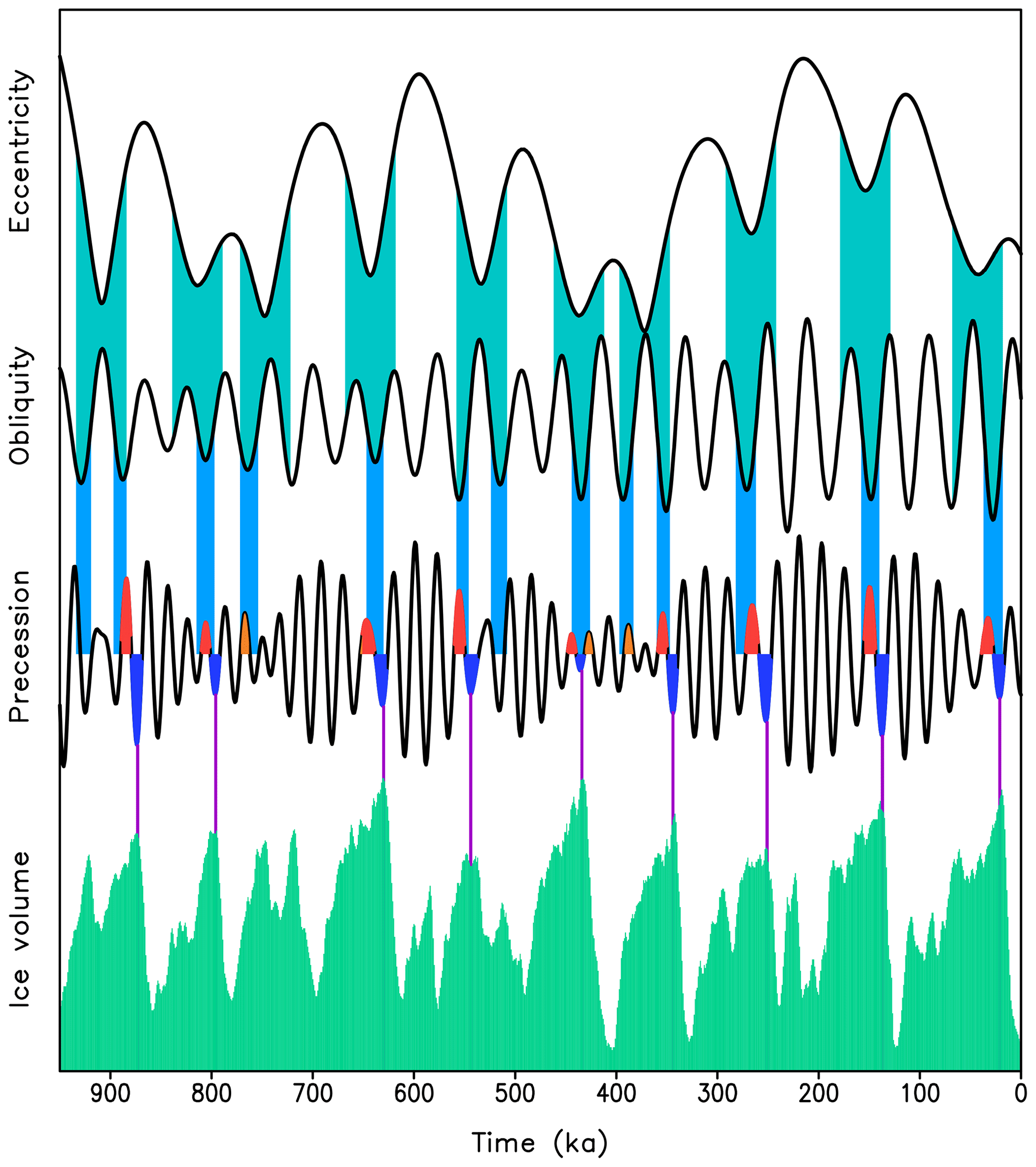
Figure 14A simple rule to determine the timing of glacial terminations. Grey shaded areas correspond to periods of low eccentricity and light blue to the periods of low obliquity during low eccentricity; red shading on the precession forcing curve highlights positive precession anomalies satisfying GMT criteria, and blue shading corresponds to following precession minima during which critical ice volume was reached (purple vertical line), and deglaciations start soon after these insolation minima. Orange shading on the precession curve corresponds to “false” positives, i.e., the cases when conditions of the termination rule are met, but they occurred earlier than 60 kyr after the previous termination. The lower curve is the LR04 benthic δ18O stack.
4.13 Short summary of GMT
According to the GMT, Quaternary glacial cycles represent the direct, strongly nonlinear response of the Earth system to variations of summer insolation in boreal latitudes of the Northern Hemisphere. This nonlinear response to orbital forcing is strongly modified and amplified by several processes and feedbacks. The existence of Quaternary glacial cycles, especially the strongly asymmetric late Quaternary cycles, is a peculiar and possibly absolutely unique feature of the current Earth system “configuration”. This explains significant difficulties in modeling and understanding Quaternary climate dynamics.
The onset of Quaternary glacial cycles was preconditioned by changes in the Earth's geography due to continental drift and by a gradual lowering of CO2 concentration, which eventually brought the Earth system into the state when insolation variations caused regular glaciations of the Northern Hemisphere. Before ca. 1 Ma, medium-amplitude glacial cycles terminated each time positive insolation anomalies due to precession and obliquity components of orbital forcing were in phase, which led to the dominance of obliquity (41 kyr) periodicity. The precession component of orbital forcing also played an essential role in driving early Quaternary glacial cycles, even if this periodicity is not detected in global ice volume reconstructions.
Gradual removal of terrestrial sediments from the northern continents by glacial erosion processes brought the Earth system into a new regime of operation when the dominant periodicity of glacial cycles shifted from 41 to 100 kyr. This regime change is explained by the fact that a large area of exposed rocks in Northern America combined with relatively low CO2 allowed medium-sized ice sheets to survive periods of high summer insolation and reach a much larger size and volume than the ice sheets of the early Quaternary. However, after reaching some critical state, a combination of several processes and feedbacks which are strongly dependent on the ice sheet size made such ice sheets unstable under boreal summer insolation rise. This led to rapid deglaciations, which explains the strong asymmetry of the late Quaternary glacial cycles. Since the critical ice sheet size can most likely be reached during periods of low eccentricity when one “positive” precession cycle is compensated for by a “negative” obliquity cycle, the glacial termination occurs during or after periods of low eccentricity. As a result, glacial cycles became phase-locked to short (100 kyr) eccentricity cycles, and this explains the sharp 100 kyr peak in the frequency spectra of the late Quaternary glacial cycles.
The central premise of the Milankovitch theory, namely that boreal summer insolation variations are the principal driver of Quaternary glacial cycles, was supported first by analysis of paleoclimate records which reveal the presence of all expected astronomical periodicities and then by modeling results which confirmed that these variations could cause waning and waxing of the continental ice sheets in the Northern Hemisphere. Thus, the Milankovitch theory in its original form has been confirmed, but paleoclimate records also revealed a number of important facts that were not known during Milankovitch's life and which his theory was not able to explain. The first one is that the late Quaternary is dominated by strongly asymmetric glacial cycles with the dominant 100 kyr cyclicity. The explanation for these cycles has attracted significant attention and continues to be regarded by some researchers as a challenge. In fact, the temporal dynamics of the late Quaternary glacial cycles, including the timing of glacial terminations and frequency spectra of climate variability, have already been successfully reproduced with a number of climate–ice models of different complexity ranging from simple 1-D models to a comprehensive Earth system model. In these model simulations, the dominant peak at 100 kyr periodicity in the frequency spectrum of ice volume is explained by the phase locking of long glacial cycles of the late Quaternary to 100 kyr eccentricity cycles. The eccentricity, in this case, serves as a pacemaker for the precession- and obliquity-driven glacial cycles, and the minuscule changes in global annual mean insolation associated with eccentricity cycles play no role here. The real forcing of glacial cycles is large (50–100 W m−2) changes in boreal summer insolation with precession and obliquity periods.
The idea that 100 kyr cyclicity originates from some strongly nonlinear response of the Earth system to the amplitude modulation of the precessional component of orbital forcing by the eccentricity, of course, is not new. However, it is important to emphasize that the late Quaternary glacial cycles cannot be explained simply by a nonlinear response because an arbitrary nonlinear response to orbital forcing should contain all eccentricity periodicities (95, 124, 400 kyr) as in the case of the Imbrie and Imbrie model, for example. In reality, only a single sharp peak at ca. 100 kyr is observed in the late Quaternary ice volume frequency spectrum. Thus, explaining paleoclimate records requires a very special type of nonlinearity. A number of simple and comprehensive models possess such nonlinearity and are thus able to reproduce the late Quaternary glacial cycles in good agreement with the paleodata. One of the main tasks of the GMT is to explain how such nonlinear responses originate from known processes and feedbacks operating in the Earth system, in particular what determines the critical size of the Northern Hemisphere ice sheets by reaching which they rapidly melt and disintegrate in response to rising boreal summer insolation. Understanding which processes in the Earth system explain such a response is one of the main challenges of contemporary Quaternary climate dynamics. The mechanism of this instability, named a domino effect by analogy with a simple mechanical system, is discussed above and based on the results of CLIMBER-2 and several other studies. Due to the complexity of the processes associated with glacial terminations and the absence of their analogies in present-day climate, a better understanding of the mechanism of glacial terminations requires further studies with comprehensive ESMs.
The processes which convert the seasonal and regional changes in insolation into global climate changes are now reasonably understood, and the Arrhenius idea about the role of CO2 in ice ages is confirmed. Modeling studies show that the lowering of CO2 by ca. 100 ppm, reinforced by CH4 and N2O drops, explains about half of the maximum glacial cooling, currently estimated at 5–6 ∘C, while the rest is attributed primarily to ice sheet expansion and sea level drop. It has been shown that CO2 also plays an important role in amplifying glacial cycles. This aspect of glacial cycles is still lacking a satisfactory explanation. Most studies to date were devoted to simulations of the low CO2 level at the LGM, and the CO2 radiative forcing has been prescribed in such studies. While such simulations are useful for testing the capability of modern ESMs to reproduce the carbon cycle response to glacial climate forcings, they do not answer the question of how the ice sheet–climate–carbon cycle feedback loops operated during the late Quaternary. The “stew” of the processes playing a role in glacial–interglacial CO2 variability has been discussed but still remains tentative and requires further studies with comprehensive Earth system models.
Another widely discussed challenge for the GMT is the nature of the 41 kyr world and the mechanism of the MPT. The difference between the early Quaternary 41 kyr world and the late Quaternary 100 kyr worlds can be solely explained by a gradual increase in the critical size of the ice sheets. As a result, glacial cycles, which are initially locked to obliquity cycles, became locked to the shortest eccentricity cycle. The most straightforward explanation for the increase in critical size is the removal of terrestrial sediments from the northern continents by glacial erosion. This mechanism alone allows reproducing the relatively sharp transition from the 41 to 100 kyr world in the models. The only obvious discrepancy with reality is that in all model simulations, the 41 kyr world contains a clear precession presence, while paleoclimate proxies usually show very little of such presence. The explanations for the lack of precession in the 41 kyr world range from physical mechanisms (antiphase response to the precession of the ice sheets in the Northern and Southern Hemisphere) to interpretation problems (much larger contribution to δ18O temperature signal) or some problems with the processing of paleoclimate data (like orbital tuning). In any case, this is an interesting but not critical issue for understanding how the Earth system responds to orbital forcing.
A comprehensive understanding of the mechanism of Quaternary climate variability still represents a formidable scientific challenge since this is a genuinely multidisciplinary problem. It is additionally complicated by the fact that present-day observational data provide insufficient constraints on the models used for paleoclimate studies, while paleoclimate records usually contain only indirect and incomplete information about past climate changes. Nevertheless, almost a century after the publication of Milankovitch's fundamental work, a framework for the generalized Milankovitch theory has emerged.
A1 Different metrics for orbital forcing
As shown for the first time by Milutin Milankovitch, changes in eccentricity, obliquity, and precession cause the substantial redistribution of insolation between latitudes and seasons. The comprehensive visualization of orbital forcing requires a 3-D plot (latitude – day of the year – time in years before or after present), which is impractical. Instead, different metrics for the orbital forcing were proposed. Milutin Milankovitch used the so-called caloric summer half-year insolation as a metric for orbital forcing, i.e., insolation integrated over the half-year with the highest insolation. In post-Milankovitch times, it became common to use June or July insolation at 65∘ N (e.g., Berger, 1978), although caloric half-year insolation is also used (e.g., Tzedakis et al., 2017). It is important to realize that using the modern calendar for defining orbital forcing on orbital timescales is problematic because the same calendar month in different years corresponds to different Earth positions relative to the perihelion and aphelion (e.g., Kutzbach and Gallimore, 1988). This is why it is advisable to define the metric for orbital forcing in a way that does not depend on the choice of calendar. Examples for such definitions are maximum summer insolation used in this paper or insolation averaged over a certain period of time, e.g., caloric half-year insolation originally used by Milankovitch. Examples of different insolation curves for 65∘ N are shown in Fig. A1.
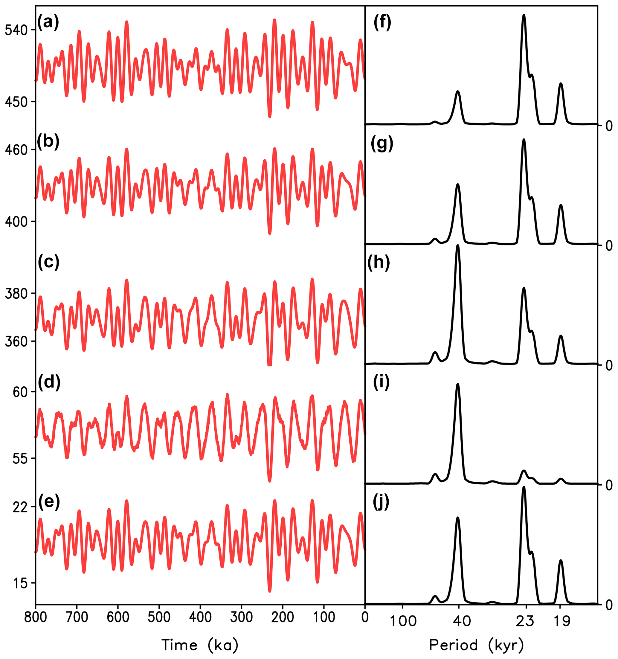
Figure A1Different proxies for orbital forcing. (a–e) Insolation at 65∘ N during the past 800 kyr and (f–j) corresponding frequency spectra. (a, f) Maximum summer insolation; (b, g) insolation averaged over 4 months with the highest insolation; (c, h) insolation averaged over 6 months with the highest insolation (the equivalent of caloric half-year energy but in different units); (d, i) “summer energy” computed according to Huybers (2006); (e, j) summer energy computed according to Eq. (A1). Insolation (a–c) is in W m−2, and summer energy (d, e) is in KJ. Frequency spectra are in arbitrary units.
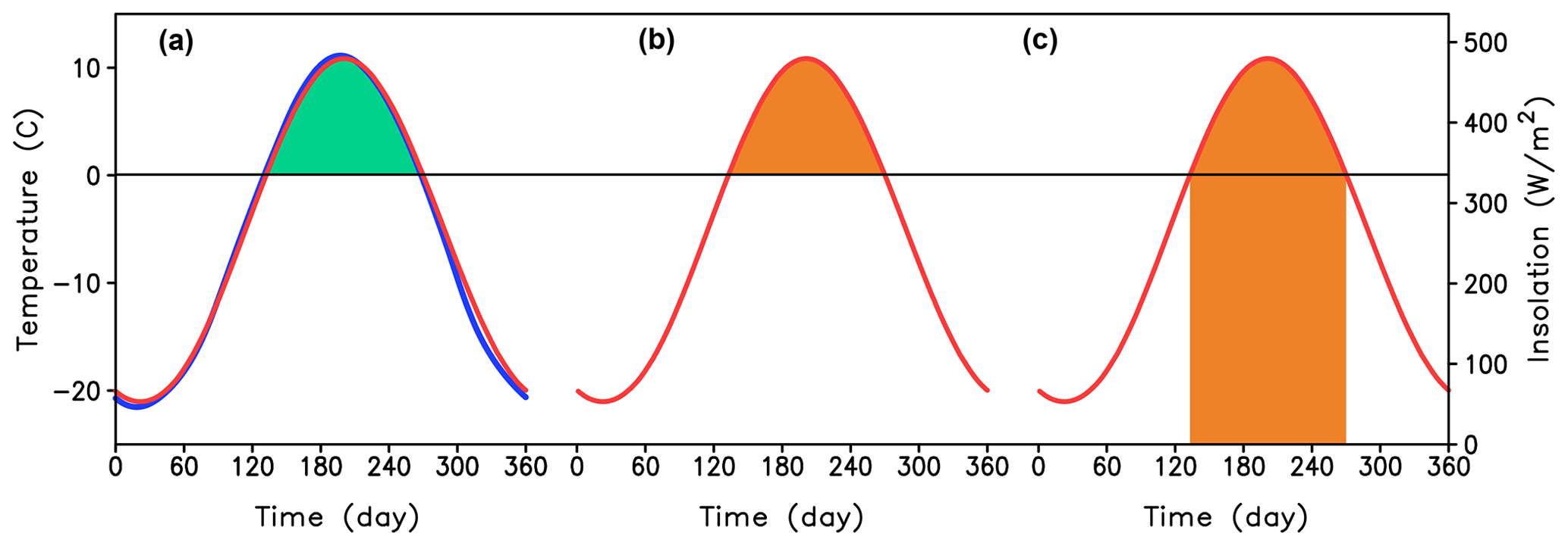
Figure A2Present temperature and insolation curves at 65∘ N and different definitions of “summer energy”. (a) Seasonal surface air temperature variation over land (blue) and insolation shifted by 30 d (red). The green area below the temperature curves represents the positive degree day index. (b) The orange area here represents an analogy for the positive degree days. The evolution of this characteristic is shown in Fig. A1e. This is a correct definition of summer energy. (c) The definition of summer energy according to Huybers (2006) is shown in Fig. A1d. The horizontal axis is the time of year in days.
Experiments with the CLIMBER-2 model show that during the late Quaternary, the rate of changes () in the Northern Hemisphere ice volume, which is primarily related to the surface mass balance of ice sheets, is most correlated with the maximum summer insolation at 65∘ N. When performing the same analysis but for reconstructed global sea level (Spratt and Lisiecki, 2016), which represents the global ice volume, the best correlation is found for the 65∘ N insolation average over the 4 months with the highest insolation (i.e., roughly MJJA). However, as Fig. A1 shows, the difference between maximum summer insolation and 4-month insolation is relatively small in obliquity and precession relative contribution. It is thus important to note that neither our model nor data suggest that caloric summer half-year insolation is the best proxy for orbital forcing. This can be explained by the fact that most of the ice melt (both at present and during glacial cycles) occurs only during a few summer months. Both precession and obliquity play essential roles in all computed insolation curves. The quantitative difference is that for the caloric half-year insolation, the contributions of precession and obliquity are comparable most of the time. In contrast, for the maximum summer insolation, the obliquity component is comparable with precession only during periods of a relatively low eccentricity.
However, there is one metric of orbital forcing which contains very little precession variability and is often used for the interpretation of paleoclimate records. This is the so-called “integrated summer insolation” proposed by Huybers (2006) and which is defined as
where Ii is the daily insolation at 65∘ N and I0 is a constant value set to 275 W m−2 in Huybers (2006). This choice of the metric for orbital forcing is justified by the fact that seasonal variations of temperature over land and insolation are rather similar (with about a 1-month lag of temperature behind insolation) and that the melt rate of ice sheets is often parameterized through the so-called positive degree day index defined as for all daily temperatures Ti>0 (Fig. A2) . However, to correctly translate insolation into PDD index, one should consider the fact that for an arbitrary temperature scale, PDD should be defined as . T0=0 ∘C only for the Celsius temperature scale, and thus T0 can be omitted in the formula for PDD. However, for example, in the case of the Kelvin temperature scale T0=273.15 K. Therefore, PDD should be expressed through the insolation as
Obviously, this formulation is significantly different from the original integrated summer insolation (compare Fig. A1d and e), and similarly to other metrics for orbital forcing it contains a strong precession signal. Thus, none of the physically meaningful metrics for orbital forcing are free of a strong precession component, which is important for discussions of the nature of the 41 kyr world.
A2 Imbrie and Imbrie conceptual model
One of the first and most well-known conceptual models of late Quaternary glacial cycles is the Imbrie and Imbrie (1980) model. This model has been applied for the orbital tuning of the widely used LR04 record (Lisiecki and Raymo, 2005). The model is represented by a single equation for global ice volume v (in arbitrary units):
where is the equilibrium volume for orbital forcing f, and the c1 value is constant. The relaxation timescale τk depends on the regime: k=1 if v>Ve, and k=2 if v<Ve. If τ1=τ2, the model is linear and its response to orbital forcing is similar to forcing itself with only obliquity and precession frequencies present. Using τ2 much larger than τ1, as in Imbrie and Imbrie (1980), makes the model nonlinear. The model performance is far from perfect (see, e.g., Paillard, 2001), and even for the optimal choice of model parameters, the correlation between modeled v and LR04 stack for the last 800 kyr does not exceed 0.6. Even more important is that the modeled ice volume variability has too much energy in the 400 kyr band and too little energy in the 100 kyr band (Fig. A3).
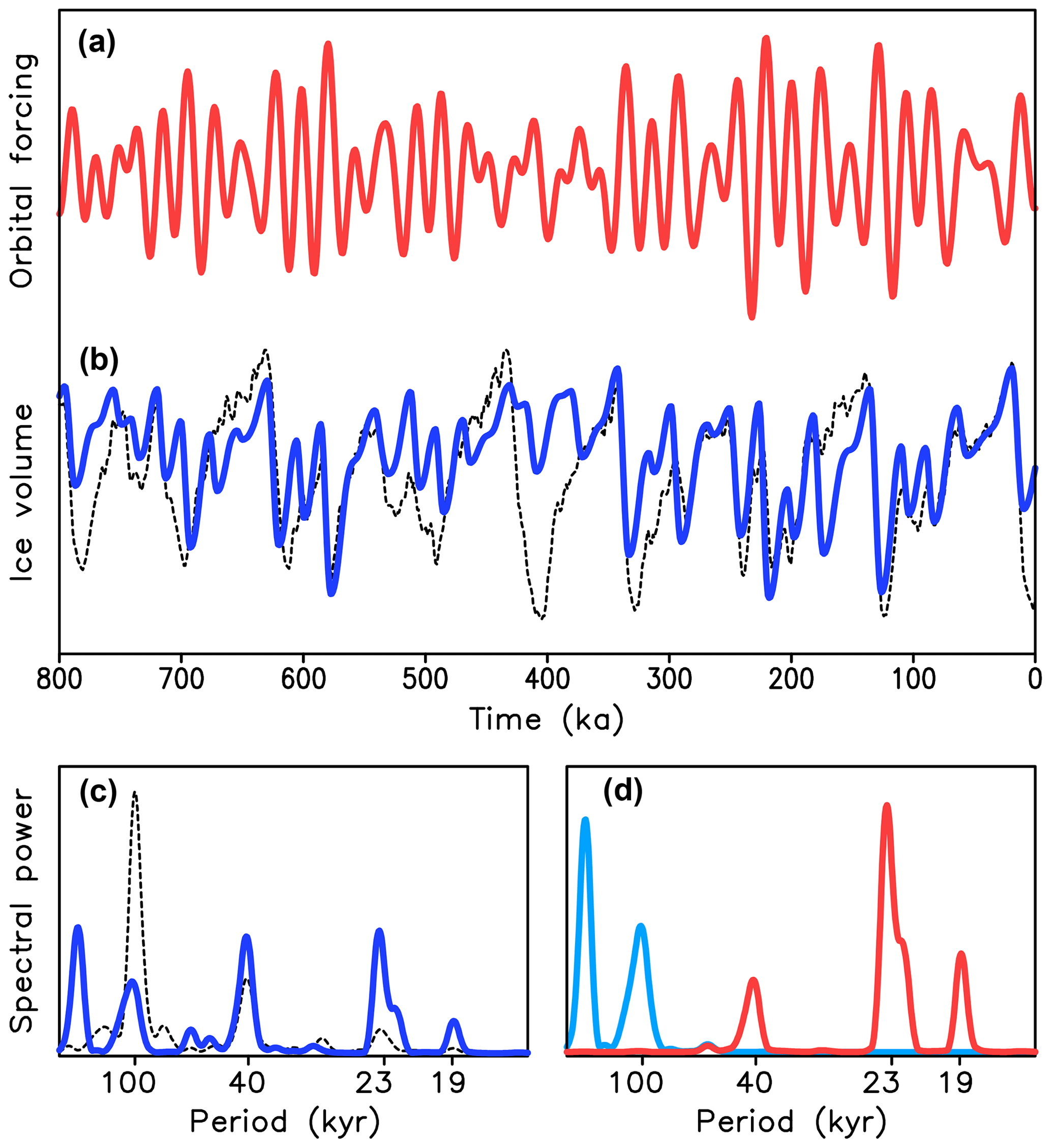
Figure A3Results of simulations of the last 800 kyr with the Imbrie and Imbrie (1980) model. (a) Orbital forcing; (b) simulated ice volume (solid) and LR04 stack (dashed); (c) frequency spectra of simulated ice volume (blue) and LR04 stack (dashed line); (d) frequency spectra of eccentricity (blue) and orbital forcing (red). Vertical scales are arbitrary.
A3 The rules for the timing of glacial terminations based on two or three obliquity cycles and effective energy
Huybers and Wunsch (2005) analyzed benthic δ18O records and concluded that glacial terminations of the late Quaternary were spaced in time by two or three obliquity cycles, while the link with precession and eccentricity was not found to be statistically significant. Later, Huybers (2009) admitted that precession has a role in glacial cycles, but the concept of “two or three obliquity cycles” remains rather popular. Indeed, there is a clear tendency for glacial terminations to occur during periods of positive obliquity anomalies, although the durations between individual terminations can deviate significantly from two (82) or three (123 kyr) obliquity cycles (see below). When rounding to the nearest integers, the last eight glacial cycles can be expressed in terms of obliquity periods as 2, 2, 2, 3, 2, 2, 3, and 3. The average number of obliquity periods, 2.6, multiplied by obliquity periods gives 97 kyr, which is very close to the observed dominant periodicity of late Quaternary glacial cycles. But it is also clear that the probability of getting the correct sequence of “2” and “3” by random choice is , which is a rather low probability, while the models used in this study demonstrate that the timing of all glacial terminations of the late Quaternary is relatively robust. Even more problematic for the “two or three” hypothesis is that if this hypothesis is correct, then the duration of individual glacial cycles should cluster around 82 and 123 kyr with equal probabilities of being longer or shorter: 2(3)⋅41 kyr. In fact, durations of the last eight glacial cycles are rather uniformly distributed between ca. 80 and 120 ka, with five of eight glacial cycles having durations between 90 and 110 kyr, i.e., closer to 100 kyr than to two or three obliquity cycles (e.g., Konijnendijk et al., 2015).
The term effective energy was introduced by Tzedakis et al. (2017). According to this paper, terminations (during the last 600 kyr) occur when the effective energy defined as Ipeak+b(Δt) exceeds 6.412 GJ m−2. Here Ipeak is the magnitude of the maximum caloric half-year summer insolation at 65∘ N, Δt is the time since previous deglaciation, and b is a constant. This rule for glacial terminations implies that the Earth system somehow “knows” in advance whether the effective energy will cross the threshold value, which usually happens well after the beginning of terminations. In some cases (for example, for the penultimate glaciation), glacial terminations have been completed even before the maximum effective energy has been reached. How can this rule and a somewhat similar one described in Huybers (2011) be reconciled with the GMT, which “predicts” terminations not based on the magnitude of insolation maxima but rather by the timing when ice volume exceeds the critical threshold? In fact, it can be shown that, although these rules are based on completely different physical concepts, they indeed give similar timing of glacial terminations. The rule based on “efficient energy” formulated by Tzedakis et al. (2017) implies that glacial terminations occur only during maxima of caloric half-year summer insolation that are above the average value of insolation maxima which occurred close to each obliquity maxima. This can only happen if both precession and obliquity components of summer insolation are positive, and the eccentricity is also above average. Since the period of obliquity (41 kyr) is approximately twice as long as the period of precession and is comparable with half of a 100 kyr eccentricity period, it is highly probable that the previous positive precessional maximum occurred during the obliquity minimum and eccentricity was below average. But this is precisely the condition for reaching the critical ice volume in the GMT. Thus, with the appropriate initial conditions, the Tzedakis et al. (2017) rule produces the same (or similar) sequence of terminations as the GMT.
A4 Model 2
Model 2 is a one-equation conceptual model aimed at reproducing the principal CLIMBER-2 results. It is derived using several assumptions, among which is that total accumulation (mass gain of ice sheets) G is proportional to the ice sheet area, but since the latter closely followed global ice volume v (e.g., Ganopolski et al., 2010), the total accumulation is parameterized as
The total mass loss (including both surface and basal melt, as well as ice calving into the ocean) L is a nonlinear function of ice volume. It also includes an additional term proportional to the rate of ice volume change:
The last term is nonzero only for ice sheet decay, i.e., δ=1 if and δ=0 if . The value is the memory term defined as the average ice volume over the previous N kiloyears. This term is crucial to simulate glacial terminations through the domino effect. The effect of insolation M (which can be positive and negative) is accounted for through a linear function of orbital forcing f (anomaly of maximum summer insolation at 65∘ N, see Sect. 4):
where , and f1 is the model parameter. Of course, orbital forcing can contribute to both “mass loss” and gain and is treated here separately just for convenience.
Temporal evolution of global ice volume (in normalized units) is thus described by the equation
where , and .
To prevent the denominator in Eq. (A4) from approaching zero and subsequently becoming negative, it is additionally required that D≥ε. In these equations, a, b, c, g, ε, and N are model parameters (see Table 1). Mathematically this equation is not much more complex than the governing equation of Model 3, but it has a clearer physical meaning. At the same time, it is easy to show that Model 3 is a simplified version of Model 2. The equilibrium solution of Eq. (A7) for ice volume Ve (see also Fig. A4) is
This is a rotated counterclockwise parabolic curve, identical to the equilibrium solutions of Model 3 (Fig. 4).
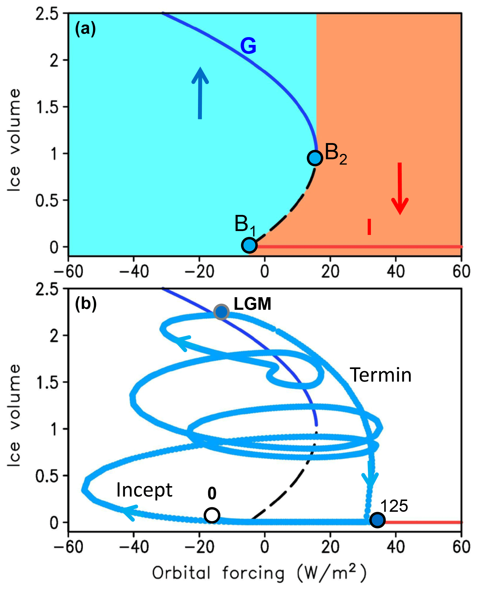
Figure A4(a) Stability diagram for Model 2. Notations are the same as in Fig. 3. (b) Trajectory of the system described by Model 2 in the phase space of orbital forcing-ice volume for the last 125 kyr.
As it follows directly from Eq. (A7), growth of ice volume from zero (glacial inception) can only occur for , i.e., , which means that the value f1 (bifurcation point B1) has the same meaning as f1 in Model 3. The position of the second bifurcation point B2 in the phase space of orbital forcing (the equivalent of f2 in Model 3) is defined as . Since the vertical scale of the equilibrium solution is defined by the combination of parameters a and b, the number of parameters can be reduced to six by setting . This gives the equilibrium solution Ve(f2)=1 for ice volume at the bifurcation point B2, which is the same as in Model 3. While Model 2 has qualitatively the same stability diagram as Model 3, it differs from the latter in that the timescale of relaxation towards the equilibrium solutions in Model 2 is not constant and depends on the position in the insolation-volume phase space. A typical relaxation timescale of Model 2 in the glaciation regime (i.e., when ) can be estimated as 2a−1, which, for the value of a given in Table 1, is ca. 27 kyr, i.e., is similar to the (constant) relaxation timescale of Model 3. In the case of glacial termination, the rate of ice loss increases by the factor D−1, which is an order of 10 when the memory term v* approaches the critical ice volume equal to g−1.
Figure A5 shows results of simulations of the last 800 kyr in comparison with paleoclimate reconstructions for the optimal set of model parameters (see Table 1). Correlation between the model and LR04 stack is 0.8, which is similar to Model 3. As in the case of Model 3, the “termination” regime described by the term D in Eq. (A7) is absolutely crucial. Without this term, Model 2 simulates a weakly nonlinear response with the presence of all Milankovitch frequencies, similar to the one-regime version of Model 3 and the Imbrie and Imbrie model. Compared to Model 3, Model 2 does a better job for the pre-MBT glacial cycles but, similarly to CLIMBER-2 (Willeit et al., 2019), has a problem with simulating long interglacial MIS 11, which Model 3 does not. This is explained by a very weak orbital forcing which triggered Termination V (transition to MIS 11 interglacial). Since in Model 3, the transition to a glaciation regime does not depend on the value of orbital forcing (it should only be growing and positive), it is easier to simulate the correct timing of Termination V with Model 3 than with Model 2, where the magnitude of orbital forcing matters. After MIS 11, Model 2 performs well for a rather broad range of model parameters and the maximum correlation between simulated ice volume and LR04 for this time interval reaches 0.9. Note that the extended version of Model 2, which also includes equations for CO2 and global temperature, has been developed and applied to future glacial cycle simulations in Talento and Ganopolski (2021).
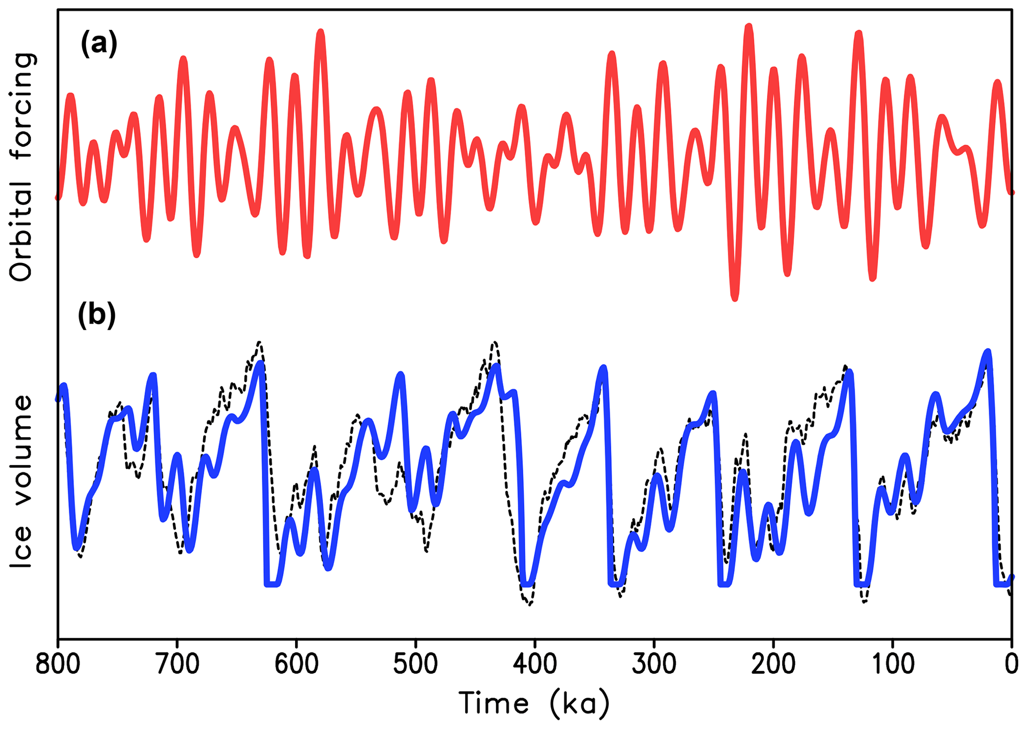
A5 The role of obliquity in a 100 kyr world
Since obliquity completely dominates δ18O records of the 41 kyr world, it is natural to assume that obliquity also plays an essential role in a 100 kyr world. However, the experiments performed with the CLIMBER-2 model (Ganopolski and Calov, 2011) demonstrate that the dominant 100 kyr periodicity is present even when the obliquity component is completely excluded from the orbital forcing. At the same time, this periodicity cannot be simulated without eccentricity modulation of the precession component. Model 3 demonstrates the same behavior: when forced by the precession component of orbital forcing alone, it simulates a strong maximum in the frequency spectrum at 100 kyr for a broad range of the model parameter vc. The presence of obliquity affects the timing of some glacial terminations, and therefore the duration of the individual glacial cycles, but not the dominant periodicity (Fig. A6). In the absence of the obliquity component, the durations of individual glacial cycles cluster around four and five precession periods (i.e., ca. 90 and 100 kyr) rather than two and three obliquity periods. Similar to CLIMBER-2 (Ganopolski and Calov, 2011), in Model 3 with obliquity-free orbital forcing, more energy in frequency spectra is seen in the 400 kyr band than in the case of realistic orbital forcing. However, the amount of energy in the 400 kyr band, unlike the 100 kyr, is strongly dependent on the choice of model parameters. In short, model simulations show that, although the obliquity component of orbital forcing plays an important role in climate variability during both the 41 and 100 kyr worlds, it has nothing to do with the dominant 100 kyr periodicity of the glacial cycles of the late Quaternary.
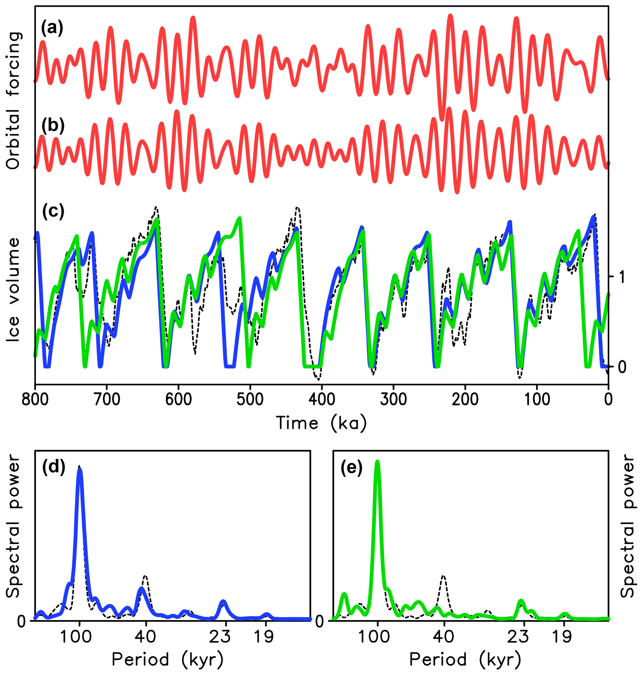
Figure A6Results of simulations of the last 800 kyr with Model 3 with and without an obliquity component in orbital forcing. (a) Full orbital forcing; (b) orbital forcing without an obliquity component; (c) simulated ice volume with obliquity (blue) and without an obliquity component (green), as well as the LR04 stack (dashed); (d) spectra of simulated ice volume with an obliquity component (blue) and LR04 stack (dashed line); (e) spectra of simulated ice volume without an obliquity component (green) and LR04 stack (dashed line).
A6 Orbital tuning and the absence of precession in early Quaternary records
One of the potential causes of the absence of precession in the δ18O spectra during the early Quaternary is that these time series are often orbitally tuned using obliquity as the target (e.g., Lisiecki and Raymo 2005). Since obliquity is the dominant frequency in the early Quaternary ice volume variations, such a choice seems to be reasonable. However, in the case of a strongly nonlinear system, tuning the age model to maximize one frequency may lead to the suppression of another one. This is illustrated by Fig. A7, where the results of model simulation described in Sect. 3 and shown in Fig. 10b have been “tuned to obliquity”. Simulated ice volume already has a strong obliquity component (Fig. A4c) and the correlation between simulated volume and (negative) obliquity anomaly shifted by 5000 years is about 0.5. However, the spectrum also has pronounced precession maxima. To mimic the potential impact of orbital tuning on the frequency spectrum, the “age” of modeled ice volume has been modified to maximize correlation with obliquity. This time correction satisfies two criteria similar to those used in the actual orbital tuning: (i) the initial (in this case, real) age has not been changed by more than 10 kyr, and (ii) the original timescale was not stretched or squeezed by more than a factor of 2 at any time. Figure A7c shows the change in the original age, which gives the higher correlation between “tuned” volume and the target (obliquity). Now, this correlation reaches 0.65, practically the same value as the correlation between LR04 stack and obliquity (0.66). As Fig. A7 shows, this “tuning” slightly increases spectral energy in the obliquity band but causes a nearly complete disappearance of precession components (Fig. A7e).
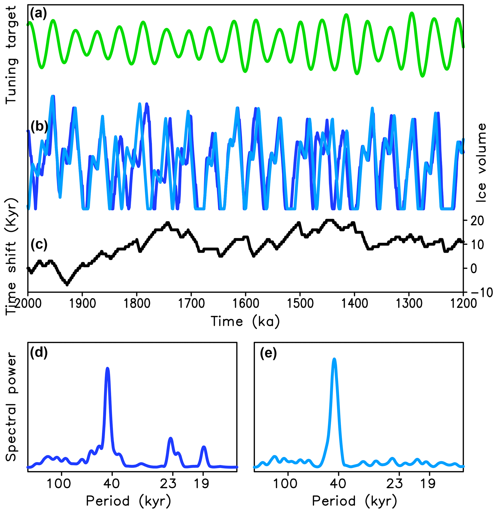
Figure A7“Minimal orbital tuning”. (a) Tuning target: negative anomaly of obliquity shifted by 5000 kyr; (b) simulated and “tuned” ice volume; (c) time shift for the tuned time series; (d, e) corresponding frequency spectra. The dark blue line is the original simulation of the 41 kyr world with Model 3 (the same as in Fig. 8), and the light blue line shows optimally tuned Model 3 simulations. The vertical scales in (d) and (e) are the same.
The source codes and the output of the model simulations are available on request from the author.
The author has declared that there are no competing interests.
Publisher's note: Copernicus Publications remains neutral with regard to jurisdictional claims made in the text, published maps, institutional affiliations, or any other geographical representation in this paper. While Copernicus Publications makes every effort to include appropriate place names, the final responsibility lies with the authors.
This article is part of the special issue “A century of Milankovic's theory of climate changes: achievements and challenges (NPG/CP inter-journal SI)”. It is not associated with a conference.
The author thanks Michel Crucifix, Martin Claussen, and an anonymous reviewer for valuable comments and suggestions, as well as Mikhail Verbitsky, Matteo Willeit, and Christine Kaufhold for helpful discussions.
This paper was edited by Martin Claussen and reviewed by Michel Crucifix and one anonymous referee.
Abe-Ouchi, A., Saito, F., Kawamura, K., Raymo, M. E., Okuno, J., Takahashi, K., and Blatter, H.: Insolation-driven 100,000-year glacial cycles and hysteresis of ice-sheet volume, Nature, 500, 190–194, https://doi.org/10.1038/nature12374, 2013.
Adhémar, J. A.: Revolutions de la Mer: Deluges Periodiques, Carilian-Goeury et V. Dalmont, Paris, 1842.
Albani, S., Balkanski, Y., Mahowald, N., Winckler, G., Maggi, V., and Delmonte, B.: Aerosol-climate interactions during the Last Glacial Maximum, Curr. Clim. Change Rep., 4, 99–114, https://doi.org/10.1007/s40641-018-0100-7, 2018.
Andrews, J. T.: The Wisconsin Laurentide ice sheet: dispersal centers, problems of rates of retreat, and climatic implications, Arct. Alp. Res., 5, 185–199, https://doi.org/10.1080/00040851.1973.12003700, 1973.
Archer, D. and Ganopolski, A.: A movable trigger: Fossil fuel CO2 and the onset of the next glaciation, Geochem. Geophy. Geosy., 6, 1–7, https://doi.org/10.1029/2004gc000891, 2005.
Archer, D., Winguth, A., Lea, D., and Mahowald, N.: What caused the glacial/interglacial atmospheric pCO2 cycles?, Rev. Geophys., 38, 159–189, https://doi.org/10.1029/1999RG000066, 2000.
Arrhenius, S.: On the influence of carbonic acid in the air upon the temperature of the ground, Philos. Mag., 41, 237–275, 1896.
Ashwin, P., Camp, C. D., and von der Heydt, A. S.: Chaotic and non-chaotic response to quasiperiodic forcing: Limits to predictability of ice ages paced by Milankovitch forcing, Dynam. Stat. Clim. Syst., 3, 1–20, https://doi.org/10.1093/climsys/dzy002, 2018.
Barker, S., Starr, A., van der Lubbe, J., Doughty, A., Knorr, G., Conn, S., Lordsmith, S., Owen, L., Nederbragt, A., Hemming, S., and Hall, I.: Persistent influence of precession on northern ice sheet variability since the early Pleistocene, Science, 376, 961–967, https://doi.org/10.1126/science.abm4033, 2022.
Bauer, E. and Ganopolski, A.: Sensitivity simulations with direct shortwave radiative forcing by aeolian dust during glacial cycles, Clim. Past, 10, 1333–1348, https://doi.org/10.5194/cp-10-1333-2014, 2014.
Benzi, R., Parisi, G., Sutera, A., and Vulpiani, A.: Stochastic resonance in climatic change, Tellus, 34, 10–16, 1982.
Berends, C. J., Köhler, P., Lourens, L. J., and van de Wal, R. S. W.: On the cause of the mid-Pleistocene transition, Rev. Geophys., 59, e2020RG000727, https://doi.org/10.1029/2020RG000727, 2021.
Berger, A.: Obliquity and general precession for the last 5 000 000 years, Astron. Astrophys., 51, 127–135, 1976.
Berger, A.: Long-term variations of daily insolation and quaternary climatic changes, J. Atmos. Sci., 35, 2362–2367, https://doi.org/10.1175/1520-0469(1978)035<2362:Ltvodi>2.0.Co;2, 1978.
Berger, A.: Milankovitch theory and climate, Rev. Geophys., 26, 624–657, https://doi.org/10.1029/RG026i004p00624, 1988.
Berger, A.: A Brief History of the Astronomical Theories of Paleoclimates, in: Climate Change, edited by: Berger, A., Mesinger, F., and Šijački, D., Springer-Verlag, Wien, 107–129, https://doi.org/10.1007/978-3-7091-0973-1, 2012.
Berger, A.: Milankovitch, the father of paleoclimate modeling, Clim. Past, 17, 1727–1733, https://doi.org/10.5194/cp-17-1727-2021, 2021.
Berger, A. and Loutre, M. F.: Modeling the 100-kyr glacial-interglacial cycles, Global Planet. Change, 72, 275–281, https://doi.org/10.1016/j.gloplacha.2010.01.003, 2010.
Berger, A., Li, X. S., and Loutre, M. F.: Modelling northern hemisphere ice volume over the last 3 Ma, Quaternary Sci. Rev., 18, 1–11, https://doi.org/10.1016/s0277-3791(98)00033-x, 1999.
Bouttes, N., Paillard, D., Roche, D. M., Waelbroeck, C., Kageyama, M., Lourantou, A., Michel, E., and Bopp, L.: Impact of oceanic processes on the carbon cycle during the last termination, Clim. Past, 8, 149–170, https://doi.org/10.5194/cp-8-149-2012, 2012.
Braconnot, P., Otto-Bliesner, B., Harrison, S., Joussaume, S., Peterchmitt, J. Y., Abe-Ouchi, A., Crucifix, M., Driesschaert, E., Fichefet, T., Hewitt, C. D., Kageyama, M., Kitoh, A., Laine, A., Loutre, M. F., Marti, O., Merkel, U., Ramstein, G., Valdes, P., Weber, S. L., Yu, Y., and Zhao, Y.: Results of PMIP2 coupled simulations of the Mid-Holocene and Last Glacial Maximum – Part 1: experiments and large-scale features, Clim. Past., 3, 261–277, https://doi.org/10.5194/cp-3-261-2007, 2007.
Brendryen, J., Haflidason, H., Yokoyama, Y., Haaga, K. A., and Hannisdal, B.: Eurasian Ice Sheet collapse was a major source of Meltwater Pulse 1A 14,600 years ago, Nat. Geosci., 13, 363–368, https://doi.org/10.1038/s41561-020-0567-4, 2020.
Briggs, R. D., Pollard, D., and Tarasov, L.: A data-constrained large ensemble analysis of Antarctic evolution since the Eemian, Quaternary Sci. Rev., 103, 91–115, https://doi.org/10.1016/j.quascirev.2014.09.003, 2014.
Broecker, W. S. and Van Donk, J.: Insolation changes, ice volumes, and the O18 record in deep-sea cores, Rev. Geophys., 8, 169–198, https://doi.org/10.1029/RG008i001p00169, 1970.
Brovkin, V., Ganopolski, A., Archer, D., and Rahmstorf, S.: Lowering of glacial atmospheric CO2 in response to changes in oceanic circulation and marine biogeochemistry, Paleoceanography, 22, PA4202, https://doi.org/10.1029/2006pa001380, 2007.
Brovkin, V., Ganopolski, A., Archer, D., and Munhoven, G.: Glacial CO2 cycle as a succession of key physical and biogeochemical processes, Clim. Past., 8, 251–264, https://doi.org/10.5194/cp-8-251-2012, 2012.
Brückner, E., Köppen, W., and Wegener, A.: Über die Klimate der geologischen Vorzeit, Z. Gletscherkd., 14, 149–169, 1925.
Budyko, M. I.: Future climate, Trans. Am. Geophys. Union, 53, 868–874, https://doi.org/10.1029/EO053i010p00868, 1972.
Calder, N.: Arithmetic of ice ages, Nature, 252, 216–218, https://doi.org/10.1038/252216a0, 1974.
Calov, R. and Ganopolski, A.: Multistability and hysteresis in the climate-cryosphere system under orbital forcing, Geophys. Res. Lett., 32, L21717, https://doi.org/10.1029/2005GL024518, 2005.
Calov, R., Ganopolski, A., Claussen, M., Petoukhov, V., and Greve, R.: Transient simulation of the last glacial inception with an atmosphere-ocean-vegetation-ice sheet. Part I: Glacial inception as a bifurcation of the climate system, Clim. Dynam., 24, 545–561, 2005a.
Calov, R., Ganopolski, A., Petoukhov, V., Claussen, M., Brovkin, V., and Kubatzki, C.: Transient simulation of the last glacial inception. Part II: sensitivity and feedback analysis, Clim. Dynam., 24, 563–576, https://doi.org/10.1007/s00382-005-0008-5, 2005b.
Cane, M. A. and Molnar, P.: Closing of the Indonesian seaway as a precursor to east African aridircation around 3–4 million years ago, Nature, 411, 157–162, https://doi.org/10.1038/35075500, 2001.
Chalk, T. B., Hain, M. P., Foster, G. L., Rohling, E. J., Sexton, P. F., Badger, M. P. S., Cherry, S. G., Hasenfratz, A. P., Haug, G. H., Jaccard, S. L., Martinez-Garcia, A., Palike, H., Pancost, R. D., and Wilson, P. A.: Causes of ice age intensification across the Mid-Pleistocene Transition, P. Natl. Acad. Sci. USA, 114, 13114–13119, https://doi.org/10.1073/pnas.1702143114, 2017.
Charbit, S., Ritz, C., Philippon, G., Peyaud, V., and Kageyama, M.: Numerical reconstructions of the Northern Hemisphere ice sheets through the last glacial-interglacial cycle, Clim. Past., 3, 15–37, https://doi.org/10.5194/cp-3-15-2007, 2007.
Choudhury, D., Timmermann, A., Schloesser, F., Heinemann, M., and Pollard, D.: Simulating Marine Isotope Stage 7 with a coupled climate–ice sheet model, Clim. Past, 16, 2183–2201, https://doi.org/10.5194/cp-16-2183-2020, 2020.
Clark, P. U. and Pollard, D.: Origin of the Middle Pleistocene Transition by ice sheet erosion of regolith, Paleoceanography, 13, 1–9, 1998.
Claussen, M., Mysak, L. A., Weaver, A. J., Crucifix, M., Fichefet, T., Loutre, M. F., Weber, S. L., Alcamo, J., Alexeev, V. A., Berger, A., Calov, R., Ganopolski, A., Goosse, H., Lohmann, G., Lunkeit, F., Mokhov, I., Petoukhov, V., Stone, P., and Wang, Z.: Earth system models of intermediate complexity: closing the gap in the spectrum of climate system models, Clim. Dynam., 18, 579–586, https://doi.org/10.1007/s00382-001-0200-1, 2002.
Claussen, M., Fohlmeister, J., Ganopolski, A., and Brovkin, V.: Vegetation dynamics amplifies precessional forcing, Geophys. Res. Lett., 33, L09709, https://doi.org/10.1029/2006GL026111, 2006.
Croll, J.: On the physical cause of the change of climate during geological epochs, Philos. Mag., 28, 121–137, 1864.
Crucifix, M.: Oscillators and relaxation phenomena in Pleistocene climate theory, Philos. T. Roy. Soc. A, 370, 1140–1165, https://doi.org/10.1098/rsta.2011.0315, 2012.
Crucifix, M.: Why could ice ages be unpredictable?, Clim. Past., 9, 2253–2267, https://doi.org/10.5194/cp-9-2253-2013, 2013.
Crucifix, M. and Hewitt, C. D.: Impact of vegetation changes on the dynamics of the atmosphere at the Last Glacial Maximum, Clim. Dynam., 25, 447–459, https://doi.org/10.1007/s00382-005-0013-8, 2005.
Dang, C., Brandt, R. E., and Warren, S. G.: Parameterizations for narrowband and broadband albedo of pure snow and snow containing mineral dust and black carbon, J. Geophys. Res.-Atmos., 120, 5446–5468, https://doi.org/10.1002/2014JD022646, 2015.
Daradich, A., Huybers, P., Mitrovica, J. X., Chan, N. H., and Austermann, J.: The influence of true polar wander on glacial inception in North America, Earth Planet. Sc. Lett., 461, 96–104, https://doi.org/10.1016/j.epsl.2016.12.036, 2017.
de Noblet, N. I., Prentice, I. C., Joussaume, S., Texier, D., Botta, A., and Haxeltine, A.: Possible role of atmosphere–biosphere interaction in triggering the last glaciation, Geophys. Res. Lett., 23, 3191–3194, 1996.
Dong, B. W. and Valdes, P. J.: Sensitivity studies of northern-hemisphere glaciation using an atmospheric general-circulation model, J. Climate, 8, 2471–2496, https://doi.org/10.1175/1520-0442(1995)008<2471:SSONHG>2.0.CO;2, 1995.
Elderfield, H., Ferretti, P., Greaves, M., Crowhurst, S., McCave, I. N., Hodell, D., and Piotrowski, A. M.: Evolution of Ocean Temperature and Ice Volume Through the Mid-Pleistocene Climate Transition, Science, 337, 704–709, https://doi.org/10.1126/science.1221294, 2012.
Emiliani, C.: Paleotemperature analysis of Caribbean cores P6304-8 and P6304-9 and a generalized temperature curve for the past 425,000 years, J. Geol., 74, 109–124, 1966.
Farmer, J. R., Honisch, B., Haynes, L. L., Kroon, D., Jung, S., Ford, H. L., Raymo, M. E., Jaume-Segui, M., Bell, D. B., Goldstein, S. L., Pena, L. D., Yehudai, M., and Kim, J.: Deep Atlantic Ocean carbon storage and the rise of 100,000-year glacial cycles, Nat. Geosci., 12, 355–360, https://doi.org/10.1038/s41561-019-0334-6, 2019.
Ford, H. L. and Raymo, M. E.: Regional and global signals in seawater δ18O records across the mid-Pleistocene transition, Geology, 48, 113–117, https://doi.org/10.1130/g46546.1, 2020.
Galbraith, E. and de Lavergne, C.: Response of a comprehensive climate model to a broad range of external forcings: relevance for deep ocean ventilation and the development of late Cenozoic ice ages, Clim. Dynam., 52, 653–679, 2019.
Ganopolski, A.: Glacial integrative modelling, Philos. T. Roy. Soc. Lond. A, 361, 1871–1883, https://doi.org/10.1098/rsta.2003.1246, 2003.
Ganopolski, A. and Brovkin, V.: Simulation of climate, ice sheets and CO2 evolution during the last four glacial cycles with an Earth system model of intermediate complexity, Clim. Past., 13, 1695–1716, https://doi.org/10.5194/cp-13-1695-2017, 2017.
Ganopolski, A. and Calov, R.: The role of orbital forcing, carbon dioxide and regolith in 100 kyr glacial cycles, Clim. Past., 7, 1415–1425, https://doi.org/10.5194/cp-7-1415-2011, 2011.
Ganopolski, A., Petoukhov, V., Rahmstorf, S., Brovkin, V., Claussen, M., Eliseev, A., and Kubatzki C.: CLIMBER-2: a climate system model of intermediate complexity. Part II: Model sensitivity, Clim. Dynam., 17, 735–751, 2001.
Ganopolski, A., Calov, R., and Claussen, M.: Simulation of the last glacial cycle with a coupled climate ice-sheet model of intermediate complexity, Clim. Past, 6, 229–244, https://doi.org/10.5194/cp-6-229-2010, 2010.
Ganopolski, A., Winkelmann, R., and Schellnhuber, H. J.: Critical insolation-CO2 relation for diagnosing past and future glacial inception, Nature, 529, 200–204, https://doi.org/10.1038/nature16494, 2016.
Gregoire, L. J., Valdes, P. J., and Payne, A. J.: The relative contribution of orbital forcing and greenhouse gases to the North American deglaciation, Geophys. Res. Lett., 42, 9970–9979, https://doi.org/10.1002/2015GL066005, 2015.
Gregory, J. M., Browne, O. J. H., Payne, A. J., Ridley, J. K., and Rutt, I. C.: Modelling large-scale ice-sheet-climate interactions following glacial inception, Clim. Past., 8, 1565–1580, https://doi.org/10.5194/cp-8-1565-2012, 2012.
Hargreaves, J. C., Abe-Ouchi, A., and Annan, J. D.: Linking glacial and future climates through an ensemble of GCM simulations, Clim. Past, 3, 77–87, https://doi.org/10.5194/cp-3-77-2007, 2007.
Hasenfratz, A. P., Jaccard, S. L., Martinez-Garcia, A., Sigman, D. M., Hodell, D. A., Vance, D., Bernasconi, S. M., Kleiven, H. F., Haumann, F. A., and Haug, G. H.: The residence time of Southern Ocean surface waters and the 100,000-year ice age cycle, Science, 363, 1080–1084, https://doi.org/10.1126/science.aat7067, 2019.
Haug, G. H. and Tiedemann, R.: Effect of the formation of the Isthmus of Panama on Atlantic Ocean thermohaline circulation, Nature, 393, 673–676, https://doi.org/10.1038/31447, 1998.
Haug, G. H., Ganopolski, A., Sigman, D. M., Rosell-Mele, A., Swann, G. E. A., Tiedemann, R., Jaccard, S. L., Bollmann, J., Maslin, M. A., Leng, M. J., and Eglinton, G.: North Pacific seasonality and the glaciation of North America 2.7 million years ago, Nature, 433, 821–825, 2005.
Hays, J., Imbrie, J., and Shackleton, N.: Variations in the earth's orbit: Pacemaker of the ice ages, Science, 194, 1121–1132, https://doi.org/10.1126/science.194.4270.1121, 1976.
Heinemann, M., Timmermann, A., Timm, O. E., Saito, F., and Abe-Ouchi, A.: Deglacial ice sheet meltdown: orbital pacemaking and CO2 effects, Clim. Past., 10, 1567–1579, https://doi.org/10.5194/cp-10-1567-2014, 2014.
Hinck, S., Gowan, E. J., Zhang, X., and Lohmann, G.: PISM-LakeCC: Implementing an adaptive proglacial lake boundary in an ice sheet model, The Cryosphere, 16, 941–965, https://doi.org/10.5194/tc-16-941-2022, 2022.
Hodell, D. A., Channell, J. E. T., Curtis, J. H., Romero, O. E., and Rohl, U.: Onset of ”Hudson Strait” Heinrich events in the eastern North Atlantic at the end of the middle Pleistocene transition (similar to 640 ka)?, Paleoceanography, 23, 16 PA4218, https://doi.org/10.1029/2008pa001591, 2008.
Hönisch, B., Hemming, N. G., Archer, D., Siddall, M., and McManus, J. F.: Atmospheric Carbon Dioxide Concentration Across the Mid-Pleistocene Transition, Science, 324, 1551–1554, https://doi.org/10.1126/science.1171477, 2009.
Huybers, P.: Early Pleistocene glacial cycles and the integrated summer insolation forcing, Science, 313, 508–511, https://doi.org/10.1126/science.1125249, 2006.
Huybers, P.: Pleistocene glacial variability as a chaotic response to obliquity forcing, Clim. Past., 5, 481–488, https://doi.org/10.5194/cp-5-481-2009, 2009.
Huybers, P.: Combined obliquity and precession pacing of late Pleistocene deglaciations, Nature, 480, 229–232, https://doi.org/10.1038/nature10626, 2011.
Huybers, P. and Wunsch, C.: Obliquity pacing of the late Pleistocene glacial terminations, Nature, 434, 491–494, https://doi.org/10.1038/nature03401, 2005.
Imbrie, J. and Imbrie, J.: Modeling the climatic response to orbital variations, Science, 207, 943–953, https://doi.org/10.1126/science.207.4434.943, 1980.
Imbrie, J., Boyle, E. A., Clemens, S. C., Duffy, A., Howard, W. R., Kukla, G., Kutzbach, J., Martinson, D. G., McIntyre, A., Mix, A. C., Molfino, B., Morley, J. J., Peterson, L. C., Pisias, N. G., Prell, W. L., Raymo, M. E., Shackleton, N. J., and Toggweiler, J. R.: On the structure and origin of major glaciation cycles 1. linear responses to milankovitch forcing, Paleoceanography, 7, 701–738, https://doi.org/10.1029/92pa02253, 1992.
Imbrie, J., Berger, A., Boyle, E. A., Clemens, S. C., Duffy, A., Howard, W. R., Kukla, G., Kutzbach, J., Martinson, D. G., McIntyre, A., Mix, A. C., Molfino, B., Morley, J. J., Peterson, L. C., Pisias, N. G., Prell, W. L., Raymo, M. E., Shackleton, N. J., and Toggweiler, J. R.: On the structure and origin of major glaciation cycles. 2. the 100,000-year cycle, Paleoceanography, 8, 699–735, https://doi.org/10.1029/93pa02751, 1993.
Jeltsch-Thommes, A., Battaglia, G., Cartapanis, O., Jaccard, S. L., and Joos, F.: Low terrestrial carbon storage at the Last Glacial Maximum: constraints from multi-proxy data, Clim. Past., 15, 849–879, https://doi.org/10.5194/cp-15-849-2019, 2019.
Kohfeld, K. E. and Harrison S. P.: DIRTMAP: The geological record of dust, Earth Sci. Rev., 54, 81–114, https://doi.org/10.1016/S0012-8252(01)00042-3, 2001.
Kohfeld, K. E., and Ridgwell, A.: Glacial-interglacial variability in atmospheric CO2, in: Surface ocean-lower atmosphere processes, edited by: Le Quéré, C. and Saltzman, E. S., American Geophysical Union, Washington, DC, https://doi.org/10.1029/2008GM000845, 2009.
Konijnendijk, T. Y. M., Ziegler, M., and Lourens, L. J.: On the timing and forcing mechanisms of late Pleistocene glacial terminations: Insights from a new high-resolution benthic stable oxygen isotope record of the eastern Mediterranean, Quaternary Sci. Rev., 129, 308–320, https://doi.org/10.1016/j.quascirev.2015.10.005, 2015.
Krinner, G., Boucher, O., and Balkanski, Y.: Ice-free glacial northern Asia due to dust deposition on snow, Clim. Dynam., 27, 613–625, https://doi.org/10.1007/s00382-006-0159-z, 2006.
Kutzbach, J. E.: Monsoon climate of the early holocene – climate experiment with the earths orbital parameters for 9000 years ago, Science, 214, 59–61, https://doi.org/10.1126/science.214.4516.59, 1981.
Kutzbach, J. E. and Gallimore, R. G.: Sensitivity of a coupled atmosphere/mixed layer ocean model to changes in orbital forcing at 9000 years B.P., J. Geophys. Res.-Atmos., 93, 803–821, https://doi.org/10.1029/JD093iD01p00803, 1988.
Laskar, J., Robutel, P., Joutel, F., Gastineau, M., Correia, A. C. M., and Levrard, B.: A long-term numerical solution for the insolation quantities of the Earth, Astron. Astrophys., 428, 261–285, https://doi.org/10.1051/0004-6361:20041335, 2004.
Legrain, E., Parrenin, F., and Capron, E.: A gradual change is more likely to have caused the Mid-Pleistocene Transition than an abrupt event, Commun. Earth Environ., 4, 90, https://doi.org/10.1038/s43247-023-00754-0, 2023.
Leloup, G. and Paillard, D.: Influence of the choice of insolation forcing on the results of a conceptual glacial cycle model, Clim. Past, 18, 547–558, https://doi.org/10.5194/cp-18-547-2022, 2022.
Liakka, J. and Lofverstrom, M.: Arctic warming induced by the Laurentide Ice Sheet topography, Clim. Past., 14, 887–900, https://doi.org/10.5194/cp-14-887-2018, 2018.
Liautaud, P. R., Hodell, D. A., and Huybers, P. J.: Detection of significant climatic precession variability in early Pleistocene glacial cycles, Earth Planet. Sc. Lett., 536, 116137, https://doi.org/10.1016/j.epsl.2020.116137, 2020.
Licciardi, J. M., Clark, P. U., Jenson, J. W., and Macayeal, D. R.: Deglaciation of a soft-bedded Laurentide Ice Sheet, Quaternary Sci. Rev., 17, 427–448, https://doi.org/10.1016/s0277-3791(97)00044-9, 1998.
Lisiecki, L. E.: Links between eccentricity forcing and the 100,000-year glacial cycle, Nat. Geosci., 3, 349–352, https://doi.org/10.1038/ngeo828, 2010.
Lisiecki, L. E. and Raymo, M. E.: A Pliocene-Pleistocene stack of 57 globally distributed benthic δ18O records, Paleoceanography, 20, PA1003, https://doi.org/10.1029/2004pa001071, 2005.
Lisiecki, L. E. and Raymo, M. E.: Plio-Pleistocene climate evolution: trends and transitions in glacial cycle dynamics, Quaternary Sci. Rev., 26, 56–69, https://doi.org/10.1016/j.quascirev.2006.09.005, 2007.
Lofverstrom, M., Thompson, D. M., Otto-Bliesner, B. L., and Brady, E. C.: The importance of Canadian Arctic Archipelago gateways for glacial expansion in Scandinavia, Nat. Geosci., 15, 482–488, https://doi.org/10.1038/s41561-022-00956-9, 2022.
Loutre, M. F. and Berger, A.: Future climatic changes: Are we entering an exceptionally long interglacial?, Climatic Change, 46, 61–90, https://doi.org/10.1023/A:1005559827189, 2000.
Lüthi, D., Le Floch, M., Bereiter, B., Blunier, T., Barnola, J. M., Siegenthaler, U., Raynaud, D., Jouzel, J., Fischer, H., Kawamura, K., and Stocker, T. F.: High-resolution carbon dioxide concentration record 650,000–800,000 years before present, Nature, 453, 379–382, https://doi.org/10.1038/nature06949, 2008.
MacAyeal, D. R.: A catastrophe model of the paleoclimate, J. Glaciol., 24, 245–257, https://doi.org/10.3189/S0022143000014775, 1979.
Mahowald, N. M., Muhs, D. R., Levis, S., Rasch, P. J., Yoshioka, M., Zender, C. S., and Luo, C.: Change in atmospheric mineral aerosols in response to climate: Last glacial period, preindustrial, modern, and doubled carbon dioxide climates, J. Geophys. Res.-Atmos., 111, D10202, https://doi.org/10.1029/2005jd006653, 2006.
Marshall, S. J. and Clarke, G. K. C.: Ice sheet inception: subgrid hypsometric parameterization of mass balance in an ice sheet model, Clim. Dynam., 15, 533–550, https://doi.org/10.1007/s003820050298, 1999.
Martin, J. H.: Glacial-interglacial CO2 change: the iron hypothesis, Paleoceanography, 5, 1–13, https://doi.org/10.1029/PA005i001p00001, 1990.
Martínez-Botí, M. A., Foster, G. L., Chalk, T. B., Rohling, E. J., Sexton, P. F., Lunt, D. J., Pancost, R. D., Badger, M. P. S., and Schmidt, D. N.: Plio-Pleistocene climate sensitivity evaluated using high-resolution CO2 records, Nature, 518, 49–54, https://doi.org/10.1038/nature14145, 2015.
Maslin, M. A. and Brierley, C. M.: The role of orbital forcing in the Early Middle Pleistocene Transition, Quatern. Int., 389, 47–55, https://doi.org/10.1016/j.quaint.2015.01.047, 2015.
Milankovitch, M.: Theorie Mathematique des Phenomenes Thermiques Produits par la Radiation Solaire. Academie Yougoslave des Sciences et des Arts de Zagreb, Gauthier Villars, Paris, 1920.
Milankovitch, M.: Kanon der Erdbestrahlung und Seine Andwendung auf das Eiszeitenproblem, in: vol. 33, Spec. Publ. 132, R. Serbian Acad., Belgrade, 633 pp., 1941.
Muller, R. A. and MacDonald, G. J.: Spectrum of 100-kyr glacial cycle: Orbital inclination, not eccentricity, P. Natl. Acad. Sci. USA, 94, 8329–8334, https://doi.org/10.1073/pnas.94.16.8329, 1997.
Murphy, J. J.: The glacial climate and the polar ice-cap, Q. J. Geol. Soc., 32, 400–406, 1876.
Oerlemans, J.: Model experiments on the 100,000-yr glacial cycle, Nature, 287, 430–432, https://doi.org/10.1038/287430a0, 1980.
O'ishi, R. and Abe-Ouchi, A.: Influence of dynamic vegetation on climate change and terrestrial carbon storage in the Last Glacial Maximum, Clim. Past, 9, 1571–1587, https://doi.org/10.5194/cp-9-1571-2013, 2013.
Paillard, D.: The timing of Pleistocene glaciations from a simple multiple-state climate model, Nature, 391, 378–381, https://doi.org/10.1038/34891, 1998.
Paillard, D.: Glacial cycles: Toward a new paradigm, Rev. Geophys., 39, 325–346, https://doi.org/10.1029/2000RG000091, 2001.
Paillard, D.: Quaternary glaciations: from observations to theories, Quaternary Sci. Rev., 107, 11–24, https://doi.org/10.1016/j.quascirev.2014.10.002, 2015.
Paillard, D. and Parrenin, F.: The Antarctic ice sheet and the triggering of deglaciations, Earth Planet. Sc. Lett., 227, 263–271, https://doi.org/10.1016/j.epsl.2004.08.023, 2004.
Penck, A. and Brückner, E.: Die Alpen im Eiszeitalter, CH Tauchnitz, 1909.
Petit, J. R., Jouzel, J., Raynaud, D., Barkov, N. I., Barnola, J. M., Basile, I., Bender, M., Chappellaz, J., Davis, M., Delaygue, G., Delmotte, M., Kotlyakov, V. M., Legrand, M., Lipenkov, V. Y., Lorius, C., Pepin, L., Ritz, C., Saltzman, E., and Stievenard, M.: Climate and atmospheric history of the past 420,000 years from the Vostok ice core, Antarctica, Nature, 399, 429–436, https://doi.org/10.1038/20859, 1999.
Petoukhov, V., Ganopolski, A., Brovkin, V., Claussen, M., Eliseev, A., Kubatzki, C., and Rahmstorf, S.: CLIMBER-2: a climate system model of intermediate complexity. Part I: model description and performance for present climate, Clim. Dynam., 16, 1–17, https://doi.org/10.1007/pl00007919, 2000.
Pollard, D.: A coupled climate-ice sheet model applied to the quaternary ice ages, J. Geophys. Res.-Oceans, 88, 7705–7718, https://doi.org/10.1029/JC088iC12p07705, 1983.
Pollard, D. and DeConto, R .M.: Hysteresis in Cenozoic Antarctic Ice-Sheet variations, Global Planet. Change, 45, 9–21, https://doi.org/10.1016/j.gloplacha.2004.09.011, 2005.
Quiquet, A., Dumas, C., Paillard, D., Ramstein, G., Ritz, C., and Roche, D. M.: Deglacial Ice Sheet Instabilities Induced by Proglacial Lakes, Geophys. Res. Lett., 48, e2020GL092141, https://doi.org/10.1029/2020GL092141, 2021.
Raymo, M. E.: The timing of major climate terminations, Paleoceanography, 12, 577–585, https://doi.org/10.1029/97PA01169, 1997.
Raymo, M. E, and Nisancioglu, K.: The 41 kyr world: Milankovitch's other unsolved mystery, Paleoceanography, 18, 1011, https://doi.org/10.1029/2002PA000791, 2003.
Raymo, M. E. and Ruddiman, W. F.: Tectonic forcing of late cenozoic climate, Nature, 359, 117–122, https://doi.org/10.1038/359117a0, 1992.
Raymo, M. E., Lisiecki, L. E., and Nisancioglu, K. H.: Plio-pleistocene ice volume, Antarctic climate, and the global δ18O record, Science, 313, 492–495, https://doi.org/10.1126/science.1123296, 2006.
Ridgwell, A. J., Watson, A. J., and Raymo, M. E.: Is the spectral signature of the 100 kyr glacial cycle consistent with a Milankovitch origin?, Paleoceanography, 14, 437–440, https://doi.org/10.1029/1999PA900018, 1999.
Ridgwell, A. J., Watson, A. J., Maslin, M. A., and Kaplan, J. O.: Implications of coral reef buildup for the controls on atmospheric CO2 since the Last Glacial Maximum, Paleoceanography, 18, 1083, https://doi.org/10.1029/2003PA000893, 2003.
Robinson, A., Calov, R., and Ganopolski, A.: Multistability and critical thresholds of the Greenland ice sheet, Nat. Clim. Change, 2, 429–432, https://doi.org/10.1038/nclimate1449, 2012.
Roe, G. and Allen, M.: A comparison of competing explanations for the 100,000-yr ice age cycle, Geophys. Res. Lett., 26, 2259–2262, https://doi.org/10.1029/1999GL900509, 1999.
Royer, J. F., Deque, M., and Pestiaux, P.: Orbital forcing of the inception of the laurentide ice-sheet, Nature, 304, 43–46, https://doi.org/10.1038/304043a0, 1983.
Ruddiman, W. F.: Oribital insolation, ice volume, and greenhouse gases, Quaternary Sci. Rev., 22, 1597–1629, https://doi.org/10.1016/S0277-3791(03)00087-8, 2003.
Ruddiman, W. F. and Raymo, M. E.: Northern hemisphere climate regimes during the past 3-ma – possible tectonic connections, Philos. T. Roy. Soc. Lond. B, 318, 411–430, https://doi.org/10.1098/rstb.1988.0017, 1988.
Saltzman, B.: Dynamical paleoclimatology: generalized theory of global climate change, in: Vol. 80, Academic Press, ISBN 0-12-617331-1, 2002.
Saltzman, B. and Verbitsky, M. Y.: Multiple instabilities and modes of glacial rhythmicity in the plio-Pleistocene: a general theory of late Cenozoic climatic change, Clim. Dynam., 9, 1–15, https://doi.org/10.1007/BF00208010, 1993.
Shakun, J. D., Raymo, M. E., and Lea, D. W.: An early Pleistocene Mg/Ca-δ18O record from the Gulf of Mexico: Evaluating ice sheet size and pacing in the 41-kyr world, Paleoceanography, 31, 1011–1027, https://doi.org/10.1002/2016pa002956, 2016.
Spratt, R. M. and Lisiecki, L. E.: A Late Pleistocene sea level stack, Clim. Past., 12, 1079–1092, https://doi.org/10.5194/cp-12-1079-2016, 2016.
Sutter, J., Fischer, H., Grosfeld, K., Karlsson, N. B., Kleiner, T., Van Liefferinge, B., and Eisen, O.: Modelling the Antarctic Ice Sheet across the mid-Pleistocene transition – implications for Oldest Ice, The Cryosphere, 13, 2023–2041, https://doi.org/10.5194/tc-13-2023-2019, 2019.
Tabor, C. R. and Poulsen, C. J.: Simulating the mid-Pleistocene transition through regolith removal, Earth Planet. Sc. Let., 434, 231–240, https://doi.org/10.1016/j.epsl.2015.11.034, 2016.
Talento, S. and Ganopolski, A.: Reduced-complexity model for the impact of anthropogenic CO2 emissions on future glacial cycles, Earth Syst. Dynam., 12, 1275–1293, https://doi.org/10.5194/esd-12-1275-2021, 2021.
Tarasov, L. and Peltier, W. R.: Terminating the 100 kyr ice age cycle, J. Geophys. Res.-Atmos., 102, 21665–21693, https://doi.org/10.1029/97jd01766, 1997.
Tzedakis, P. C., Crucifix, M., Mitsui, T., and Wolff, E. W.: A simple rule to determine which insolation cycles lead to interglacials, Nature, 542, 427–432, https://doi.org/10.1038/nature21364, 2017.
Tziperman, E. and Gildor, H.: On the mid-Pleistocene transition to 100-kyr glacial cycles and the asymmetry between glaciation and deglaciation times, Paleoceanography, 18, 1001, https://doi.org/10.1029/2001PA000627, 2003.
Vavrus, S., Ruddiman, W. F., and Kutzbach, J. E.: Climate model tests of the anthropogenic influence on greenhouse-induced climate change: the role of early human agriculture, industrialization, and vegetation feedbacks, Quaternary Sci. Rev., 27, 1410–1425, https://doi.org/10.1016/j.quascirev.2008.04.011, 2008.
Verbitsky, M. Y., Crucifix, M., and Volobuev, D. M.: A theory of Pleistocene glacial rhythmicity, Earth Syst. Dynam., 9, 1025–1043, https://doi.org/10.5194/esd-9-1025-2018, 2018.
Warren, S. G. and Wiscombe, W. J.: A Model for the Spectral Albedo of Snow. II: Snow Containing Atmospheric Aerosols, J. Atmos. Sci., 37, 2734–2745, https://doi.org/10.1175/1520-0469(1980)037<2734:AMFTSA>2.0.CO;2, 1980.
Watson, A. J., Bakker, D. C. E., Ridgwell, A. J., Boyd, P. W., and Law, C. S.: Effect of iron supply on Southern Ocean CO2 uptake and implications for glacial atmospheric CO2, Nature, 407, 730–733, https://doi.org/10.1038/35037561, 2000.
Weertman, J.: Stability of the Junction of an Ice Sheet and an Ice Shelf, J. Glaciol., 13, 3–11, https://doi.org/10.3189/S0022143000023327, 1974.
Weertman, J.: Milankovitch solar radiation variations and ice age ice sheet sizes, Nature, 261, 17–20, https://doi.org/10.1038/261017a0, 1976.
Willeit, M. and Ganopolski, A.: The importance of snow albedo for ice sheet evolution over the last glacial cycle, Clim. Past., 14, 697–707, https://doi.org/10.5194/cp-14-697-2018, 2018.
Willeit, M., Ganopolski, A., Calov, R., Robinson, A., and Maslin, M.: The role of CO2 decline for the onset of Northern Hemisphere glaciation, Quaternary Sci. Rev., 119, 22–34, https://doi.org/10.1016/j.quascirev.2015.04.015, 2015.
Willeit, M., Ganopolski, A., Calov, R., and Brovkin, V.: Mid-Pleistocene transition in glacial cycles explained by declining CO2 and regolith removal, Sci. Adv., 5, eaav7337, https://doi.org/10.1126/sciadv.aav7337, 2019.
Yamamoto, A., Abe-Ouchi, A., Ohgaito, R., Ito, A., and Oka, A.: Glacial CO2 decrease and deep-water deoxygenation by iron fertilization from glaciogenic dust, Clim. Past, 15, 981–996, https://doi.org/10.5194/cp-15-981-2019, 2019.
Yamamoto, M., Clemens, S. C., Seki, O., Tsuchiya, Y., Huang, Y., O'ishi, R., and Abe-Ouchi, A.: Increased interglacial atmospheric CO2 levels followed the mid-Pleistocene Transition, Nat. Geosci., 15, 307–313, https://doi.org/10.1038/s41561-022-00918-1 2022.
Zweck, C. and Huybrechts, P.: Modeling the marine extent of Northern Hemisphere ice sheets during the last glacial cycle, Ann. Glaciol., 37, 173–180, 2003.
Here, the oceanographic unit of volume flux, Sverdrup, is used. 1 Sv = 106 m3 s−1 is approximately equivalent to 10 m global sea level rise in 1000 years.
Since no real “event” is associated with this transition, the term MBT seems to be more appropriate than the traditional term “mid-Brunhes event”.
- Abstract
- Introduction
- Conceptual models of glacial cycles
- Simple conceptual model of glacial cycles based on CLIMBER-2 results
- Elements of GMT
- Discussion and conclusions
- Appendix A
- Code and data availability
- Competing interests
- Disclaimer
- Special issue statement
- Acknowledgements
- Review statement
- References