Summer surface air temperature proxies point to near-sea-ice-free conditions in the Arctic at 127 ka

The Last Interglacial (LIG) period, which had higher summer solar insolation than today, has been suggested as the last time that Arctic summers were ice free. However, the latest suite of Coupled Modelling Intercomparison Project 6 Paleoclimate (CMIP6-PMIP4) simulations of the LIG produce a wide range of Arctic summer minimum sea ice area (SIA) results, with a 30 % to 96 % reduction from the pre-industrial (PI) period. Sea ice proxies are also currently neither abundant nor consistent enough to determine the most realistic state. Here we estimate LIG minimum SIA indirectly through the use of 21 proxy records for LIG summer surface air temperature (SSAT) and 11 CMIP6-PMIP4 models for the LIG. We use two approaches. First, we use two tests to determine how skilful models are at simulating reconstructed ΔSSAT from proxy records (where Δ refers to LIG-PI). This identifies a positive correlation between model skill and the magnitude of ΔSIA: the most reliable models simulate a larger sea ice reduction. Averaging the two most skilful models yields an average SIA of 1.3×10⁶ km² for the LIG. This equates to a 4.5×10⁶ km² or 79 % SIA reduction from the PI to the LIG. Second, across the 11 models, the averaged ΔSSAT at the 21 proxy locations and the pan-Arctic average ΔSSAT are inversely correlated with ΔSIA ($r=-\mathrm{0.86}$ and −0.79, respectively). In other words, the models show that a larger Arctic warming is associated with a greater sea ice reduction. Using the proxy-record-averaged ΔSSAT of 4.5±1.7 K and the relationship between ΔSSAT and ΔSIA suggests an estimated sea ice reduction of $\mathrm{4.2}\pm \mathrm{1.4}\times {\mathrm{10}}^{\mathrm{6}}$ km² or about 74 % less sea ice than the PI period. The mean proxy-location ΔSSAT is well correlated with the Arctic-wide ΔSSAT north of 60^∘ N (r=0.97), and this relationship is used to show that the mean proxy record ΔSSAT is equivalent to an Arctic-wide warming of 3.7±1.5 K at the LIG compared to the PI period. Applying this Arctic-wide ΔSSAT and its modelled relationship to ΔSIA, results in a similar estimate of LIG sea ice reduction of $\mathrm{4.1}\pm \mathrm{1.2}\times {\mathrm{10}}^{\mathrm{6}}$ km². These LIG climatological minimum SIA of 1.3 to 1.5×10⁶ km² are close to the definition of a summer ice-free Arctic, which is a maximum sea ice extent of less than 1×10⁶ km². The results of this study thus suggest that the Arctic likely experienced a mixture of ice-free and near-ice-free summers during the LIG.

1 Introduction

The rapid decline in Arctic sea ice over the last 40 years is an icon of contemporary climate change. Climate models have struggled to fully capture this sea ice loss (Notz and the SIMIP Community, 2020), which can sometimes reduce confidence in their future projections (e.g. IPCC, 2021). One line of investigation to address this problem that has not been fully exploited is the use of past climates to provide information on the future (e.g. Bracegirdle et al., 2019). Investigating the physics and causes of sea ice change, concentrating on Arctic changes during the most recent warm climate periods, can help us address this problem (Guarino et al., 2020b). Interglacials are periods of globally higher temperatures that occur between cold glacial periods (Sime et al., 2009; Otto-Bliesner et al., 2013; Fischer et al., 2018). The differences between colder glacial and warmer interglacial periods are driven by climate feedbacks and changes in the Earth's orbit that affect incoming radiation. The Last Interglacial (LIG) occurred 130 000–116 000 years ago. At 127 000 years ago, at high latitudes orbital forcing led to summertime top-of-atmosphere shortwave radiation 60–75 W m⁻² greater than the pre-industrial (PI) period. Summer temperatures in the Arctic during the LIG are estimated to be around 4.5 K above those of today (CAPE members, 2006; Kaspar et al., 2005; IPCC, 2013; Capron et al., 2017). Prior to 2020, most climate models simulated summer LIG temperatures that were too cool compared with these LIG temperature observations (Otto-Bliesner et al., 2013; IPCC, 2013). This led Lunt et al. (2013). Otto-Bliesner et al. (2013) and IPCC (2013) to suggest that the representation of dynamic vegetation changes in the Arctic might be key to understanding LIG summertime Arctic warmth.

Guarino et al. (2020b) argued that loss of Arctic sea ice in the summer could cause the warm summer Arctic temperatures without the need for dynamic vegetation. Using the HadGEM3 model, which was the UK's contribution to the LIG CMIP6-PMIP4 project, Guarino et al. (2020b) found that the model simulated a fully sea-ice-free Arctic during the summer, i.e. it had less than 1×10⁶ km² of sea ice extent at its minimum. This unique and near-complete loss of summer sea ice appears to happen in the UK model because it includes a highly advanced representation of melt ponds (Guarino et al., 2020b; Diamond et al., 2021). These are shallow pools of water that form on the surface of Arctic sea ice and determine how much sunlight is absorbed or reflected by the ice (Guarino et al., 2020b).

Malmierca-Vallet et al. (2018) found the signature of summertime Arctic sea ice loss in Greenland ice cores. Kageyama et al. (2021) then led the international community in compiling all available marine core Arctic sea ice proxy data for the LIG and testing them against CMIP6-PMIP4 simulations. The Kageyama et al. (2021) synthesis of ocean core-based proxy records of LIG Arctic sea ice change, like Malmierca-Vallet et al. (2018), showed that compared to the PI period it is very likely that Arctic sea ice was reduced. However, Kageyama et al. (2021) also showed that directly determining sea ice changes from marine core data is difficult. The marine core observations suffer some conflicting interpretations of proxy data, sometimes from the same core, and imprecision in dating materials to the LIG period in the high Arctic. Thus, determining the mechanisms and distribution of sea ice loss during the LIG by directly inferring sea ice presence (or absence) from these preserved biological data alone is not possible (Kageyama et al., 2021).

The Coupled Model Intercomparison Project Phase 6 (CMIP6) Paleoclimate Model Intercomparison Project Phase (PMIP4) or CMIP6-PMIP4 LIG experimental protocol prescribes differences between the LIG and PI in orbital parameters, as well as differences in trace greenhouse gas concentrations (Otto-Bliesner et al., 2017). This standardized climate modelling protocol is therefore an ideal opportunity for the community to use models to explore the causes of Arctic warmth using multi-model approaches. In particular, the existing non-dynamic vegetation PMIP4 LIG protocol and associated simulations offer the opportunity to address the question of whether the Arctic sea ice loss alone is sufficient to explain LIG summertime temperature observations, or whether active vegetation modelling and the idea of vegetation feedbacks (Lunt et al., 2013; Otto-Bliesner et al., 2013; IPCC, 2013) are required. That being said, we recognize that in reality there must also be LIG Arctic vegetation feedbacks. These should be explored in future modelling work.

Guarino et al. (2020b) showed that the HadGEM3, the only CMIP-PMIP4 model with an ice-free Arctic at the LIG, has an excellent match with reconstructed Arctic air temperature in summer. The LIG-PI average summer surface air temperature (ΔSSAT, where Δ refers to LIG-PI) in HadGEM3, for all locations with proxy observations, is $+\mathrm{4.9}\pm \mathrm{1.2}$ K compared with the proxy mean of $+\mathrm{4.5}\pm \mathrm{1.7}$ K. This model also matched all marine core sea ice data points from Kageyama et al. (2021) except one. Here we investigate whether there are more CMIP6-PMIP4 models with a similarly good ΔSSAT, and, if so, whether other models with a good match also suggest a much-reduced sea ice area (SIA) during the LIG. We further compute the correlation and linear relationship in the models between ΔSSAT and ΔSIA and subsequently use this equation and proxies for ΔSSAT to estimate ΔSIA. Section 2 describes the proxy data and models used in this study, as well as the analysis methods. The results are presented in Sect. 3, which first evaluates the modelled PI and LIG sea ice distribution against proxy reconstructions and then uses the above-described approaches to estimate the sea ice reduction at the LIG. Section 4 summarizes the results and discusses their shortcomings and implications.

Figure 1 Map of data locations numbered to match Table 1. This combines the Kageyama et al. (2021) sea ice locations 1 to 20 with the temperature proxies from Table 1. Open symbols correspond to records with uncertain chronology, and filled symbols correspond to records with good chronology.

2 Data and methods

2.1 Proxy reconstructions for LIG

The LIG SSAT proxy observations used to assess LIG Arctic sea ice in the Guarino et al. (2020b) study were previously published by CAPE members (2006) and Kaspar et al. (2005), and 20 of them were also used to assess CMIP5 models in the IPCC (2013) report. A detailed description of each record is available (CAPE members, 2006; Kaspar et al., 2005; IPCC, 2013; Capron et al., 2017). Each proxy record is thought to be of summer LIG air temperature anomaly relative to present day and is located in the circum-Arctic region; all sites are from north of 51^∘ N. There are seven terrestrial temperature records, eight lacustrine records, two marine pollen-based records and three ice core records included in the original IPCC (2013) compilation. Guarino et al. (2020b) added to this an additional new record from the NEEM Greenland ice core from Capron et al. (2017), bringing the total number of proxies records to 21 (Table 1). Figure 1 shows the location and type for each numbered proxy record. Terrestrial climate can be reconstructed from diagnostic assemblages of biotic proxies preserved in lacustrine, peat, alluvial and marine archives and isotopic changes preserved in ice cores and marine and lacustrine carbonates (CAPE members, 2006; Guarino et al., 2020b). Quantitative reconstructions of climatic departures from the present day are derived from range extensions of individual taxa, mutual climatic range estimations based on groups of taxa and analogue techniques (CAPE members, 2006). These proxy records are considered to represent the summer surface air temperature because summer temperature is also the most effective predictor for most biological processes, although seasonality and moisture availability may influence phenomena such as evergreen versus deciduous biotic dominance (Kaplan et al., 2003). While the exact timing of this peak warmth has not yet been definitively determined, it is reasonable to assume that these measurements are approximately synchronous across the Arctic. It is, however, very unlikely that the peak warmth was synchronous across both hemispheres (see Capron et al., 2014; Govin et al., 2015), and further investigation of the synchronicity of peak warmth across the Northern Hemisphere is merited. For consistency with modelled data, temperature anomalies computed against present-day conditions (i.e. 1961–1990 baseline) were corrected to account for a +0.4 K of global warming between the PI (1850) period and present day (1961–1990) (Turney and Jones, 2010). Therefore, Table 1 and Guarino et al. (2020b) values differ slightly (+0.4 K) from the original datasets so that they represent temperature anomalies relative to the PI period.

Table 1 Compilation of LIG-PI summertime surface air temperature (SSAT) anomalies used by Guarino et al. (2020b).

Most of the sites have temperature uncertainty (1 standard deviation) estimates, which are provided in Table 1. However, for nine sites, the standard deviation of the temperature data was not available. A standard deviation of ±0.5 K was used to account for this missing uncertainty. This is the smallest standard deviation found in any proxy record across all sites and is thus a conservative estimation of the uncertainty associated with the proxy data (Guarino et al., 2020b).

2.2 Models and model output

We analyse tier 1 LIG simulations based on the standard CMIP6-PMIP4 LIG experimental protocol (Otto-Bliesner et al., 2017). The prescribed LIG (127 ka) protocol differs from the CMIP6 PI simulation protocol in astronomical parameters and the atmospheric trace greenhouse gas (GHG) concentrations. LIG astronomical parameters are prescribed according to orbital constants (Berger and Loutre, 1991), and atmospheric trace GHG concentrations are based on ice core measurements: 275 ppm for CO₂, 685 ppb for CH₄ and 255 ppb for N₂O (Otto-Bliesner et al., 2017).

The CMIP6-PMIP4 model simulations were run following the Otto-Bliesner et al. (2017) protocol, except CNRM-CM6-1, which used GHGs at their PI values rather than using LIG values. For all models, all other boundary conditions, including solar activity, ice sheets and aerosol emissions, are identical to the PI simulation. In terms of the Greenland and Antarctica ice sheets, a PI configuration for the LIG simulation is not unreasonable (Kageyama et al., 2021; Otto-Bliesner et al., 2021). LIG simulations were initialized either from a previous LIG run or from the standard CMIP6 protocol PI simulations, using constant 1850 GHGs, ozone, solar, tropospheric aerosol, stratospheric volcanic aerosol and land use forcing. While PI and LIG spin-ups vary between the models, with CNRM being the shortest at 100 years, most model groups aimed to allow the land and oceanic masses to attain approximate steady state, i.e. to reach atmospheric equilibrium and to achieve an upper-oceanic equilibrium, which generally seems to take around 300 to 400 years. LIG production runs are all between 100 and 200 years long, which is an appropriate length for Arctic sea ice analysis (Guarino et al., 2020a).

While 15 models have run the CMIP6-PMIP4 LIG simulation (Kageyama et al., 2021; Otto-Bliesner et al., 2021) and have uploaded model data to the Earth System Grid Federation (ESGF), we exclude four simulations for the following reasons. The AWI-ESM and Nor-ESM models have LIG simulations with two versions of model. To avoid undue biassing of results, we include only the simulation from the latest version for each model. Additionally, for INM-CM4-8 model, no ocean or sea ice fields were available for download, excluding this model from our analysis. Finally, we exclude the CNRM model in the analysis because, apart from using PI instead of LIG GHG concentrations and having a short spin-up time, the model also has known issues with its sea ice model. The model produces much too thin sea ice in September and March compared with observational evidence, and the snow layer on the ice is considerably overestimated (Voldoire et al., 2019). As a possible consequence of these issues, the CNRM model is also an outlier in an otherwise highly correlated (inverse) relationship in the models between the LIG-PI albedo change over the Arctic sea ice and the LIG-PI SSAT change over the ice, being the only model that produces a warmer LIG with almost no reduction in albedo (Fig. A1). While we consider the CNRM ice model unreliable for this study, we note that the inclusion of the model in our analysis reduces the correlation coefficients but does not change the overall conclusions.

We thus analyse the difference between the PI and LIG simulations from 11 models. Out of the 11 simulations of the LIG, 7 have a 200-year simulation length (data available to download in ESGF), while the remaining 4 are 100 years in length. For PI control runs, we use the last 200 years of PI control run available in ESGF for each model. Details of each model, i.e. model denomination, physical core components, horizontal and vertical grid specifications, details on prescribed versus interactive boundary conditions, details of published model description, and LIG simulation length (spin-up and production runs), are contained in Kageyama et al. (2021). Data were downloaded from the ESGF data node: https://esgf-node.llnl.gov/projects/esgf-llnl/ (last access: 23 June 2021).

The spatial distribution of sea ice is usually computed in the following two ways: by its total area or its extent. The sea ice extent (SIE) is the total area of the Arctic Ocean where there is at least 15 % ice concentration. The total sea ice area (SIA) is the sum of the sea ice concentration times the area of a grid cell for all cells that contain some sea ice. In this paper, the SIA refers to the SIA of the month of minimum sea ice, as computed by using the climatology of the whole simulation.

2.3 Assessing model skill to simulate reconstructions of ΔSSAT

The model skill is quantified using two measures based on (1) the root-mean-square error (RMSE) of the modelled SSAT compared to the proxies and (2) the percentage of the 21 proxies for ΔSSAT (in Table 1) for which the model produces a value within the error bars. To assess whether the model matches a proxy point, we compute summer mean (June to August) surface air temperatures for every year for the PI period and LIG for each model. Climatological summer temperature is the time mean of these summer temperatures for the entire simulation length. Our calculated model uncertainties regarding the climatological summer mean temperatures are 1 standard deviation of summer mean time series for each model. Bilinear interpolation in latitude–longitude space was used to extract values at the proxy locations from the gridded model output. For climatological summer mean temperature, if there is an overlap between proxy SSAT (plus uncertainty) and the simulated SSAT (plus model uncertainty), then for that location the result is considered a match. Similarly, the RMSE is calculated using the modelled SSAT values averaged over the summer months of the entire simulation length.

3 Results

3.1 Simulated Arctic sea ice distribution

The sea ice distribution in the models has been reported previously in Kageyama et al. (2021) and is included here to make this work self-reliant. For the PI period, the model mean value for summer minimum monthly SIA is 6.4×10⁶ km². Due to a lack of direct observations for the PI period, the PI model results are compared with 1981 to 2002 satellite observations, keeping in mind that the present-day observations are for a climate with a higher atmospheric CO₂ level of ∼380 ppm, compared to the PI atmospheric CO₂ levels of 280 ppm. The modern observed mean minimum SIA is 5.7×10⁶ km² (Reynolds et al., 2002). In general, the simulations show a realistic representation of the geographical extent for the summer minimum. More models show a slightly smaller area compared to the present-day observations; however, EC-Earth, FGOALS-g3 and GISS170 E2-1-G simulate too much ice (Fig. 2). Overestimations appear to be due to too much sea ice being simulated in the Barents–Kara seas area (FGOALS-g3, GISS-E2-1-G), in the Nordic Seas (EC-Earth, FGOALS-g3) and in Baffin Bay (EC-Earth). Kageyama et al. (2021) also note that MIROC-ES2L performs rather poorly for the PI period, with insufficient ice close to the continents. The other models have a relatively close match to the 15 % isoline in the NOAA Optimum Interpolation version 2 data (Reynolds et al., 2002; Kageyama et al., 2021).

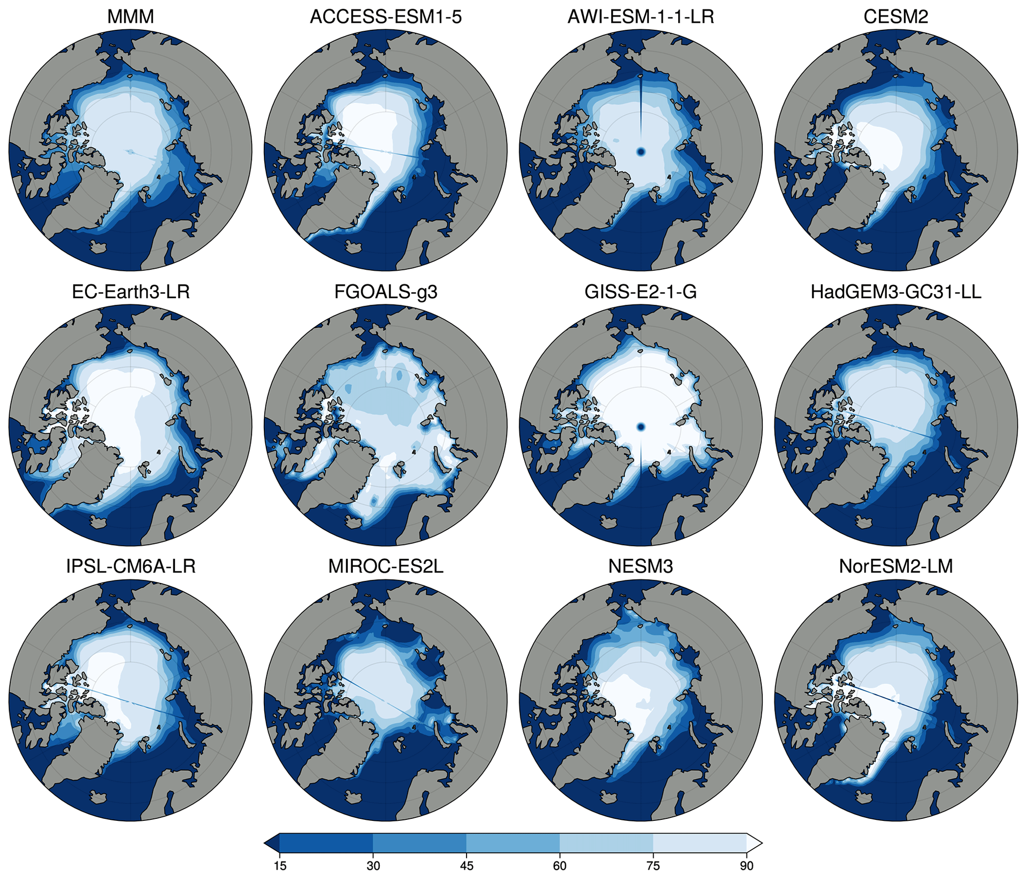
Figure 2 Climatological minimum PI sea ice concentration maps for each model. The first panel represents the multi-model mean (MMM).

For the LIG, the model output is compared against the LIG sea ice synthesis of Kageyama et al. (2021), which include marine cores collected in the Arctic Ocean, Nordic Seas and northern North Atlantic (Fig. 3). These data show that south of 79^∘ N in the Atlantic and Nordic Seas the LIG was seasonally ice free. These southern sea ice records provide quantitative estimates of sea surface parameters based on dinoflagellate cysts (dinocysts). North of 79^∘ N, the sea-ice-related records are more difficult to obtain and interpret. A core at 81.5^∘ N brings evidence of summer probably being seasonally ice-free during the LIG from two indicators: dinocysts and IP25/PIP25. However, an anomalous core close by at the northernmost location of 81.9^∘ N with good chronology shows IP25-based evidence of substantial (>75 %) sea ice concentration all year round. Other northerly cores do not currently have good enough chronological control to confidently date material of LIG age. All models except FGOALS generally tend to match the results from proxies of summertime Arctic sea ice in marine cores with good LIG chronology (Fig. 3), apart from the anomalous northernmost core for which the IP25 evidence suggest perennial sea ice (Kageyama et al., 2021). Stein et al. (2017) suggest that PIP25 records obtained from the central Arctic Ocean cores indicating a perennial sea ice cover have to be interpreted cautiously, given that biomarker concentrations are very low to absent, and thus it is difficult to know how much weight to place on this particular result. Additionally, given Hillaire-Marcel et al. (2017) question the age model of the data from the central Arctic Ocean, these IP25 data need to be interpreted with some caution. This may mean that all the models tend to have similar problems in simulating Arctic sea ice during the LIG or that the LIG IP25 signal in the Arctic indicates something else. What is clear is that a new approach with other Arctic datasets, such as SSAT, may be needed to make progress on the LIG Arctic sea ice question.

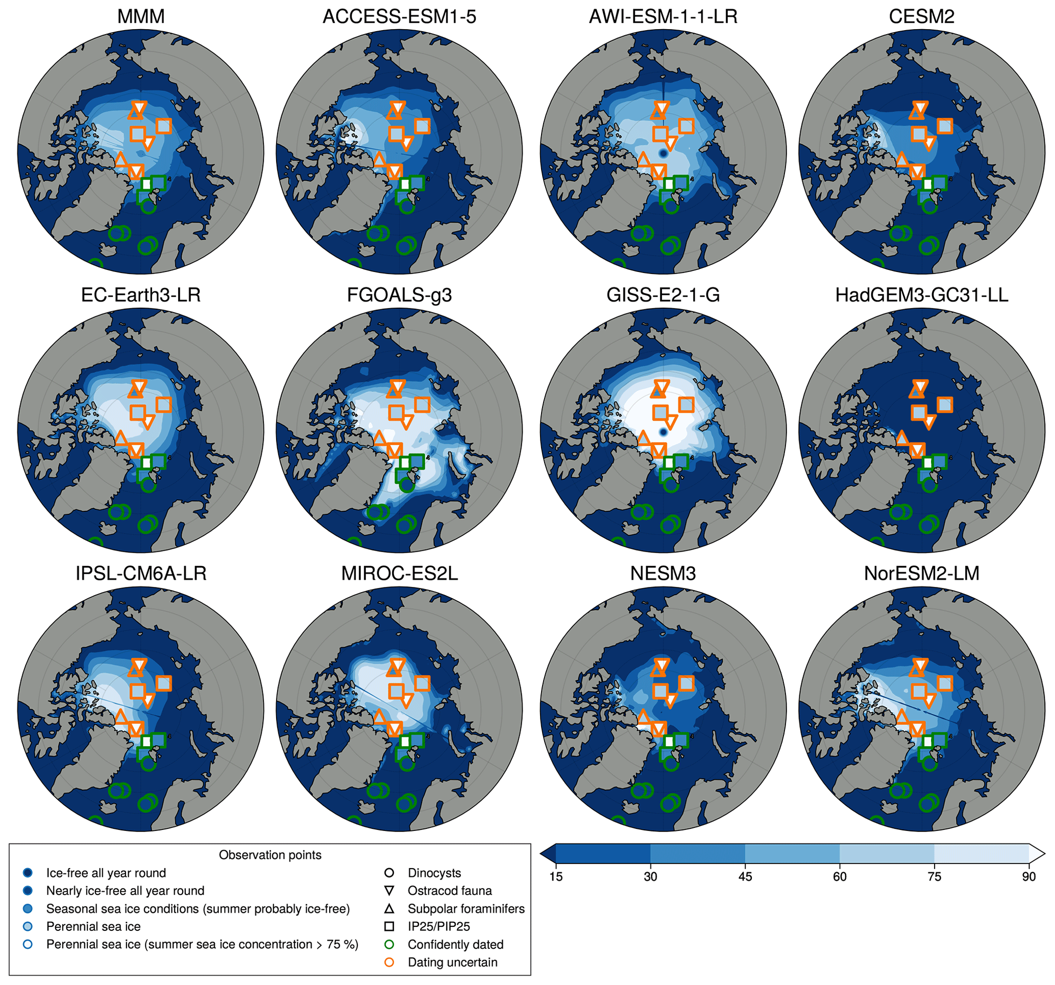
Figure 3 Climatological minimum LIG sea ice concentration maps for each model. Marine core results are from Kageyama et al. (2021): orange outlines indicate that the dating is uncertain; green outlines indicate the data point is from the LIG. The first panel represents the multi-model mean.

For the LIG, there is very little difference between the maximum (wintertime) Arctic SIA and that of the PI period (which is 15–16×10⁶ km² between the PI period and the LIG in most models), but every model shows a reduction in summer sea ice in the LIG compared to the PI period (Table 2). Our model mean LIG summertime Arctic is 2.9×10⁶ km², compared to 6.4×10⁶ km² for the PI period, or a 55 % PI to LIG decrease. There is large inter-model variability for the LIG SIA during the summer (Fig. 4). All models show a larger sea ice area seasonal amplitude for LIG than for PI, and the range of model SIA is larger for the LIG than for the PI period (Fig. A2). The results for individual years show that no model is close to the ice-free threshold in summer during their PI simulation (Fig. 4), but for the LIG summer SIA there are three models that are lower than 1×10⁶ km² for at least one summer during the LIG simulation (Fig. 4). Of these three, HadGEM3 shows a LIG Arctic Ocean free of sea ice in all summers, i.e. its maximum SIE is lower than 1×10⁶ km² in all LIG simulation years. CESM2 and NESM3 show low climatological SIA values (slightly above 2×10⁶ km²) in summer for the LIG simulation, and both have at least 1 year with a SIE minimum that is below 1×10⁶ km², although their average minimum SIE values are just below 3×10⁶ km². Of these low LIG sea ice models, HadGEM3 and CESM2 realistically capture the PI Arctic sea ice seasonal cycle, while NESM3 overestimates winter ice and the amplitude of the seasonal cycle (Cao et al., 2018).

Table 2 The minimum climatological sea ice area for the PI and the LIG, changes, and the associated ΔSSAT anomalies. Percentage reductions are calculated from PI minimum SIA for each model.

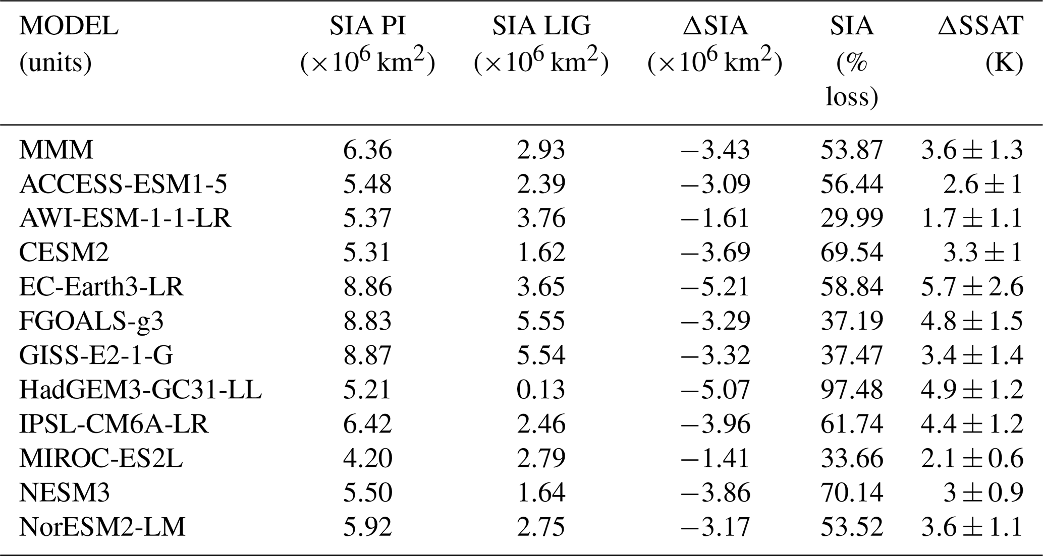
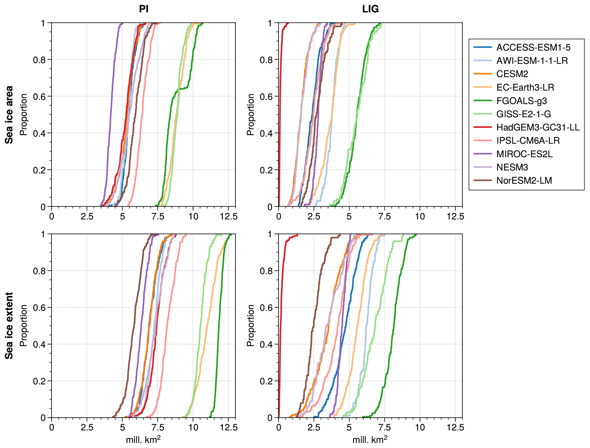
Figure 4 Cumulative distribution of minimum SIA of individual years in LIG and PI simulations, i.e. SIA versus proportion of years that fall below the corresponding SIA value. HadGEM3 has a minimum SIA below 1×10⁶ km² for all years in LIG runs. CESM2 has 6.5 % LIG years with an SIA below 1×10⁶ km², and NESM3 has 8 % LIG years with an SIA below 1×10⁶ km². The lower panels are the same but for SIE.

3.2 Estimating ΔSIA from model skill to simulate ΔSSAT

We first investigate whether there is a relationship between how well models match proxy ΔSSAT and the magnitude of SIA reduction that they simulate for the LIG. A visual comparison of modelled ΔSSAT and proxy estimates for ΔSSAT is also shown in Fig. 5. As described in Sect. 2, two different approaches are used to quantify the skill of the models to simulate ΔSSAT, based on (1) the RMSE of the model–data ΔSSAT at the proxy record locations and (2) the percentage ΔSSAT proxies that the model can correctly match within model and data error. Here the focus is on quantifying model skill across all data records, but for reference the model-versus-proxy ΔSSAT for each location is provided for each model individually in Fig. A3. The RMSE skill estimate and the percentage match estimate provide very similar indications of which models have good skill to reproduce proxy ΔSSAT. The five models with the lowest RMSE also have the highest percentage match, and the two models with the highest RMSE have the lowest percentage match (Fig. 6). Both approaches show that the models with better skill to simulate ΔSSAT have a high absolute ΔSIA. The only outlier is EC-Earth, which has an average skill (sixth best model of the 11) but a high SIA reduction at the LIG. This occurs because the EC-Earth PI simulation has an excessive SIA, more than 3×10⁶ km² compared with present-day estimations; this enables it to have a large ΔSIA value, while likely retaining too much LIG SIA. Quantitatively there is a correlation of $r=-\mathrm{0.65}$ (p=0.03) between the magnitude of ΔSIA and the RMSE, and a correlation with r=0.67 (p=0.02) between the magnitude of ΔSIA and the percentage match of the model (Fig. 6). Given that the SIA reduction from the PI period to the LIG could be dependent on the starting SIA at the PI period, we repeat the analysis for percentage SIA loss from the PI period (rather than absolute SIA loss) and find that is correlates similarly to the model skill to reproduce ΔSSAT (Fig. A4).

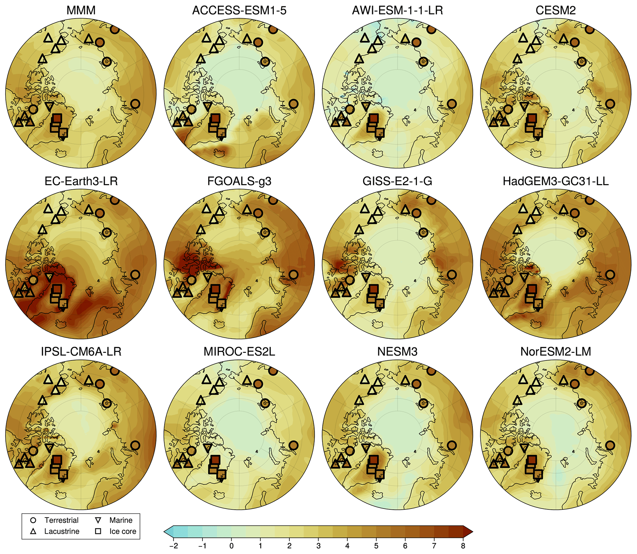
Figure 5 Summertime surface air temperature (SSAT) anomaly (LIG-PI) maps for each model overlain by reconstructed summer temperature anomalies. Proxies are detailed in Table 1 and Guarino et al. (2020b); colours are the same as those used for the underlying model data. The first panel represents the multi-model mean.

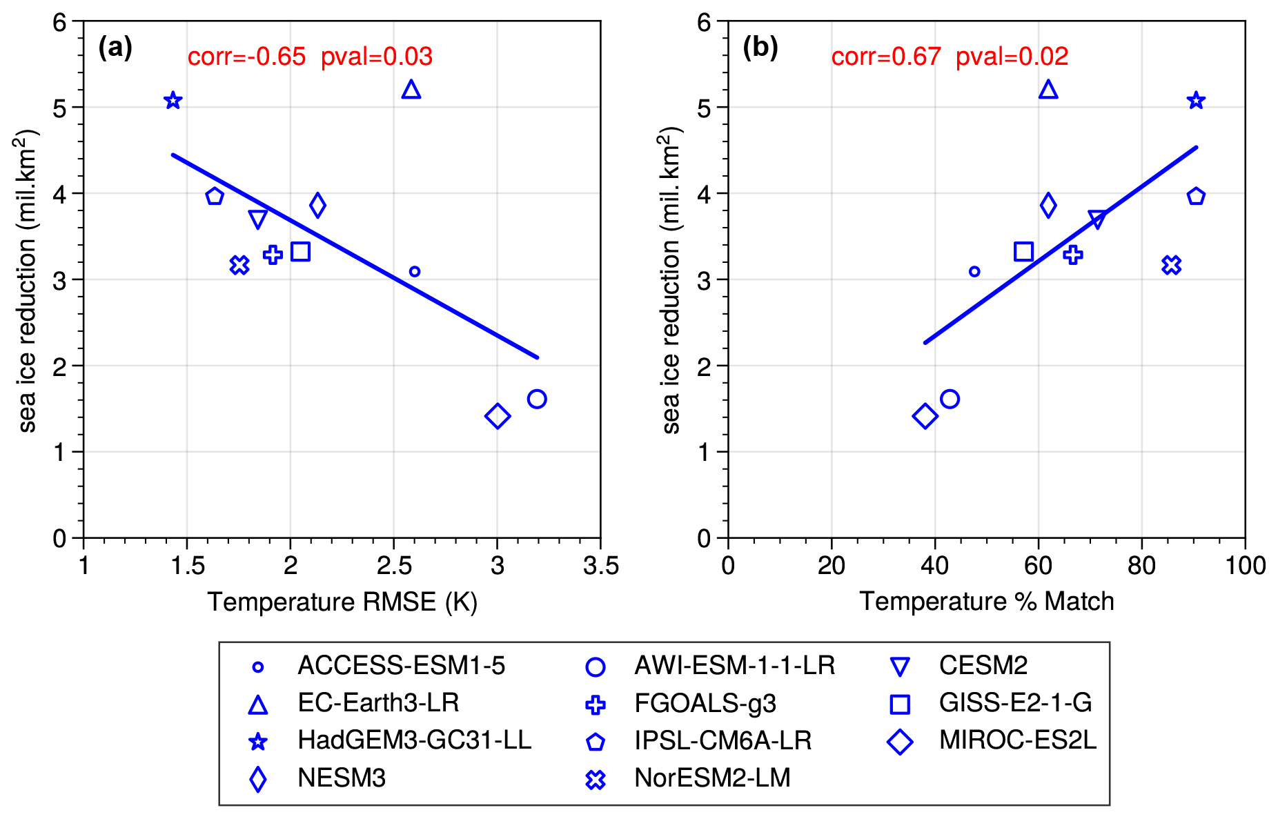
Figure 6 Modelled magnitude of ΔSIA versus model skill to simulate proxy ΔSSAT. (a) The modelled magnitude of ΔSIA is scattered against the RMSE of the modelled ΔSSAT compared to the proxy ΔSSAT for the 21 data locations. (b) The modelled magnitude of ΔSIA scattered against the percentage of ΔSSAT data points that the model can match (see Sect. 2).

In general, where models have a closer match with the ΔSSAT, they have a higher absolute ΔSIA and larger percentage reduction in SIA from the PI period. We thus look at our best-performing models for an indication of true LIG Arctic sea ice reduction. The four models with the best agreement of ΔSSAT to proxies are, in order of skill, HadGEM3, IPSL, NORESM2 and CESM2. The top two best-performing models simulate an average SIA loss of 4.5×10⁶ km² from an average starting PI SIA of 5.8×10⁶ km² to a final LIG SIA of 1.3×10⁶ km², which equates to a percentage SIA loss of 79 %. When also including the third- and fourth-best-performing models in the average results in an average SIA loss of 4.0×10⁶ km² to a final LIG SIA of 1.7×10⁶ km² from an average starting PI SIA of 5.7×10⁶ km², which equates to a percentage SIA loss of 71 %.

The question arises as to why there is a linear relationship between model skill when simulating Arctic ΔSSAT and SIA reduction. One possibility is that the mean proxy ΔSSAT of 4.5 K is higher than what most models produce and that the warmer models are thus closer to the proxies and also more likely to reduce sea ice. In the next section, this question is addressed by investigating whether ΔSIA is closely related to ΔSSAT itself.

3.3 Estimating ΔSIA from the modelled ΔSIA–ΔSSAT relationship and proxy ΔSSAT

Here we investigate whether the models suggest a linear relationship between ΔSSAT and ΔSIA and, if so, exploit that together with proxy ΔSSAT to estimate the most likely (true) value for ΔSIA. We first calculate the mean ΔSSAT in the model at all 21 proxy data locations and compare it to the magnitude of ΔSIA in each model (Fig. 7a). The two are well correlated with r=0.86 (p=0.001), and the regression equation provides a dependence of ΔSIA on ΔSSAT. Using this relation, the reconstructed mean ΔSSAT at the proxy locations (4.5±1.7) points to a SIA reduction of $\mathrm{4.2}\pm \mathrm{1.4}\times {\mathrm{10}}^{\mathrm{6}}$ km² from the PI period. This constitutes about 77 % reduction from the present-day observation of 5.7×10⁶ km², which is also the average SIA for the PI period in the two most skilful models identified in the previous section. Using this value for the PI sea ice suggests that a remaining minimum of 1.3×10⁶ km² of sea ice during the LIG summer. An average LIG minimum of 1.3×10⁶ km² implies that some LIG summers must have been ice free (below 1×10⁶ km² in SIE) but that most summers would have had a small amount of sea ice.

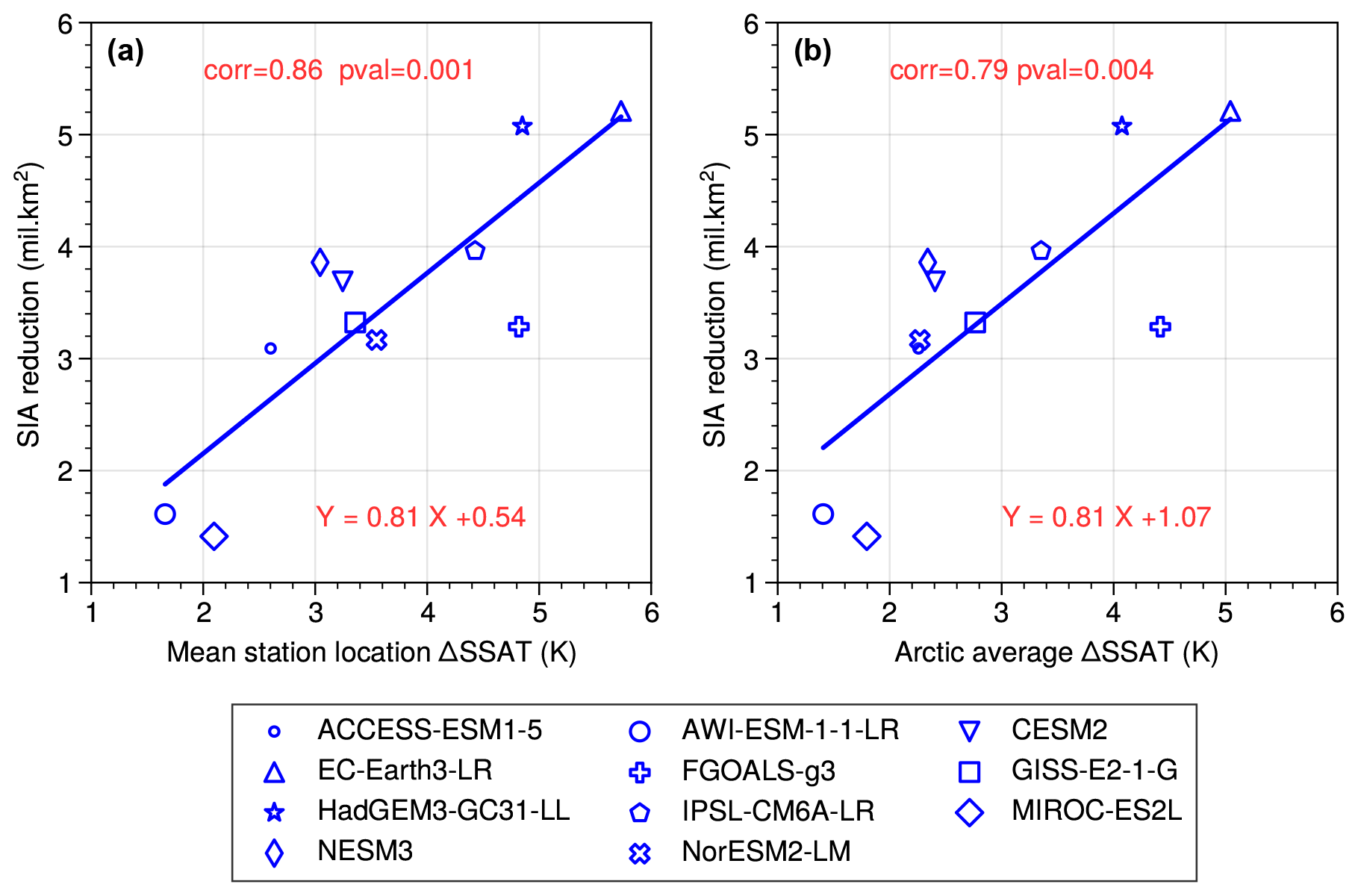
Figure 7 Modelled magnitude of ΔSIA versus modelled ΔSSAT for the Arctic. (a) The modelled ΔSIA is scattered against mean modelled ΔSSAT at the 21 data locations. (b) The modelled ΔSIA is scattered against the mean modelled ΔSSAT averaged over the Arctic north of 60^∘ N.

The ΔSSAT relationship to ΔSIA has so far been computed using the mean ΔSSAT at the locations of the data. To test whether this method would also work for the Arctic in general, the ΔSSAT is next averaged over the whole Arctic north of 60^∘ N and compared with ΔSIA (Fig. 7b). The correlation between ΔSSAT and ΔSIA is a somewhat reduced when calculating ΔSSAT across the whole Arctic, though it is still highly significant (r=0.79, p=0.004). An estimate for proxy-based Arctic-wide ΔSSAT can be derived by applying the close relationship between Arctic ΔSSAT and station ΔSSAT in the models (Fig. 8, r=0.97, p<0.001). Inserting the ΔSSAT averaged over all proxy records of 4.5±1.7 K in the regression equation in Fig. 8 gives an estimate for proxy-based Arctic-wide ΔSSAT of 3.7±1.5 K. Applying the regression equation in Fig. 7b and using this estimate for Arctic-wide ΔSSAT suggests a PI to LIG sea ice reduction of $\mathrm{4.1}\pm \mathrm{1.2}\times {\mathrm{10}}^{\mathrm{6}}$ km², which is very similar to the estimate derived from the station data alone (of $\mathrm{4.2}\pm \mathrm{1.4}\times {\mathrm{10}}^{\mathrm{6}}$ km²).

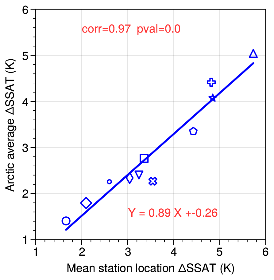
Figure 8 Modelled Arctic-wide ΔSSAT versus modelled mean ΔSSAT at the data locations for the 11 models. The markers for each model are the same as in Fig. 7.

4 Discussion and conclusions

As discussed in the Introduction, neither proxies nor modelling results alone allow currently for a convincing estimate of the Arctic sea ice reduction at the LIG. Here we apply a joint approach to make progress. We deduce how much sea ice was reduced during the LIG, using 11 of the most recent CMIP6-PMIP4 LIG model simulations and proxy observations of summer air temperature changes. The reduction in sea ice from the PI period to the LIG in the models range from 30 % to 96 % with an average of 55 %. No model is close to the ice-free threshold of maximum SIE lower than 1×10⁶ km² for any model year summer during their PI simulation. During the LIG, the HadGEM3 model is the only one that has an Arctic Ocean free of sea ice in all summers, although CESM2 and NESM3 show SIA values of around 2×10⁶ km² associated with intermittently ice-free conditions. We found that larger LIG SIA reduction from the PI period is related to greater SSAT warming, the two being correlated with r=0.86 across the models. In particular, 8 out of 11 models are able to match, within uncertainty, the average PI to LIG summertime Arctic warming of 4.5±1.7 K as recorded by surface temperature proxies. This magnitude of warming was difficult to reach with previous generations of LIG models. Among the models, two of them capture the magnitude of the observed dSSAT in more than 60 % of the total proxy locations. These models simulate an average LIG sea ice area of 1.3×10⁶ km², which is a 4.5×10⁶ km² (or 79 %) reduction from their PI values.

We find that the good match between the (ice-free) HadGEM3 and the Guarino et al. (2020b) summer Arctic temperature dataset is not unique. However, we find that it is not random either and that there is a correlation between model skill to match the ΔSSAT and the reduction in SIA from the PI period to the LIG (both when using an RMSE skill test and when using a best-match skill test). The two most skilful models simulate an average LIG sea ice area of 1.3×10⁶ km², which is a 4.5×10⁶ km² or 79 % reduction from their PI values. While we cannot assume all model error ΔSSAT is attributable to ΔSIA, it is reasonable to assume that the better-performing models for ΔSSAT are also better at simulating ΔSIA because of the close relationship between warming and sea ice loss.

Some of the proxies are more difficult for the models to simulate (Figs. 9 and A3). In particular, it appears that the Greenland ice core SSAT value from NEEM of +8^∘ (proxy record 21 in Table 1 and Fig. 9) is higher than any model simulates; though with a ±4 K uncertainty it is nevertheless matched by some models. Terrestrial proxies three and six, with SSAT values of +6.4 K, are also only rarely matched. Further work on the observational side would be useful. These LIG SSAT proxy reconstructions were used in the IPCC (2013) report and by Guarino et al. (2020b) and were previously published by IPCC (2013), CAPE members (2006), Kaspar et al. (2005), and Capron et al. (2017). Thus, this dataset should ideally be improved. One start point for this would be adding uncertainties to the (nine) sites that do not currently have these numbers.

Figure 9 Proxy ΔSSAT (violet dots and uncertainty bars) and simulated ΔSSAT for all models (coloured dots) for each proxy record location (rows). Grey boxes extend from the 25th to the 75th percentile of each location's distribution of simulated values, and the vertical lines represent the median.

The correlation between model skill to simulate ΔSSAT and the magnitude of ΔSIA is convincing (r=0.66 and p=0.003 on average for the two skill tests). However, the two quantities are not straightforward to relate through a dynamical process. On the other hand, it is well known that there is a positive feedback between Arctic temperature and Arctic sea ice, with warmer temperatures more likely to melt sea ice, and less sea ice producing a smaller albedo to incoming solar radiation and thus less cooling from solar reflection. Figure A6 shows the relationship between summer surface air temperature anomalies versus September sea ice area from the observational estimates for the period from 1979–2020. At present, the relationship between minimum SIA and summer SAT is a 1.32×10⁶ km² decrease per 1 K temperature rise. This dynamic relationship is also evident in LIG simulations, with a strong correlation of r=0.86 between the magnitude of ΔSIA and ΔSSAT across all the models, and the inter-model relationship suggests a sea ice decrease of 1.9×10⁶ km² per 1 K temperature rise (from the regression equation in Fig. 7b). The reconstructed ΔSSAT from proxies, of 4.5±1.7 K, is larger than most models simulate, and thus the models that match the ΔSSAT most closely would be the models with a larger ΔSSAT than average and a larger ΔSIA. The only model that has a large SIA reduction and not a good skill to match SSAT is EC-Earth, which features a PI simulation with far too much sea ice that allows an excessive LIG to PI Arctic warming. An additional result of our study is that the mean ΔSSAT at the proxy locations is strongly correlated to Arctic-wide ΔSSAT north of 60^∘ N in the models (r=0.97). Applying the regression relation between the two implies that the mean ΔSSAT at the proxy locations, 4.5±1.7 K, is equivalent to an Arctic-wide warming at the LIG of 3.7±1.5 K. This is thus a more representative value for the Arctic warming at the LIG than using the simpler proxy-location average.

The strong linear correlation between the magnitude of ΔSIA and ΔSSAT is applied to the proxy-reconstructed ΔSSAT to give an estimate of the reduction in SIA from the PI period to LIG of $\mathrm{4.2}\pm \mathrm{1.4}\times {\mathrm{10}}^{\mathrm{6}}$ km², similar to that derived from our “best skill” approach. A similar value of $\mathrm{4.1}\pm \mathrm{1.2}\times {\mathrm{10}}^{\mathrm{6}}$ km² is obtained when extrapolating the method to Arctic-wide ΔSSAT north of 60^∘ N. The models and data have uncertainties, and the regressions applied are not between perfectly correlated quantities. However, it is clear from both applied methods (each with two variants) that proxy-reconstructed ΔSSAT, in combination with the model output, implies a larger sea ice reduction than the climatological multi-model mean of 55 %. It suggests a LIG SIA of $\sim \mathrm{1.5}\times {\mathrm{10}}^{\mathrm{6}}$ km², which is consistent with intermittently ice-free summers – but with (low-ice-area) ice-present summers likely exceeding the number of ice-free years.

While we have focussed here on the Arctic SIA response to LIG insolation forcing, Kageyama et al. (2021) found that the models that respond strongly to LIG insolation forcing also respond strongly to CO₂ forcing. Indeed the models with the weakest response for the LIG had the weakest response to the CO₂ forcing. This suggests that our assessment here of model skill against Arctic SIA and SSAT change can also help to some extent in ascertaining the models that have a better Arctic SIA and SSAT response to CO₂ forcing. Overall, the results presented in this study suggest that (i) the fully ice-free HadGEM3 model is somewhat too sensitive to forcing as it loses summer sea ice too readily during the LIG, and (ii) most other PMIP4 models are insufficiently sensitive as these models do not lose enough sea ice.

Appendix A: Inter-model differences in LIG sea ice simulation

Sea ice formation and melting can be affected by a large number of factors inherent to the atmosphere and the ocean dynamics, alongside the representation of sea ice itself within the model (i.e. the type of sea ice scheme used). In coupled models it can therefore be difficult to identify the causes of this coupled behaviour (Kageyama et al., 2021; Sicard et al., 2022). Nevertheless, Kageyama et al. (2021; Sect. 4), alongside Diamond et al. (2021), address the question of what drives model differences in summertime LIG sea ice. Their points can be summarized as follows.

1. All PMIP4-LIG simulations show a major loss of summertime Arctic sea ice between the PI period and LIG.

2. Across all models, there is an increased downward shortwave flux in spring due to the imposed insolation forcing and a decreased upward shortwave flux in summer, related to the decrease in the albedo due to the smaller sea ice cover. Differences between the model results are due to a difference in phasing of the downward and upward shortwave radiation anomalies.

3. The sea ice albedo feedback is most effective in HadGEM3. It is also the only model in which the anomalies in downward and upward shortwave radiation are exactly in phase.

4. The CESM2 and HadGEM3 models (which both simulate significant sea ice loss) exhibit an Atlantic meridional overturning circulation (AMOC) that is almost unchanged between PI and LIG, while in the IPSLCM6 model (with moderate sea ice loss) the AMOC weakens. This implies that a reduced northward oceanic heat transport could reduce sea ice loss in the central Arctic in some models.

5. The two models (HadGEM3 and CESM2) that had the lowest sea ice loss contain explicit melt pond schemes, which impact the albedo feedback in these models. Diamond et al. (2021) show that the summer ice melt in HadGEM3 is predominantly driven by thermodynamic processes and that those thermodynamic processes are significantly impacted by melt ponds.

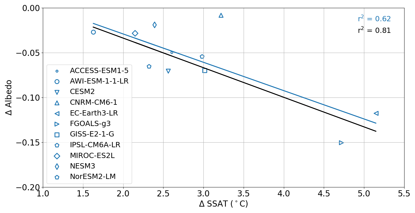
Figure A1 LIG–PI change in albedo over Arctic sea ice as a function of LIG–PI change in SSAT (^∘C) over the ice. The r² values and the linear fit lines are for the models including CNRM (blue) and excluding CNRM (black). The CNRM model (upward-pointing triangle) is an outlier that influences the strength rather than the nature of the correlation.

Figure A2 Sea ice area climatological seasonal cycle for each model.

Figure A3 Modelled ΔSSAT versus proxy ΔSSAT. The scatter points show model data versus reconstructions for each proxy location. Error bars represent 1 standard deviation on either side of the proxy estimate. The correlation coefficients between X and Y, RMSE, and percentage matches with proxy data for each model are indicated in each panel.

Figure A4 Modelled percentage sea ice area reduction from the LIG to the PI period versus model skill to simulate proxy ΔSSAT. (a) The modelled percentage SIA reduction is scattered against the RMSE of the modelled ΔSSAT compared to the proxy ΔSSAT for the 21 data locations. (b) The modelled percentage SIA reduction scattered against the percentage of ΔSSAT data points that the model can match (see Sect. 2).

Figure A5 Scatterplot for climatological ΔSSAT at each proxy location versus climatological ΔSSAT averaged north of 60^∘ N in each model.

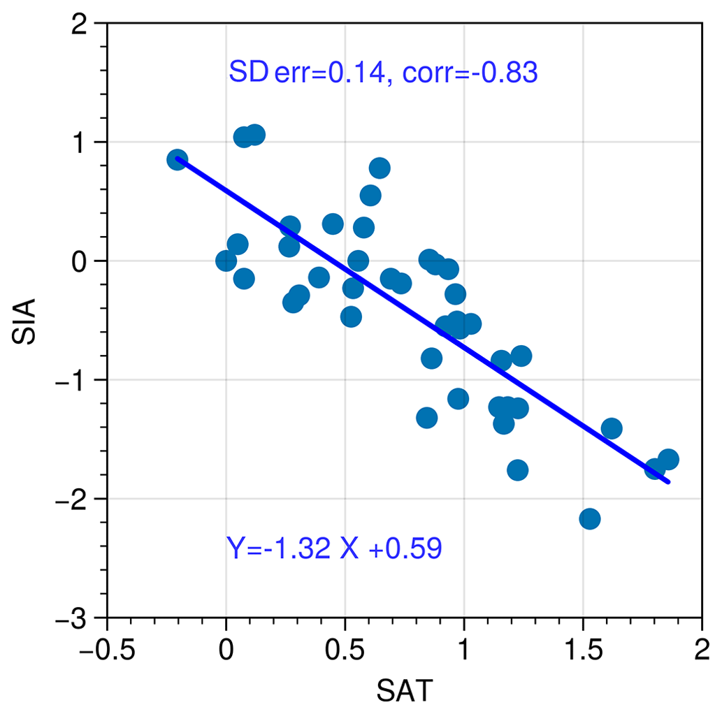
Figure A6 Scatterplot of SAT versus SIA for current period. June–July– August (JJA) surface air temperature versus Northern Hemisphere September sea ice area for each year from 1979 to 2020. Anomalies computed from year 1979 values. SIA is from NSIDC (https://nsidc.org/data/g02135/versions/3, last access: 28 October 2022), and air temperature (area averaged north of 60^∘ N) is from ERA5 reanalysis (Hersbach et al., 2020).