Reconstructing atmospheric H₂ over the past century from bi-polar firn air records

Historical atmospheric H₂ levels were reconstructed using firn air measurements from two sites in Greenland (NEEM and Summit) and two sites in Antarctica (South Pole and Megadunes). A joint reconstruction based on the two Antarctic sites yields H₂ levels monotonically increasing from about 330 ppb in 1900 to 550 ppb in the late 1990s, leveling off thereafter. These results are similar to individual reconstructions published previously (Patterson et al., 2020, 2021). Interpretation of the Greenland firn air measurements is complicated by challenges in modeling enrichment induced by pore close-off at these sites. We used observations of neon enrichment at NEEM and Summit to tune the parameterization of enrichment induced by pore close-off in our firn air model. The joint reconstruction from the Greenland data shows H₂ levels rising 30 % between 1950 and the late 1980s, reaching a maximum of 530 ppb. After 1990, reconstructed atmospheric H₂ levels over Greenland are roughly constant, with a small decline of 3 % over the next 25 years. The reconstruction shows good agreement with the available flask measurements of H₂ at high northern latitudes.

1 Introduction

Molecular hydrogen (H₂) is the second-most abundant reduced gas in Earth's atmosphere after methane. Atmospheric H₂ levels are linked to Earth's radiative budget, air quality, and the atmospheric oxidative capacity (e.g., Ehhalt and Rohrer, 2009; Novelli et al., 1999; Paulot et al., 2021). As H₂ becomes a more important component of the energy sector, anthropogenic emissions of H₂ are expected to rise substantially (Derwent et al., 2020; Prather, 2003; Wang et al., 2013a, b). Projecting the atmospheric response to increased anthropogenic emissions in a changing climate requires a comprehensive understanding of the biogeochemical cycle of H₂. Studying past changes in atmospheric H₂ can inform predictions of the effects of future perturbations by providing insight into the relationship between atmospheric H₂, human activities, and climate.

The globally averaged mixing ratio of H₂ in the present-day atmosphere is roughly 530 nmol mol⁻¹ (ppb; Pétron et al., 2023). Major sources of atmospheric H₂include photochemical production from the oxidation of methane and non-methane hydrocarbons (NMHCs) as well as direct emissions from fossil fuel combustion and biomass burning. Direct emission as a by-product of N₂ fixation is a minor source of atmospheric H₂. The major sink of atmospheric H₂ is consumption by soil microbes, accounting for about 70 % of total losses, and the remainder of the losses are to oxidation by the OH radical. Based on the atmospheric burden and estimates of the microbial and OH sinks, the lifetime of H₂ is estimated at 2 years (Novelli et al., 1999; Pieterse et al., 2011, 2013; Paulot et al., 2021).

Increasing atmospheric H₂ could influence the climate system in several ways. The reaction of H₂ with OH represents a loss for OH and therefore increases the atmospheric methane lifetime and associated radiative forcing. This reaction leads to the production of HO₂, which can influence tropospheric ozone levels. In the stratosphere, the reaction of H₂ with OH leads to the production of water vapor. Increased stratospheric water vapor cools the stratosphere and warms the troposphere (Solomon et al., 2010). Paulot et al. (2021) estimated the effective radiative forcing of atmospheric H₂ at 0.13 mW m⁻² ppb⁻¹ due to its effects on the methane lifetime and stratospheric water vapor content.

Systematic measurements of atmospheric H₂ levels began in the late 1980s (Khalil and Rasmussen, 1990). The NOAA Global Monitoring Laboratory (NOAA/GML), CSIRO GASLAB (CSIRO), and the Advanced Global Atmospheric Gases Experiment (AGAGE) started to monitor atmospheric H₂ levels at several sites around the world in the early 1990s (Novelli et al., 1999; Novelli, 2006; Prinn et al., 2019; Langenfelds et al., 2002; Pétron et al., 2023). Integration of records produced by the different groups has been complicated by calibration issues. Earlier use of different scales was addressed by implementation of the internationally accepted MPI09 scale established by the Max Planck Institute for Biogeochemistry (MPI; Jordan and Steinberg, 2011). Measurements from CSIRO and AGAGE have been transferred to the MPI09 scale. Additionally, NOAA/GML measurements from 2009 onward were recently revised to the MPI09 scale (Pétron et al., 2023). Broadly, the instrumental record shows northern hemispheric H₂ levels rising during the late 1980s to a maximum in 1990 and decreasing until 1993. There is no discernible trend in Northern Hemisphere H₂ levels from 1993–2010 (Fig. 7). The Southern Hemisphere instrumental record shows H₂ levels rising until 1999, then plateauing for the next 10–15 years.

Longer-term changes in atmospheric H₂ levels during the 20th century have been reconstructed using polar firn air from Antarctica (South Pole, Megadunes) and Greenland (NEEM; Petrenko et al., 2013; Patterson et al., 2020, 2021). Firn is the compacted snow layer that forms the upper 40–120 m of ice sheets, and its interconnected porosity contains an atmospheric archive (referred to as “firn air”) that can extend up to ∼100 years back in time. For a comprehensive introduction to firn and firn air we refer the interested reader to Buizert (2013). The Antarctic reconstructions show that H₂ levels increased by 60 % over the 20th century, consistent with increasing anthropogenic emissions and photochemical production from methane (Patterson et al., 2020). The Greenland reconstruction shows an increase in atmospheric H₂ levels during the 1960s to a peak in the late 1980s or early 1990s, followed by a small decline from 1990–2009 (Petrenko et al., 2013). This recent decline is inconsistent with Northern Hemisphere modern flask measurements that show roughly constant H₂ levels after the mid-1990s (Novelli, 2006; Prinn et al., 2019). Petrenko et al. (2013) noted that the firn air model used for that reconstruction did not include pore close-off fractionation, a process that enriches H₂ in the lock-in zone where vertical diffusion of trace gases effectively goes to zero. Patterson et al. (2021) suggested that the inferred peak could be an artifact of ignoring this process.

In this work, we reassess historical Northern Hemisphere atmospheric H₂ levels over the 20th century using firn air from NEEM and an additional Greenland site with previously unpublished H₂ measurements (Summit). Additionally, we reanalyze the Antarctic firn air data using a different inversion technique described in Sect. 3.3. Reliable bi-polar records are useful for constraining changes to H₂ cycling because the two hemispheres differ in their sensitivity to changes in the soil sink and anthropogenic emissions. Understanding past variability in the soil sink is particularly important because the response of the soil sink to future changes in climate is the largest source of uncertainty in projecting the radiative consequences of increasing anthropogenic H₂ emissions (Warwick et al., 2022).

2 H₂ measurements in Greenland firn air

2.1 Firn air sampling

The sampling methods used in the Summit and NEEM campaigns were similar to techniques from previous published firn air studies (e.g., Battle et al., 1996; Severinghaus et al., 2001; Severinghaus and Battle, 2006). Briefly, a borehole was drilled into the firn, pausing the drilling at each desired sampling depth. The borehole was sealed above each sampling depth with an inflatable rubber packer to prevent contamination from the modern atmosphere. Synflex 1300 (formerly known as “Decabon”) tubing for both waste air and sample air extends from below the packer to the surface. The waste air intake was positioned directly below the rubber packer. The waste air intake was separated from the sample air intake by a stainless-steel plate (baffle) with a diameter slightly less than the borehole. Air was pumped from the waste air intake 2–5 times faster than from the sample air intake to ensure that no air that had been in contact with the rubber packer was sampled. Sampled air was dried using Mg(ClO₄)₂ and stored in 2.5 L glass flasks. More detailed information regarding the sampling at each site may be found in the references listed in Table 1.

Table 1 Site characteristics and data references for the three Greenland firn air sampling campaigns.

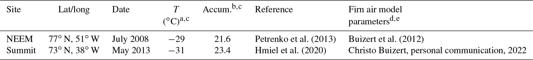
^a Mean annual surface temperature. ^b Average modern accumulation (cm ice equivalent per year). ^c Temperature and accumulation for NEEM are from Buizert et al. (2012). Temperature and accumulation for Summit were supplied by Christo Buizert (personal communication, 2022). ^d Modeling parameters include density profile and the lock-in depth (Sect. 3.1). ^e Partitioning between closed and open porosity is described in Sect. 3.2.

2.2 Firn air measurements and calibration

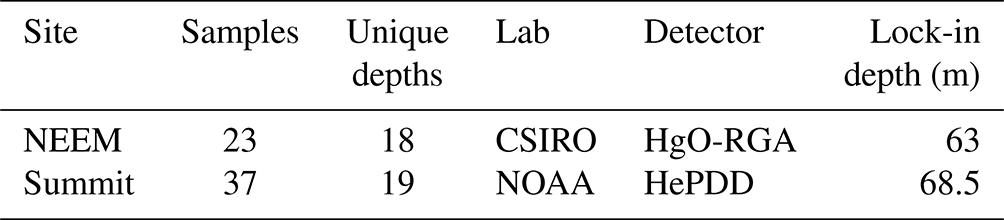
The Summit firn air measurements were made by NOAA/GML using a helium pulsed-discharge detector with a linear response (HePDD; Novelli et al., 2009). The Summit measurements have been formally revised from the NOAA96 to the MPI09 calibration scale using a long-term matched flask intercomparison project, which began in 1992 (Pétron et al., 2023). Firn air samples from NEEM were analyzed for H₂ at CSIRO using gas chromatography coupled to a mercuric oxide reductive gas analyzer (HgO-RGA). These measurements were calibrated using standards between 340 and 1000 ppb. The CSIRO measurements have been formally revised from the CSIRO94 to the MPI09 calibration scale (Jordan and Steinberg, 2011). CSIRO estimates the analytical uncertainty to be ±0.2 %. However, there are other sources of uncertainty in the true H₂ content in the firn air. For example, tests conducted during the NEEM campaign demonstrated a small procedural blank (4–6 ppb). No such tests were conducted at Summit. To account for the possibility of such blanks, we assign an overall uncertainty of ±2 % to the data from NEEM and Summit. The Antarctic firn air measurements have been described previously (Patterson et al., 2020, 2021).

The firn air H₂ measurements from all sites were corrected for gravitational fractionation (Eq. 2; Sect. 3.1), and duplicate measurements at the same depth were averaged to generate the finalized depth profiles (Fig. 4b, c; Fig. 5b, c; Fig. 6b, c). Lock-in depths for the sites are given in Table 2. The H₂ depth profiles at the Greenland sites display strong gradients above lock-in that reflect the fast free-air diffusivity of H₂ and intense seasonality of atmospheric H₂ in the Northern Hemisphere. The H₂ gradient observed in the upper firn at NEEM is different than the gradient at Summit because NEEM was sampled in July, while the other site was sampled in May. The depth profiles from NEEM and Summit both display sharp maxima of 530 and 560 ppb, respectively, in the lock-in zone. The NEEM measurements also show a sharp decrease to 490 ppb at the bottom of lock-in. At Summit, the decrease towards the bottom of lock-in is less dramatic than at NEEM because only one sample depth is deeper than the observed maximum. The qualitative differences in the depth profiles reflect changes in surface air H₂ levels over the period of the firn air sampling (2008–2013) and the different physical characteristics of the sites. For example, the firn air at the bottom of the lock-in zone at Summit is younger than at NEEM because Summit was sampled several years later and has a thinner lock-in zone (Table 1).

Table 2 Summary of firn air H₂ measurements from NEEM and Summit.

3 Firn air modeling and inversions

3.1 Firn air model

The UCI_2 firn air model is a one-dimensional finite-difference advective–diffusive model that is used to simulate the evolution of trace gas levels in firn air. The UCI_2 model has been used to successfully analyze H₂ levels in firn air at the two Antarctic sites, including the effects of pore close-off fractionation (see below; Patterson et al., 2020, 2021). The default model parameterizations do not adequately capture the effects of pore close-off fractionation at the Greenland sites, and additional tuning is required as described in Sect. 3.2.

The UCI_2 model is largely based on Severinghaus et al. (2010). The model domain is divided into an upper “diffusive zone” and lower “lock-in zone.” In the diffusive zone, vertical gas transport occurs via wind-driven mixing in the shallowest ∼5 m and via molecular diffusion throughout. Diffusive mixing decreases with depth due to the increasing tortuosity of the firn. In the lock-in zone, vertical molecular diffusion ceases due to the presence of impermeable ice layers. Gas transport in the lock-in zone occurs primarily due to advection with a small non-fractionating mixing term. The model uses a forward Euler integration scheme and a time step of 324 s. There are two important differences between the Severinghaus et al. (2010) model and the UCI_2 model: (1) thermal diffusion is neglected, as it is unimportant for H₂, and (2) our model parameterizes pore close-off fractionation differently than the Severinghaus model (Sect. 3.2). The UCI_2 model tracks the air content and composition in both open pores and closed bubbles as a function of time and depth. The model code is written and executed in MATLAB R2022a (Mathworks Inc.).

The site-specific bulk density profile (ρ_firn: kg m⁻³) is calculated from an empirical fit to density measurements of the firn core. Total porosity (s_total; dimensionless) is estimated from the density profile:

$$\begin{array}{}\text{(1)}& s_{\mathrm{total}}=\mathrm{1}-{\displaystyle \frac{{\mathit{\rho }}_{\mathrm{firn}}}{{\mathit{\rho }}_{\mathrm{ice}}}},\end{array}$$

where ρ_ice (kg m⁻³) is the temperature-dependent density of ice from Bader (1964). Accumulation rate, temperature, and the depth of the lock-in zone onset are site-specific parameters. Partitioning between closed and open porosity in the model is described in Sect. 3.2.

Model grid spacing is 0.5 m in the diffusive zone. Gas transport is dominated by wind-driven mixing in the upper part of the diffusive zone and by molecular diffusion in the lower part of the diffusive zone. To simulate non-fractionating wind-driven mixing, a depth-dependent eddy diffusivity term is added to the one-dimensional firn air transport equation (Schwander et al., 1993; Severinghaus et al., 2010; Trudinger et al., 1997). Additionally, we neglect the typical gravitational term and instead empirically correct the firn air measurements using the δ¹⁵N of N₂ depth profile. The correction is calculated from the δ¹⁵N data for each borehole according to Eq. (2):

$$\begin{array}{}\text{(2)}& {\mathrm{Corr}}_{\mathrm{grav}}={\displaystyle \frac{{\mathit{\delta }}^{\mathrm{15}}\mathrm{N}}{\mathrm{1000}}}\cdot {\displaystyle \frac{\exp \left(g\cdot z\cdot \frac{\mathrm{\Delta }{m}_{\mathrm{g}}}{RT}\right)-\mathrm{1}}{\exp \left(g\cdot z\cdot \frac{\mathrm{\Delta }{m}_{{}^{\mathrm{15}}\mathrm{N}}}{RT}\right)-\mathrm{1}}},\end{array}$$

where Corr_grav is the depth-dependent fractional correction for the gas of interest, δ¹⁵N is the measured isotopic composition of N₂ (‰) each depth, g is the gravitational acceleration constant (9.8 m s⁻²), z is depth (m), R is the ideal gas constant (8.314 J mol⁻¹ K⁻¹), T is the annual average temperature at the site, Δm_g is the difference in molar mass (in kg) between the gas of interest and air, and $\mathrm{\Delta }{m}_{{}^{\mathrm{15}}\mathrm{N}}$ is the difference in molar mass between ²⁸N₂ and ²⁹N₂ (0.001 kg). This correction neglects the thermal fractionation of δ¹⁵N. Thermal fractionation is only important in the upper ∼20 m of the firn, and these shallow measurements are excluded from the reconstructions due to seasonality in atmospheric H₂ levels (Severinghaus et al., 2001; Sect. 3.2).

Equation (3) governs the evolution of the concentration of the gas of interest in the open pores in the diffusive zone (Severinghaus et al., 2010):

$$\begin{array}{}\text{(3)}& \begin{array}{rl}{s}_{\mathrm{o}}{\displaystyle \frac{\partial C}{\partial t}}& ={\displaystyle \frac{\partial }{\partial z}}\left({\displaystyle \frac{\partial C}{\partial z}}\cdot \left[s_{\mathrm{o}}{D}_{\mathrm{mol}}(z,T,P)+s_{\mathrm{o}}{D}_{\mathrm{eddy}}\left(z\right)\right]\right)\\ & -s_{\mathrm{o}}w{\displaystyle \frac{\partial C}{\partial z}},\end{array}\end{array}$$

where s_o is the open porosity; C is concentration of the gas of interest (mol m⁻³); D_mol is the gas-, depth-, temperature-, and pressure-dependent molecular diffusivity constant (m² s⁻¹); D_eddy is the depth-dependent eddy diffusivity (m² s⁻¹); and w is the downward velocity of the firn column (m s⁻¹). D_mol and D_eddy profiles for NEEM and Summit are tuned using a suite of measured gases with well-constrained atmospheric histories including CO₂, CH₄, CH₃CCl₃, and SF₆. The diffusivity profiles were validated by forcing the model with the established atmospheric histories for the previously mentioned trace gases and comparing the model output to the measurements (Fig. S5). During the tuning process, the ratio between the effective molecular diffusivities of each trace gas at each depth is forced to maintain the ratio of their free-air diffusivities (e.g., at each depth D_mol for CH₄ is 1.4 times that of D_mol for CO₂). After tuning D_mol is then scaled using the ratio of the free-air diffusivity of CO₂ to the diffusivity of H₂ or another trace gas of interest. Temperature- and pressure-dependent free-air diffusivities are calculated using Fuller et al. (1966) as described by Reid et al. (1987; Chap. 11).

Model grid spacing in the lock-in zone is one annual layer. There is no molecular diffusivity in the lock-in zone and gas transport occurs via downward advection of annual layers once per year. Small values of non-fractionating “eddy diffusivity” are prescribed to account for dispersive mixing caused by barometric pressure fluctuations (Buizert and Severinghaus, 2016). Model parameterizations for vertical mixing in the lock-in zone are validated by forcing the model with best-estimate Greenland atmospheric histories for various trace gases with well-constrained atmospheric histories (Buizert et al., 2012).

3.2 Pore close-off fractionation

In addition to wind-driven mixing, diffusion, and advection, pore close-off fractionation is parameterized in the firn air model. As closed pores (bubbles) are advected downward in the firn, internal pressure increases, creating a partial pressure gradient which drives a net diffusive flux of highly mobile trace gases out of the bubbles, through the ice lattice, and into the open pores. The open pores are therefore enriched in these gases. This phenomenon affects gases with kinetic diameter (KD) < 3.6 Å such as Ne and He due to their high diffusivity in ice (Severinghaus and Battle, 2006).

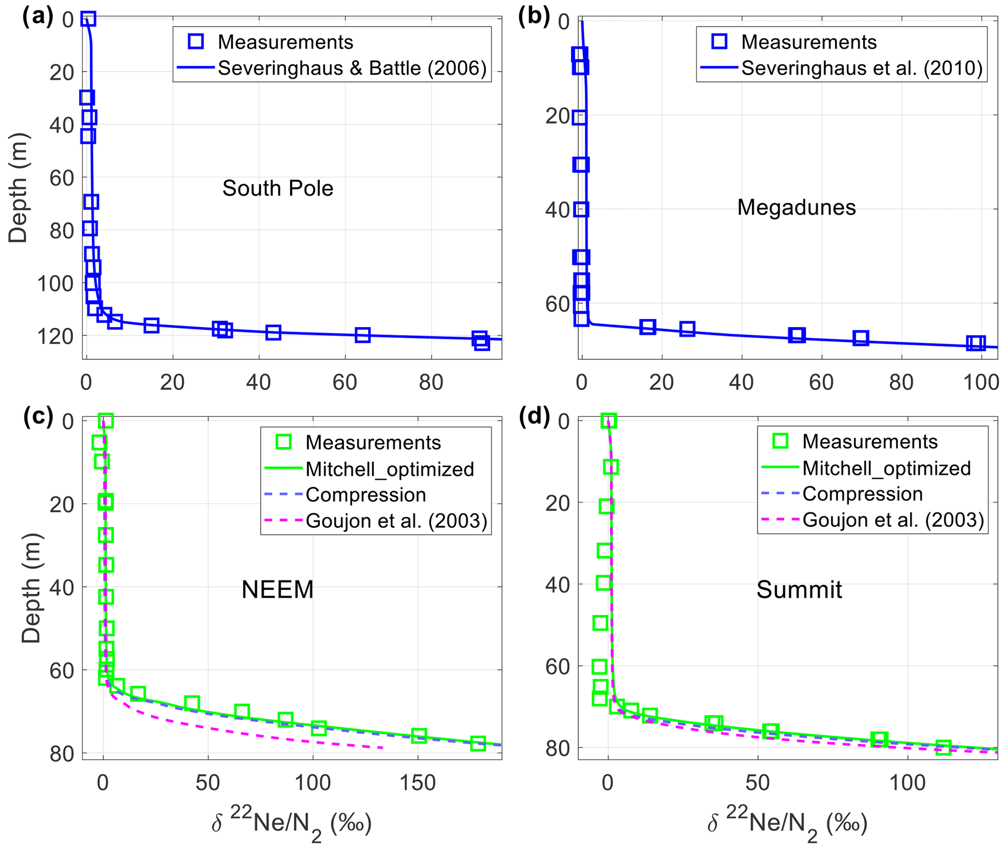
Figure 1 Measured and modeled depth profiles of ²²Ne in the firn air at South Pole (a), Megadunes (b), NEEM (c), and Summit (d). The partitioning between closed and open porosity in the firn air model is from Severinghaus and Battle (2006) and Severinghaus et al. (2010) for South Pole and Megadunes, respectively, as in Patterson et al. (2020, 2021). For NEEM and Summit, several model configurations with different porosity partitioning parameterizations are plotted: Mitchell_optimized (green lines), Compression (dashed purple lines), and Goujon et al. (2003; dashed magenta lines). See text for a description of each configuration.

Given its small molecular diameter (KD = 2.89 Å) pore close-off fractionation must affect H₂ in a manner similar to neon (Patterson et al., 2020; Petrenko et al., 2013; Severinghaus and Battle, 2006). Recent laboratory measurements indicate that the permeability of H₂ in ice is sufficiently fast to equalize the partial pressure of H₂ in the open porosity and closed bubbles (Patterson and Saltzman, 2021). Therefore, in the model, it is assumed that the partial pressure of H₂ is in equilibrium between the closed bubbles and open pores in each layer as described by Eqs. (4)–(6).

$$\begin{array}{}\text{(4)}& P_n=\left(P_{\mathrm{bubble}}{x}_{n\left(\mathrm{bubble}\right)}{s}_{\mathrm{c}}+P_{\mathrm{ambient}}{x}_{n\left(\mathrm{firn}\right)}{s}_{\mathrm{o}}\right)/s_{\mathrm{total}}\end{array}$$

$$\begin{array}{}\text{(5)}& {\displaystyle }& {\displaystyle }{x}_{n\left(\mathrm{bubble}\right)\mathit{\_}\mathrm{eq}}=P_n/P_{\mathrm{bubble}}\text{(6)}& {\displaystyle }& {\displaystyle }{x}_{n\left(\mathrm{firn}\right)\mathit{\_}\mathrm{eq}}=P_n/P_{\mathrm{ambient}}\end{array}$$

Here, P_n (Pa) is the partial pressure of gas n (H₂ or Ne), x_n is the mole fraction of gas n, P_bubble (Pa) is the total bubble pressure, P_ambient (Pa) is the ambient pressure in the open pores, and s_c is closed porosity. The subscripts bubble and firn distinguish between the closed and open porosity. Equation (4) is executed at the end of each time step in each model grid cell. Then the mole fraction of gas n in the bubbles and firn air is updated to its equilibrium value using Eqs. (5) and (6) before proceeding to the next time step (x_{n(bubble)_eq}, x_{n(firn)_eq}). Note that the equilibrium parameterization of pore close-off fractionation used here is different from the kinetic parameterization used by Severinghaus and Battle (2006), which was developed assuming a much smaller permeation constant for Ne. Pore close-off fractionation is only important in terms of the exchange of H₂ and Ne between closed and open pores. Permeation of these gases through the ice lattice vertically between model layers can be neglected on timescales relevant to firn air modeling (Patterson and Saltzman, 2021).

Ne and H₂ have similar permeability in ice due to their similar molecular diameters (Patterson and Saltzman, 2021; Satoh et al., 1996). Atmospheric Ne is essentially constant, making it a useful tracer for assessing the effects of pore close-off fractionation. There is good model–measurement agreement for Ne enrichment at South Pole and Megadunes using porosity partitioning parameterizations from Severinghaus and Battle (2006) and Severinghaus et al. (2010), respectively (Patterson et al., 2020, 2021, Fig. 1). However, the firn air model underestimates Ne enrichment induced by pore close-off at the base of the firn at NEEM and Summit using previously published parameterizations for the partitioning between open and closed porosity (e.g., Schwander, 1989; Goujon et al., 2003; Mitchell et al., 2015; Fig. 1). If a firn air model underestimates Ne enrichment, it is highly likely to also underestimate pore close-off enrichment for H₂, resulting in a reconstruction that is biased high. The diffusive exchange between the closed bubbles and open pores affects the modeled H₂ age distributions. As a result, the H₂ measurements cannot be empirically corrected as they are for gravitational fractionation (Eq. 2; Fig. S3), and pore close-off fractionation must be explicitly modeled.

δ²²Ne $/$ N₂ at the base of the firn was measured as 179 ‰ at NEEM and 112 ‰ at Summit where δ²²Ne $/$ N₂ of a sample is defined based on the relative mixing ratios of ²²Ne and N₂:

$$\begin{array}{}\text{(7)}& \begin{array}{rl}{\left({\mathit{\delta }}^{\mathrm{22}}\mathrm{Ne}/{\mathrm{N}}_{\mathrm{2}}\right)}_{\mathrm{sample}}=& \left[{\left({}^{\mathrm{22}}\mathrm{Ne}/{\mathrm{N}}_{\mathrm{2}}\right)}_{\mathrm{sample}}/\right.\\ & \left.{\left({}^{\mathrm{22}}\mathrm{Ne}/{\mathrm{N}}_{\mathrm{2}}\right)}_{\mathrm{atmosphere}}-\mathrm{1}\right]\cdot \mathrm{1000}.\end{array}\end{array}$$

The model generates enrichments of only 112 ‰ at NEEM and 96 ‰ at Summit at the base of the firn using the Goujon et al. (2003; their Eq. 9) parameterization for porosity partitioning. The modeled enrichments are significantly lower than the measurements (Fig. 1). The Goujon et al. (2003) parameterization requires a single site-specific value for total porosity at complete close-off (s_co). The values we used for s_co are given in Table 3. Model results using the Schwander (1989) and Mitchell et al. (2015) parameterizations are similarly biased.

Table 3 Parameters used for each model configuration described in Sect. 3.2 and plotted in Figs. 1 and 2.

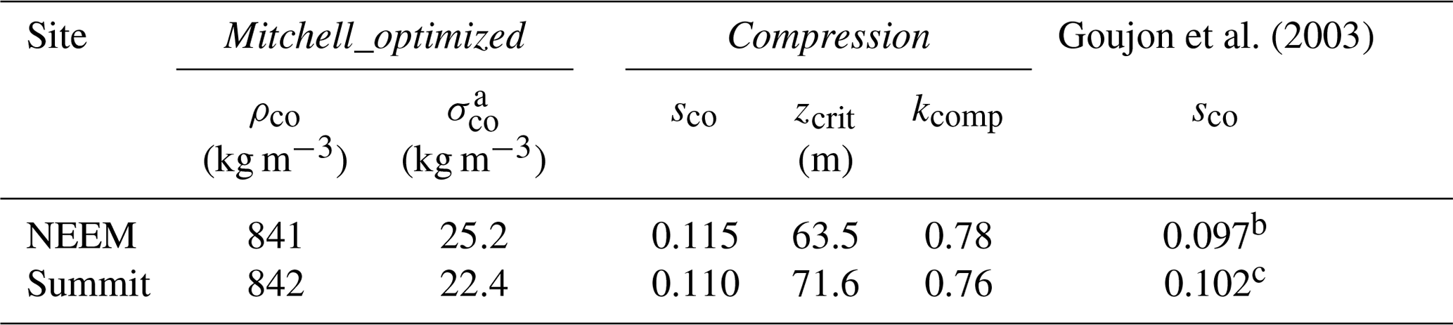
^a σ_co combines the uncertainty associated with both layering and close-off density in Mitchell et al. (2015), Eq. (6) as the two parameters cannot be optimized independently. ^b From Buizert et al. (2012). ^c Calculated from site temperature using the formulation of Martinerie et al. (1994).

At equilibrium, modeled enrichment of Ne and H₂ is controlled primarily by the ratio of the volume-weighted average pressure in the open and closed pores to the ambient pressure, adjusted for mixing. We define a new parameter (R) to describe this ratio:

$$\begin{array}{}\text{(8)}& R=\left(P_{\mathrm{bubble}}{s}_{\mathrm{c}}/s_{\mathrm{total}}+P_{\mathrm{ambient}}{s}_{\mathrm{o}}/s_{\mathrm{total}}\right)/P_{\mathrm{ambient}}.\end{array}$$

When previously published parameterizations of partitioning between open and closed pores are implemented in the model, R begins to increase too deep in the firn to capture the shallower δ²²Ne $/$ N₂ measurements (Figs. 1 an 2). To improve the simulation of the observed Ne enrichment, we introduce a new model configuration, referred to as Mitchell_optimized. In this configuration, partitioning between closed and open porosity is based on Mitchell et al. (2015, their Eq. 6). The formulation requires two site-specific parameters: (1) ρ_co, the density of the firn at complete close-off, and (2) σ_co, the uncertainty due to fine-scale variability in firn density and variability in close-off density. These two parameters are optimized to minimize the model–measurement bias for Ne enrichment at each site (Table 3; Fig. 2a and c).

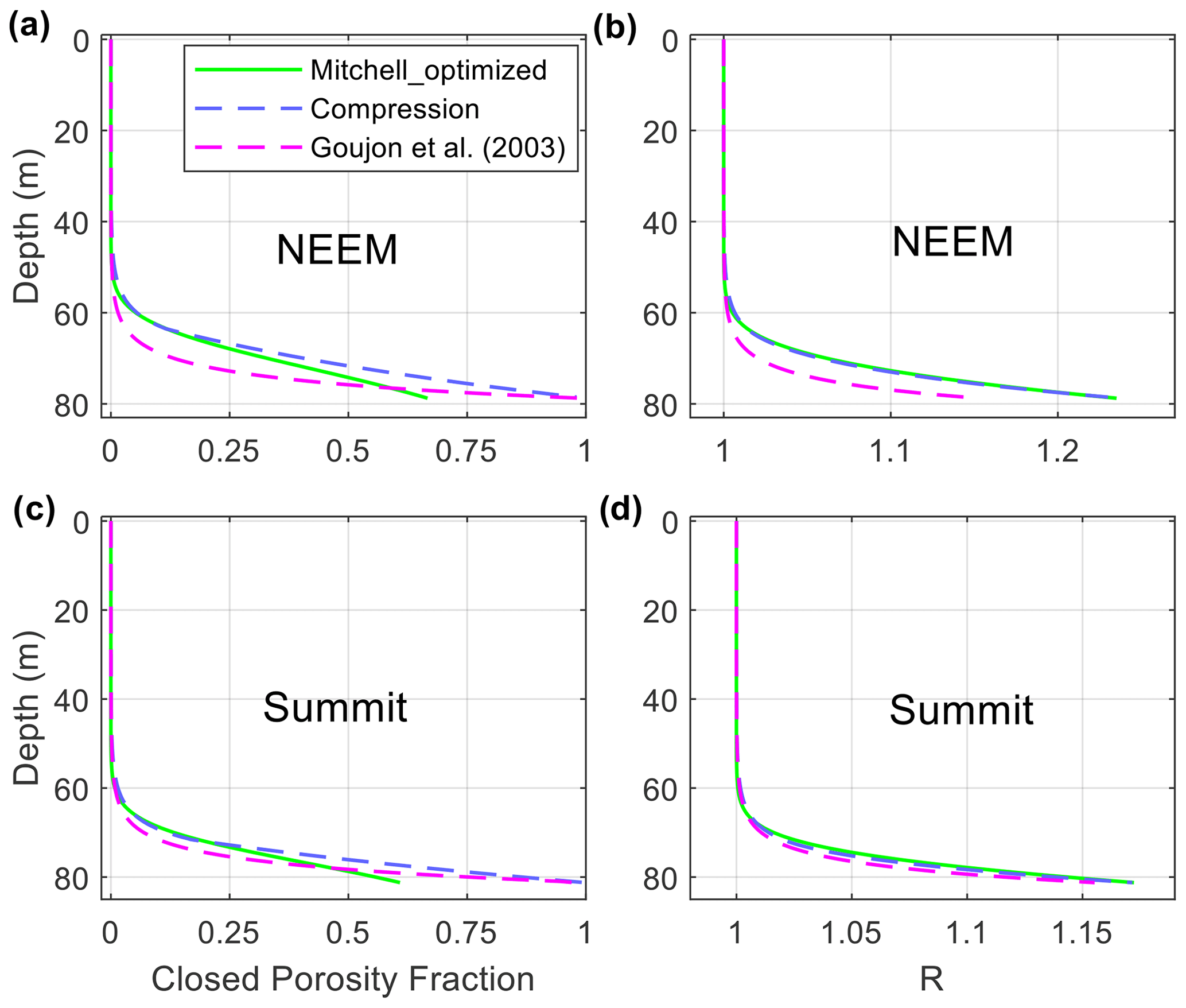
Figure 2 Closed porosity fraction ($s_{\mathrm{c}}/s_{\mathrm{total}}$) and R for NEEM (a, b) and Summit (c, d). Several model configurations with different porosity partitioning parameterizations are plotted: Mitchell_optimized (green lines), Compression (dashed purple lines), and Goujon et al. (2003; dashed magenta lines). See text for a description of each parameterization.

The Mitchell_optimized parameters are significantly different from the recommendations of Mitchell et al. (2015). Furthermore, the resulting closed porosity profiles are qualitatively different from other measured and modeled closed porosity profiles and are probably not physically realistic (Fig. 2). Bubble close-off takes place over a much broader depth range in the Mitchell_optimized configuration, and complete close-off (i.e., s_c>0.999 s_total) does not occur until depths of 111.0 m (NEEM) and 112.5 m (Summit). Firn air could only be sampled to a depth of 75.9 m (NEEM) and 80.1 m (Summit), suggesting that complete close-off is actually significantly shallower than in the Mitchell_optimized configuration.

We also examined one additional model configuration, referred to as the Compression configuration, in which we force the closed porosity profile to have a more typical complete close-off depth. In this configuration, the closed porosity above some optimized critical depth (z_crit) is parameterized as in Goujon et al. (2003; their Eq. 9) with an optimized s_co parameter. Below the critical depth, closed porosity increases linearly with depth, reaching complete close-off at the same depth as in the Goujon et al. (2003) base-case (79.2 m at NEEM and 81.5 m at Summit). A similar two-stage closed porosity parameterization was used in Severinghaus and Battle (2006). The resulting closed porosity profiles are more similar to previously published profiles and probably more realistic (Fig. 2). However, even with an optimized z_crit and s_co, we found that R increases too rapidly with depth to capture the δ²²Ne $/$ N₂ at both the top and the bottom of the lock-in zone. Therefore, to generate the necessary R profile while maintaining a realistic closed porosity profile, some other physical process must be modified in the model in addition to the closed porosity profile. Possible candidates include the rate of pressurization of bubbles, the rate of densification, and the rate of bubble close-off. A detailed observation-based investigation of these processes at these sites would require field data that do not currently exist. Here, we use the rate of bubble pressurization as an additional tuning lever to examine the sensitivity of the model results to the specific physical parameterizations in the model.

The bubble pressurization scheme used in the UCI_2 model assumes that closed bubbles compress at the same rate as the total porosity after Severinghaus and Battle (2006). Bubble trapping models that assume such iso-compression have been shown to overestimate total air content in bubbles at the Lock-in and Vostok sites in East Antarctica (Fourteau et al., 2019). In that work, better model–measurement agreement was achieved by reducing the compressibility of closed bubbles by 50 %. To reduce the compressibility of closed bubbles in our Compression model configuration, we modified the calculation of the incremental new volume of air at ambient pressure (ΔV_b(i)) occluded in bubbles between layer (i−1) and layer (i) per unit volume of firn:

$$\begin{array}{}\text{(9)}& \begin{array}{rl}& \mathrm{\Delta }{V}_{\mathrm{b}\left(i\right)}=\\ & {\displaystyle \frac{\mathrm{2}\left\{s_{\mathrm{c}\left(i\right)}-s_{\mathrm{c}(i-\mathrm{1})}\left[\left(\mathrm{1}-k_{\mathrm{comp}}\right)+k_{\mathrm{comp}}\frac{s_{\mathrm{total}\left(i\right)}}{s_{\mathrm{total}(i-\mathrm{1})}}+\frac{{\mathit{\rho }}_{\mathrm{firn}\left(\mathrm{i}\right)}}{{\mathit{\rho }}_{\mathrm{firn}(i-\mathrm{1})}}-\mathrm{1}\right]\right\}}{\left(\mathrm{1}-k_{\mathrm{comp}}\right)+k_{\mathrm{comp}}\frac{s_{\mathrm{total}\left(i\right)}}{s_{\mathrm{total}(i-\mathrm{1})}}+\mathrm{1}}},\end{array}\end{array}$$

where k_comp is a dimensionless free parameter that represents the degree of compressibility of the bubbles. In the limit of k_comp=1, Eq. (9) reduces to Eq. (A12) of Severinghaus and Battle (2006), and bubbles compress at the same rate as the open pores. In the limit of k_comp=0, the bubbles are completely incompressible. In the Compression configuration, k_comp is simultaneously optimized with z_crit and s_co to achieve agreement between modeled and measured Ne enrichment (Figs. 1 and 2; Table 3).

Both alternative model configurations (Mitchell_optimized and Compression) yield a greatly improved fit between modeled and measured Ne enrichment at NEEM and Summit. The alternative model configurations are considered empirical tuning methods to fit the Ne data and should not be used to draw conclusions about the underlying firn physics. Further investigation of bubble pressurization, firn layering, and bubble close-off using high-resolution measurements of density, porosity, and air content, in conjunction with measurements of highly diffusive trace gases like Ne or He, would be useful in constraining the underlying physics of pore close-off fractionation for future Greenland firn air work.

The Mitchell_optimized and Compression configurations yield very similar reconstructions. As long as accurate Ne enrichment is achieved, the reconstructions are insensitive to the specific parameterization of closed porosity (Sect. 4; Figs. 3 and 5). This result is important given the uncertainty and ad hoc nature of our model tuning. For the sake of simplicity, we use the Mitchell_optimized configuration as the default model for NEEM and Summit for the remainder of this work. Comparisons between the Mitchell_optimized and Compression configurations are shown in Figs. 3 and 5. Additionally, we note that the choice of configuration has a negligible effect on the model result for the tuning gases (Fig. S5 for CO₂ and CH₄).

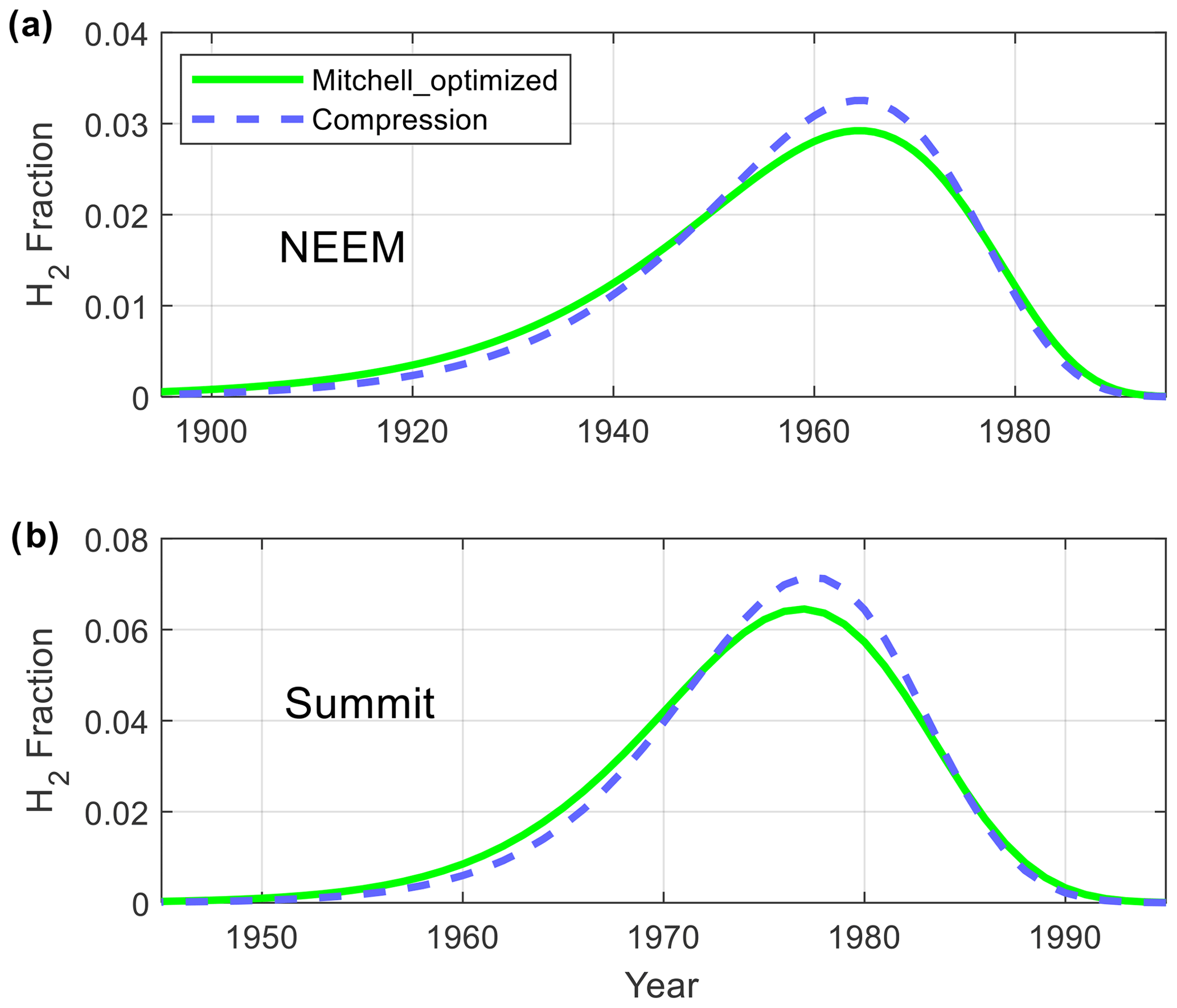
Figure 3 Calculated H₂ age distributions (Green's functions) for depths of 75.9 m at NEEM (a) and 80.1 m at Summit (b) using two different parameterizations for the partitioning of closed and open porosity with depth. The Mitchell_optimized (green lines) and Compression (dashed purple lines) configurations produce very similar age distributions.

3.3 Inversion methods

The firn air measurements are inverted to recover an atmospheric history of H₂ from each site. The inversion technique employs depth-dependent age distributions or “Green's functions” (G; Fig. 3; Rommelaere et al., 1997). The firn air model is initialized with no H₂ in the firn air column, then forced with a transient 1-year unit pulse of H₂ at the surface. The model is integrated for 300 years, and the evolution of the pulse is tracked as a function of depth and time to produce the Green's functions. The age distributions grow older and broader with depth (Fig. S1 in the Supplement). For most gases, the Green's functions integrate to 1 at every depth. In the case of H₂ and Ne, the sum of the Green's functions in the lock-in zone is slightly greater than 1 due to pore close-off fractionation. Given an atmospheric history (H_2(atm)), modeled levels of H₂ in the firn (H_2(firn)) are calculated according to Eq. (10):

$$\begin{array}{}\text{(10)}& {\mathrm{H}}_{\mathrm{2}\left(\mathrm{firn}\right)}\left(z\right)=\sum _{t=\mathrm{0}}^{\mathrm{300}}{\mathrm{H}}_{\mathrm{2}\left(\mathrm{atm}\right)}\left(t\right)\cdot G(z,t).\end{array}$$

Using Green's function allows for rapid iteration over many possible atmospheric histories without running the firn air model in forward mode. The inversion problem is under-constrained. Multiple atmospheric histories can provide good agreement with the measured depth profile, and additional constraints are required to yield a unique solution. In previous studies, the additional constraint has been implemented as a smoothing parameter (Patterson et al., 2020, 2021; Petrenko et al., 2013; Rommelaere et al., 1997). In this work, we rely instead on the assumption of autocorrelation and utilize the probabilistic modeling software package, Stan (mcstan.org). Stan was previously used for firn air reconstructions by Aydin et al. (2020). As in that work, we use Stan to implement a Bayesian hierarchical model in which the atmospheric history is treated as an autocorrelated random variable:

$$\begin{array}{}\text{(11)}& {\mathit{m}}_{\mathrm{atm}}\left[t_i\right]\sim N\left({\mathit{m}}_{\mathrm{atm}}\left[t_{i-\mathrm{1}}\right],\mathit{\alpha }{\mathit{m}}_{\mathrm{atm}}\left[t_{i-\mathrm{1}}\right]\right),\end{array}$$

where N is the normal distribution, and m_atm is a vector of length i that contains the discrete atmospheric H₂ dry-air mole fraction history with a time step of 1 year. The atmospheric mixing ratio at time t_i is normally distributed around the atmospheric mixing ratio at time t_i−1 with a standard deviation of αm_atm[t_i−1]. α is a positive scalar and is varied as a free parameter. The atmospheric history is related to the firn air measurements:

$$\begin{array}{}\text{(12)}& {\mathit{h}}_{\mathrm{obs}}\sim N\left(\mathbf{G}{\mathit{m}}_{\mathrm{atm}},\mathit{\sigma }\right),\end{array}$$

where h_obs is a vector of length n, which contains the measured H₂ levels at each depth, G is an n by i matrix where each row corresponds to the Green's function for that unique depth (referred to as the “kernels” by Rommelaere et al., 1997), and σ is a vector of length n, which contains the analytical uncertainties of the firn air measurements. Stan samples the joint posterior probability distribution for the parameters m_atm and α using a fast Hamiltonian Markov chain Monte Carlo algorithm (Carpenter et al., 2017). Parameters are sampled from uniform prior distributions unless otherwise specified. Inversions are carried out using the MATLAB–Stan 2.15.1.0 interface to cmdstan 2.27.0. The advantages of this method over other methods include (1) no arbitrarily specified smoothing criteria being imposed (instead the atmospheric history is assumed to be autocorrelated) and (2) Stan allowing us to easily explore sensitivity to assumptions about the data by encoding those assumptions as priors.

In Greenland, H₂ levels in the upper firn layers are strongly influenced by seasonal variations, and firn air reconstructions cannot accurately reconstruct such high-frequency variability. Therefore, measurements from the upper part of the firn were excluded from the reconstructions. A cut-off depth was determined by forcing the firn air model in forward mode with an atmospheric history that consists of constant annually averaged H₂ levels with a realistic seasonal cycle imposed. Depths where the H₂ concentration varied by more than 1 % from the annual average were excluded from the reconstruction. The cut-off depths were 62 and 66 m for NEEM and Summit. Unlike Greenland, Antarctic H₂ reconstructions are not sensitive to seasonality, primarily because seasonal variability in atmospheric H₂ levels over Antarctica is less than half that of seasonal variability over Greenland.

4 Atmospheric reconstructions

Atmospheric H₂ reconstructions were carried out for each Greenland site independently (Fig. 4). The NEEM and Summit sites have different physical characteristics (mean annual temperature and accumulation rate) and were sampled at different times, yielding different firn air age distributions (Fig. 3). The model inversions yield generally good agreement between the modeled and measured depth profiles for NEEM (Fig. 4b). Agreement is also good at Summit, except at the bottom of lock-in where the modeled depth profile increases monotonically with depth while the deepest measurement shows a slight decrease. The disagreement in trend at the bottom of the firn is due to a single firn air measurement that insufficiently constrains H₂ levels prior to 1975. A decreasing trend in the modeled depth profile is obtained by halving the uncertainty in the Summit firn measurements (Fig. S2). This more tightly constrained reconstruction yields H₂ levels 15–20 ppb lower than the base-case Summit reconstruction prior to 1975 (Fig. 4a). For the post-1975 time period during which we consider the reconstruction valid, the differences between the two reconstructions are negligible.

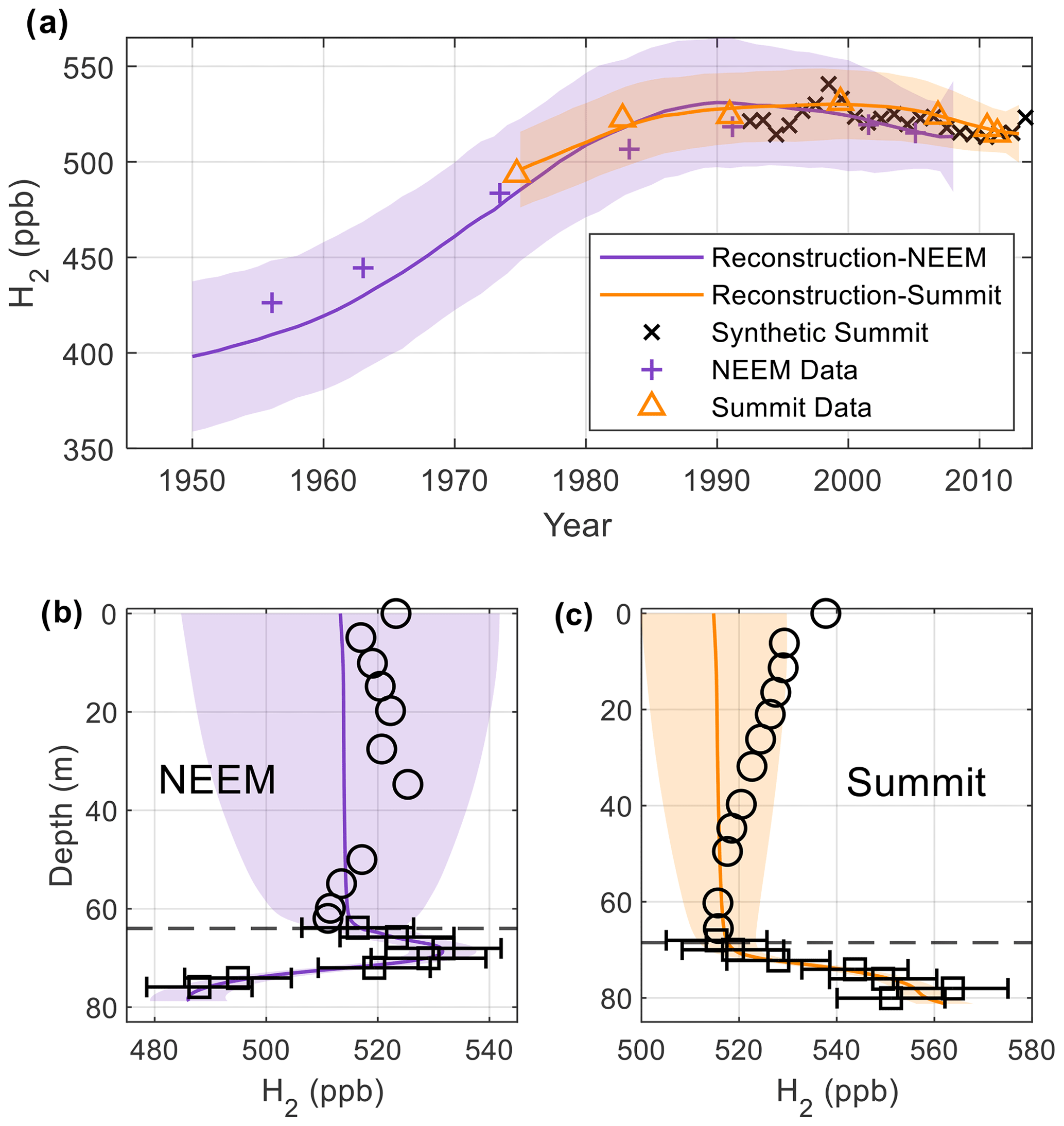
Figure 4 H₂ atmospheric histories and firn air profiles reconstructed independently from firn air measurements at Greenland sites NEEM and Summit using the Mitchell_optimized model configuration. (a) NEEM (purple)and Summit (orange), with ±1σ uncertainty (shaded regions). Firn air measurements adjusted for pore close-off fractionation are plotted against mean age (crosses and triangles). Black x marks are the synthetic Summit history from Pétron et al. (2023) and Langenfelds et al. (2002; Sect. 5). (b, c) Measured and modeled depth profiles at NEEM and Summit, respectively. Squares with error bars are measurements used in the reconstruction, and circles are measurements excluded due to seasonality. Colored lines and shading are the depth profiles modeled from the histories in (a) with the propagated ±1σ uncertainty. The dashed black lines indicate the top of the lock-in zone.

Firn air measurements from NEEM constrain atmospheric H₂ levels after 1950. The NEEM reconstruction shows atmospheric H₂ increasing from 1950–1990 at an average rate of 3.3 ppb yr⁻¹ (400–530 ppb). After 1990, atmospheric levels decrease slowly at an average rate of 0.8 ppb yr⁻¹, reaching 515 ppb in 2008. Summit firn air is younger, yielding an atmospheric history beginning in 1975. The Summit reconstruction shows atmospheric H₂ increasing from 500–528 ppb from 1975 to 1990, an average rate of 1.1 ppb yr⁻¹. After 1994 atmospheric H₂ levels are mostly stable until 2003. After 2003, atmospheric H₂ decreases slowly at a rate of 1.3 ppb yr⁻¹, reaching 515 ppb in 2013.

A “joint” reconstruction was carried out in which the most probable atmospheric history given the firn air data from both Greenland sites is calculated (Fig. 5). Reconstructed atmospheric H₂ levels increase from 390 ppb in 1950 to 530 ppb in 1987 at an average rate of 3.8 ppb yr⁻¹. After 1987, atmospheric H₂ levels are stable near 530 ppb until 2002, when they begin to decrease slowly, reaching 515 ppb in 2013. There is good agreement between the modeled and measured depth profiles for the joint reconstruction, and the differences between the Mitchell_optimized configuration and Compression configuration are negligible (Fig. 5).

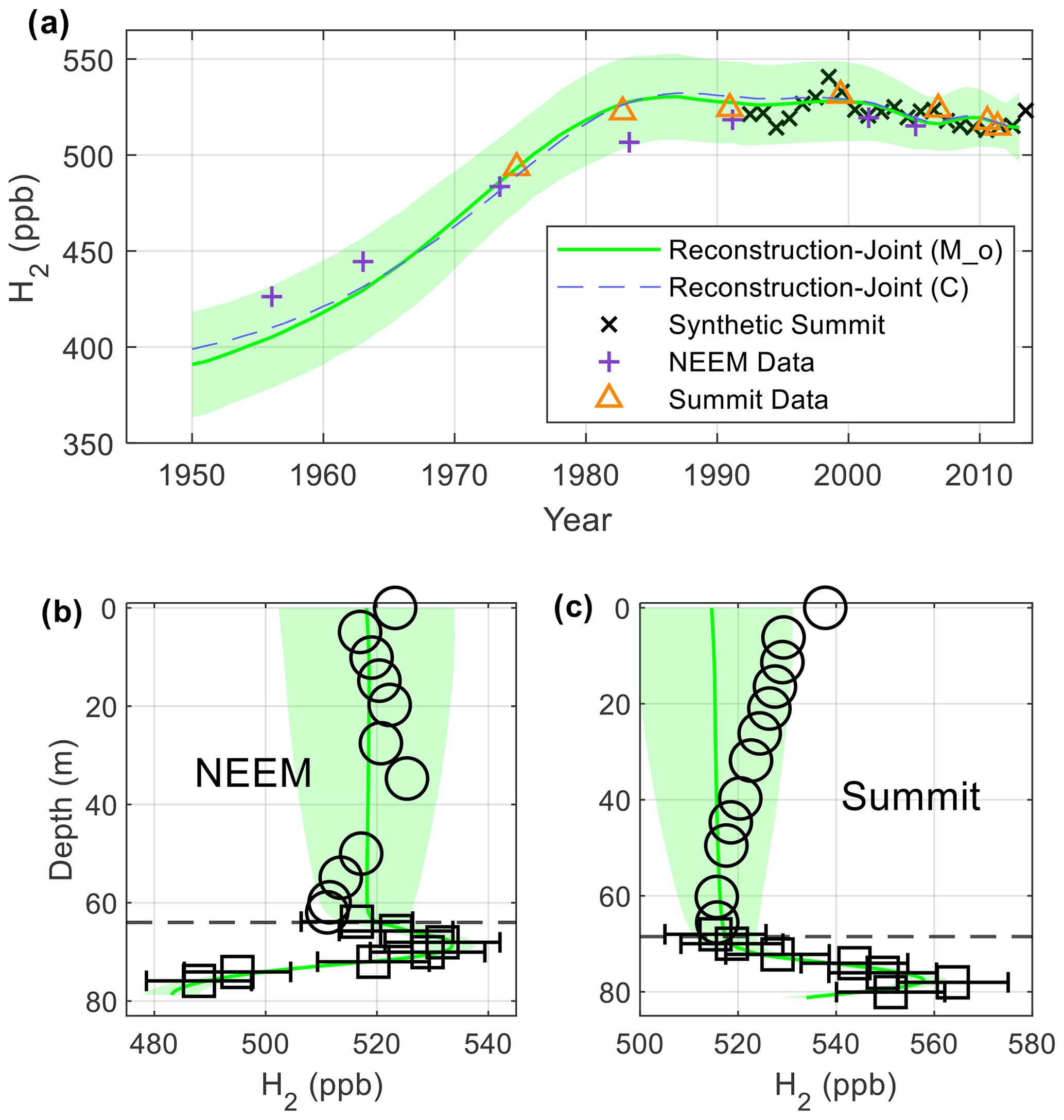
Figure 5 Joint reconstructions using firn air profiles at Greenland sites NEEM and Summit. (a) Joint reconstruction (green line and ±1σ uncertainty shading) using the Mitchell_optimized model configuration; dashed purple line – reconstruction result using the Compression configuration. Other markers are as in Fig. 4a. (b, c) Modeled depth profiles at NEEM and Summit with symbols as in Fig. 4.

A joint reconstruction was also carried out for the two Antarctic sites (Fig. 6). Because of unique site characteristics, the firn air at Megadunes is old, and the Antarctic H₂ levels may be reconstructed beginning in 1875 (Severinghaus et al., 2010). The reconstruction shows H₂ levels stable near 330 ppb from 1875–1900. After 1900, atmospheric H₂ levels increase at an average rate of 1.6 ppb yr⁻¹, reaching 440 ppb in 1970. After 1970, atmospheric H₂ levels increase more rapidly at a rate of 4.11 ppb yr⁻¹, reaching 550 ppb in 1997 and stabilizing thereafter. There is good agreement between the modeled and measured depth profiles at the Antarctic sites. The South Pole data suggest some additional fluctuations in the growth rate of atmospheric H₂ during the 20th century, particularly a reduced growth rate from 1940–1955 (Fig. 6). These fluctuations are not present in the joint reconstruction due to the smoothing inherent in the inversion method. This is an inherent limitation of firn air reconstructions.

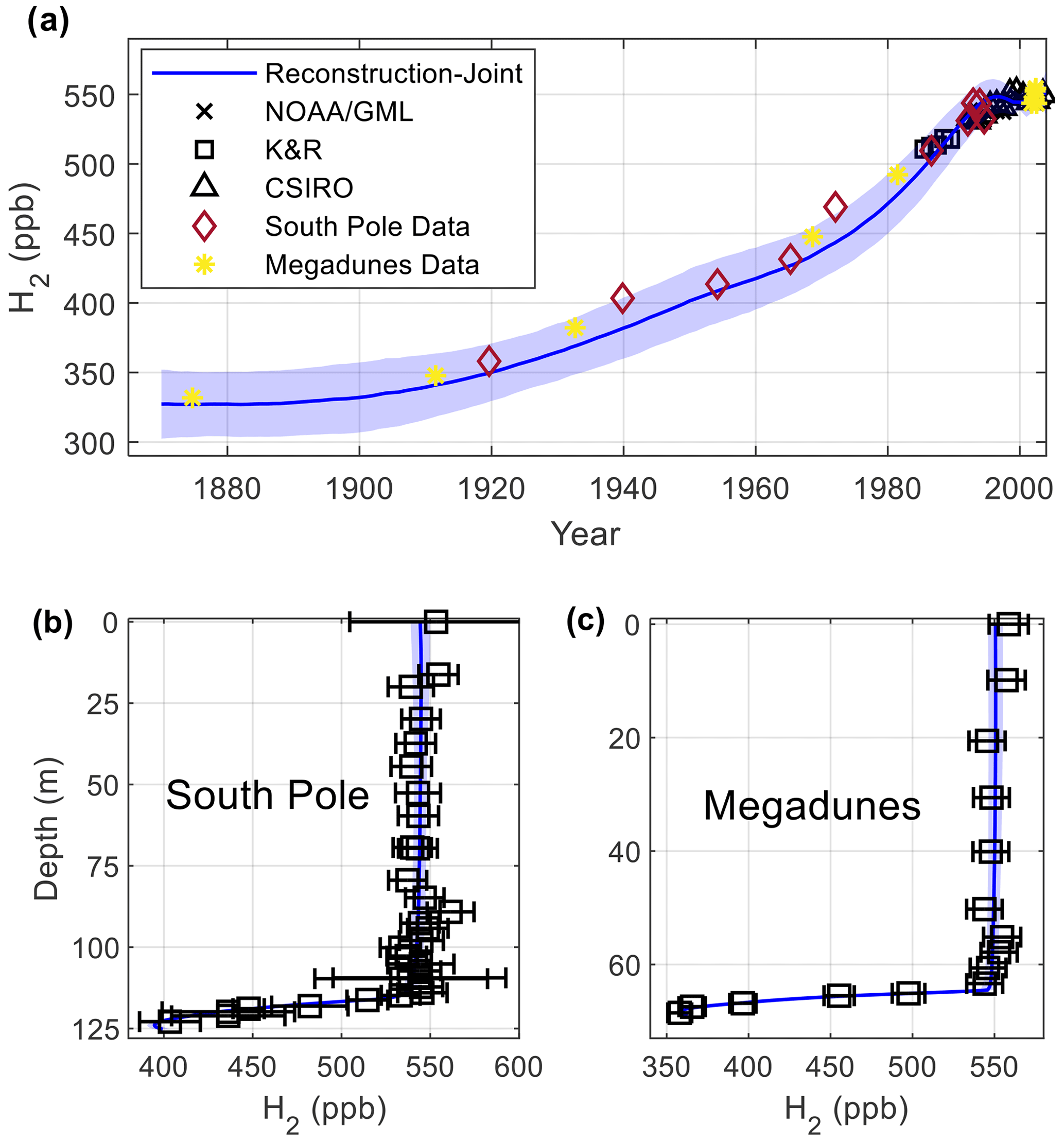
Figure 6 Joint reconstruction using firn air profiles at the two Antarctic sites. (a) Blue line and shading – reconstruction result and associated ±1σ uncertainty; black x marks – H₂ annual means from measurements made by NOAA/GML at Palmer, Syowa, South Pole, and Halley stations (Antarctica), as well as Cape Grim Observatory (Tasmania) (Novelli et al., 1999; Novelli, 2006); black circles – H₂ annual means from measurements made by CSIRO at Casey, South Pole, and Mawson stations, (Antarctica), as well as Cape Grim and Macquarie Island (Tasmania) (Langenfelds et al., 2002). H₂ annual means are from measurements made by Khalil and Rasmussen (1990) at Palmer Station, Antarctica, and Cape Grim, Tasmania. Red diamonds and yellow stars – 10 deepest firn air measurements plotted against modeled mean age for South Pole and Megadunes, respectively; the data have been adjusted for pore close-off fractionation. (b) Black markers – measured H₂ depth profile at South Pole; blue line and shading – modeled depth profile using the atmospheric history plotted in blue in (a) with the propagated ±1σ uncertainty. The dashed black line indicates the top of the lock-in zone. Panel (c) is as in (b) for Megadunes.

5 Comparison of firn air reconstructions with atmospheric flask measurements and previously published reconstructions

Petrenko et al. (2013) produced two atmospheric H₂ reconstructions from the NEEM firn air data. The reconstructions were generated using two different models: LGGE-GISPA and INSTAAR. Neither of those models includes pore close-off fractionation, and Patterson et al. (2021) suggested that the maximum in atmospheric H₂ inferred from the NEEM firn air could be an artifact of ignoring pore close-off fractionation. Petrenko et al. (2013) used the matrix inversion method of Rommelaere et al. (1997), which requires a prescribed smoothing parameter to fully constrain the inversion. Those results were corrected for a calibration revision (see the Supplement) and are compared to our joint reconstruction (Fig. 8a). The LGGE-GISPA reconstruction shows a rapid rise in H₂ levels from 1960-1990 and a rapid decrease from 1990–2008. The INSTAAR reconstruction shows H₂ levels rising more gradually from 1960–1985 and decreasing gradually thereafter. The rate of increase in H₂ levels between 1960 and 1980 in our joint reconstruction is very similar to the rates of increase in the LGGE-GISPA reconstruction. However, in our joint reconstruction, the rate of increase slows after 1980, and H₂ levels plateau by 1990. Here, we compare our reconstruction to available atmospheric H₂ flask measurements from the high northern latitudes in order to assess the validity of our reconstructed plateau during the 1990s (Fig. 7).

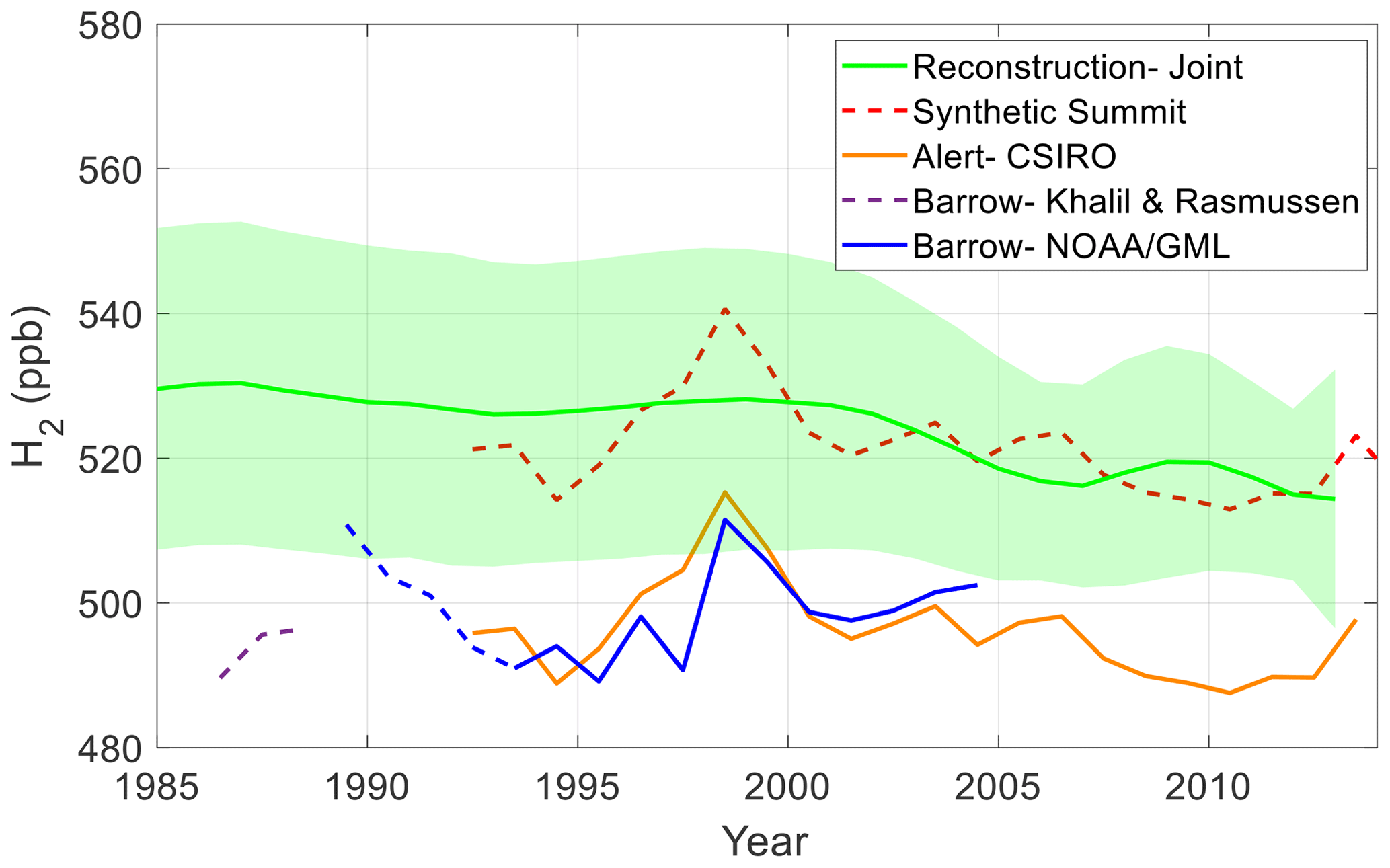
Figure 7 Comparison of the joint Greenland firn air reconstruction with high-northern-latitude flask measurements. Green line and shading – joint reconstruction as in Fig. 5a; dashed red line – annual mean synthetic Summit H₂ history (Sect. 5; Pétron et al., 2023; Langenfelds et al., 2002); yellow line – annually averaged flask measurements from Alert, Nunavut, made by CSIRO (Langenfelds et al., 2002); dashed purple line – annually averaged flask measurements from Barrow (now Utqiaġvik), Alaska, made by Khalil and Rasmussen (1990); blue line – annually averaged flask measurement from Barrow, Alaska, made by NOAA/GML (Novelli et al., 1999; Novelli, 2006). Measurements from NOAA/GML were empirically corrected to the MPI09 calibration scale using a matched flask intercomparison project between CSIRO and NOAA/GML. Note: measurements from Khalil and Rasmussen (1990) and NOAA/GML before 1993 are subject to additional calibration uncertainty as discussed in the text.

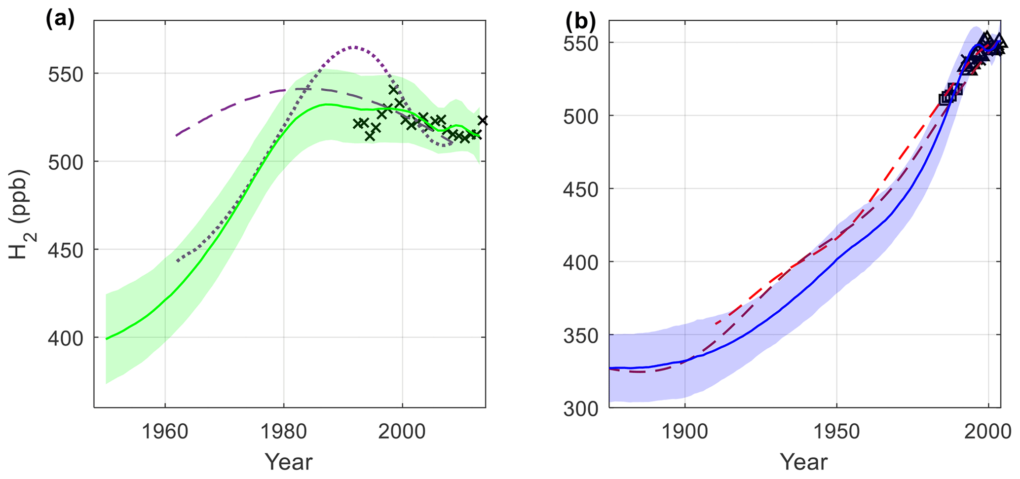
Figure 8 Comparison of our joint reconstructions with previously published firn air reconstructions. (a) Green line and shading – joint Greenland reconstruction as in Fig. 5a; purple lines – reconstructions from Petrenko et al. (2013) using the LGGE-GISPA model (dotted line) and INSTAAR model (dashed line); black x marks – annual mean synthetic Summit H₂ history (Sect. 5; Pétron et al., 2023; Langenfelds et al., 2002). (b) Blue line and shading – joint reconstruction as in Fig. 6a; dashed maroon line – South Pole firn air reconstruction from Patterson et al. (2020); dashed red line – Megadunes firn air reconstruction from Patterson et al. (2021); black x marks – H₂ annual means from measurements made by NOAA/GML at Palmer, Syowa, South Pole, and Halley stations (Antarctica), as well as Cape Grim Observatory (Tasmania) (Novelli et al., 1999; Novelli, 2006); black circles – H₂ annual means from measurements made by CSIRO at Casey, South Pole, and Mawson stations (Antarctica), as well as Cape Grim and Macquarie Island (Tasmania) (Langenfelds et al., 2002); H₂ annual means from measurements made by Khalil and Rasmussen (1990) at Palmer Station, Antarctica, and Cape Grim, Tasmania.

Direct comparisons between the firn reconstructions and atmospheric measurements at other sites are complicated by spatial variability in H₂ levels in the high northern latitudes. The best temporal coverage for flask air H₂ measurements is from the Barrow (Alaska – now Utqiaġvik) and Alert (Nunavut) sampling sites. Both sites sample the boundary layer and are influenced by their proximity to seasonally active soils. H₂ levels over Greenland are more representative of the free troposphere due to higher elevation and remoteness from active soils. To make this comparison, we utilize NOAA/GML measurements at Alert (Nunavut) and Summit (Greenland) from 2010–present (revised to the MPI09 calibration scale; Pétron et al., 2023) and CSIRO measurements from Alert from 1992 onwards (also on the MPI09 scale).

During the 12 years of NOAA/GML measurements at Summit and Alert, the offset between Summit and Alert varies from a minimum of 18.9 ppb to a maximum of 29.4 ppb; the mean offset is 25.4 ppb ± 3.0 ppb (1σ), with Summit levels higher than Alert. We added this offset to the longer CSIRO Alert time series to generate a longer “synthetic Summit” flask history, assuming that the offset remains constant through time (Figs. 4–5 and 7–8). The most conspicuous feature of the synthetic Summit history is a sharp peak in H₂ levels during 1998 which can be attributed to increased biomass burning emissions during the strong 1997–1998 El Niño event (Langenfelds et al., 2002; van der Werf et al., 2004). Firn air cannot resolve such high-frequency variability due to diffusive smoothing, so that feature is absent from our reconstructions. Excepting the 1998 peak, synthetic Summit H₂ levels are largely constant between 525 and 515 from 1992–2013, in good agreement with our reconstructed 1990s plateau.

We also examined the atmospheric data for evidence of the H₂ maximum around 1990 indicated by the firn air reconstructions of Petrenko et al. (2013). If this peak had occurred in the atmosphere, we would expect similar trends at all of the high-latitude flask sites despite the differences in absolute H₂ levels. Here we examine flask measurements from Barrow, Alaska (Khalil and Rasmussen, 1990; NOAA/GML), and Alert, Canada (CSIRO; Fig. 7). The measurements from NOAA/GML from 1992–2005 were corrected to the MPI09 calibration scale using the matched flask intercomparison project mentioned previously (Sect. 2.2). The Khalil and Rasmussen (1990) data are reported on an independent calibration scale which has not been intercompared to the MPI09 calibration scale. The Barrow data from Khalil and Rasmussen (1990) show an increase in atmospheric H₂ of 2.1 ppb yr⁻¹ from 1985–1988 and the subsequent NOAA/GML data show a decrease in atmospheric H₂ from 1989–1993 at a rate of 5.0 ppb yr⁻¹. The reason for the rapid decrease in observed H₂ levels in the NOAA/GML data is not clear. At that time, anthropogenic emissions of H₂ were likely decreasing but not rapidly enough to account for the observed decrease (Hoesly et al., 2018; Paulot et al., 2021). It is possible that the observed decrease is linked to NOAA's drifting calibration scale as discussed in Sect. 2.2. Together, the trends in these two data sets imply a maximum in atmospheric H₂ in 1989. However, the strength of this conclusion is questionable because the flask intercomparison project did not include data prior to 1992. Furthermore, the NOAA/GML Barrow data are subject to additional uncertainty due to the single-point calibration of those measurements and the nonlinearity of the HgO-RGA detector used by NOAA/GML at the time. Further paleo-studies are warranted to investigate the brief but dramatic decrease in the Barrow data from 1989–1993. From 1993–2010, there is no discernible trend in atmospheric H₂ at either Barrow or Alert. Generally, the H₂ plateau from our joint reconstruction is more consistent with 1990s flask data than the sustained and dramatic decrease in the Petrenko et al. (2013) reconstructions.

Firn diffusion imposes smoothing on atmospheric histories and prevents the reconstruction of high-frequency atmospheric variability. To test whether a brief, sharp decline in atmospheric H₂ prior to a plateau, as suggested by the flask measurements, is compatible with the firn air measurements, we forced the firn air model with a synthetic atmospheric history. The synthetic history was identical to the joint reconstruction before 1980. After 1980, H₂ levels in the synthetic history increase linearly to 546 ppb in 1989. There is a 5 ppb yr⁻¹ decrease from 1989–1993 (as observed in the Barrow flask measurements) and subsequently H₂ levels are the same in the synthetic history as in the joint reconstruction. The depth profiles generated by the model when forced with the synthetic history show reasonable agreement with the measured firn H₂ (Fig. S4). Therefore, a short, rapid decline in atmospheric H₂ levels around 1990 cannot be excluded as a possibility.

The results of the joint Antarctic reconstruction are compared to previously published reconstructions from those individual sites from (Patterson et al., 2020, 2021; Fig. 8b). The differences between the joint reconstructions and the previously published reconstructions are relatively minor. The joint reconstruction shows a slower increase in H₂ levels prior to 1970 and a more rapid increase from 1970–1997, while the reconstructions of Patterson et al. (2020, 2021) show a more uniform rate of increase during the 20th century. This is likely due to the use of an arbitrary smoothing parameter in the earlier studies, while an autocorrelation function was used in the joint reconstruction. Additionally, there are small differences in the tuning of the firn air model compared to the earlier publications. The joint Antarctic reconstruction is in good agreement with available flask measurements from high southern latitudes, which show H₂ levels rising throughout the 1990s and plateauing thereafter (Fig. 8b).

6 In situ production

Previous research has found evidence of in situ production of CO in the Arctic snowpack. It is important to consider the possibility of in situ H₂ production at the Greenland sites because H₂ and CO are co-produced by the photooxidation of carbonyl-containing precursors. CO has been shown to be produced photochemically from CH₂O in surface snow (Haan et al., 2001). At Devon Island, Canada, CO levels in the firn increased steadily with depth in both the diffusive and lock-in zones, exhibiting clear evidence of in situ production (Clark et al., 2007). By contrast, NEEM and Summit firn air measurements both exhibit CO maxima in the firn air column associated with a late 20th century atmospheric maximum, with CO levels decreasing with increasing depth (Petrenko et al., 2013). Petrenko et al. (2013) concluded in situ production at those sites was not sufficient to bias the atmospheric reconstruction. Those researchers used three lines of evidence to support their conclusion. First, the ice age at the depth of the observed lock-in zone CO peak is different at the two sites, so the peak cannot be attributed to a widely deposited layer of organic impurities. Second, the $\mathrm{CO}/{\mathrm{CH}}_{\mathrm{4}}$ ratio at a given depth is in reasonable agreement at NEEM and Summit. CO and CH₄ have similar gas-phase diffusivities, so the mean age of the two gases at a given depth is comparable. CH₄ is known to be well preserved in Greenland firn air. If in situ production differentially affected CO levels at the two sites, it would be expected that $\mathrm{CO}/{\mathrm{CH}}_{\mathrm{4}}$ ratios would diverge. Third, forcing a firn air model with an atmospheric-flask-derived CO history yields good agreement with the measured depth profile down to the top of lock-in zone where the firn air is too old to be constrained by flask measurements.

Greenland ice cores do exhibit evidence of in situ CO production. Early discrete measurements on Eurocore ice showed low, steady pre-industrial CO levels (Haan and Raynaud, 1998; Haan et al., 1996). By contrast, Faïn et al. (2022) reported higher and more variable CO levels from several Greenland sites (including NEEM) using continuous-flow and discrete methods. The elevated CO levels were apparently associated with localized organic impurities in the ice. The high variability in CO detected by the continuous-flow method is not compatible with continuous production in the firn, where such signals should be smoothed by diffusion. It is therefore likely that the high-frequency variability observed by Faïn et al. (2022) originated below the lock-in zone. However, the ice core data do not preclude the possibility of some in situ production having occurred in the overlying firn.

The production of CO in Greenland firn air and ice is not well understood, and no physical mechanism has been proposed that can explain all of the observations. If the production is photochemical, one would expect it to be much faster in the firn than in ice due to the much larger actinic flux at the surface. Until the mechanism is established, it is difficult to assess whether and to what extent in situ production might influence firn air H₂. Depending on the depth and mechanism, production of H₂ in the firn column would cause a high bias during some or all of our atmospheric reconstructions. Further research on this issue is needed.

7 Summary and conclusions

In this study we use all available firn air measurements of H₂ at Greenland and Antarctic sites to reconstruct atmospheric H₂ levels over the past century. The joint Antarctic reconstruction covers the 1875–2003 period and is based on firn air measurements from South Pole and Megadunes (Patterson et al., 2020, 2021). That reconstruction shows good agreement with the atmospheric flask network since the late 1980s. The good fit between measured and simulated Ne enrichment obtained using the our firn air model gives us high confidence in the modeling of pore close-off fractionation at the Antarctic sites.

Reconstructing H₂ levels over Greenland is more challenging because of the additional tuning required to simulate the enrichment of Ne induced by pore close-off in the firn. To fit the Ne firn data, we used one model configuration with an optimized but unrealistic closed porosity profile (Mitchell_optimized) and one model configuration that uses a more realistic, optimized closed porosity profile in conjunction with an optimized rate of bubble pressurization (Compression). To our knowledge, the rate of bubble pressurization in Greenland firn has not been studied in detail. Both model configurations yield improved agreement between modeled and measured Ne at the Greenland firn sites with negligible effects on the model results for less permeable trace gases like CO₂ and CH₄ (Figs. 2 and S5). The results of our reconstructions are insensitive to the choice of model configuration.

The Mitchell_optimized and Compression model configurations are empirical tuning methods and do not address uncertainty around the physics underlying the observed enrichment induced by pore close-off in Greenland firn air. A path to increasing confidence in firn air reconstructions for H₂ is to obtain new observations of firn air chemistry with high-resolution measurements of firn density, porosity, and bubble total air content. In the absence of additional measurements, we believe that the results presented in Fig. 9 are the best estimate for the evolution (and uncertainty) of atmospheric H₂ during the 20th century over Antarctica and Greenland. Ice core records at high-accumulation sites should also be collected in order to constrain H₂ levels over the late pre-industrial and industrial eras. Such records will be important to better understand the global H₂ cycle, the impact of human activities on H₂ in the past, and the atmospheric response to increasing anthropogenic H₂ emissions in a warming climate.

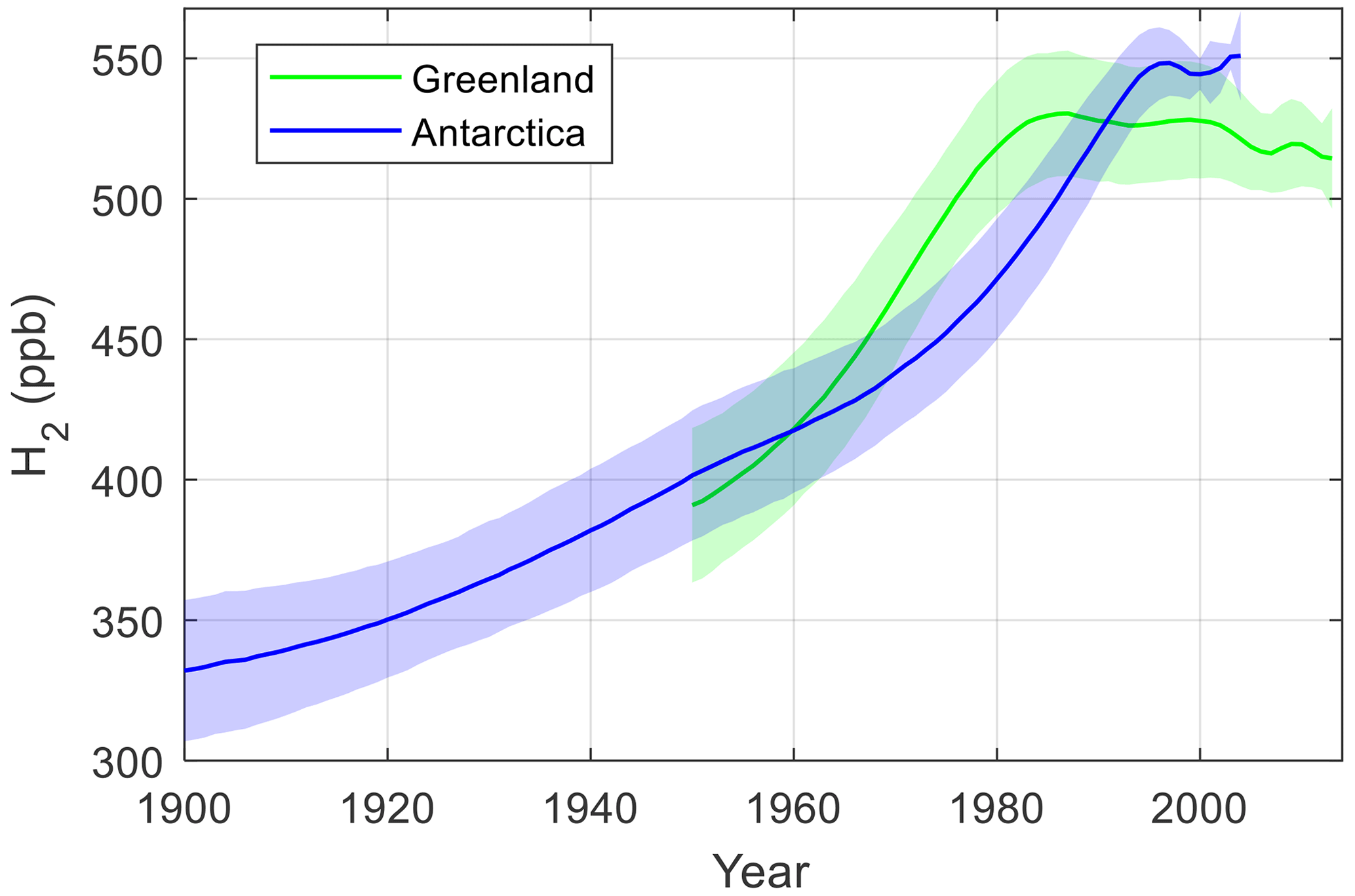
Figure 9 Best estimates for the atmospheric history of H₂ in Greenland and Antarctica over the past century. Green line – joint Greenland firn air reconstruction as in Fig. 5a. Blue line – joint Antarctic firn air reconstruction as in Fig. 6a. Shaded areas are ±1σ uncertainties.

One surprising result is that our reconstructions show higher H₂ levels over Greenland than over Antarctica prior to 1990. This implies a reversal in the sign of the interhemispheric difference during the late 20th century. It is believed that Northern Hemisphere H₂ levels are lower than Southern Hemisphere levels today due to strong uptake of atmospheric H₂ by Northern Hemisphere soils. The N–S interhemispheric difference in atmospheric H₂ occurs in spite of the fact that direct anthropogenic emissions of H₂ occur predominantly in the Northern Hemisphere. The dominance of northern hemispheric soil sink is largely a function of the asymmetry in land area between the two hemispheres. While the soil sink may vary over time due to changes in ecosystems, land use, or climate, a dramatic change would be required in order to have caused a reversal of the interhemispheric difference. In this respect, the firn air reconstructions present a challenge to our understanding of the global atmospheric H₂ budget. The reversal in the sign of the reconstructed interhemispheric is sensitive to our assumption that the in situ production does not affect H₂ in the NEEM and Summit firn, and the careful examination of this assumption is warranted.